Abstract
Convolutional neural networks (CNNs) and graph convolutional networks (GCNs) have led to promising advancements in hyperspectral image (HSI) classification; however, traditional CNNs with fixed square convolution kernels are insufficiently flexible to handle irregular structures. Similarly, GCNs that employ superpixel nodes instead of pixel nodes may overlook pixel-level features; both networks tend to extract features locally and cause loss of multilayer contextual semantic information during feature extraction due to the fixed kernel. To leverage the strengths of CNNs and GCNs, we propose a multiscale pixel-level and superpixel-level (MPAS)-based HSI classification method. The network consists of two sub-networks for extracting multi-level information of HSIs: a multi-scale hybrid spectral–spatial attention convolution branch (HSSAC) and a parallel multi-hop graph convolution branch (MGCN). HSSAC comprehensively captures pixel-level features with different kernel sizes through parallel multi-scale convolution and cross-path fusion to reduce the semantic information loss caused by fixed convolution kernels during feature extraction and learns adjustable weights from the adaptive spectral–spatial attention module (SSAM) to capture pixel-level feature correlations with less computation. MGCN can systematically aggregate multi-hop contextual information to better model HSIs’ spatial background structure using the relationship between parallel multi-hop graph transformation nodes. The proposed MPAS effectively captures multi-layer contextual semantic features by leveraging pixel-level and superpixel-level spectral–spatial information, which improves the performance of the HSI classification task while ensuring computational efficiency. Extensive evaluation experiments on three real-world HSI datasets demonstrate that MPAS outperforms other state-of-the-art networks, demonstrating its superior feature learning capabilities.
1. Introduction
In recent years, research has uncovered extensive applications for hyperspectral images (HSIs) in diverse fields, such as land management [1,2,3], resource exploration [4,5,6], urban rescues [7,8], military investigations [9,10] and agricultural production [11,12]. This is mainly attributed to the abundance of spatial and spectral information available in HSIs [13,14]. Due to its applicability, HSI classification has attracted considerable attention. HSI classification involves the assignment of class labels to individual image elements, representing the features within the HSI [15].
Researchers have attempted numerous times to achieve more accurate land cover classification. In the preceding decades, the field of HSI classification has witnessed the incorporation of machine learning techniques. Classical machine learning methods, such as K-nearest neighbor [16], logistic regression [17], local binary pattern (LBP) [18,19], Gabor filter [20], and random forest [21], have been extensively applied to HSI classification and can achieve satisfactory results under ideal conditions; however, these conventional approaches heavily depend on manual feature design, which is constrained by the expert knowledge and parameter-setting stage [22,23].
In contrast, deep-learning (DL) methods have become widely used in HSI classification because they automatically learn deep adaptive features from training data [24,25]. A wide range of state-of-the-art DL techniques has been successfully employed in HSI classification. For instance, convolutional neural networks (CNNs), recurrent neural networks (RNNs), long short-term memory (LSTM) [26], and stacked autoencoders (SAEs) have been proposed as effective approaches to learning the intricate high-dimensional features of HSIs. Among such models, CNNs [27,28,29] have emerged as the predominant method for extracting spectral–spatial features from HSIs [30].
CNNs can capture spatial and spectral information by leveraging local connectivity and weight-sharing characteristics, and researchers have proposed CNN variants, such as 1D–3D CNNs and hybrid CNNs, to augment the learning capabilities of spectral–spatial features. Three-dimensional CNNs, for example, are effective in extracting deep spectral–spatial combination features [31], while hybrid CNNs can reduce model complexity and perform well when dealing with noise and limited training samples. In addition, dual-branch CNNs [32] have demonstrated an effective approach to extracting spectral–spatial features. Researchers have introduced techniques, including residual and dense connectivity, to increase the network’s depth and achieve higher performance in HSIs classification. Liang et al. [33] proposed MDRN (multi-scale DenseNet, bidirectional recurrent Neural Network and attention mechanism network), a novel classification framework for spectral–spatial networks. MDRN efficiently extracts multi-scale and intricate spatial structural features while capturing internal spectral correlations within continuous spectral data.
In spite of this, the high computational complexity of these deformable CNNs demands increased computational power and longer training times. Researchers have also explored other advanced CNN architectures, such as spectral–spatial attention networks. For instance, Roy et al. [34] proposed an attention-based adaptive spectral–spatial kernel-improved residual network (A2S2K-ResNet) capable of capturing discriminative spectral spatial features for HSI classification in an end-to-end training manner. Sun et al. [35] introduced a spectral–spatial feature-tagging transformer (SSFTT) method, which effectively enhances the classification performance by capturing spectral–spatial features and high-level semantic features. Due to the limitations of CNNs’ perceptual fields, significant challenges remain in processing large-scale semantic information while reducing the loss of small-scale accuracy information and performing a deep fusion of spectral–spatial features.
While CNN models have shown promising results in HSI classification using iterative neural network models based on backpropagation supervised learning methods, they are still constrained by limitations. For example, CNN models are designed for Euclidean data and regular spatial structures, often overlooking the inherent correlations between adjacent land cover [36]. Graph convolutional networks (GCNs) [37] have garnered significant attention due to their ability to perform convolution operations on arbitrary graph structures [38]. By encoding HSIs as a graph, the intrinsic correlations between adjacent land cover can be explicitly leveraged so that GCNs can better model the spatial context structure of HSIs. For example, Qin et al. [39] introduced a semi-supervised GCN-based method that leverages spectral similarity and spatial distance to propagate information between adjacent pixels; however, due to the large number of pixels in HSIs, the computational costs associated with treating each pixel as a node in a graph become prohibitive, limiting the method’s practical applicability. Wan et al. [40] proposed a method that replaces individual pixels with superpixels as nodes, significantly reducing the node count in the graph and rendering GCNs more feasible for practical implementation. Superpixels can effectively describe land cover (such as shape and size) and facilitate subsequent graph learning. Hong et al. [41] proposed a method, miniGCN, which divides the entire graph into smaller blocks during training, enabling more efficient and effective training.
GCN and CNN effectively extract pixel-level and superpixel-level features, respectively, and are DL methods that excel at capturing deep features. Devising an effective fusion scheme to integrate these two methods is crucial; however, directly incorporating existing fusion schemes into a hybrid network can lead to issues with incompatible data structures. Additionally, the fusion network must strike a balance between the CNN and GCN subnetworks during the training process; insufficient training of either subnetwork can impede the classification performance. To address these challenges, Liu et al. [42] introduced a unified network, a CNN-enhanced GCN (CEGCN), which seamlessly integrates CNN and GCN by incorporating graph structure encoding and decoding mechanisms. Similarly, Dong et al. [43] empirically studied hybrid networks and proposed a weighted feature fusion network (WFCG). The WFCG effectively combines the advantages of graph attention networks and CNNs in capturing spectral–spatial information.
In CNNs and GCNs, the constrained receptive field of an individual convolutional layer limits its efficiency in capturing information. Researchers have proposed various approaches to overcome these limitations. For example, Sharifi et al. [44] proposed multi-scale CNNs that use patches of varying sizes to capture intricate spatial features. Sun et al. [45] proposed a novel multi-scale weighted kernel network (MSWKNet) based on adaptive receptive fields to fully and adaptively explore multi-scale information in the spectral and spatial domains of HSI. Xue et al. [46] introduced a network incorporating a multi-hop hierarchical GCN, which employs small kernels to extract node representations from k-hop graphs; the multi-hop graph is designed to systematically aggregate contextual information at multiple scales while avoiding the inclusion of redundant information. Yang et al. [47] proposed a dynamic multi-scale graph dialogue network (DMSGer) classifier that learns pixel representations using a superpixel segmentation algorithm and metric learning. Although researchers have attempted to extract multi-scale information, such attempts are often limited to a single type of network, emphasizing either CNNs or GCNs; thus, clarifying the correlation between distant features in HSIs classification tasks and enhancing the capacity to extract multi-scale information while preserving the benefits of hybrid networks in extracting features at the pixel-level and superpixel-level, and avoiding the loss of spectral-spatial features caused by extracting multilayered contextual information, remain crucial tasks for research.
Based on CNNs and GCNs, this paper proposes a multiscale pixel-level and superpixel-level method for HSI classification, abbreviated as MPAS. At the technical implementation level, we first designed two 1×1 convolutional layers to process the original HSI data. The processed data is then separately fed into branches one and two. In addition, branch one adopts a parallel multi-hop GCN (MGCN) and a normalization layer to extract multi-scale superpixel-level features. The second branch is the multiscale hybrid spectral–spatial attention convolution branch (HSSAC), in which the multiscale spectral–spatial CNN module (MSSC) is utilized to extract the multiscale spectral–spatial information and cross-path fusion to reduce the semantic information loss caused by fixed convolution kernels during feature extraction. Subsequently, this information is transmitted to the spectral–spatial attention module (SSAM) for adaptive feature weighting. Finally, the features from both branches are contacted for classification. This paper makes contributions in three primary aspects, summarized as follows:
- This study proposes a novel feature extraction framework, MPAS, based on MGCN, MSSC, and SSAM. It combines multi-scale pixel-level CNN and superpixel-level GCN features to capture local and long-range contextual relationships effectively. MPAS ensures high training and inference speed while maintaining excellent classification performance in HSIs.
- To overcome the narrow acceptance domain of traditional GCNs, which makes it difficult to capture the correlation between distant nodes in HSIs, we propose extracting superpixel features from neighboring nodes in large regions using multi-hop graphs. The network uses parallel multi-hop GCNs to improve the model’s ability to perceive global structures.
- We propose MSSC to build parallel structures and establish cross-path fusion to realize the extraction, communication, and fusion of pixel-level information from different scale convolutional kernels, thus reducing unnecessary information loss during the convolution process. Finally, we utilize the SSAM module to improve the feature representation of the model while reducing the computational effort.
2. Proposed Method
Figure 1 illustrates the MPAS flowchart. In this study, we performed 1 × 1 spectral convolution preprocessing on the original HSI data. Then, we fed it into two branches: the parallel multi-hop GCN (MGCN) and HSSAC. These branches extracted features at the superpixel and pixel levels. The extracted features were then combined and input into the softmax layer to obtain the predicted labels for the samples.
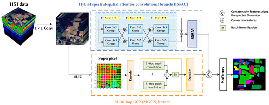
Figure 1.
The MPAS flowchart consists of two branches: the multi-hop GCN and HSSAC.
2.1. Data Preprocessing
In this study, inspired by the network-in-network approach [48], the original HSI data, denoted by (with dimensions representing the spatial dimensions (height and width) and the number of spectral bands), was preprocessed using spectral transformations. Specifically, was sequentially processed through a batch normalization (BN) layer, two 1 × 1 kernel 2D CNN convolutional layers, and a LeakyReLU activation layer, resulting in the processed data . This process promoted robustness and discriminative learning of the spectral features by removing noise and redundant information from the original data.
2.2. Feature Conversion and MGCN
2.2.1. Conversion of Pixels to Superpixels
GCNs only accept graph data as input, and features generated by CNNs are arranged in standard rectangular grids. Although considering individual image pixels as nodes in the graph is possible, this approach would significantly increase the number of nodes involved, leading to high computational complexity in subsequent adjacency matrix calculations. To overcome this challenge, we employed a simple linear iterative clustering (SLIC) [49] algorithm to group the pixels into visually meaningful superpixels, which were then used as nodes in the graph structure. Due to the varying number of pixels in each superpixel, the segmentation method mentioned above cannot be directly integrated into our proposed MPAS framework. Drawing inspiration from Liu et al. [42], we applied data structure conversion to facilitate feature propagation between the pixels and superpixels, as illustrated in Figure 2.
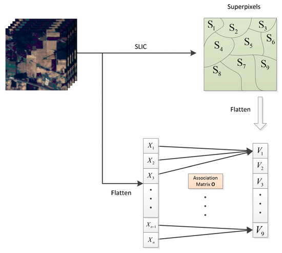
Figure 2.
Flow chart of the encoder; denotes the ith pixel in the flattened HSI and denotes the centroid of the jth superpixel .
Specifically, let denote the association matrix between the pixels and superpixels, where Z represents the number of superpixels[M1]. , is the segment scale of a superpixel.
The association matrix between the pixels and superpixels was constructed by Equation (2):
Here, Flatten(·) signifies the operation to flatten the HSI data along the spatial dimensions. The value of O at position is denoted by ; denotes the i-th pixel in and denotes the jth superpixel. To implement feature transformation, we can use the following formula:
Here, represents O normalized by column. V represents nodes composed of superpixels and Reshape(·) denotes the operation of restoring the spatial dimensions of the flattened data. represents the features transformed back to the grid. After applying SLIC segmentation, the features can be considered nodes in an undirected graph, denoted as G = (V, E), where V refers to the set of nodes and E refers to the set of edges. In this case, the nodes’ features represent the average values of the pixel features within the corresponding superpixels.
We used a graph encoder to convert the grid features to node features, and a graph decoder to assign the node features back to pixels. The network could integrate the graph encoder and decoder, thus leveraging the strengths of CNNs and GCNs.
2.2.2. MGCN
In a single-layer GCN, the nodes aggregate features from their nearest-neighbor nodes and update their information through the adjacency matrix A. In addition, the improved GCNs are constructed by expanding the network layers, leading to a significant increase in the convolutional operations’ complexity and parameters as the network depth grows, which may lead to overfitting or degradation of the network performance; therefore, constructing parallel multi-hop graphs is an effective strategy to enhance the discriminative capacity of features and capture a broader range of receptive fields, leading to improved performance of the graph convolution. Figure 3 depicts the construction process of the parallel multi-hop graph structure.
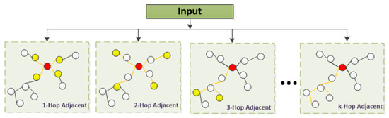
Figure 3.
Parallel multi-hop diagram structure diagram.
For a given graph , the adjacency matrix can be expressed as
where and denote the features of the node , and is the k-hop neighbor of the node .
The parameter is an empirical set. In our approach, we can achieve multi-scale operations by aggregating different hops of neighbors. In MGCN, the lth layer of the 1-hop graph convolution can be calculated as follows:
is the normalized layer output, is the adjacency matrix of the aggregated 1-hop neighbors, is the degree matrix of , is the trainable weight matrix of lth layer of the one-hop graph convolution, and denotes the activation function.
Similar to the equation above, the output of the lth layer of the k-hop graph convolution can be expressed as:
In summary, we utilized an encoder module to transform the grid features into node features, facilitating the seamless integration of GCNs into the CNNs framework. Multi-hop graphs enabled the extraction of multi-scale superpixel-level features from large adjacent regions. Subsequently, the decoder module performed an inverse transformation on the node features to accomplish pixel-level classification tasks. We applied a normalization layer to normalize the output features to ensure stable final outputs. Consequently, the proposed approach effectively integrates GCNs and CNNs for HSI classification, leveraging the strengths of each method to achieve improved performance.
2.3. HSSAC
2.3.1. MSSC
The 2D CNN has a powerful contextual information acquisition capability, formulated [50] as:
In the proposed model, represents the location of the output data layer of the HSI. denotes the specific value of the feature mapping at the (l − 1) layer for the position . represents the value of the convolution kernel at position (h, w) at the lth layer; here, H represents the height and W represents the width of the kernel. bl indicates the bias of the lth layer and σ(·) denotes the activation function used in MPAS, LeakyReLU.
To enhance the capability of CNN-based networks to capture features and overcome the limitation of a single fixed kernel with a limited receptive field, we proposed the MSSC module. The MSSC module was crucial in expanding the network’s capacity to capture diverse multi-scale features.
Upon entering the MSSC module, the HSI data underwent BN to adjust the distribution at each convolutional layer unit. This step prevented overfitting and accelerated the network training. We devised a parallel multi-scale spectral–spatial information extraction network with kernels of different sizes to enhance the feature acquisition capabilities of CNN-based networks and overcome the limitations of a single fixed kernel’s receptive field. Specifically, the two parallel paths in this network employed convolutional kernels with sizes of m = 5 and 3, respectively. Since HSI are rich in spectral information, directly applying 2D CNNs with different kernels to HSIs will result in 2D CNNs with different kernels, which may not be flexible in weighting and adjusting the features of different bands. Then, the importance of specific bands may be underestimated or overestimated, resulting in the degradation of the model’s handling of HSIs, which weakens the network’s classification performance. The MSSC module thus employed independent convolutional layers, including 1 × 1 pointwise convolutional layers and parallel m × m convolutional layers. After 1 × 1 pointwise convolution layers, the features were obtained:
where denotes the value of channel k at position (x, y) in the output feature map (layer l), denotes the value of channel k at position (x, y) in the input feature map (layer l − 1), denotes the weight of the kth channel in the pointwise convolution kernel (layer l), denotes the bias of the lth layer, and σ(·) denotes the activation function.
In MSSC, we employed cross-path fusion to integrate the features extracted by different-scale convolutional kernels for the input of the subsequent convolutional layer. Traditional multi-path multi-scale CNN networks treat each branch as relatively independent and merge the features captured by each branch at the final stage; however, an information disparity exists between the information at large and small scales, restricting the network’s feature fusion capability. In contrast, for the input , we iteratively introduced cross-path connections between the two convolutional paths with kernel sizes of m, facilitating comprehensive integration of the convolutional modules that captured large-scale and small-scale information before advancing to the subsequent layer.
where and denote the convolution kernel sizes m = 3 and 5, respectively.
We facilitated the subsequent cross-path fusion and output by employing convolutional kernels of different sizes and utilizing padding operations to match the spatial resolution of the features. The cross-path connections allowed for integrating large-scale semantic information and small-scale precision information. The higher-level information influenced and directed the feature extraction process of the lower-level paths, while the lower-level information complemented the higher-level path’s semantic representation, reducing information discrepancies that exist between large-scale and small-scale information caused by the feature extraction process.
Following the three-stage convolution using MSSC, the features obtained from the three branches, , , and , were concatenated for subsequent fusion in the succeeding modules.
where ⊕ denotes the operation of contact. and denote the output of parallel m × m convolution, respectively, and T denotes the output of 1 × 1 pointwise convolution.
2.3.2. SSAM
In order to improve the performance and accuracy of the model and reduce the interference of useless features, we drew inspiration from the CBAM attention mechanism and designed SSAM to optimize the feature extraction and classification performance of the model while reducing the amount of computation [51]. The SSAM module performed a weighted fusion of HSIs’ spatial and spectral features, which adaptively selects useful features while reducing the amount of computation, improves the model’s attention to informative features, and captures finer spectral–spatial information.
The SSAM model works as shown in Figure 4:
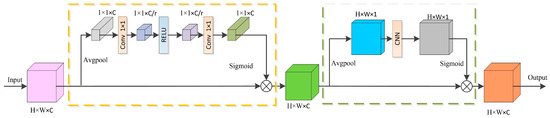
Figure 4.
Spectral–spatial attention mechanism structure diagram.
- Channel attention
Given a feature map M with a shape of H × W × C, we applied global average pooling to obtain a channel description of shape 1 × 1 × C, capturing the global information of each channel. Subsequently, the channel descriptions were input into a 1 × 1 convolutional layer for further processing, resulting in a feature vector of shape 1 × 1 × (C/r), where r represented the scaling factor. We utilized the ReLU activation function to activate the feature vector.
Next, the feature vector underwent another 1 × 1 convolutional layer, followed by an activation function to adjust the weights further. Through this process, we obtained channel weight coefficients of shape 1 × 1 × C. Finally, we multiplied the weight coefficients element-wise with the original input feature map M to obtain the final output feature map. The formula was
The output features of the channel attention are represented by the variable ; Avgpool(·) denotes the average pooling; and denotes the convolutional layer with kernel 1 × 1. ReLU(·) and Sigmoid(·) denote the activation function.
By employing the operations above, we effectively implemented a channel attention mechanism to learn and adjust each channel’s importance weights in the feature map. This mechanism enhanced crucial channel representations, emphasizing their contribution to the overall feature expression.
- 2.
- Spatial attention
The feature extracted from the channel attention mechanism (12) had a shape of H × W × C. We employed channel-wise global average pooling to convert it into a spatial description of shape H × W × 1, enabling the capture of global information for each channel across the entire spatial domain. Subsequently, the spatial description was fed into a k × k convolutional layer to learn the pixel-wise weights, which were further adjusted using an activation function. The obtained spatial weights were then multiplied element-wise with the original input feature map, resulting in the final output feature map.
where denotes the output features of the spatial attention mechanism; Avgpool(·) denotes the average pooling; denotes the convolutional layer with a kernel size of k × k, where we set k to 5; and Sigmoid(·) denotes the activation function.
The SSAM module effectively integrates global channel information and pixel weighting, which enhances the feature representation. It captures the significance of each channel in the entire spatial range, effectively extracting and enhancing key features in HSIs while reducing unnecessary computational complexity and ensuring the accuracy and robustness of HSI classification.
2.4. Feature Fusion and Classification (FFAC)
Our methodology utilized a dual-branch network architecture: MGCN and HSSAC. The MGCN branch employed a multi-hop graph to efficiently extract multi-scale superpixel information by aggregating features of distant neighbor nodes to capture structural information in HSIs. HSSAC extracted multi-scale pixel-level features to compensate for the superpixel-based methods, further improving classification accuracy by considering pixel-level detail information. Owing to the distinct neural network models employed in the two branches, there were noticeable differences in the feature distributions. Consequently, we performed a concatenation operation to fuse the features derived from the dual branches.
Here, Y represents the output of multi-feature fusion and Cat(·) represents the concatenation operation. and represent the output of the MGCN and HSSAC branches, respectively.
For network training, the loss function can be formulated using cross-entropy.
In the equation, R represents the ground-truth labels, P represents the predicted values for each pixel, denotes the d-th element of the label R, and represents the probability that pixel i belongs to class d, obtained using the softmax function. D represents the total number of classes and U represents the total number of samples in the training dataset.
3. Experiments
This section details the experimental results, our interpretation of them, and our conclusions.
3.1. Data Description
For our experimental evaluation, we utilized three well-known benchmarks for HSI datasets: Indian Pines (IP), WHU-Hi-LongKou (LK), and Salinas (SA). These datasets were chosen to assess the performance of the proposed MPAS.
3.1.1. IP
The IP dataset, acquired in 1992 using the airborne visible/infrared imaging spectrometer (AVIRIS) sensor, is among the pioneering HSI datasets employed for classification purposes [30]. This dataset comprises an image with a spatial resolution of 20 m × 20 m, encompassing 145 × 145 pixels. It has a wavelength range from 0.4 μm to 2.5 μm, comprising 220 contiguous spectral bands. Out of 21,025 pixels, approximately half (10,366 pixels) are assigned labels from a set of 16 different classes. For each class, we performed a random selection in which 10% of the samples were allocated for training, 1% for validation, and 89% for testing. Table 1 shows a detailed breakdown of the classes and dataset division.

Table 1.
Number of pixels within the training and test sets for all categories of IP.
3.1.2. LK
The LK dataset was collected on 17 July 2018, between 13:49 and 14:37, in Longkou Town, Hubei Province, China. A DJI Matrice 600 Pro (DJI M600 Pro) drone platform with a Headwall Nano-Hyperspec image sensor with an 8-mm focal length was used to acquire the data. Six crops, including corn, cotton, sesame, broad-leaf soybean, narrow-leaf soybean, and rice, were grown in the research region. The UAV captured an HSI with a resolution of roughly 0.463 m per pixel and an image size of 550 × 400 pixels. It has 270 bands, with wavelengths ranging from 400 to 1000 nm. Throughout the data collection, the UAV was in flight at an altitude of 500 m. We chose 0.1% of the samples at random for training, 0.1% for validation, and 99.8% for testing for each class. A thorough description of the classifications and dataset partition is provided in Table 2.
Table 2.
Number of pixels within the training and test sets for all categories of LK.
3.1.3. SA
The SA dataset was obtained using the AVIRIS sensor in the SA Valley, California, the United States. It consists of an image with dimensions of 512 × 217 pixels and a spatial resolution of 3.7 m. The dataset comprises 224 spectral bands, covering a wavelength range of 360 to 2500 nm. The SA dataset includes 16 land cover categories and 54,129 labeled samples. For each class, we randomly selected 1% of the samples for training, 1% for validation, and 98% for testing. Table 3 shows a detailed breakdown of the classes and dataset division.
Table 3.
Number of pixels within the training and test sets for all categories of SA.
3.2. Experimental Settings and Assessment Criteria
The training and inference stages were performed using Python 3.7 and PyTorch 1.10.0 [52] on a high-performance computer with a GeForce RTX 3060 and an AMD Ryzen 7 3700X 8-Core Processor with 24 GB of memory.
The training samples were collected through random sampling for the IP, LK, and SA datasets since the labeled data were not pre-divided into training and testing sets. The remaining data were utilized as test samples. The parameters were randomly initialized in the training phase, and the MPAS was trained using the Adam optimizer for 300 epochs. The learning rate was 0.0005.
To evaluate the performance of MPAS, we used three metrics: overall accuracy (OA), average accuracy (AA), and the kappa coefficient (Kappa). OA is the proportion of accurately predicted testing pixels to the total number of testing pixels, while AA refers to the average accuracy across all categories. Kappa is a statistical metric to assess the agreement or consistency between classification results and the ground truth. Greater values of these metrics indicate improved classification performance.
3.3. Classification Results
We compared our MPAS algorithm with seven advanced DL methods to demonstrate its effectiveness. These methods included DBDA [53], DBMA [54], FDSSC [55], SSFTT [35], DMSGer [47], WFCG [43], and CEGCN [42]. WFCG, DMSGer, and CEGCN use graph-based neural networks for HSI feature extraction. Each experiment was conducted 10 times, and the average values of the evaluation metrics (OA, AA, and Kappa) were reported. Table 4, Table 5 and Table 6 display the algorithms’ classification accuracy and runtime on different datasets. The classification results of the different methods for the three datasets are listed, and the highest values in each row are marked in bold to highlight the performance. The classification plots on the three datasets are shown in Figure 5, Figure 6 and Figure 7.
Table 4.
The classification accuracy (%) of various methods on the IP dataset with the corresponding class names from Table 1.
Table 5.
The classification accuracy (%) of various methods on the LK dataset and the corresponding class names, as listed in Table 2.
Table 6.
The classification accuracy (%) of various methods on the SA dataset and the corresponding class names from Table 3.
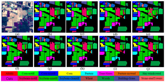
Figure 5.
Classification maps on the IP dataset. (a) False-color image; (b) ground truth; (c) DBDA (97.79%); (d) DBMA (97.21%); (e) FDSSC (97.44%); (f) SSFTT (98.45%); (g) DMSGer (98.55%); (h) CEGCN (98.32%); (i) WFCG (97.91%); (j) MPAS (99.24%).
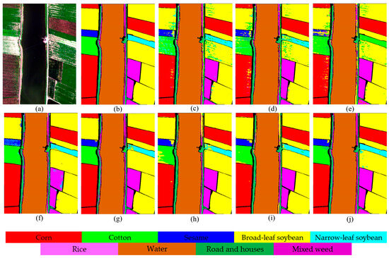
Figure 6.
Classification maps on the LK dataset. (a) False-color image; (b) ground truth; (c) DBDA (93.63%); (d) DBMA (93.67%); (e) FDSSC (93.09%); (f) SSFTT (97.08%); (g) DMSGer (98.17%); (h) CEGCN (96.62%); (i) WFCG (97.54%); (j) MPAS (98.89%).
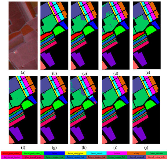
Figure 7.
Classification maps on the SA dataset. (a) False-color image. (b) Ground truth. (c) DBDA (93.60%). (d) DBMA (95.48%). (e) FDSSC (96.72%). (f) SSFTT (98.01%). (g) DMSGer (99.07%). (h) CEGCN (99.35%). (i) WFCG (98.76%). (j) MPAS (99.66%).
3.3.1. IP
Table 4 demonstrate that our MPAS outperformed all other methods regarding the three evaluation metrics. Notably, it achieved 100% accuracy for three land cover categories (alfalfa, pasture, and pasture-mowed) and excellent accuracy for the others.
Among the compared methods, FDSSC, DBMA, and DBDA use complex frameworks, such as 3D CNN, residual connections, and dense connections, to improve the network performance, resulting in significantly increased computational cost and training time. Although SSFTT uses a lightweight network architecture, it performed poorly in some categories with fewer samples, such as categories 7 and 16. WFCG and CEGCN have fixed-neighbor graph structures; with those methods, it was challenging to effectively represent the relationships between the imbalanced nodes. DMSGer uses dynamic graph convolution to handle information at different scales but is still limited to single-hop graph convolution, whereas multi-hop graph convolution can further enhance the model’s ability to perceive node relationships over a wider range of nodes, thus enhancing feature representation. Additionally, WFCG has a relatively higher computational cost due to its complex network structure. Compared to DMSGer, WFCG, and CEGCN, our MPAS improves 0.69%, 1.33%, and 0.92% in OA, 1.32%, 2.62%, and 2.67% in AA, and 0.78%, 1.22%, and 1.05% in Kappa, respectively. These empirical results demonstrate that MPAS is a robust and reliable classifier for HSI classification.
For clarity, we provided the ground truth of the IP dataset and reported the OA values of different methods. Among the first four DL-based methods (FDSSC, DBMA, DBDA, and SSFTT), certain areas were still visibly misclassified, even though the classification maps generated by these methods exhibited overall similarity and accuracy. This misclassification may be due to the fact that these methods primarily emphasize analyzing local pixel relationships rather than considering long-range dependencies. The three graph-based methods’ misclassified areas were smaller than in most DL-based methods. Due to GCNs’ global feature extraction capability, they can effectively capture relevant information over lengthier distances within the structure. Compared with DMSGer, CEGCN, and WFCG, our MPAS provides a more realistic interpretation of HSI, captures relationships between nodes at longer distances, and improves the performance of the model through multi-scale feature fusion and cross-layer information transfer.
3.3.2. LK
The lower classification accuracy of DBDA, DBMA, and FDSSC illustrates the weakness of DL-based methods when handling fewer HSI samples. The classification performance of SSFTT can be equal to that of GCN-based methods, which is due to the fact that the transformer can fully exploit the long-range dependencies of the samples to improve the classification accuracy. For GCN-based methods (CEGCN, WFCG and DMSGer), it is difficult to achieve the expected classification performance due to the inability to integrate the multi-scale pixel-level and superpixel-level fusion information well. MPAS can achieve the best results of OA, AA, and Kappa at a certain time cost. We can also see from Figure 6 that the MPAS method produced classification maps that closely approximated the ground truth map.
3.3.3. SA
Similar to the other datasets, MPAS achieved the highest OA, AA, and Kappa values. Notably, MPAS achieved a maximum accuracy of 100% in the following categories: brocoli_green_weeds_2, soil_vineyard_develop, lettuce_romaine_5wk, and lettuce_romaine_6wk. It also exhibited excellent accuracy for the other land cover classifications. MPAS demonstrated significant advantages in both performance and stability compared to the existing four DL-based methods. The finding above highlights MPAS’s efficacy for the HSI classification task. Figure 7 displays the ground truth and predicted classification maps obtained by various methods on the SA dataset. Although the classification maps produced by the four DL-based methods were of good quality, the limited training samples prevented them from reaching the expected level of accuracy. For the three graph-based methods (CEGCN, DMSGer, and WFCG), there were scattered errors in some areas in the upper-left corner and the middle-right area due to insufficient extraction of edge information. MPAS utilizes different levels of feature representations to improve the modeling of feature edges.
In comparison, the classification map generated by MPAS demonstrated accuracy and closely resembled the ground truth map.
4. Discussion
4.1. Effectiveness of Different Modules in MPAS
Table 7 presents the results of ablation experiments performed on the IP dataset. The experimental results evidence that every model component functioned to enhance its overall performance. Specifically, the comparison between (1), (2), and (3) revealed the positive impact of each module in MPAS on the classification performance. The combination of MSSC and SSAM in the HSSAC branch, as indicated by (2), (3), and (4), enhanced and improved the feature extraction of HSI. The performance of the combined branches (5) and (6) also surpassed that of the individual branches. Although the expected classification results were not achieved due to insufficient extraction of pixel-level spectral–spatial features, the collaborative efforts of the four modules in MPAS, as evident from (7), improved the classification performance, further confirming our proposed method’s efficacy. Figure 8 demonstrates the classification accuracy of MPAS at the superpixel level and pixel level. From the illustration, it can be seen that simply extracting pixel-level or superpixel-level features causes the problem of loss of spatial context information and loss of fine-grained information, and combining these two levels of features can better capture the spatial context information. The experimental results provide strong evidence supporting each module’s effectiveness in MPAS, as they contributed to generating more accurate classification maps.
Table 7.
Ablation experiments of modules on the IP dataset.
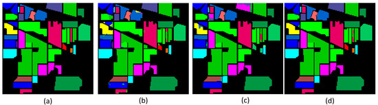
Figure 8.
Classification maps at the pixel and superpixel level. (a) Ground truth; (b) pixel level (96.34%); (c) superpixel level (94.65%); (d) MPAS (99.12%).
4.2. Effectiveness of Attention Mechanisms
In order to verify the effect of the SSAM module in this study, we conducted experiments on each of the three datasets by adding SSAM and the traditional CBAM module into the framework of this paper, respectively, comparing their OA and training time by performing each experiment 10 times and averaging them. Figure 9 shows a significant reduction in the training time and improvement in the classification performance of SSAM compared to the traditional CBAM attention mechanism. The SSAM module saves training time and computational resources while maintaining high classification performance.
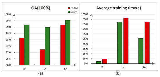
Figure 9.
The figure shows the experimental results of the two comparisons of SSAM and CBAM. (a) Classification effects; (b) average training time.
4.3. Hyperparameter Selection
In this experiment, in order to investigate the effects of superpixel segmentation scale λ, the maximum epoch number, the number of hops in the convolution of a multi-hop graph k, and learning rate Lr on the model performance. The hyperparameters were set as shown in Table 8. We used a grid search strategy to find the optimal settings. OA was utilized to show the performance of MPAS with different parameter settings.
Table 8.
Hyperparameter settings.
4.3.1. Effectiveness of Splitting Scale
When constructing the graph using the SLIC algorithm, the segmentation scale λ was crucial in determining the correspondence between the pixels and superpixels. The choice of λ directly impacted the number of pixels assigned to each superpixel, affecting the resulting graph’s size and structure. To investigate this, we conducted experiments using different values of λ (100, 200, 300, 400, and 500) and evaluated the classification accuracy on each dataset. Each experiment was repeated 10 times. Figure 10 presents the average values of the metrics.
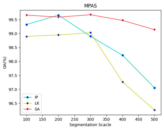
Figure 10.
OAs under different λ values on each dataset.
On the IP dataset, MPAS demonstrated a more pronounced decline in performance as the segmentation scale increased, in contrast to the other two datasets. We attributed this finding to the limited size of the IP dataset, which has a relatively dense distribution of land cover and similar land cover types. In contrast, the LK dataset displays more differences in land cover, leading to overall performance stability. Additionally, the SA dataset’s classification results for similar land cover types are smoother due to the larger number of pixels in the superpixel nodes.
Consequently, there is a slight improvement in the classification performance from λ = 100 to λ = 300; however, increasing λ beyond 400 leads to a decrease in OA with each pixel node’s addition. To prevent MPAS from producing excessively smooth classification maps, we fixed λ at 100 for all the experiments.
4.3.2. Effectiveness of Lr and Epoch Selection
The experiment extensively explored the sensitivity of Lr and epoch, examining their effects on the MPAS model in detail. To analyze the impacts of these two parameters, a fixed value of 100 was assigned to λ. Lr was set to 0.05, 0.01, 0.005, and 0.0001. The value of the epoch varied between 100 and 500, and the interval was 100. Figure 11 illustrates the variations in OA values across different parameter combinations for the three datasets. It can be seen from the results that the proposed method achieves the best accuracy when the epoch is set to 500 on IP. For LK datasets and SA, setting the epoch to 300 is the best choice; however, increasing the epoch size leads to a proportional increase in the time required for model training. Regarding Lr, employing a larger value can expedite the training of the model parameters; however, it may hinder the attainment of optimal parameters. Conversely, opting for a smaller Lr necessitates a longer training time for the model but enhances the chances of achieving optimal parameters. With a focus on achieving optimal classification accuracy and learning efficiency, the method employed in this paper establishes the Lr value as 0.0005.
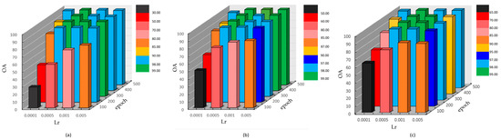
Figure 11.
Effect of Lr and epoch for MPAS. (a) IP; (b) LK; (c) SA.
4.3.3. Effectiveness of K Value
To examine the effect of different values of the number of hops (k) on the HSI classification performance in the multi-hop graph convolution, we conducted experiments on the IP dataset with k-values ranging from 1 to 5. This experiment aimed to comprehensively explore the effect of the k-value selection on the HSI classification performance and provide guidance for optimizing subsequent algorithms.
As Figure 12 shows, the performance of HSI classification exhibits an initial increase followed by a decrease as the k-value increases because smaller k-values allow the multi-hop graph convolution to capture local spatial information, leading to improved performance in HSI classification. As k increases, the graph convolution can obtain information from farther nodes, helping to better capture broader contextual information; however, continuing to increase the number of hops may introduce excessive noise and reduce the classification performance. Additionally, as the number of hops increases, the number of parameters also increases, which may cause overfitting of the model to the training data. We chose k = 3 in this study to reduce overfitting and the computational cost.
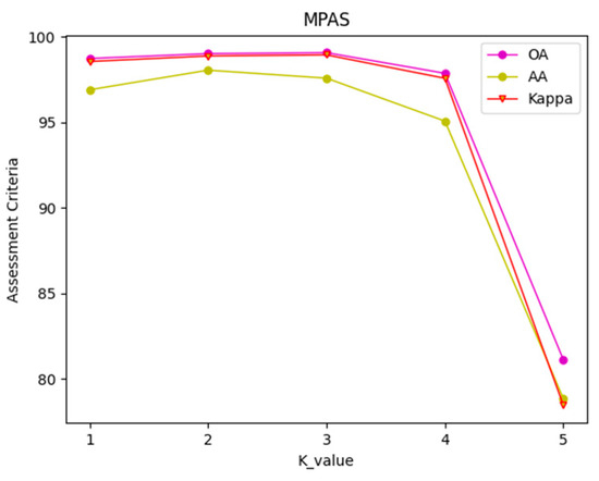
Figure 12.
K-value changes on the IP dataset.
4.4. Effectiveness of Training Samples
Considering the high cost in terms of human and time resources associated with labeling, an HSI classification model’s ability to learn from small samples is crucial for its practical applicability. To evaluate the effectiveness of the proposed MPAS method, we conducted a performance assessment when the training samples were minimal. Specifically, we studied its classification accuracy and compared it with other competitors at different labeled sample sizes. The training sample ratios of the IP dataset were set to 1%, 3%, 5%, 7%, and 10% per class, while those of the LK and SA datasets were set to 0.1%, 0.3%, 0.5%, 0.7%, and 1% per class. The experimental results demonstrate that the proposed MPAS algorithm consistently achieved the highest classification accuracy across all three datasets and that the OA monotonically rose with the training sample size’s increase, demonstrating its strong small sample learning ability. Figure 13 depicts the results of the experiments.
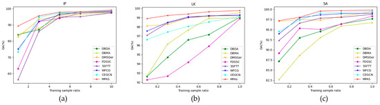
Figure 13.
Classification accuracies of different methods under different scales of training samples. (a) IP; (b) LK; (c) SA.
The same sensor generated the SA and IP datasets, yet their distributions differ significantly. Specifically, the IP dataset suffers from severe class imbalance, making it a more challenging source for classification than the SA dataset, especially when the available labeled data are limited. Fortunately, MPAS exhibits acceptable performance on both datasets, underscoring its utility for HSIs classification tasks. Nevertheless, mitigating the impact of class imbalance on classification accuracy remains a crucial research pursuit.
4.5. Effectiveness of Convolutional Kernel
In the MSSC module, we used two parallel m × m convolution kernels to capture the multi-scale spectral–spatial information of HSIs. We chose the sizes of these two convolution kernels to be 3 (i.e., 3 × 3), 5 (i.e., 5 × 5), and 7 (i.e., 7 × 7). There are three combinations: (3,5), (3,7), and (5,7). The numbers in parentheses indicate the respective kernel sizes used in the first and second layers. Based on the results shown in Figure 14, the kernel size of (3,7) achieves the highest performance on all three datasets; the average classification effect is 0.24% and 0.60% higher than that of (3,5) and (5,7) for the IP dataset, for example. Given the considerations of both the training and inference speed of the model, we used a convolutional kernel size of (3,5) in our experiments.
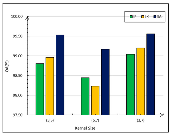
Figure 14.
The graph shows the relationship between the sizes of the OA and the convolutional kernel. Three combinations of kernel sizes are considered: (3,5), (3,7), and (5,7). In the (3,5) combination, the first convolutional layer utilizes a kernel size of 3 × 3, while the second convolutional layer employs a kernel size of 5 × 5.
4.6. Computational Efficiency
In this section, we verify the computational efficiency by observing the inference time cost and model size of MPAS using the IP dataset. As shown in Table 9, MPAS ensures efficient training time and small memory cost while guaranteeing classification performance. The computation time of MPAS is 9.16 s and the model size is only 0.78 MB. These observations confirm the efficiency of MPAS. The reason behind this is twofold. In order to efficiently reduce computational and storage overheads, parallel multi-hop graph convolution can quickly aggregate context information from various locations. On the other hand, the HSSAC module’s simplified design reduces the computational complexity and conserves space; therefore, our MPAS is a lightweight and time-saving HSI classification model.
Table 9.
Computational complexity analysis on IP datasets.
5. Conclusions
This study proposes a multiscale pixel-level and superpixel-level (MPAS)-based classification method for HSI. The network consists of two sub-networks, namely, HSSAC and MGCN, and a feature fusion module. HSSAC comprehensively captures pixel-level features with different kernel sizes through parallel multi-scale convolution and cross-path fusion to reduce the semantic information loss caused by fixed convolution kernels during feature extraction, and learns adjustable weights from the adaptive spectral–spatial attention module (SSAM) to capture pixel-level feature correlations. MGCN efficiently captures structural information in HSI data by building cascade networks using parallel multi-hop GCNs. The proposed MPAS can efficiently aggregate multi-layer contextual features from spectral–spatial information at the pixel and superpixel levels, enhancing the HSI classification task. Evaluation experiments on three benchmark HSI datasets show that the MPAS has robust feature-learning and feature-fusion capabilities compared to other advanced networks. Our future research will primarily concentrate on enhancing the network architecture, particularly emphasizing deep-feature fusion to enhance the model’s training efficiency and classification accuracy.
Abbreviation
The abbreviations for all key terms in this article are explained below:
| CNNs | Convolutional neural networks |
| GCNs | Graph convolutional networks |
| LBP | Local binary pattern |
| MPAS | Multiscale pixel-level and superpixel-level method |
| HSSAC | Hybrid spectral–spatial attention convolution branch |
| MGCN | Multi-hop graph convolution branch |
| SSAM | Adaptive spectral–spatial attention module |
| SSFTT | Spectral–spatial feature-tagging transformer |
| CEGCN | CNN-enhanced GCN |
| WFCG | Weighted feature fusion network |
| DMSGer | Dynamic multi-scale graph dialogue network |
| SLIC | Simple linear iterative clustering |
| IP | Indian Pines |
| LK | WHU-Hi-LongKou |
| SA | Salinas |
| AA | Average accuracy |
| OA | Overall accuracy |
| Kappa | Kappa coefficient |
Author Contributions
Methodology, software, and conceptualization, J.Y., X.L. and R.H.; modification and writing—review and editing, Q.C., W.H. and A.L.; validation, P.W. All authors have read and agreed to the published version of the manuscript.
Funding
This study was supported by the National Natural Science Foundation of China (Grant No. 32271880) and the Henan Province Science and Technology Breakthrough Project (Grant No. 232102211048).
Data Availability Statement
The data presented in this study are available in the article.
Acknowledgments
The authors would like to thank the editors and reviewers for their advice.
Conflicts of Interest
The authors declare no conflict of interest.
References
- Wambugu, N.; Chen, Y.; Xiao, Z.; Tan, K.; Wei, M.; Liu, X.; Li, J. Hyperspectral image classification on insufficient-sample and feature learning using deep neural networks: A review. Int. J. Appl. Earth Obs. Geoinf. 2021, 105, 102603. [Google Scholar] [CrossRef]
- Jia, S.; Jiang, S.; Lin, Z.; Li, N.; Xu, M.; Yu, S. A survey: Deep learning for hyperspectral image classification with few labeled samples. Neurocomputing 2021, 448, 179–204. [Google Scholar] [CrossRef]
- Yang, J.; Du, B.; Zhang, L. From center to surrounding: An interactive learning framework for hyperspectral image classification. ISPRS J. Photogramm. Remote Sens. 2023, 197, 145–166. [Google Scholar] [CrossRef]
- Zhang, Y.; Li, W.; Sun, W.; Tao, R.; Du, Q. Single-source domain expansion network for cross-scene hyperspectral image classification. IEEE Trans. Image Process. 2023, 32, 1498–1512. [Google Scholar] [CrossRef]
- Duan, Y.; Luo, F.; Fu, M.; Niu, Y.; Gong, X. Classification via structure-preserved hypergraph convolution network for hyperspectral image. IEEE Trans. Geosci. Remote Sens. 2023, 61, 5507113. [Google Scholar] [CrossRef]
- Li, X.; Liu, B.; Zhang, K.; Chen, H.; Cao, W.; Liu, W.; Tao, D. Multi-view learning for hyperspectral image classification: An overview. Neurocomputing 2022, 500, 499–517. [Google Scholar] [CrossRef]
- Liang, N.; Duan, P.; Xu, H.; Cui, L. Multi-view structural feature extraction for hyperspectral image classification. Remote Sens. 2022, 14, 1971. [Google Scholar] [CrossRef]
- Li, S.; Song, W.; Fang, L.; Chen, Y.; Ghamisi, P.; Benediktsson, J.A. Deep learning for hyperspectral image classification: An overview. IEEE Trans. Geosci. Remote Sens. 2019, 57, 6690–6709. [Google Scholar] [CrossRef]
- Dong, Y.; Liang, T.; Zhang, Y.; Du, B. Spectral–spatial weighted kernel manifold embedded distribution alignment for remote sensing image classification. IEEE Trans. Cybern. 2020, 51, 3185–3197. [Google Scholar] [CrossRef]
- Luo, F.; Zhou, T.; Liu, J.; Guo, T.; Gong, X.; Ren, J. Multiscale diff-changed feature fusion network for hyperspectral image change detection. IEEE Trans. Geosci. Remote Sens. 2023, 61, 5502713. [Google Scholar] [CrossRef]
- Sun, H.; Zheng, X.; Lu, X.; Wu, S. Spectral–spatial attention network for hyperspectral image classification. IEEE Trans. Geosci. Remote Sens. 2019, 58, 3232–3245. [Google Scholar] [CrossRef]
- Zhou, W.; Kamata, S.I.; Wang, H.; Xue, X. Multiscanning-Based RNN-Transformer for Hyperspectral Image Classification. IEEE Trans. Geosci. Remote Sens. 2023, 61, 1–19. [Google Scholar] [CrossRef]
- Tang, P.; Zhang, M.; Liu, Z.; Song, R. Double Attention Transformer for Hyperspectral Image Classification. IEEE Geosci. Remote Sens. Lett. 2023, 20, 5502105. [Google Scholar] [CrossRef]
- Yue, J.; Fang, L.; Rahmani, H.; Ghamisi, P. Self-supervised learning with adaptive distillation for hyperspectral image classification. IEEE Trans. Geosci. Remote Sens. 2021, 60, 1–13. [Google Scholar] [CrossRef]
- Xie, E.; Chen, N.; Peng, J.; Sun, W.; Du, Q.; You, X. Semantic and spatial–spectral feature fusion transformer network for the classification of hyperspectral image. CAAI Trans. Intell. Technol. 2023. [Google Scholar] [CrossRef]
- Zhang, M.L.; Zhou, Z.H. ML-KNN: A lazy learning approach to multi-label learning. Pattern Recognit. 2007, 40, 2038–2048. [Google Scholar] [CrossRef]
- Xue, W.; Zhang, L.; Mou, X.; Bovik, A.C. Gradient magnitude similarity deviation: A highly efficient perceptual image quality index. IEEE Trans. Image Process. 2013, 23, 684–695. [Google Scholar] [CrossRef]
- Jia, S.; Deng, B.; Zhu, J.; Jia, X.; Li, Q. Local binary pattern-based hyperspectral image classification with superpixel guidance. IEEE Trans. Geosci. Remote Sens. 2017, 56, 749–759. [Google Scholar] [CrossRef]
- Song, T.; Feng, J.; Li, S.; Zhang, T. Color Context Binary Pattern Using Progressive Bit Correction for Image Classification. Chin. J. Electron. 2021, 30, 471–481. [Google Scholar]
- Jia, S.; Zhuang, J.; Deng, L.; Zhu, J.; Xu, M.; Zhou, J.; Jia, X. 3-D Gaussian–Gabor feature extraction and selection for hyperspectral imagery classification. IEEE Trans. Geosci. Remote Sens. 2019, 57, 8813–8826. [Google Scholar] [CrossRef]
- Belgiu, M.; Drăguţ, L. Random forest in remote sensing: A review of applications and future directions. ISPRS J. Photogramm. Remote Sens. 2016, 114, 24–31. [Google Scholar] [CrossRef]
- Wang, Z.; Du, B.; Guo, Y. Domain adaptation with neural embedding matching. IEEE Trans. Neural Netw. Learn. Syst. 2019, 31, 2387–2397. [Google Scholar] [CrossRef]
- Dong, Y.; Shi, W.; Du, B.; Hu, X.; Zhang, L. Asymmetric weighted logistic metric learning for hyperspectral target detection. IEEE Trans. Cybern. 2021, 52, 11093–11106. [Google Scholar] [CrossRef]
- Chen, Y.; Zhao, X.; Jia, X. Spectral–spatial classification of hyperspectral data based on deep belief network. IEEE J. Sel. Top. Appl. Earth Observ. Remote Sens. 2015, 8, 2381–2392. [Google Scholar] [CrossRef]
- Sun, L.; Fang, Y.; Chen, Y.; Huang, W.; Wu, Z.; Jeon, B. Multi-structure KELM with attention fusion strategy for hyperspectral image classification. IEEE Trans. Geosci. Remote Sens. 2022, 60, 1–17. [Google Scholar] [CrossRef]
- Song, T.; Wang, Y.; Gao, C.; Chen, H.; Li, J. MSLAN: A Two-Branch Multidirectional Spectral-Spatial LSTM Attention Network for Hyperspectral Image Classification. IEEE Trans. Geosci. Remote Sens. 2022, 60, 1–14. [Google Scholar] [CrossRef]
- Jiang, J.; Ma, J.; Liu, X. Multilayer spectral–spatial graphs for label noisy robust hyperspectral image classification. IEEE Trans. Neural Netw. Learn. Syst. 2020, 33, 839–852. [Google Scholar] [CrossRef] [PubMed]
- Jiang, J.; Ma, J.; Wang, Z.; Chen, C.; Liu, X. Hyperspectral image classification in the presence of noisy labels. IEEE Trans. Geosci. Remote Sens. 2018, 57, 851–865. [Google Scholar] [CrossRef]
- Feng, Z.; Liu, X.; Yang, S.; Zhang, K.; Jiao, L. Hierarchical Feature Fusion and Selection for Hyperspectral Image Classification. IEEE Geosci. Remote Sens. Lett. 2023, 20, 5501205. [Google Scholar] [CrossRef]
- Chen, Y.; Jiang, H.; Li, C.; Jia, X.; Ghamisi, P. Deep feature extraction and classification of hyperspectral images based on convolutional neural networks. IEEE Trans. Geosci. Remote Sens. 2016, 54, 6232–6251. [Google Scholar] [CrossRef]
- Ghaderizadeh, S.; Abbasi-Moghadam, D.; Sharifi, A.; Zhao, N.; Tariq, A. Hyperspectral image classification using a hybrid 3D-2D convolutional neural networks. IEEE J. Sel. Top Appl. Earth Obs. Remote Sens. 2021, 14, 7570–7588. [Google Scholar] [CrossRef]
- Ge, H.; Wang, L.; Liu, M.; Zhu, Y.; Zhao, X.; Pan, H.; Liu, Y. Two-Branch Convolutional Neural Network with Polarized Full Attention for Hyperspectral Image Classification. Remote Sens. 2023, 15, 848. [Google Scholar] [CrossRef]
- Liang, L.; Zhang, S.; Li, J. Multiscale DenseNet meets with bi-RNN for hyperspectral image classification. IEEE J. Sel. Top. Appl. Earth Obs. Remote Sens. 2022, 15, 5401–5415. [Google Scholar] [CrossRef]
- Roy, S.K.; Manna, S.; Song, T.; Bruzzone, L. Attention-based adaptive spectral-spatial kernel resnet for hyperspectral image classification. IEEE Trans. Geosci. Remote Sens. 2020, 59, 7831–7843. [Google Scholar] [CrossRef]
- Sun, L.; Zhao, G.; Zheng, Y.; Wu, Z. Spectral–spatial feature tokenization transformer for hyperspectral image classification. IEEE Trans. Geosci. Remote Sens. 2022, 60, 1–14. [Google Scholar] [CrossRef]
- Bruna, J.; Zaremba, W.; Szlam, A.; LeCun, Y. Spectral networks and deep locally connected networks on graphs. arXiv 2014, arXiv:1312.6203. [Google Scholar]
- Kipf, T.N.; Welling, M. Semi-supervised classification with graph convolutional networks. arXiv 2016, arXiv:1609.02907. [Google Scholar]
- Wu, F.; Souza, A.; Zhang, T.; Fifty, C.; Yu, T.; Weinberger, K. Simplifying graph convolutional networks. arXiv 2019, arXiv:1902.07153. [Google Scholar]
- Qin, A.; Shang, Z.; Tian, J.; Wang, Y.; Zhang, T.; Tang, Y.Y. Spectral–spatial graph convolutional networks for semisupervised hyperspectral image classification. IEEE Geosci. Remote Sens. Lett. 2018, 16, 241–245. [Google Scholar] [CrossRef]
- Wan, S.; Gong, C.; Zhong, P.; Du, B.; Zhang, L.; Yang, J. Multiscale dynamic graph convolutional network for hyperspectral image classification. IEEE Trans. Geosci. Remote Sens. 2019, 58, 3162–3177. [Google Scholar] [CrossRef]
- Hong, D.; Gao, L.; Yao, J.; Zhang, B.; Plaza, A.; Chanussot, J. Graph convolutional networks for hyperspectral image classification. IEEE Trans. Geosci. Remote Sens. 2020, 59, 5966–5978. [Google Scholar] [CrossRef]
- Liu, Q.; Xiao, L.; Yang, J.; Wei, Z. CNN-enhanced graph convolutional network with pixel-and superpixel-level feature fusion for hyperspectral image classification. IEEE Trans. Geosci. Remote Sens. 2020, 59, 8657–8671. [Google Scholar] [CrossRef]
- Dong, Y.; Liu, Q.; Du, B.; Zhang, L. Weighted feature fusion of convolutional neural network and graph attention network for hyperspectral image classification. IEEE Trans. Image Process. 2022, 31, 1559–1572. [Google Scholar] [CrossRef] [PubMed]
- Sharifi, O.; Mokhtarzadeh, M.; Asghari Beirami, B. A new deep learning approach for classification of hyperspectral images: Feature and decision level fusion of spectral and spatial features in multiscale CNN. Geocarto Int. 2022, 37, 4208–4233. [Google Scholar] [CrossRef]
- Sun, L.; XU, B.; Lu, Z. Hyperspectral Image Classification Based on A Multi-Scale Weighted Kernel Network. Chin. J. Electron. 2022, 31, 832–843. [Google Scholar] [CrossRef]
- Xue, H.; Sun, X.K.; Sun, W.X. Multi-hop hierarchical graph neural networks. In Proceedings of the 2020 IEEE International Conference on Big Data and Smart Computing (BigComp), Busan, Republic of Korea, 19–22 February 2020; pp. 82–89. [Google Scholar]
- Yang, Y.; Tang, X.; Zhang, X.; Ma, J.; Liu, F.; Jia, X.; Jiao, L. Semi-supervised multiscale dynamic graph convolution network for hyperspectral image classification. IEEE Trans. Neural Netw. Learn Syst. 2022; ahead of print. [Google Scholar]
- Lin, M.; Chen, Q.; Yan, S. Network in network. arXiv 2013, arXiv:1312.4400. [Google Scholar]
- Achanta, R.; Shaji, A.; Smith, K.; Lucchi, A.; Fua, P.; Süsstrunk, S. SLIC superpixels compared to state-of-the-art superpixel methods. IEEE Trans. Pattern Anal. Mach. Intell. 2012, 34, 2274–2282. [Google Scholar] [CrossRef] [PubMed]
- Liu, Q.C.; Xiao, L.; Liu, F.; Xu, J.H. SSCDenseNet: A spectral-spatial convolutional dense network for hyperspectral image classification. Acta Electron. Sin. 2020, 48, 751. [Google Scholar]
- Woo, S.; Park, J.; Lee, J.Y.; Kweon, I.S. Cbam: Convolutional block attention module. In Proceedings of the European Conference on Computer Vision (ECCV), Munich, Germany, 8–14 September 2018; pp. 3–19. [Google Scholar]
- Paszke, A.; Gross, S.; Massa, F.; Lerer, A.; Bradbury, J.; Chanan, G.; Chintala, S. Pytorch: An imperative style, high-performance deep learning library. arXiv 2019, arXiv:1912.01703. [Google Scholar]
- Li, R.; Zheng, S.; Duan, C.; Yang, Y.; Wang, X. Classification of hyperspectral image based on double-branch dual-attention mechanism network. Remote Sens. 2020, 12, 582. [Google Scholar] [CrossRef]
- Ma, W.; Yang, Q.; Wu, Y.; Zhao, W.; Zhang, X. Double-branch multi-attention mechanism network for hyperspectral image classification. Remote Sens. 2019, 11, 1307. [Google Scholar] [CrossRef]
- Wang, W.; Dou, S.; Jiang, Z.; Sun, L. A fast dense spectral–spatial convolution network framework for hyperspectral images classification. Remote Sens. 2018, 10, 1068. [Google Scholar] [CrossRef]
Disclaimer/Publisher’s Note: The statements, opinions and data contained in all publications are solely those of the individual author(s) and contributor(s) and not of MDPI and/or the editor(s). MDPI and/or the editor(s) disclaim responsibility for any injury to people or property resulting from any ideas, methods, instructions or products referred to in the content. |
© 2023 by the authors. Licensee MDPI, Basel, Switzerland. This article is an open access article distributed under the terms and conditions of the Creative Commons Attribution (CC BY) license (https://creativecommons.org/licenses/by/4.0/).