Student’s t-Based Robust Poisson Multi-Bernoulli Mixture Filter under Heavy-Tailed Process and Measurement Noises

Abstract

A novel Student’s t-based robust Poisson multi-Bernoulli mixture (PMBM) filter is proposed to effectively perform multi-target tracking under heavy-tailed process and measurement noises. To cope with the common scenario where the process and measurement noises possess different heavy-tailed degrees, the proposed filter models this noise as two Student’s t-distributions with different degrees of freedom. Furthermore, this method considers that the scale matrix of the one-step predictive probability density function is unknown and models it as an inverse-Wishart distribution to mitigate the influence of heavy-tailed process noise. A closed-form recursion of the PMBM filter for propagating the approximated Gaussian-based PMBM posterior density is derived by introducing the variational Bayesian approach and a hierarchical Gaussian state-space model. The overall performance improvement is demonstrated through three simulations.

1. Introduction

Multi-target tracking (MTT) aims to jointly estimate the time-varying number of targets and their states under the interference of various noises, false alarms, detection uncertainty, and data association uncertainty [1]. It has been widely used in civilian and military fields such as autonomous driving, air traffic control, missile warning, etc. In the past two decades, a new random finite set (RFS)-based MTT strategy, which models the multi-target state and sensor measurement as two individual RFSs, has been developed to avoid the data association required by the traditional MTT strategy [1,2,3].

The multi-target Bayesian (MTB) filter provides an optimal solution for the RFS-based MTT algorithms. However, due to the existence of multiple integrals, as well as the combinatorial nature stemming from the infinite-dimensional multi-target densities, the MTB filter is computationally intractable, which limits its application [1,2,4]. Recently, various suboptimal solutions have been successively developed, with two of the most well known being the probability hypothesis density (PHD) filter [1,5] and the multi-Bernoulli (MeMBer, MB) filter [6]. The PHD filter propagates the multi-target intensity (first-order statistic of the target RFS), which is computationally tractable but not accurate enough. The MeMBer filter propagates the MB density; however, its cardinality estimation has a certain bias. By introducing additional parameters, many variants, such as the cardinality balanced MeMBer (CBMeMBer) filter [7], $\delta$-generalized labeled MeMBer ($\delta$-GLMB) filter [8], and labeled MeMBer (LMB) filter [9], have been developed. It is worth mentioning that both the $\delta$-GLMB filter and the LMB filter can achieve high tracking accuracy and output target trajectories but at the cost of high computational complexity. In recent years, a new variant called the Poisson multi-Bernoulli mixture (PMBM) filter has been developed [10]. The PMBM filter considers the birth process as a Poisson, which is different from the MB birth in the GLMB and LMB filters. The propagated conjugate prior is the combination of a Poisson point process (PPP) and an MB mixture (MBM), in which the former is the modeling of all targets that have never been detected, and the latter considers all the data association hypotheses and is implemented using the track-oriented multiple hypotheses tracking (TOMHT) formulation [10,11]. The PMBM filter achieves a much higher tracking accuracy compared to the aforementioned filters with a lower computational load, so it is a promising filter [12,13,14,15,16,17].

Conventional RFS-based MTT filters are mostly implemented by applying the standard Kalman filter in multi-target fields, so they are only suitable for the Gaussian process and measurement noises [2]. However, in engineering applications, such as maneuvering target tracking, as well as the presence of burst interference and unreliable sensors, the distributions of these noises are usually heavy-tailed non-Gaussian with many outliers. Compared to Gaussian noise, heavy-tailed noise statistically means a larger uncertainty in positions far from the mean, that is, the probability of target movement or measurement far from the mean is higher than that of Gaussian noise. In this situation, the tracking performance of these conventional filters may break down. To mitigate this, the Student’s t-distribution with naturally heavy-tailed characteristics is employed to model the heavy-tailed noise, but this can make obtaining a closed-form recursion intractable. The variational Bayesian (VB) inference provides a solution to this problem. This approach has been widely used for estimating the unknown covariance [3,17,18,19], in which the VB-LMB [18] and Gaussian inverse-Wishart (IW) mixture LMB (GIWM-LMB) [19] filters were proposed by modeling the unknown measurement covariance as inverse-Gamma and IW distributions, respectively. Using a combination of the VB approach and Student’s t-model, a filter called the VB Kalman filter (VB-KF) [20,21] for single-target tracking (STT) under heavy-tailed measurement noise is proposed. This strategy has been extended to MTT fields [22,23,24,25], but the drawback is that they cannot cope with the heavy-tailed process noise. As a generalization of the ubiquitous Kalman filter, the Student’s t-filter (STF) [26] models the process and measurement noises as Student’s t-distributions with the same degrees of freedom (DOF) and then propagates the Student’s t-based density, which can deal with these two noises in a natural manner. Based on this method, the Student’s t mixture CBMeMBer (STM-CBMeMBer) filter [27], the STM-LMB filter [2], and the STM-GLMB filter [28] are proposed, especially the latter two filters, achieving higher estimation accuracy.

However, the STF-based filters still have inherent shortcomings. First, the moment-matching approximation is introduced to prevent the DOF from increasing in the update step. This approximation can only capture the first two moments so it has a large error. Second, the STF-based filters require that the process and measurement noises have the same DOFs, which is seldom experienced in real-world scenarios [26]. Finally, compared to the Gaussian approximation of a posterior probability density function (PDF), the STF-based filters use Student’s t-distribution to approximate the posterior PDF, which proves to be unreasonable [29]. To avoid these drawbacks, a novel heavy-tailed-noise Kalman filter, which models these two noises as Student’s t-distributions with different DOFs, has been proposed to perform STT [29]. This filter uses the hierarchical Gaussian state-space model to approximate the posterior PDF. By introducing the VB approach, the target state is estimated iteratively, and the tracking performance is greatly improved.

To the best of our knowledge, the proposed R-ST-PMBM filter is the first efficient MTT filter that can theoretically handle process and measurement noises with different heavy-tailed degrees. Firstly, to match the characteristics of the heavy-tailed process and measurement noises, the one-step predicted PDF and measurement likelihood PDF are modeled as Student’s t-distributions, where the DOFs can be set inconsistently to cope with process and measurement noises with different heavy-tailed degrees. Secondly, due to the influence of heavy-tailed process noise, it is not possible to obtain an accurate scale matrix of the one-step predicted PDF. To handle this, we assume this scale matrix is unknown and model it as an IW distribution to improve the filtering performance. Finally, a hierarchical Gaussian state-space model, which includes the parameters of the Student’s t-distributions and IW distribution, is introduced into the standard PMBM filter, and then iteratively updates the PMBM posterior density through the VB approach. Note that we used an approximated Gaussian-based PMBM posterior rather than the Student’s t-based PMBM density to approximate the true posterior PDF, which is more reasonable. The moment-matching approximation in the update of the STF-based filters is avoided, thus preserving the high-order moments completely and achieving higher tracking accuracy. Simulation results in different scenarios demonstrate the effectiveness of our contribution.

The rest of this paper is outlined as follows. Section 2 presents some useful background information, including the related models, the PMBM RFS, and the VB approach. Section 3 presents an analytic implementation for the proposed R-ST-PMBM filter. Section 4 validates the effectiveness of the proposed filter, and Section 5 presents the conclusions.

2. Background

2.1. PMBM RFS

The PMBM RFS involved in this paper consists of two parts: the Poisson RFS and the MBM RFS. Firstly, assume that the RFS $X=\{x_1,\dots x_{\left|X\right|}\}$ is a PPP, that is, its cardinality $\left|X\right|$ is Poisson. All the elements of X are independent and identically distributed (i.i.d.). The density of this Poisson RFS can be denoted by

$$f_P\left(X\right)={\mathrm{e}}^{-\int \mu \left(x\right)dx}\prod _{x\in X}\mu \left(x\right)$$

(1)

where $\mu \left(x\right)$ represents the single-target intensity. A single-Bernoulli component (single-target hypothesis) with a probability of survival r and density $p\left(x\right)$, can be denoted by

$$f_B\left(X\right)=\left\{\begin{array}{cc}1-r,& X=\varphi \\ rp\left(x\right),& X=\left\{x\right\}\\ 0,& \left|X\right|>1\end{array}\right.$$

(2)

An MB RFS contains a finite number of single-Bernoulli components, that is,

$$f_{MB}\left(X\right)\propto \sum _{X_1\uplus \cdots \uplus X_n=X}\prod _{i=1}^n{f}_{B,i}\left(X_i\right)$$

(3)

where ⊎ stands for the disjoint union, and ∝ denotes the proportionality. Similarly, an MBM RFS can be denoted by

$$f_{MBM}\left(X\right)\propto \sum _j\sum _{X_1\uplus \cdots \uplus X_n=X}\prod _{i=1}^n{w}_{j,i}{f}_{B,j,i}\left(X_i\right)$$

(4)

By combining the Poisson RFS and MBM RFS, we obtain the PMBM RFS

$$\begin{array}{c}\hfill f\left(X\right)=\sum _{P\uplus M=X}{f}_P\left(P\right)f_{MBM}\left(M\right)\propto \sum _{P\uplus M_1\uplus \cdots \uplus M_n=X}{f}_P\left(P\right)\sum _j\prod _{i=1}^n{w}_{j,i}{f}_{B,j,i}\left(M_i\right)\end{array}$$

(5)

where j is the index of the MBM RFS, and $w_{j,i}$ is the weight of the i-th single-target hypothesis in the j-th MB RFS.

2.2. Models

We consider the linear state-space system with the target dynamic model and sensor measurement model given by

$$x_k=F{x}_{k-1}+w_{k-1}$$

(6)

$$z_k=H{x}_k+v_k$$

(7)

where $x_k\in {\mathbb{R}}^{n_x}$ and $z_k\in {\mathbb{R}}^{n_z}$ denote the target state and sensor measurement at time k. F and H are the state transition and measurement matrices. $n_x$ and $n_z$ denote the dimension of the target state and measurement, respectively. Here, we model the heavy-tailed process noise $w_{k-1}$ and the measurement noise $v_k$ as zero-mean Student’s t-distributions as follows:

$$p\left(w_{k-1}\right)=\mathcal{S}(w_{k-1};0,{\Sigma }_{k-1},d_w)$$

(8)

$$p\left(v_k\right)=\mathcal{S}(v_k;0,R,d_v)$$

(9)

where $\mathcal{S}(x;\overline{x},\Lambda ,d_x)$ denotes a Student’s t-distribution with mean $\overline{x}$, scale matrix $\Lambda$, and DOF $d_x$. The resulting one-step predicted and likelihood PDFs can be represented by [30]

$$\begin{array}{c}\hfill p\left(x_k\right|z_{1:k-1})=\mathcal{S}(x_k;m_{k|k-1},{\Sigma }_k,d_w)={\int }_0^{\infty }\mathcal{N}(x_k;m_{k|k-1},\frac{{\Sigma }_k}{{\xi }_k})\mathcal{G}({\xi }_k;\frac{d_w}{2},\frac{d_w}{2})d{\xi }_k\end{array}$$

(10)

$$\begin{array}{c}\hfill p\left(z_k\right|x_k)=\mathcal{S}(z_k;H{x}_k,R,d_v)={\int }_0^{\infty }\mathcal{N}(z_k;H{x}_k,\frac{R}{{\lambda }_k})\mathcal{G}({\lambda }_k;\frac{d_v}{2},\frac{d_v}{2})d{\lambda }_k\end{array}$$

(11)

where $\mathcal{G}(x;\alpha ,\beta )={\beta }^{\alpha }{x}^{\alpha -1}{e}^{-\beta x}/\phantom{{\beta }^{\alpha }{x}^{\alpha -1}{e}^{-\beta x}\Gamma \left(\alpha \right)}\Gamma \left(\alpha \right)$ is the PDF of a Gamma distribution with shape parameter $\alpha$ and rate parameter $\beta$. $\mathcal{N}(x;\overline{x},P)$ represents a Gaussian distribution with mean $\overline{x}$ and covariance P. $\Gamma (·)$ is the Gamma function [22]. To apply the hierarchical Gaussian state-space model in the single-target hypothesis prediction and update, we assume that the predicted posterior density is Gaussian with mean $m_{k|k-1}$ and nominal covariance $P_{k|k-1}$. Then, we have

$$m_{k|k-1}=F{m}_{k-1}$$

(12)

$$P_{k|k-1}=F{P}_{k-1}{F}^T+Q$$

(13)

where Q denotes the nominal process noise covariance. We can derive the nominal single-target transition density as follows:

$$p\left(x_k\right|x_{k-1})=\mathcal{N}(x_k;F{x}_{k-1},Q)$$

(14)

With the introduction of heavy-tailed process noise, Q is inaccurate and therefore not suitable as the scale matrix of the one-step predicted PDF. To handle this, we assume that the scale matrix ${\Sigma }_k$ in Equation (10) is unknown and model it as an IW distribution with the PDF given by

$$\begin{array}{c}\hfill p\left({\Sigma }_k\right)=\mathcal{I}\mathcal{W}({\Sigma }_k;u_k,U_k)=\frac{|U_k{|}^{u_k/\phantom{u_{k}2}2}|{\Sigma }_k{|}^{-(u_k+d+1)/\phantom{-(u_k+d+1)2}2}exp\{-0.5tr\left(U_k{\Sigma }_k^{-1}\right)\}}{2^{d{u}_k/\phantom{d{u}_{k}2}2}{\Gamma }_d\left(u_k/\phantom{u_{k}2}2\right)}\end{array}$$

(15)

where $u_k$ denotes the DOF parameter. $U_k$ denotes the inverse scale matrix, which is a symmetric and positive definite matrix of dimension $d\times d$. ${\Gamma }_d(·)$ is the d-variate Gamma function. When $u_k>d+1$, $E\left[{\Sigma }_k^{-1}\right]=(u_k-d-1)U_k^{-1}$ [31]. Let $E\left[{\Sigma }_k^{-1}\right]=P_{k|k-1}^{-1}$, and we make the following assumptions:

$$u_k=n_x+\tau +1$$

(16)

$$U_k=\tau P_{k|k-1}$$

(17)

where $\tau$ is the tuning parameter. Rewrite Equations (10) and (11) in the following hierarchical forms:

$$p\left(x_k\right|{\xi }_k,{\Sigma }_k,z_{1:k-1})=\mathcal{N}(x_k;m_{k|k-1},\frac{{\Sigma }_k}{{\xi }_k})$$

(18)

$$p\left({\xi }_k\right)=\mathcal{G}({\xi }_k;\frac{d_w}{2},\frac{d_w}{2})$$

(19)

$$p\left(z_k\right|x_k,{\lambda }_k)=\mathcal{N}(z_k;H{x}_k,\frac{R}{{\lambda }_k})$$

(20)

$$p\left({\lambda }_k\right)=\mathcal{G}({\lambda }_k;\frac{d_v}{2},\frac{d_v}{2})$$

(21)

2.3. VB Approximation

As a deterministic approximation scheme, the VB approach is always used to obtain sub-optimal approximations of unknown or complex posterior distributions and has been widely applied in machine learning and neural networks [32]. For a single-target hypothesis of our work, the VB approach aims to derive a separable approximation of the posterior density, that is

$$p(\Delta |z_{1:k})\approx q\left(x_k\right)q\left({\xi }_k\right)q\left({\Sigma }_k\right)q\left({\lambda }_k\right)$$

(22)

where $\Delta =\{x_k,{\xi }_k,{\Sigma }_k,{\lambda }_k\}$. The Kullback–Leibler divergence (KLD) between this posterior and its approximation is derived by

$$\begin{array}{cc}\hfill KLD(q\left(x_k\right)& q\left({\xi }_k\right)q\left({\Sigma }_k\right)q\left({\lambda }_k\right)\left|\right|p(\Delta |z_{1:k}))\hfill \\ \hfill & =\int q\left(x_k\right)q\left({\xi }_k\right)q\left({\Sigma }_k\right)q\left({\lambda }_k\right)log\frac{q\left(x_k\right)q\left({\xi }_k\right)q\left({\Sigma }_k\right)q\left({\lambda }_k\right)}{p(\Delta |z_{1:k})}d{x}_{k}d{\xi }_{k}d{\Sigma }_{k}d{\lambda }_k\hfill \end{array}$$

(23)

The joint PDF $p(\Delta ,z_{1:k})$ can be factored as

$$\begin{array}{c}\hfill p(\Delta ,z_{1:k})=p\left(x_k\right|{\xi }_k,{\Sigma }_k,z_{1:k-1})p\left({\xi }_k\right)p\left({\Sigma }_k\right)p\left(z_k\right|x_k,{\lambda }_k)p\left({\lambda }_k\right)\end{array}$$

(24)

By minimizing Equation (23), we obtain

$$logq(\Phi )=E_{{\Delta }^{(-\Phi )}}[logp(\Delta ,z_{1:k})]+c_{\Phi }$$

(25)

where $\Phi$ is an arbitrary element of $\Delta$, and ${\Delta }^{(-\Phi )}$ represents the set of all elements in $\Delta$ except for $\Phi$. By substituting Equations (15), (18)–(21), and (24) into Equation (25), these individual approximate PDFs can be iteratively derived in the following forms:

$$q\left(x_k\right)\approx \mathcal{N}(x_k;m_k^a,P_k^a)$$

(26)

$$q\left({\xi }_k\right)\approx \mathcal{G}({\xi }_k;{\alpha }_k^a,{\beta }_k^a)$$

(27)

$$q\left({\Sigma }_k\right)\approx \mathcal{I}\mathcal{W}({\Sigma }_k;u_k^a,U_k^a)$$

(28)

$$q\left({\lambda }_k\right)\approx \mathcal{G}({\lambda }_k;{\gamma }_k^a,{\delta }_k^a)$$

(29)

where a denotes the number of iterations. Note that this VB approximation only requires the input of Gaussian parameters for prediction and updating. That is, the recursion of the single-target hypothesis involved in this paper can be considered as a propagation of Gaussian distribution (see Section 3.2 for the detailed iteration process). The approximated marginal PDF of the measurement $z_k$ can be denoted by

$$q\left(z_k\right)\approx exp(lnp\left(z_k\right))$$

(30)

where

$$\begin{array}{cc}\hfill lnp\left(z_k\right)=& -\frac{1}{2}tr\left\{{\lambda }_k^a{\left(R\right)}^{-1}H{P}_k^a{H}^T\right\}+ln\mathcal{N}(z_k;H{m}_k^a,\frac{R}{{\lambda }_k^a})+\frac{n_x}{2}+\frac{1}{2}ln\left|P_k^a\right|+\frac{n_x}{2}ln2\hfill \\ \hfill & +(\frac{d_w}{2}+\frac{n_x}{2}-{\alpha }_k^a)[\psi \left({\alpha }_k^a\right)-ln{\beta }_k^a]+({\beta }_k^a-\frac{d_w}{2}){\xi }_k^a+\frac{d_w}{2}ln\frac{d_w}{2}+a\hfill \\ \hfill & -ln\Gamma \left(\frac{d_w}{2}\right)-{\alpha }_k^{a}ln{\beta }_k^a+ln\Gamma \left({\alpha }_k^a\right)-{\gamma }_k^{a}ln{\delta }_k^a+ln\Gamma \left({\gamma }_k^a\right)+({\delta }_k^a-\frac{d_v}{2}){\lambda }_k^a\hfill \\ \hfill & +(\frac{d_v}{2}-{\gamma }_k^a)[\psi \left({\gamma }_k^a\right)-ln{\delta }_k^a]+\frac{d_v}{2}ln\frac{d_v}{2}-ln\Gamma \left(\frac{d_v}{2}\right)+\frac{u_k}{2}ln\left|U_k\right|\hfill \\ \hfill & -ln{\Gamma }_{n_x}\left(\frac{u_k}{2}\right)-\frac{u_k^a}{2}ln\left|U_k^a\right|+ln{\Gamma }_{n_x}\left(\frac{u_k^a}{2}\right)\hfill \end{array}$$

(31)

where $\psi (·)$ is the digamma function. The proof of Equations (30) and (31) is provided in Appendix A.

3. R-ST-PMBM Filter

In this section, a detailed implementation of the proposed filter is described.

3.1. Prediction

The prediction step of the proposed filter includes two parts: the Poisson prediction and the MBM prediction. The former consists of the current newborn targets and the prediction of previously undetected newborn targets, whereas the latter involves the prediction of previously potentially detected targets.

3.1.1. Poisson Prediction

Suppose that the Poisson part of the updated posterior density at time $k-1$ is a Gaussian mixture of the form

$${\mu }_{k-1}\left(x_{k-1}\right)=\sum _{l=1}^{J_{P,k-1}}{w}_{P,k-1}^l\mathcal{N}(x_{k-1};m_{P,k-1}^l,P_{P,k-1}^l)$$

(32)

where $w_{P,k-1}^l$ denotes the weight of the l-th Poisson component. The intensity of the newborn targets at time k is as follows:

$${\gamma }_k\left(x_k\right)=\sum _{h=1}^{J_{\gamma ,k}}{w}_{\gamma ,k}^h\mathcal{N}(x_k;m_{\gamma ,k}^h,P_{\gamma ,k}^h)$$

(33)

Given the nominal single-target transition density (Equation (14)) and the probability of target survival $p_S$, the Poisson prediction can be derived by

$${\mu }_{k|k-1}\left(x_k\right)={\gamma }_k\left(x_k\right)+{\mu }_{S,k|k-1}\left(x_k\right)$$

(34)

where,

$$\begin{array}{c}\hfill {\mu }_{S,k|k-1}\left(x_k\right)=\int p\left(x_k\right|{\zeta }_{k-1}){\mu }_{k-1}\left({\zeta }_{k-1}\right)d{\zeta }_{k-1}\\ \hfill =\sum _{l=1}^{J_{P,k-1}}{w}_{S,k|k-1}^l\mathcal{N}(x_k;m_{S,k|k-1}^l,P_{S,k|k-1}^l)\end{array}$$

(35)

$$w_{S,k|k-1}^l=p_S{w}_{P,k-1}^l$$

(36)

$$m_{S,k|k-1}^l=F{m}_{P,k-1}^l$$

(37)

$$P_{S,k|k-1}^l=F{P}_{P,k-1}^l{F}^T+Q$$

(38)

3.1.2. MBM Prediction

Suppose that in the updated MBM RFS at time $k-1$, the i-th single-target hypothesis of the j-th MB RFS has an existence probability $r_{M,k-1}^{j,i}$, and the PDF is as follows:

$$p_{M,k-1}^{j,i}\left(x_{k-1}\right)=w_{M,k-1}^{j,i}\mathcal{N}(x_{k-1};m_{M,k-1}^{j,i},P_{M,k-1}^{j,i})$$

(39)

The predicted single-target hypothesis at time k can be derived by

$$r_{M,k|k-1}^{j,i}=p_S{r}_{M,k-1}^{j,i}$$

(40)

$$\begin{array}{c}\hfill p_{M,k|k-1}^{j,i}\left(x_k\right)=\int p\left(x_k\right|{\zeta }_{k-1})p_{M,k-1}^{j,i}\left({\zeta }_{k-1}\right)d{\zeta }_{k-1}=w_{M,k|k-1}^{j,i}\mathcal{N}(x_k;m_{M,k|k-1}^{j,i},P_{M,k|k-1}^{j,i})\end{array}$$

(41)

where the weight $w_{M,k|k-1}^{j,i}$ will not participate in the update step and

$$m_{M,k|k-1}^{j,i}=F{m}_{M,k-1}^{j,i}$$

(42)

$$P_{M,k|k-1}^{j,i}=F{P}_{M,k-1}^{j,i}{F}^T+Q$$

(43)

3.2. Update

Similar to the standard PMBM filter, the update step of our filter can be divided into three parts: an update for undetected targets, an update for potential targets detected for the first time, and an update for previously potentially detected targets.

3.2.1. Update for Undetected Targets

The undetected targets refer to the newborn targets that are missed by the sensor at the current and past times, and they are represented in the form of a Poisson RFS. Note that in this update, the form of these targets remains unchanged. Assume that the predicted Poisson RFS is as follows:

$${\mu }_{k|k-1}\left(x_k\right)=\sum _{l=1}^{J_{P,k|k-1}}{w}_{P,k|k-1}^l\mathcal{N}(x_k;m_{P,k|k-1}^l,P_{P,k|k-1}^l)$$

(44)

Given the detection probability $p_D$, the update for undetected targets at time k can be derived by

$$\begin{array}{c}\hfill {\mu }_k\left(x_k\right)=(1-p_D){\mu }_{k|k-1}\left(x_k\right)=\sum _{l=1}^{J_{P,k|k-1}}(1-p_D)w_{P,k|k-1}^l\mathcal{N}(x_k;m_{P,k|k-1}^l,P_{P,k|k-1}^l)\end{array}$$

(45)

3.2.2. Update for Potential Targets Detected for the First Time

Potential targets detected for the first time comprise two parts: the detected portion of the newborn targets at time k, and the previously undetected newborn targets that were first detected by the sensor at time k. In the prediction step, the newborn targets are modeled as a Poisson RFS, whereas the survival targets are represented as an MBM RFS. A detected newborn target will participate in the next recursion as a survival target; hence, the results of updating the potential targets detected for the first time are in the form of an MBM.

In this update, each measurement needs to go through all the elements of the predicted Poisson RFS that fall into the ellipsoidal gate, and then be combined by weight to construct an individual MB RFS. Given the predicted Poisson RFS at time k (see Equation (44)), for $z_k^n$, the n-th element of the measurement RFS $Z_k$, we calculate the Mahalanobis distances from it to all the predicted Poisson components and preserve the closest ones. Assuming that ${\widehat{J}}_{P,k|k-1}$ is the component number of the predicted Poisson RFS that falls into the ellipsoidal gate, before this update, we rewrite the eligible components of Equation (44) in the following conditional form:

$$\begin{array}{c}\hfill {\mu }_{k|k-1}\left(x_k\right|{\xi }_k,{\Sigma }_k)=\sum _{l=1}^{{\widehat{J}}_{P,k|k-1}}{\mu }_{k|k-1}^l\left(x_k\right)=\sum _{l=1}^{{\widehat{J}}_{P,k|k-1}}{w}_{P,k|k-1}^l\mathcal{N}(x_k;m_{P,k|k-1}^l,P_{P,k|k-1}^l)\end{array}$$

(46)

where ${\xi }_k$ and ${\Sigma }_k$ are the auxiliary variable and scale matrix of the equivalent one-step predicted density in the form of a Student’s t-distribution, respectively. Using Equations (15)–(22), (26)–(31), and (46), given the clutter intensity ${\kappa }_k$, the individual MB RFS updated by $z_k^n$ can be derived as follows:

$$r_{M,k}^n\left(z_k^n\right)=\frac{e_{M,k}^n\left(z_k^n\right)}{e_{M,k}^n\left(z_k^n\right)+{\kappa }_k}$$

(47)

$$\begin{array}{cc}\hfill p_{M,k}^n& (x_k,{\xi }_k,{\Sigma }_k,{\lambda }_k\left|z_k^n\right)=\sum _{l=1}^{{\widehat{J}}_{P,k|k-1}}{p}_{D}p\left(z_k^n\right|x_k,{\lambda }_k)p\left({\lambda }_k\right)\hfill \\ \hfill & \times {\mu }_{k|k-1}^l\left(x_k\right|{\xi }_k,{\Sigma }_k)p\left({\xi }_k\right)p\left({\Sigma }_k\right)/e_{M,k}^{n,l}\left(z_k^n\right)\hfill \\ \hfill & \approx \sum _{l=1}^{{\widehat{J}}_{P,k|k-1}}{p}_D{w}_{P,k|k-1}^l{q}^{n,l}\left(z_k^n\right)q^{n,l}\left(x_k\right)q^{n,l}\left({\lambda }_k\right)q^{n,l}\left({\xi }_k\right)q^{n,l}\left({\Sigma }_k\right)\hfill \\ \hfill & \approx \sum _{l=1}^{{\widehat{J}}_{P,k|k-1}}{w}_{M,k}^{n,l}\mathcal{N}(x_k;m_{M,k}^{n,l},P_{M,k}^{n,l})\mathcal{G}({\lambda }_k;{\gamma }_k^{n,l},{\delta }_k^{n,l})\times \hfill \\ \hfill & \mathcal{G}({\xi }_k;{\alpha }_k^{n,l},{\beta }_k^{n,l})\mathcal{I}\mathcal{W}({\Sigma }_k;u_k^{n,l},U_k^{n,l})\hfill \end{array}$$

(48)

where the distribution parameters can be obtained through iteration. First, we assign $a=1$, $m_{M,k}^{n,l,a}=m_{P,k|k-1}^l$, $P_{M,k}^{n,l,a}=P_{P,k|k-1}^l$, $u_k=n_x+\tau +1$, $U_k=\tau P_{P,k|k-1}^l$, and $E^{n,l,a}\left[{\Sigma }_k^{-1}\right]=(u_k-n_x-1)U_k^{-1}$. We set the constant parameters ${\alpha }_k^{n,l}=0.5(n_x+d_w)$, ${\gamma }_k^{n,l}=0.5(n_z+d_v)$, and $u_k^{n,l}=u_k+1$, and then iterate the following process:

$${\Theta }_k^{n,l,a}=P_{M,k}^{n,l,a}+(m_{M,k}^{n,l,a}-m_{P,k|k-1}^l){(m_{M,k}^{n,l,a}-m_{P,k|k-1}^l)}^T$$

(49)

$${\beta }_k^{n,l,a}=0.5\{d_w+tr\left({\Theta }_k^{n,l,a}{E}^{n,l,a}\left[{\Sigma }_k^{-1}\right]\right)\}$$

(50)

$$E^{n,l,a}\left[{\xi }_k\right]={\alpha }_k^{n,l}/\phantom{{\alpha }_k^{n,l}{\beta }_k^{n,l,a}}{\beta }_k^{n,l,a}$$

(51)

$${\Xi }_k^{n,l,a}=(z_k^n-H{m}_{M,k}^{n,l,a}){(z_k^n-H{m}_{M,k}^{n,l,a})}^T+H{P}_{M,k}^{n,l,a}{H}^T$$

(52)

$${\delta }_k^{n,l,a}=0.5\{d_v+tr\left({\Xi }_k^{n,l,a}{R}^{-1}\right)\}$$

(53)

$$E^{n,l,a}\left[{\lambda }_k\right]={\gamma }_k^{n,l}/\phantom{{\gamma }_k^{n,l}{\delta }_k^{n,l,a}}{\delta }_k^{n,l,a}$$

(54)

$$U_k^{n,l,a}=U_k+E^{n,l,a}\left[{\xi }_k\right]{\Theta }_k^{n,l,a}$$

(55)

$$E^{n,l,a}\left[{\Sigma }_k^{-1}\right]=(u_k^{n,l}-n_x-1)/\phantom{(u_k^{n,l}-n_x-1)U_k^{n,l,a}}{U}_k^{n,l,a}$$

(56)

$${\tilde{R}}_k^{n,l,a}=R/\phantom{R{E}^{n,l,a}\left[{\lambda }_k\right]}{E}^{n,l,a}\left[{\lambda }_k\right]$$

(57)

$${\tilde{P}}_{k|k-1}^{n,l,a}={\left\{E^{n,l,a}\left[{\Sigma }_k^{-1}\right]\right\}}^{-1}/\phantom{{\left\{E^{n,l,a}\left[{\Sigma }_k^{-1}\right]\right\}}^{-1}{E}^{n,l,a}\left[{\xi }_k\right]}{E}^{n,l,a}\left[{\xi }_k\right]$$

(58)

$$K_k^{n,l,a}={\tilde{P}}_{k|k-1}^{n,l,a}{H}^T{(H{\tilde{P}}_{k|k-1}^{n,l,a}{H}^T+{\tilde{R}}_k^{n,l,a})}^{-1}$$

(59)

$$m_{M,k}^{n,l,a}=m_{P,k|k-1}^l+K_k^{n,l,a}(z_k^n-H{m}_{P,k|k-1}^l)$$

(60)

$$P_{M,k}^{n,l,a}={\tilde{P}}_{k|k-1}^{n,l,a}-K_k^{n,l,a}H{\tilde{P}}_{k|k-1}^{n,l,a}$$

(61)

$$a=a+1$$

(62)

The above iteration is terminated when $a=N_{max}$ or $|m_{M,k}^{n,l,a}-m_{M,k}^{n,l,a-1}|<\sigma$, where a denotes the number of iterations, and $N_{max}$ and $\sigma$ are given thresholds. When the iteration terminates, we assign the final values in Equation (48) such that $m_{M,k}^{n,l}=m_{M,k}^{n,l,a}$, $P_{M,k}^{n,l}=P_{M,k}^{n,l,a}$, ${\delta }_k^{n,l}={\delta }_k^{n,l,a}$, ${\beta }_k^{n,l}={\beta }_k^{n,l,a}$, and $U_k^{n,l}=U_k^{n,l,a}$. Now, using Equations (15), (19)–(21), and (46), we obtain

$$\begin{array}{cc}\hfill & e_{M,k}^n\left(z_k^n\right)=\sum _{l=1}^{{\widehat{J}}_{P,k|k-1}}{e}_{M,k}^{n,l}\left(z_k^n\right)\hfill \\ \hfill & =\sum _{l=1}^{{\widehat{J}}_{P,k|k-1}}\int p_{D}p\left(z_k^n\right|x_k,{\lambda }_k)p\left({\lambda }_k\right)p\left({\xi }_k\right)p\left({\Sigma }_k\right){\mu }_{k|k-1}^l\left(x_k\right|{\xi }_k,{\Sigma }_k)d{x}_{k}d{\lambda }_{k}d{\xi }_{k}d{\Sigma }_k\hfill \\ \hfill & =\sum _{l=1}^{{\widehat{J}}_{P,k|k-1}}{p}_D{w}_{P,k|k-1}^l{q}^{n,l}\left(z_k^n\right)\hfill \end{array}$$

(63)

where $q^{n,l}\left(z_k^n\right)\approx exp(ln{p}^{n,l}\left(z_k^n\right))$, and

$$\begin{array}{cc}\hfill ln& p^{n,l}\left(z_k^n\right)=-\frac{1}{2}tr\left\{E^{n,l,a}\left[{\lambda }_k\right]{\left(R\right)}^{-1}H{P}_{M,k}^{n,l}{H}^T\right\}+ln\mathcal{N}(z_k^n;H{m}_{M,k}^{n,l},\frac{R}{E^{n,l,a}\left[{\lambda }_k\right]})+\frac{n_x}{2}\hfill \\ \hfill & +\frac{1}{2}ln\left|P_{M,k}^{n,l}\right|+\frac{n_x}{2}ln2+(\frac{d_w}{2}+\frac{n_x}{2}-{\alpha }_k^{n,l})[\psi \left({\alpha }_k^{n,l}\right)-ln{\beta }_k^{n,l}]\hfill \\ \hfill & +({\beta }_k^{n,l}-\frac{d_w}{2})E^{n,l,a}\left[{\xi }_k\right]+\frac{d_w}{2}ln\frac{d_w}{2}+a-ln\Gamma \left(\frac{d_w}{2}\right)-{\alpha }_k^{n,l}ln{\beta }_k^{n,l}+ln\Gamma \left({\alpha }_k^{n,l}\right)\hfill \\ \hfill & -{\gamma }_k^{n,l}ln{\delta }_k^{n,l}+ln\Gamma \left({\gamma }_k^{n,l}\right)+({\delta }_k^{n,l}-\frac{d_v}{2})E^{n,l,a}\left[{\lambda }_k\right]-\frac{u_k^{n,l}}{2}ln\left|U_k^{n,l}\right|+ln{\Gamma }_{n_x}\left(\frac{u_k^{n,l}}{2}\right)\hfill \\ \hfill & +(\frac{d_v}{2}-{\gamma }_k^{n,l})[\psi \left({\gamma }_k^{n,l}\right)-ln{\delta }_k^{n,l}]+\frac{d_v}{2}ln\frac{d_v}{2}-ln\Gamma \left(\frac{d_v}{2}\right)+\frac{u_k}{2}ln\left|U_k\right|-ln{\Gamma }_{n_x}\left(\frac{u_k}{2}\right)\hfill \end{array}$$

(64)

For Equation (48), its sub-component weight $w_{M,k}^{n,l}=e_{M,k}^{n,l}\left(z_k^n\right)=$$p_D{w}_{P,k|k-1}^l{q}^{n,l}\left(z_k^n\right)$, and its mono-distribution form can be obtained by merging all the elements within it. In addition, to better approximate the truth, we approximate Equation (48) with the following Gaussian-based posterior density form:

$$p_{M,k}^n\left(x_k\right|z_k^n)=w_{M,k}^n\mathcal{N}(x_k;m_{M,k}^n,P_{M,k}^n)$$

(65)

where

$$w_{M,k}^n=e_{M,k}^n\left(z_k^n\right)+{\kappa }_k$$

(66)

$$m_{M,k}^n=\frac{1}{e_{M,k}^n\left(z_k^n\right)}\sum _{l=1}^{{\widehat{J}}_{P,k|k-1}}{w}_{M,k}^{n,l}{m}_{M,k}^{n,l}$$

(67)

$$P_{M,k}^n=\frac{1}{e_{M,k}^n\left(z_k^n\right)}\sum _{l=1}^{{\widehat{J}}_{P,k|k-1}}{w}_{M,k}^{n,l}{P}_{M,k}^{n,l}$$

(68)

3.2.3. Update for Previously Potentially Detected Targets

According to Section 3.2.2, the previously potentially detected targets refer to the survival targets, and the updated results remain in an MBM form. In this update, each predicted single-target hypothesis (single-Bernoulli component) needs to go through the sensor measurements and be updated by the measurements that fall into the ellipsoidal gate, and then create new single-target hypotheses. Since the survival targets may be misdetected by the sensor the next time, this update can also be divided into two parts: an update for undetected survival targets and an update for detected survival targets.

Considering the i-th predicted single-target hypothesis of the j-th MB RFS with existence probability (Equation (40)) and density (Equation (41)), the undetected survival target can be updated by

$$r_{M,k}^{\varphi ,j,i}=\frac{(1-p_D)r_{M,k|k-1}^{j,i}}{1-p_D{r}_{M,k|k-1}^{j,i}}$$

(69)

$$\begin{array}{c}\hfill p_{M,k}^{\varphi ,j,i}\left(x_k\right)=(1-p_D{r}_{M,k|k-1}^{j,i})p_{M,k|k-1}^{j,i}\left(x_k\right)=(1-p_D{r}_{M,k|k-1}^{j,i})\mathcal{N}(x_k;m_{M,k|k-1}^{j,i},P_{M,k|k-1}^{j,i})\end{array}$$

(70)

Assume that $Z_k$ is the measurement RFS at time k, and $Z_k^g$ is its subset with all elements falling into the gate. Similar to Section 3.2.2, we rewrite the density (Equation (41)) in the conditional form $p_{M,k|k-1}^{j,i}\left(x_k\right|{\xi }_k,{\Sigma }_k)$. For $z_k^n\in Z_k$, the updated survival probability of this single-target hypothesis for the detected survival target can be denoted by

$$\begin{array}{c}\hfill r_{M,k}^{n,j,i}=\left\{\begin{array}{c}1,z_k^n\in Z_k^g\\ 0,z_k^n\notin Z_k^g\end{array}\right.\end{array}$$

(71)

For the density update, when $z_k^n\notin Z_k^g$, we set

$$p_{M,k}^{n,j,i}\left(x_k\right|z_k^n)=p_{M,k}^{n,j,i}(x_k,{\xi }_k,{\Sigma }_k,{\lambda }_k|z_k^n)=0$$

(72)

If $z_k^n\in Z_k^g$, the updated density can be derived as follows:

$$\begin{array}{cc}\hfill p_{M,k}^{n,j,i}(x_k,{\xi }_k,{\Sigma }_k,{\lambda }_k|& z_k^n)=p_D{r}_{M,k|k-1}^{j,i}p\left(z_k^n\right|x_k,{\lambda }_k)p\left({\lambda }_k\right)p_{M,k|k-1}^{j,i}\left(x_k\right|{\xi }_k,{\Sigma }_k)p\left({\xi }_k\right)p\left({\Sigma }_k\right)\hfill \\ \hfill \approx & p_D{r}_{M,k|k-1}^{j,i}{q}^{n,j,i}\left(z_k^n\right)q^{n,j,i}\left(x_k\right)q^{n,j,i}\left({\lambda }_k\right)q^{n,j,i}\left({\xi }_k\right)q^{n,j,i}\left({\Sigma }_k\right)\hfill \\ \hfill \approx & w_{M,k}^{n,j,i}\mathcal{N}(x_k;m_{M,k}^{n,j,i},P_{M,k}^{n,j,i})\mathcal{G}({\lambda }_k;{\gamma }_k^{n,j,i},{\delta }_k^{n,j,i})\times \hfill \\ \hfill & \mathcal{G}({\xi }_k;{\alpha }_k^{n,j,i},{\beta }_k^{n,j,i})\mathcal{I}\mathcal{W}({\Sigma }_k;u_k^{n,j,i},U_k^{n,j,i})\hfill \end{array}$$

(73)

where the updated parameters are obtained through iteration. We assign $a=1$, $m_{M,k}^{n,j,i,a}=m_{M,k|k-1}^{j,i}$, $P_{M,k}^{n,j,i,a}=P_{M,k|k-1}^{j,i}$, $u_k=n_x+\tau +1$, $U_k=\tau P_{M,k|k-1}^{j,i}$, and $E^{n,j,i,a}\left[{\Sigma }_k^{-1}\right]=(u_k-n_x-1)U_k^{-1}$. The constant parameters are set as ${\alpha }_k^{n,j,i}=0.5(n_x+d_w)$, ${\gamma }_k^{n,j,i}=0.5(n_z+d_v)$, and $u_k^{n,j,i}=u_k+1$. Then, the following iteration is executed:

$$\begin{array}{c}\hfill {\Theta }_k^{n,j,i,a}=P_{M,k}^{n,j,i,a}+(m_{M,k}^{n,j,i,a}-m_{M,k|k-1}^{j,i}){(m_{M,k}^{n,j,i,a}-m_{M,k|k-1}^{j,i})}^T\end{array}$$

(74)

$${\beta }_k^{n,j,i,a}=0.5\{d_w+tr\left({\Theta }_k^{n,j,i,a}{E}^{n,j,i,a}\left[{\Sigma }_k^{-1}\right]\right)\}$$

(75)

$$E^{n,j,i,a}\left[{\xi }_k\right]={\alpha }_k^{n,j,i}/\phantom{{\alpha }_k^{n,j,i}{\beta }_k^{n,j,i,a}}{\beta }_k^{n,j,i,a}$$

(76)

$${\Xi }_k^{n,j,i,a}=(z_k^n-H{m}_{M,k}^{n,j,i,a}){(z_k^n-H{m}_{M,k}^{n,j,i,a})}^T+H{P}_{M,k}^{n,j,i,a}{H}^T$$

(77)

$${\delta }_k^{n,j,i,a}=0.5\{d_v+tr\left({\Xi }_k^{n,j,i,a}{R}^{-1}\right)\}$$

(78)

$$E^{n,j,i,a}\left[{\lambda }_k\right]={\gamma }_k^{n,j,i}/\phantom{{\gamma }_k^{n,j,i}{\delta }_k^{n,j,i,a}}{\delta }_k^{n,j,i,a}$$

(79)

$$U_k^{n,j,i,a}=U_k+E^{n,j,i,a}\left[{\xi }_k\right]{\Theta }_k^{n,j,i,a}$$

(80)

$$E^{n,j,i,a}\left[{\Sigma }_k^{-1}\right]=(u_k^{n,j,i}-n_x-1)/\phantom{(u_k^{n,j,i}-n_x-1)U_k^{n,j,i,a}}{U}_k^{n,j,i,a}$$

(81)

$${\tilde{R}}_k^{n,j,i,a}=R/\phantom{R{E}^{n,j,i,a}\left[{\lambda }_k\right]}{E}^{n,j,i,a}\left[{\lambda }_k\right]$$

(82)

$${\tilde{P}}_{k|k-1}^{n,j,i,a}={\left\{E^{n,j,i,a}\left[{\Sigma }_k^{-1}\right]\right\}}^{-1}/\phantom{{\left\{E^{n,j,i,a}\left[{\Sigma }_k^{-1}\right]\right\}}^{-1}{E}^{n,j,i,a}\left[{\xi }_k\right]}{E}^{n,j,i,a}\left[{\xi }_k\right]$$

(83)

$$K_k^{n,j,i,a}={\tilde{P}}_{k|k-1}^{n,j,i,a}{H}^T{(H{\tilde{P}}_{k|k-1}^{n,j,i,a}{H}^T+{\tilde{R}}_k^{n,j,i,a})}^{-1}$$

(84)

$$m_{M,k}^{n,j,i,a}=m_{M,k|k-1}^{j,i}+K_k^{n,j,i,a}(z_k^n-H{m}_{M,k|k-1}^{j,i})$$

(85)

$$P_{M,k}^{n,j,i,a}={\tilde{P}}_{k|k-1}^{n,j,i,a}-K_k^{n,j,i,a}H{\tilde{P}}_{k|k-1}^{n,j,i,a}$$

(86)

$$a=a+1$$

(87)

The stopping conditions for this iteration are the same as in the previous section. When it stops, we assign the final values in Equation (73) such that $m_{M,k}^{n,j,i}=m_{M,k}^{n,j,i,a}$, $P_{M,k}^{n,j,i}=P_{M,k}^{n,j,i,a}$, ${\delta }_k^{n,j,i}={\delta }_k^{n,j,i,a}$, ${\beta }_k^{n,j,i}={\beta }_k^{n,j,i,a}$, and $U_k^{n,j,i}=U_k^{n,j,i,a}$. Since our filter propagates the Gaussian-based PMBM posterior PDF, we approximate Equation (73) with the following weighted Gaussian form:

$$p_{M,k}^{n,j,i}\left(x_k\right|z_k^n)=w_{M,k}^{n,j,i}\mathcal{N}(x_k;m_{M,k}^{n,j,i},P_{M,k}^{n,j,i})$$

(88)

where $w_{M,k}^{n,j,i}=p_D{r}_{M,k|k-1}^{j,i}{q}^{n,j,i}\left(z_k^n\right)$, $q^{n,j,i}\left(z_k^n\right)\approx exp(ln{p}^{n,j,i}\left(z_k^n\right))$ and

$$\begin{array}{cc}\hfill ln& p^{n,j,i}\left(z_k^n\right)=-\frac{1}{2}tr\left\{E^{n,j,i,a}\left[{\lambda }_k\right]{\left(R\right)}^{-1}H{P}_{M,k}^{n,j,i}{H}^T\right\}+ln\mathcal{N}(z_k^n;H{m}_{M,k}^{n,j,i},\frac{R}{E^{n,j,i,a}\left[{\lambda }_k\right]})\hfill \\ \hfill & +\frac{n_x}{2}+\frac{1}{2}ln\left|P_{M,k}^{n,j,i}\right|+\frac{n_x}{2}ln2+(\frac{d_w}{2}+\frac{n_x}{2}-{\alpha }_k^{n,j,i})[\psi \left({\alpha }_k^{n,j,i}\right)-ln{\beta }_k^{n,j,i}]\hfill \\ \hfill & +({\beta }_k^{n,j,i}-\frac{d_w}{2})E^{n,j,i,a}\left[{\xi }_k\right]+\frac{d_w}{2}ln\frac{d_w}{2}+a-ln\Gamma \left(\frac{d_w}{2}\right)-{\alpha }_k^{n,j,i}ln{\beta }_k^{n,j,i}+ln\Gamma \left({\alpha }_k^{n,j,i}\right)\hfill \\ \hfill & -{\gamma }_k^{n,j,i}ln{\delta }_k^{n,j,i}+ln\Gamma \left({\gamma }_k^{n,j,i}\right)+(\frac{d_v}{2}-{\gamma }_k^{n,j,i})[\psi \left({\gamma }_k^{n,j,i}\right)-ln{\delta }_k^{n,j,i}]+\frac{d_v}{2}ln\frac{d_v}{2}\hfill \\ \hfill & +({\delta }_k^{n,j,i}-\frac{d_v}{2})E^{n,j,i,a}\left[{\lambda }_k\right]-ln\Gamma \left(\frac{d_v}{2}\right)+\frac{u_k}{2}ln|U_k|-ln{\Gamma }_{n_x}\left(\frac{u_k}{2}\right)-\frac{u_k^{n,j,i}}{2}ln\left|U_k^{n,j,i}\right|\hfill \\ \hfill & +ln{\Gamma }_{n_x}\left(\frac{u_k^{n,j,i}}{2}\right)\hfill \end{array}$$

(89)

3.3. Organization Method of the Filter

To better show how the proposed filter works, we use pseudocode to demonstrate the key steps of the algorithm. Given that $Poisso{n}_{k-1}\cup MB{M}_{k-1}$ is the PMBM posterior at time $k-1$, where $MB{M}_{k-1}=[M{B}_{k-1}^1,\dots ,M{B}_{k-1}^J]$, and for $M{B}_{k-1}^j$, the j-th subset of ${MBM}_{k-1}$, it may contain several single-Bernoulli components, that is, $M{B}_{k-1}^j=[B_{k-1}^1,\dots ,B_{k-1}^I]$, where i is its index. The filtering steps are shown in Algorithm 1.

Algorithm 1 Pseudocode for one recursion of the filter

Input:  PMBM posterior at time $k-1$, $Poisso{n}_{k-1}\cup MB{M}_{k-1}$; measurement set at time k, $Z_k=[z_k^1,\cdots ,z_k^{N\left(k\right)}]$. Output:  PMBM posterior at time k, $Poisso{n}_k\cup MB{M}_k$. 1: Perform prediction and obtain $Poisso{n}_{k|k-1}\cup MB{M}_{k|k-1}$ (see Section 3.1); ▹Prediction. 2: $Poisso{n}_k=performEquation$(45); ▹Update for undetected targets. 3: $MB{M}_k=\varnothing$; 4: for $j=1:J$do 5:     $M{B}_k^j=\varnothing$; 6:     for $i=1:I$ do 7:         $B_k^i=performEquations$ (69) and (70); ▹Update for previously potentially detected targets (undetected). 8:         for $n=1:N\left(k\right)$ do▹Update for previously potentially detected targets (detected). 9:              Perform ellipsoidal gating on $z_k^n\in Z_k$; ▹Gating. 10:            if $B_{k|k-1}^i$ meets the gating then 11:                $B_k^{i+n\times I}=performEquations$ (71)–(73); 12:                Approximate with Gaussian Equation (88); 13:            else 14:                $B_k^{i+n\times I}=\varnothing$; 15:            end if 16:            $M{B}_k^j=M{B}_k^j\cup B_k^{i+n\times I}$; 17:         end for 18:         $M{B}_k^j=M{B}_k^j\cup B_k^i$; 19:     end for 20:     $MB{M}_k=MB{M}_k\cup M{B}_k^j$; 21: end for 22: for $n=1:N\left(k\right)$do▹Update for potential targets detected for the first time. 23:     Perform ellipsoidal gating on $z_k^n\in Z_k$; ▹Gating. 24:     if at least one component of $Poisso{n}_{k|k-1}$ meets the gating then 25:         $M{B}_k^{J+n}=performEquations$ (47) and (48); 26:         Approximate to Gaussian Equation (65); 27:         $MB{M}_k=MB{M}_k\cup M{B}_k^{J+n}$; 28:     end if 29: end for

The global hypotheses are a collection of all possible one-to-one correspondences between the potential targets and the measurements. In the update step, to construct the global hypothesis matrix, the cost matrix of all possible associations needs to be generated first.

Assume that at time k, m and n are the numbers of sensor measurements and predicted MB RFSs, respectively. Using the predicted global hypotheses and the updated single-target hypothesis weights, the cost matrix C can be denoted by

$$\begin{array}{c}\hfill C={\left[\begin{array}{c}{w}_{1,1}^{-\varphi }\\ ⋮\\ w_{m,1}^{-\varphi }\end{array}\begin{array}{c}{w}_{1,2}^{-\varphi }\\ ⋮\\ w_{m,2}^{-\varphi }\end{array}\begin{array}{c}\cdots \\ \ddots \\ \cdots \end{array}\begin{array}{c}{w}_{1,n}^{-\varphi }\\ ⋮\\ w_{m,n}^{-\varphi }\end{array}\begin{array}{c}{v}_1\\ ⋮\\ 0\end{array}\begin{array}{c}\cdots \\ \ddots \\ \cdots \end{array}\begin{array}{c}0\\ ⋮\\ v_m\end{array}\right]}_{m\times (n+m)}\end{array}$$

(90)

where $w_{a,b}^{-\varphi }=ln{w}_{a,b}/\phantom{w_{a,b}{w}_b^{\varphi }}{w}_b^{\varphi }$, in which $w_{a,b}$ and $w_b^{\varphi }$ are the component weights of Equations (88) and (70), respectively. v is the log weight of Equation (65). By applying Murty’s algorithm, all the possible associations are listed and arranged according to cost from low to high, and then the hypotheses with high costs are pruned. Finally, the corresponding component number of each element in the cost matrix is output. Note that the global hypotheses remain unchanged in the prediction step. The detailed global hypothesis weight calculation method and the state extraction method can be referred to as the standard PMBM filter [11].

Assume that $m_k$ is the number of measurements at time k, and $N_{k|k-1}^P$ and $N_{k|k-1}^B$ are the predicted number of Poisson components and total number of single-Bernoulli components across all the predicted MB RFSs, respectively. The computational complexity of the proposed filter can be denoted by $\mathcal{O}\left([m_k{N}_{k|k-1}^P+(m_k+1)N_{k|k-1}^B]\right)$, which is the same as the standard PMBM filter. The increase in the computational load compared to the standard version is caused by the iterative update of the single-target hypothesis.

4. Simulations

In this section, we demonstrate the tracking performance of the proposed filter (R-ST-PMBM) with three examples and compare it with the existing filters. We evaluate the filtering performance using the Optimal Subpattern Assignment (OSPA) distance [33] and Generalized OSPA (GOSPA) metrics [34]. We also consider metrics such as running time and cardinality estimation accuracy.

4.1. Scenario with the Same Heavy-Tailed Degrees

We consider a two-dimensional region $[-1000,1000]\times [-1000,1000]$ (in m) with uniform clutter and an unknown and time-varying number of targets. The clutter is Poisson with density ${\lambda }_c=5\times {10}^{-6}$ m⁻². The target state is denoted by $x_k={[p_{x,k},v_{x,k},p_{y,k},v_{y,k}]}^T$, where $(p_{x,k},p_{y,k})$ and $(v_{x,k},v_{y,k})$ denote the position and velocity, respectively. We use the following models to execute this simulation:

$$\begin{array}{c}\hfill F=I_2\otimes \left[\begin{array}{cc}1& T\\ 0& 1\end{array}\right]Q={\sigma }_w^2{I}_2\otimes \left[\begin{array}{cc}\frac{T^4}{4}& \frac{T^3}{2}\\ \frac{T^3}{2}& T^2\end{array}\right]\end{array}$$

(91)

$$\begin{array}{c}\hfill H=\left[\begin{array}{cccc}1& 0& 0& 0\\ 0& 0& 1& 0\end{array}\right]R={\sigma }_v^2{I}_2\end{array}$$

(92)

where ⊗ denotes the Kronecker product, $T=1$ s is the sampling period, and $I_2$ is an identity matrix of dimension $2\times 2$. The nominal standard derivations of process and measurement noises are set to ${\sigma }_w=1$ m/s² and ${\sigma }_v=5$ m, respectively. Both the heavy-tailed process and measurement noises are constructed using the proportional superposition of two Gaussian distributions with significantly different covariances, which can be represented as follows [2]:

$$w_k\sim p_w\mathcal{N}(0,Q)+(1-p_w)\mathcal{N}(0,100Q)$$

(93)

$$v_k\sim p_v\mathcal{N}(0,R)+(1-p_v)\mathcal{N}(0,100R)$$

(94)

where $p_w$ and $p_v$ denote the superposition proportions, which can be used to adjust the heavy-tailed degrees of these two noises. In this test, we set $p_w=p_v=0.9$ to construct a scenario with the same heavy-tailed degrees. The newborn targets are Poisson with intensity

$${\gamma }_k\left(x_k\right)=\sum _{h=1}^4{w}_{\gamma ,k}^h\mathcal{N}(x_k;m_{\gamma ,k}^h,P_{\gamma ,k}^h)$$

(95)

where $w_{\gamma ,k}^h=0.01$, $m_{\gamma ,k}^1={[0,0,0,0]}^T$, $m_{\gamma ,k}^2={[400,0,-600,0]}^T$, $m_{\gamma ,k}^3={[-800,0,-200,0]}^T$, $m_{\gamma ,k}^4={[-200,0,800,0]}^T$, and $P_{\gamma ,k}^h=\mathrm{diag}\left(\right[100,100,100,100\left]\right)$. We set eight targets to appear and disappear successively in the restricted region, and each target has a survival probability of $p_S=0.99$. Note that due to the influence of the heavy-tailed process noise, the targets may experience violent maneuvers. Figure 1a shows the target trajectories of a test.

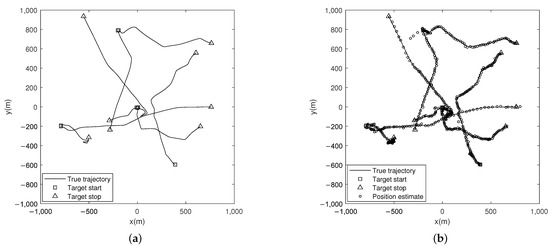
Figure 1. (a) True trajectories of the targets in the scenario with the same heavy-tailed degrees. (b) Position estimates of this simulation.

For the parameters required in the update, we use a maximum number of iterations $N_{max}=10$, a cutoff distance $\sigma =0.1$, and a tuning parameter $\tau =1$. Each target has a probability $p_D=0.98$ of being detected by the sensor. The maximum number of global hypotheses is set to $N_{hypo}=200$. The pruning weight thresholds of the Poisson and MBM components are set to $w_{Pois}^{\left(T\right)}={10}^{-5}$ and $w_{mbm}^{\left(T\right)}={10}^{-4}$, respectively. The threshold of the ellipsoidal gating is set to $T_g=40$. The Bernoulli components, whose existence probability is lower than $r_B^{\left(T\right)}={10}^{-5}$, are removed.

In this test, to match the scenario of the same heavy-tailed degrees ($p_w=p_v=0.9$), the DOFs of the process and measurement noises are set to $d_w=d_v=4$. Figure 1b shows the position estimates for this simulation. Note that each boundary of the sparse and dense estimation points indicates a severe change in the target velocity.

Figure 2a and Figure 2b, respectively, show the comparisons of the OSPA distances (for $p=1$ and $c=100$) and cardinality estimates of the proposed filter with the STM-LMB, STM-GLMB, and STM-CBMeMBer filters after 100 Monte Carlo runs, indicating better performance compared to the existing filters. It is worth mentioning that the OSPA fluctuation at $t=70$ s in Figure 2a is caused by the gradual decrease in the component’s probability of existence when the target disappears. We also use the GOSPA metric, with parameters $p=2$, $c=30$, and $\alpha =2$, to further evaluate the tracking performance of the proposed filter. The comparisons of the GOSPA error, localization error (LE), missed targets error (ME), and false targets error (FE) are shown in Figure 3. It is evident that the R-ST-PMBM filter exhibits a smaller GOSPA error, LE, and ME most of the time. Note that all the errors are root-squared versions. From Figure 3c, we can conclude that the error at $t=1$ s in Figure 2a is caused by the misestimation of the true targets when the filtering process starts. These errors also exist in the simulation of other PMBM-based filters.

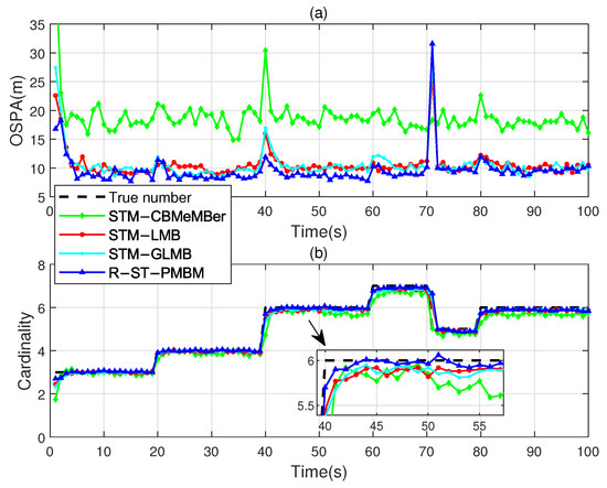
Figure 2. (a) OSPA distances of the four filters versus time. (b) Cardinality estimates versus time.

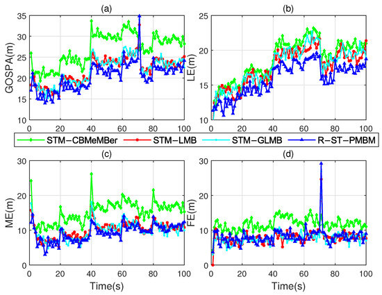
Figure 3. Comparison of the errors among the four filters versus time. (a) GOSPA error. (b) LE. (c) ME. (d) FE.

Table 1 shows the indices of the average OSPA (AOSPA) distance [23], average GOSPA error (AGOSPA), average LE (ALE), average ME (AME), average FE (AFE), and average running time (ART) (in s) of the four filters after 100 Mont Carlo runs. These results demonstrate that our filter exhibits the best tracking performance in the scenario with the same heavy-tailed degrees. It should be noted that compared to the STF-based filters, the performance advantage of the proposed filter is mainly due to the combined effects of the following factors: avoiding the use of moment-matching approximations with large errors, using a Gaussian-based PMBM posterior to approximate the truth posterior, and inheriting the high performance of the standard PMBM filter.

Table 1. Numerical results of the four filters in the scenario with the same heavy-tailed degrees.

Filter	AOSPA	AGOSPA	ALE	AME	AFE	ART
STM-CBMeMBer	18.801	26.967	18.634	15.313	11.78	4.035
STM-LMB	10.598	21.924	17.574	10.136	7.92	8.708
STM-GLMB	10.561	21.934	17.755	9.886	7.771	12.452
R-ST-PMBM	9.571	20.299	15.923	9.25	8.138	4.02

4.2. Scenario with Different Heavy-Tailed Degrees

To evaluate the pertinence of the design of the proposed filter, we consider a scenario in which the process noise and the measurement noise have different heavy-tailed degrees. Before the test, to facilitate the selection of appropriate DOFs, we studied the tracking performance of the proposed filter under different heavy-tailed process and measurement noises with different DOF settings, and the results are shown in Figure 4. For Figure 4a, we set the process noise to null and $d_w=4$, whereas for Figure 4b, we set $p_v=0.9$ and $d_v=4$, and the remaining parameters were unchanged.

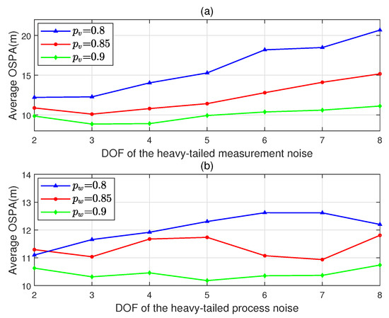
Figure 4. AOSPA versus DOF under noises with different heavy-tailed degrees. (a) Process noise is null, $d_w=4$. (b) $p_v=0.9$, $d_v=4$.

In this test, we change the superposition proportion of the process noise (see Equation (93)) to $p_w=0.8$, which can increase the number of outliers in the mixed process noise and result in a larger heavy-tailed degree compared to the measurement noise. As shown in Figure 4b, the DOF of the process noise is set to $d_w=2$, and the other noise parameters are consistent with the previous test.

Theoretically, to track the targets in this scenario, the one-step predicted PDF and likelihood PDF (see Equations (10) and (11)) are usually required to be set to different DOFs, i.e., $d_w\ne d_v$. But this is impossible in the STM-CBMeMBer, STM-LMB, and STM-GLMB filters. Therefore, for these three filters, we successively set the DOFs to $d_w=d_v=3$ and $d_w=d_v=4$ (due to the existence of moment matching, in the STF-based filters, the DOFs cannot be set to 2). We set the DOFs of the R-ST-PMBM filter to $d_w=2$ and $d_v=4$. Figure 5 and Figure 6 show comparisons of the OSPA distances, cardinality estimates, and GOSPA metrics, respectively.

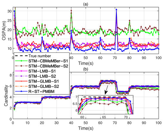
Figure 5. (a) OSPA distances of the four filters with different DOF settings. (b) Cardinality estimates versus time.

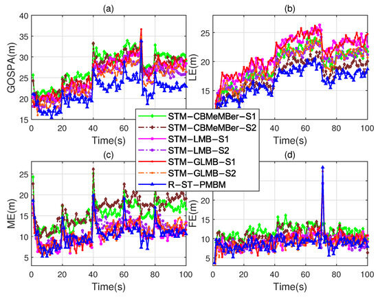
Figure 6. Comparison of the errors among the four filters with different DOF settings. (a) GOSPA error. (b) LE. (c) ME. (d) FE.

Note that the extensions “S1” and “S2” in the legends in Figure 5 and Figure 6 represent the DOF settings $d_w=d_v=3$ and $d_w=d_v=4$, respectively. It is evident that the OSPA distance and the GOSPA error of the R-ST-PMBM filter are lower compared to the existing filters, except for the fluctuation when the target number is reduced (at $t=70$ s). Table 2 provides a comparison of the different indices, where we can see that the overall performance of the R-ST-PMBM filter is better compared to the existing filters. Compared to the previous test, the performance advantage of the R-ST-PMBM filter in the scenario of noises with different heavy-tailed degrees is enhanced. It should be pointed out that the operational efficiency advantage of the proposed filter stems from its linear computational complexity in the number of hypotheses, whereas the complexity of the STM-LMB and STM-GLMB filters is quadratic.

Table 2. Numerical results of the four filters in the scenario with different heavy-tailed degrees.

Filter	DOF Settings	AOSPA	AGOSPA	ALE	AME	AFE	ART
STM-CBMeMBer	$d_w=d_v=3$	19.203	27.541	19.402	15.342	11.785	4.125
	$d_w=d_v=4$	19.387	26.393	17.524	16.511	10.484	3.739
STM-LMB	$d_w=d_v=3$	11.909	25.567	21.198	10.487	9.31	9.141
	$d_w=d_v=4$	12.306	24.412	19.276	11.723	8.96	8.688
STM-GLMB	$d_w=d_v=3$	12.101	25.864	21.354	10.609	9.616	14.978
	$d_w=d_v=4$	11.936	24.122	19.246	11.183	8.895	12.666
R-ST-PMBM	$d_w=2$, $d_v=4$	10.379	21.624	16.499	10.43	8.839	4.516

4.3. Real Data Scenario

The effectiveness of the R-ST-PMBM filter is also verified in a real data scenario. Essentially, all the target maneuvers and sensor measurement outliers can be considered as the affected results of the heavy-tailed process and measurement noises, respectively. The larger the heavy-tailed degree of the noise, the more severe the target motion or the sensor measurement outliers, and vice versa. In this simulation, the surveillance area is restricted to [8000, 11,000] × [1000, 7000] (in m), and the real data are obtained from radar measurements of two aircraft in the surveillance area. The target motions and sensor measurements are projected onto a two-dimensional plane. Two targets appeared successively in this area, lasting 64 s, and were detected 48 times by the sensor.

The scanning interval T (see Equation (91)) of the sensor is not constant. The newborn parameters are set to $w_{\gamma ,k}=1$, $m_{\gamma ,k}={[8727,0,1399,0]}^T$, and $P_{\gamma ,k}=\mathrm{diag}\left(\right[50,50,50,50]{)}^2$. The nominal standard deviations of the process and measurement noises are set to ${\sigma }_w=30$ m/s² and ${\sigma }_v=10$ m, and the DOFs are set to $d_w=d_v=4$. The parameters not mentioned can be referred to in Section 4.1. Figure 7 shows the true trajectories and position estimates. Figure 8 shows the OSPA distance and cardinality estimate comparisons of the four filters. It can be seen that the R-ST-PMBM filter has the best tracking effect among these filters. The comparison results of the GOSPA metrics, shown in Figure 9, also support this conclusion. Note that the large fluctuation of the proposed filter at time step $k=18$ is directly caused by the sudden increase in the radar scanning period.

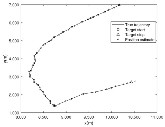
Figure 7. True trajectories and position estimates in the real data scenario.

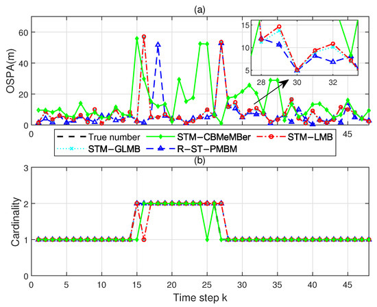
Figure 8. (a) OSPA distances of the four filters in the real data scenario. (b) Cardinality estimates versus time.

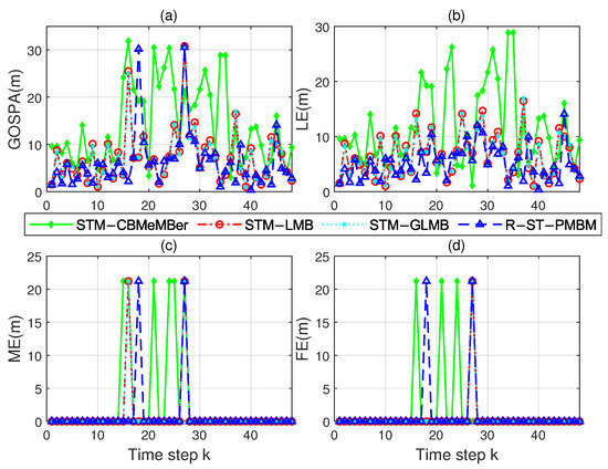
Figure 9. Comparison of the errors among the four filters in the real data simulation. (a) GOSPA error. (b) LE. (c) ME. (d) FE.

The numerical results of the four filters are provided in Table 3. It can be seen that, compared to the other filters, the R-ST-PMBM filter demonstrates a significant overall performance advantage in this real data scenario.

Table 3. Numerical results of the four filters in the real data simulation.

Filter	AOSPA	AGOSPA	ALE	AME	AFE	ART
STM-CBMeMBer	14.555	14.111	11.581	2.652	1.326	0.302
STM-LMB	7.964	7.353	6.62	0.884	0.442	1.152
STM-GLMB	7.977	7.366	6.634	0.884	0.442	1.531
R-ST-PMBM	6.623	6.18	5.103	0.884	0.884	0.416

5. Conclusions

In this paper, an improved PMBM filter, called the R-ST-PMBM filter, was proposed to better perform MTT under heavy-tailed process and measurement noises, which provided a Student’s t-based Gaussian approximation to the components of the PMBM density. The one-step prediction and measurement likelihood were modeled as Student’s t-distributions with different DOFs, enabling our filter to be more adaptable to real environments. The scale matrix of the one-step predicted PDF was assumed to be unknown and modeled as an IW distribution, increasing the filter’s robustness. The resulting Student’s t-based hierarchical Gaussian state-space model was iterated to derive a posterior PDF by introducing the auxiliary variables and the VB approach and then approximated to Gaussian to obtain a closed-form recursion in the update step. The simulation results show that in the heavy-tailed process and measurement noise environment, the R-ST-PMBM filter achieves better overall performance compared to the existing filters, even under these noises with different heavy-tailed degrees.

In our future work, maneuvering target tracking in a real-world environment will become an application field for the proposed filter. Applying this filter to extended target tracking is also a possible research topic.

References

- Vo, B.T.; Ma, W.K. The Gaussian mixture probability hypothesis density filter. IEEE Trans. Signal Process. 2006, 54, 4091–4104. [Google Scholar] [CrossRef]
- Dong, P.; Jing, Z.; Leung, H.; Wang, J. Student-t mixture labeled multi-Bernoulli filter for multi-target tracking with heavy-tailed noise. Signal Process. 2018, 152, 331–339. [Google Scholar] [CrossRef]
- Lian, Y.; Lian, F.; Hou, L. Robust labeled multi-Bernoulli filter with inaccurate noise covariances. In Proceedings of the 25th International Conference on Information Fusion, Linköping, Sweden, 4–7 July 2022. [Google Scholar]
- Wang, X.; Xie, W.; Li, L. Labeled Multi-Bernoulli Maneuvering Target Tracking Algorithm via TSK Iterative Regression Model. Chinese J. Electron. 2022, 31, 227–239. [Google Scholar]
- Yang, Z.; Li, X.; Yao, X.; Sun, J.; Shan, T. Gaussian process Gaussian mixture PHD filter for 3D multiple extended target tracking. Remote Sens. 2023, 15, 3224. [Google Scholar] [CrossRef]
- Mahler, R. Statistical Multisource-Multitarget Information Fusion; Artech House, Inc.: Norwood, MA, USA, 2007. [Google Scholar]
- Vo, B.T.; Vo, B.N.; Cantoni, A. The cardinality balanced multi-target multi-Bernoulli filter and its implementations. IEEE Trans. Signal Process. 2009, 57, 409–423. [Google Scholar]
- Vo, B.N.; Vo, B.T.; Hoang, H.G. An efficient implementation of the generalized labeled multi-Bernoulli filter. IEEE Trans. Signal Process. 2017, 65, 1975–1987. [Google Scholar] [CrossRef]
- Reuter, S.; Vo, B.T.; Vo, B.N.; Dietmayer, K. The labeled multi-Bernoulli filter. IEEE Trans. Signal Process. 2014, 62, 3246–3260. [Google Scholar]
- Williams, J.L. Marginal multi-Bernoulli filters: RFS derivation of MHT, JIPDA, and association-based MeMBer. IEEE Trans. Aerosp. Electron. Syst. 2015, 51, 1664–1687. [Google Scholar] [CrossRef]
- García-Fernández, A.F.; Williams, J.L.; Granstöm, K. Poisson multi-Bernoulli mixture filter: Direct derivation and implementation. IEEE Trans. Aerosp. Electron. Syst. 2018, 54, 1883–1901. [Google Scholar] [CrossRef]
- Xia, Y.; Granström, K.; Svensson, L.; García-Fernández, A.F. Performance evaluation of multi-Bernoulli conjugate priors for multi-target filtering. In Proceedings of the 20th International Conference on Information Fusion, Xi’an, China, 10–13 July 2017. [Google Scholar]
- Du, H.; Xie, W. Extended target marginal distribution Poisson multi-Bernoulli mixture filter. Sensors 2020, 20, 5387. [Google Scholar] [CrossRef]
- García-Fernández, A.F.; Svensson, L.; Williams, J.L.; Xia, Y.; Granstöm, K. Trajectory Poisson multi-Bernoulli filters. IEEE Trans. Signal Process. 2020, 68, 4933–4945. [Google Scholar] [CrossRef]
- Li, Y.; Wei, P.; You, M.; Wei, Y.; Zhang, H. Joint detection, tracking, and classification of multiple extended objects based on the JDTC-PMBM-GGIW filter. Remote Sens. 2023, 15, 887. [Google Scholar] [CrossRef]
- Li, G.; Kong, L.; Yi, W.; Li, X. Multiple model Poisson multi-Bernoulli mixture filter for maneuvering targets. IEEE Sens. J. 2021, 21, 3143–3154. [Google Scholar] [CrossRef]
- Li, W.; Gu, H.; Su, W. Robust Poisson multi-Bernoulli mixture filter with inaccurate process and measurement noise covariances. IEEE Access 2020, 8, 52209–52220. [Google Scholar] [CrossRef]
- Qiu, H.; Huang, G.; Gao, J. Variational Bayesian labeled multi-Bernoulli filter with unknown sensor noise statistics. Chin. J. Aeronaut. 2016, 29, 1378–1384. [Google Scholar]
- Li, G.; Wei, P.; Li, Y.; Gao, L.; Zhang, H. A robust fast LMB filter for superpositional sensors. Signal Process. 2020, 174, 107606. [Google Scholar] [CrossRef]
- Ting, J.A.; Theodorou, E.; Schaal, E. Learning an outlier-robust Kalman filter. In Proceedings of the 18th European Conference on Machine Learning, Warsaw, Poland, 17–21 September 2007; pp. 748–756. [Google Scholar]
- Zhu, H.; Leung, H.; He, Z. A variational Bayesian approach to robust sensor fusion based on Student-t distribution. Inf. Sci. 2013, 221, 201–214. [Google Scholar] [CrossRef]
- Li, W.; Jia, Y.; Du, J.; Zhang, J. PHD filter for multi-target tracking with glint noise. Signal Process. 2014, 94, 48–56. [Google Scholar] [CrossRef]
- Liu, Z.; Huang, B.; Zou, Y.; Li, L. Multi-object Bayesian filter for jump Markov system under glint noise. Signal Process. 2019, 157, 131–140. [Google Scholar] [CrossRef]
- Dong, P.; Leung, H.; Jing, Z.; Shen, K.; Li, M. The labeled multi-Bernoulli filter for multitarget tracking with glint noise. IEEE Trans. Aerosp. Electron. Syst. 2019, 55, 2253–2268. [Google Scholar] [CrossRef]
- Hou, L.; Lian, F.; Tan, S.; Xu, C.; De Abreu, G.T.F. Robust generalized labeled multi-Bernoulli filter for multitarget tracking with unknown non-stationary heavy-tailed measurement noise. IEEE Access 2021, 9, 94438–94453. [Google Scholar] [CrossRef]
- Roth, M.; Özkan, E.; Gustafsson, F. A Student’s t filter for heavy-tailed process and measurement noise. In Proceedings of the 2013 IEEE Conference on Acoustics, Speech and Signal Processing, Vancouver, BC, Canada, 26–31 May 2013. [Google Scholar]
- Wang, M.; Ji, H.; Zhang, Y.; Hu, X. A Student’s t mixture cardinality-balanced multi-target multi-Bernoulli filter with heavy-tailed process and measurement noises. IEEE Access 2018, 6, 51098–51109. [Google Scholar] [CrossRef]
- Hu, X.; Zhang, Q.; Song, B.; Zhao, M.; Xia, Z. Student-t mixture GLMB filter with heavy-tailed noises. In Proceedings of the 2013 IEEE Conference on Signal Processing, Communications and Computing, Xi’an, China, 25–27 October 2022. [Google Scholar]
- Huang, Y.; Zhang, Y.; Li, N.; Wu, Z. A novel robust Student’s t-based Kalman filter. IEEE Trans. Aerosp. Electron. Syst. 2017, 53, 1545–1554. [Google Scholar] [CrossRef]
- Huang, Y.; Zhang, Y.; Li, N.; Wu, Z. A robust Gaussian approximate fixed-interval smoother for nonlinear systems with heavy-tailed process and measurement noises. IEEE Signal Proc. Let. 2016, 23, 468–472. [Google Scholar] [CrossRef]
- O’Hagan, A.; Forster, J. Kendall’s Advanced Theory of Statistics, Vol 2B: Bayesian Inference; Arnold Publishers: London, UK, 2004; pp. 402–406. [Google Scholar]
- Bishop, C. Pattern Recognition and Machine Learning (Information Science and Statistics); Springer: New York, NY, USA, 2006; pp. 462–466. [Google Scholar]
- Schihmacher, D.; Vo, B.T.; Vo, B.N. A consistent metric for performance evaluation of multi-object filters. IEEE Trans. Signal Process. 2008, 56, 3447–3457. [Google Scholar] [CrossRef]
- Rahmathullah, A.S.; García-Fernández, A.F.; Svensson, L. Generalized optimal sub-pattern assignment metric. In Proceedings of the 20th International Conference on Information Fusion, Xi’an, China, 10–13 July 2017. [Google Scholar]
- Huang, Y. Researches on High-Accuracy State Estimation Methods and Their Applications to Target Tracking and Cooperative Localization. Ph.D. Dissertation, Harbin Engineering University, Harbin, China, 2018; pp. 162–163. [Google Scholar]
Disclaimer/Publisher’s Note: The statements, opinions and data contained in all publications are solely those of the individual author(s) and contributor(s) and not of MDPI and/or the editor(s). MDPI and/or the editor(s) disclaim responsibility for any injury to people or property resulting from any ideas, methods, instructions or products referred to in the content. |
© 2023 by the authors. Licensee MDPI, Basel, Switzerland. This article is an open access article distributed under the terms and conditions of the Creative Commons Attribution (CC BY) license (https://creativecommons.org/licenses/by/4.0/).