Article

Spectral Segmentation Multi-Scale Feature Extraction Residual Networks for Hyperspectral Image Classification

1
School of Computer Science, China University of Geosciences, Wuhan 430078, China
2
Hubei Key Laboratory of Intelligent Geo-Information Processing, China University of Geosciences, Wuhan 430078, China
*
Author to whom correspondence should be addressed.
Remote Sens. 2023, 15(17), 4219; https://doi.org/10.3390/rs15174219
Submission received: 2 July 2023 / Revised: 18 August 2023 / Accepted: 26 August 2023 / Published: 28 August 2023

Abstract

:
Hyperspectral image (HSI) classification is a vital task in hyperspectral image processing and applications. Convolutional neural networks (CNN) are becoming an effective approach for categorizing hyperspectral remote sensing images as deep learning technology advances. However, traditional CNN usually uses a fixed kernel size, which limits the model’s capacity to acquire new features and affects the classification accuracy. Based on this, we developed a spectral segmentation-based multi-scale spatial feature extraction residual network (MFERN) for hyperspectral image classification. MFERN divides the input data into many non-overlapping sub-bands by spectral bands, extracts features in parallel using the multi-scale spatial feature extraction module MSFE, and adds global branches on top of this to obtain global information of the full spectral band of the image. Finally, the extracted features are fused and sent into the classifier. Our MSFE module has multiple branches with increasing ranges of the receptive field (RF), enabling multi-scale spatial information extraction at both fine- and coarse-grained levels. On the Indian Pines (IP), Salinas (SA), and Pavia University (PU) HSI datasets, we conducted extensive experiments. The experimental results show that our model has the best performance and robustness, and our proposed MFERN significantly outperforms other models in terms of classification accuracy, even with a small amount of training data.

1. Introduction

Hyperspectral images (HSI), typically with several hundred contiguous spectral bands per pixel, include an abundance of spectral and spatial information and have very high spatial resolution and correlation [1]. HSI is currently employed in numerous applications, including defense [2], land cover analysis [3], crop monitoring [4], and medical disease diagnosis [5]. One of the most important tasks in HSI analysis is hyperspectral image classification (HSIC), which involves assigning each pixel in an HSI to a specific land cover class using spatial and spectral information.
Early HSIC research focused on the use of traditional machine learning methods, such as support vector machines (SVM) [6], k-nearest neighbors [7], and logistic regression [8], among others. At the same time, considering the existence of redundant information and noise in the spectral bands, as well as the small number of training samples in HSIC compared to the high dimensionality of the HSI data, which can easily be prone to overfitting and Hughes phenomenon [9], therefore, approaches to dimensionality reduction, such as principal component analysis (PCA) [10], subspace learning [11], and sparse representation [12] has been widely used to solve these problems. Nevertheless, these approaches can only extract superficial characteristics of the image based on the spectral information of HSI, ignoring the spatial information and cannot fully extract the image’s deeper features.
To further improve the performance of HSIC by exploiting spatial information, Zhong et al. [13] presented an iterative approach to obtain spatial information from spectral classification data samples using selective spatial filters. Duan et al. [14] used local edge-preserving filtering and global edge-preserving smoothing to obtain edge-preserving features and used the superpixel segmentation method and support vector machine to obtain hyperspectral image classification results. Zhang et al. [15] presented a model based on the local correntropy matrix (LCEM), which reduces the dimensionality of the original hyperspectral data, selects local neighbors in a sliding window using cosine distance to construct LCEM, and finally sends the correntropy matrices to the support vector machine for classification. Additionally, extended multi-attribute profile methods (EMAP) [16], Markov random field-based methods [17] and superpixel segmentation-based methods [18] are additional typical methods for the spatial classification of spectral.
In recent years, a growing number of deep learning approaches have been applied to HSIC, such as stacked autoencoders (SAE) [19], convolutional neural networks (CNNs) [20,21], and recurrent neural networks (RNNs) [22], among others. Among them, CNN is widely used due to its advantages of automatic extraction of image features and self-learning updates of parameters. Liu et al. [23] presented a 2D-CNN capable of automatically learning features from complex hyperspectral image data structures for HSIC. Yu et al. [24] suggested a lightweight 2D-3D CNN model to efficiently extract fine features. Chen et al. [20] presented a 3D-CNN model combined with regularized depth feature extraction. Roy et al. [25] presented a hybrid spectral CNN made up of 2D and 3D-CNN. These 3D-CNN classification frameworks have good classification performance but also require high computational costs. Since 2D-CNN operates on a two-dimensional space without considering the image depth, and is much less in terms of the number of parameters compared to 3D-CNN, we have used 2D-CNN to extract spatial and spectral features in order to be able to reduce the computational complexity of our model.
The depth of the network affects the majority of models’ performance, yet numerous studies have demonstrated that as network depth rises, CNN models suffer from information loss due to the gradient disappearance problem [26], resulting in poor results. The proposal of ResNet [27] and DenseNet [28] effectively addressed this problem, and subsequently, many scholars have added them to deep network models in conjunction with CNN for HSIC. Paoletti et al. [29] presented a ResNet model (PResNet) based on a pyramidal bottleneck residual cell ground that can perform fast and accurate HSIC combining spatial and spectral information. Li et al. [30] presented a double branch and double attention mechanism network (DBDA) with a dense connection structure and Mish activation function. The model’s performance in terms of optimization and generalization was also enhanced. Wu et al. [31] presented a reparameterization-based null-spectrum residual network (RepSSRN) and used it for HSIC. The residual network has a powerful feature transformation capability, so we continued to use the residual structure and dense blocks in the proposed model.
Although the receptive field (RF) is the area that directly influences the convolution operation, the majority of the current CNN models for HSIC employ a fixed-size RF for feature extraction, which limits the model learning weights. Typically, larger RFs are unable to capture fine-grained structures, but coarse-grained image structures are typically eliminated by RFs that are too tiny [32]. Therefore, to synthetically extract multi-scale information at both the fine-grained and coarse-grained levels of an image, we developed a spectral segmentation-based multi-scale spatial feature extraction residual network (MFERN) for HSIC. Specifically, we first proposed a multi-scale spatial feature extraction module, MSFE, which separates the input image’s spectral bands into various RFs for each branch. We stack convolutional layers with a 3 × 3 kernel size to increase the RF while decreasing the computational cost. Moreover, we apply “selective kernel” (SK) convolution [33] operations to all but the first two branches to improve the model’s effectiveness and adaptability. In addition, we suggest an improved spectral segmentation residual module SSRM, which divides the input patches into a number of equal-width groups along the spectral dimension, constructs multiple parallel convolutional networks to extract spatial and spectral features, and finally fuses the features of each parallel CNN. It should be noted that considering the simplicity of the practice, we do not really build many CNNs but use grouped convolution for equivalent implementation. We replace the normal convolution layer with grouped convolution [34] based on the dense block in the DenseNet network [28] and combine MSFE with grouped convolution to replace the 3 × 3 kernel size convolution layers in the dense block. Additionally, considering that the parallel CNN constructed by grouping operations extracts features from certain spectral bands independently, we add a global branch consisting of a normal 1 × 1 kernel size convolutional layer and an MSFE module to the original residual structure to extract the feature map’s global information. In conclusion, the following are this paper’s significant contributions:
(1)
A multi-scale spatial feature extraction module MSFE is proposed, which extracts information at different scales using convolutional layers with different receptive field sizes after dividing the spectral bands, exploiting the multi-scale potential at a finer granularity level for efficient and comprehensive extraction of spatial information.
(2)
In this paper, we propose an improved spectral segmentation residual module SSRM, which combines the MSFE module with grouped convolution, divides the input patches along the spectral dimensions, constructs multiple parallel CNNs to extract the features separately and adds a global branch on top of the original residual structure to synthesize the local and global information of the space and spectrum.
(3)
The effectiveness of the presented module was tested using three HSI datasets, and the presented MFERN approach used fewer training samples to reach state-of-the-art classification accuracy.
The remainder of the paper is structured as follows. The second part details the specifics of the MFERN method’s implementation details, the third part delivers the results and analysis of the experiments, the fourth part is a discussion of the strengths and weaknesses of the methodology of this paper, and the fifth provides part a summary of the paper’s work and recommendations for further study.

2. Materials and Methods

We initially describe the proposed multi-scale spatial feature extraction module MSFE in this section, followed by a modified spectral segmentation residual module (SSRM) for the combined acquisition of global and local information of space and spectrum, and finally summarize the general framework of our proposed multi-scale spatial feature extraction residual network (MFERN) approach based on spectral segmentation.

2.1. Multi-Scale Spatial Feature Extraction Module

Let the HSI dataset be X R H × W × B , where B stands for the number of spectral bands, H and W stand for the height and width of the spatial dimension, respectively. The input X p R p × p × B to MFERN is a patch of size p × p × B , with p being the size of the patch given in advance. Generally speaking, the larger the size p of a patch, the more spatial information it contains, so it is particularly crucial to understand how to extract spatial information more effectively and thoroughly, for which we present the Multi-Scale Spatial Feature Extraction module (MSFE). Figure 1 depicts the basic construction of this module.
Specifically, for a feature map input, x R p × p × c , we partition it uniformly into s subsets of feature maps x i , i = 1 , 2 , , s , where each x i has the same spatial size but the number of channels is c / s . Except for x 1 , which does not go through the convolution layer and is a shortcut connection, the remaining x i , i = 2 , 3 , , s of the corresponding convolutional layers have increasing RF in that order. As Szegedy et al. [35] suggest that convolution with larger spatial filters is computationally extraordinarily expensive, yet reducing its size comes at a significant cost in terms of expressivity. As shown in Figure 2, where Figure 2a indicates that the feature map size of a 5 × 5-sized feature map after one layer of 5 × 5 convolution is 1 × 1, and Figure 2b indicates that the feature map size of a 5 × 5-sized feature map after two layers of 3 × 3 convolution is also 1 × 1, which suggests that the two layers of 3 × 3 convolution have the same RF as one layer of 5 × 5 convolution, and thus the 5 × 5 convolution can be replaced by two layers of 3 × 3 convolution. Thus, we acquire a larger size convolution and RF equivalently by repeatedly stacking smaller 3 × 3 convolutions, with enhanced non-linearity due to the use of one more activation function for two convolution layers compared to one. Specifically, x 2 passes through only one 3 × 3 convolutional layer, while x i , i = 3 , 4 , , s first passes through i 2 3 × 3 convolutional layers, respectively, denoted by K j ( · ) , j = 1 , 2 , , i 2 , and K j ( · ) consists of convolution, Batch Normalization (BN) [36] and ReLU [37] activation functions (ReLU) in turn, followed by feature cascading, where the space size of the cascaded feature map x c o n c a t remains unchanged and the number of channels becomes s 2 times the original one.
x c o n c a t = K 1 ( x 3 ) K 2 ( K 1 ( x 4 ) ) K j ( K ( K 1 ( x i ) ) ) s 3 , i = 3 , 4 , , s , j = 1 , 2 , , i 2
where ⊕ denotes the feature concat operation for the channel dimension. Note that all feature maps are subjected to a fill operation to maintain the feature map’s original spatial size.
The cascaded feature map x c o n c a t is subjected to a Selective Kernel (SK) convolution operation in order to improve the MSFE module’s adaptability, as depicted in Figure 3. Three steps make up this operation: Split, Fuse, and Select. Several pathways with various convolutional kernel sizes are produced by the operation Split. In this paper, the number of paths is s 2 , and the convolutional RF of each path is the same as the convolutional RF of the feature map subset x i , i = 3 , 4 , , s . Therefore, we also use the stacked 3 × 3 convolution to achieve the effect of increasing the convolutional kernel size. The Fuse operation aggregates and combines data from many paths to produce a global and composite representation of the selection weights. The Select operation aggregates feature maps with different kernel sizes based on selection weights. Using the example of s = 4 , i.e., two paths for the SK convolution operation, we will describe in detail the procedure for this operation.
Split: For a given feature map x c o n c a t R p × p × D , where D = c 2 c s , two transformations F 3 × 3 : x c o n c a t U 3 R p × p × D and F 5 × 5 : x c o n c a t U 5 R p × p × D are first performed, with kernel sizes of 3 and 5, respectively; where both F 3 × 3 and F 5 × 5 are the same as previous operations, consisting of the convolution, BN and ReLU in turn, and the convolution of the 5 × 5 kernel is equivalently formed by stacking the convolutions of two 3 × 3 kernels.
Fuse: One basic idea for implementing adaptive tuning of neurons with different sizes of RF is to design a gate mechanism for controlling the information flow into the following layer of neurons from many branches carrying information at varied scales. The result of fusing multiple (in this case is two) pathways by summing the elements is first:
U = U 3 + U 5
Global average pooling [38] is then used to generate channel-wide statistics for G R D to embed the global information.
G d = F g a p ( U d ) = 1 p × p m = 1 p n = 1 p U d ( m , n )
where G d is the dth element of G and F g a p stands for global average pooling.
Finally, to facilitate guidance on precise and adaptable selection, a compact feature Z R l × 1 is produced by a fully connected layer of:
Z = F f c ( G ) = δ ( F B N ( W G ) )
where the ReLU activation function is δ , F B N stands for batch normalization and W R l × D . A reduction rate r is used to adjust the value of l to evaluate its impact on the model’s effectiveness:
l = m a x ( D r , L )
where L stands for the minimum value of l. In this paper, L = 32 is set.
Select: Use cross-channel soft attention, guided by the compact feature descriptor Z, to adaptively select information at different spatial scales. Specifically, a softmax operator is applied to the numbers on the channel:
a m = e A m Z e A m Z + e B m Z , b m = e B m Z e A m Z + e B m Z
where A and B R D × l , the soft attention vectors of U 3 and U 5 are denoted by a and b, respectively. Notably, A m R 1 × l is the mth row of A and a m is the mth element of a, as are B m and b m . The attention weights on each kernel are used to create the final feature map x c o n c a t , which is calculated as follows:
x c o n c a t m = a m · U 3 m + b m · U 5 m , a m + b m = 1
where x c o n c a t = [ x c o n c a t 1 , x c o n c a t 2 , , x c o n c a t m ] , x c o n c a t m R p × p , · denotes the multiplication operation. For the resulting final feature map x c o n c a t , some of the channels have RFs of size 5 × 5, some have RFs of size 7 × 7, and the rest have RFs of size 11 × 11, so x c o n c a t has rich multi-scale spatial features and gains both the advantage of multiple channels and a priori knowledge of inter-channel attention. Note that the formulae provided above are for the case where s = 4. Cases with more paths can be deduced by extending Equations (1), (2), (6) and (7).
Finally, after cascading all subsets of feature maps and putting them through the ReLU activation function, the MSFE module’s final output y is obtained:
y = δ ( x 1 + x 2 + x c o n c a t )
where δ is the ReLU activation function.

2.2. Spectral Segmentation Residual Module

Our SSRM module divides the input patches into a number of equal-width groups and constructs multiple parallel CNNs to extract spatial and spectral features from different group subbands, but in practice, we do not actually construct these parallel CNNs but rather use packet convolution for equivalent implementation. In addition, we further improve the residual block by adding a global branch for information fusion at the feature level, which combines the advantages of local and global features to obtain a richer and more comprehensive feature representation. The group convolution equivalence and residual block improvement are discussed in detail below.
Figure 4a shows the basic module designed in DenseNet [28]. Since Xie et al. [34] suggested that grouped convolution has a better FLOPs/accuracy trade-off than ordinary convolution, its ability to improve accuracy while reducing complexity. Let C 0 be the number of input channels, k be the size of the convolution kernel, H × W be the size of the output feature maps, C 1 be the size of the output channels, and the number of groupings is g. Then for normal convolution, its parameter number is K 2 × C 0 × C 1 ; and for grouped convolution, its parameter number is K 2 × C 0 g × C 1 g = K 2 × C 0 × C 1 g , which shows that the total number of parameters of grouped convolution is 1 / g of the number of parameters of ordinary convolution. Thus, we use grouped convolution to replace the original ordinary convolution in (a). In the original module, information from the feature maps is extracted using convolution kernels of kernel size 3 × 3, but it is difficult to extract information at different scales using fixed-size convolution kernels, so we combine the MSFE module introduced in Section 3.1 with grouped convolution, as depicted in Figure 4b, and Figure 4c is an equivalent implementation of (b). Specifically, for an input feature map X i n R p × p × K , we divide it into T feature map subsets by spectral dimension, and the number of spectral bands in each feature map subset b = K / T . If K is not divisible by T, we repeatedly copy the final value of the spectral band to extend the spectral band until it is divisible by K. This leads to:
X i n = { X i n 0 , b , X i n b , 2 b , , X i n ( T 1 ) b , K }
After the spectral division is completed, T sets of parallel feature extraction branches are constructed, and for each set of branches, they first pass through a 1 × 1 kernel size convolutional layer, enabling the combination of information across channels and the addition of non-linear features. This is followed by an MSFE module to extract multi-scale spatial features:
X o u t m = Φ M S F E m ( Φ c o n v 1 m ( X i n ( m 1 ) b , m b ) ) , m = 1 , 2 , , T
where the vector X o u t m is the output of the mth group of branches, Φ M S F E ( · ) denotes the MSFE module, and Φ c o n v 1 ( · ) denotes the convolution layer with a 1 × 1 kernel size.
Finally, we stitch the T features extracted from T sets of parallel branches and after the ReLU we obtain the final output of the module:
X o u t = [ X o u t 1 , X o u t 2 , , X o u t T ]
Considering that the parallel CNN constructed by grouping operations extracts features from certain spectral bands independently and lacks global feature information for the whole spectral band, we added a global branch to the original residual block, which also consists of a 1 × 1 kernel size convolutional layer and an MSFE module, except that instead of grouped convolution, two normal convolutional layers are used. The original branch is used to extract the spatial and spectral features from the local band, while the new global branch is used to extract the global spatial and spectral features from the entire input band. The structure of our designed SSRM is shown in Figure 5.

2.3. Overview of a MFERN

The final complete architecture of the Multi-Scale Spatial Feature Extraction Residual Network (MFERN) based on spectral segmentation is depicted in Figure 6, where the specific parameters of each of these layers are shown in Table 1. The input size for MFERN is p × p × B , where B is the number of spectral bands and p is the patch size. The input bands are split into T groups by the first grouped convolutional layer, then two spectral segmentation residual modules SSRM is connected to extract spectral and spatial features, followed by a general convolutional layer (1 × 1) for fusing spectral features and a global average pooling layer (GAP) for fusing spatial features and reducing the spatial size of the input patch’s spatial size to 1 × 1 . The final classification result is then obtained through the use of softmax regression. The output of the classifier is the conditional probability of the output of class q; it can be utilized to obtain the final result. Suppose the conditional probability is y ^ = [ y ^ 1 , y ^ 2 , , y ^ q ] , then:
y ^ j = e x p ( θ 1 ( j ) T + θ 2 ( j ) ) i = 1 q e x p ( θ 1 ( j ) T + θ 2 ( j ) ) , j = 1 , 2 , , q
where T is the input to the classifier and both θ 1 and θ 2 are parameters. We employ the commonly used minimized cross-entropy loss function to train the framework:
L o s s = i = 1 n j = 1 q y j ( i ) l o g y ^ j i
where the truth and prediction labels are y and y ^ , respectively, n is the total amount of minimum batch samples, and the total amount of categories is q.

3. Results

3.1. Dataset

In this section, we design experiments to assess how well our suggested model performs on three commonly used datasets: Indian Pines, Salinas, and Pavia University.
Indian Pines (IP) dataset was collected over the Indian Pines Test Site in northwest Indiana by the 224-band Airborne Visible/Infrared Imaging Spectrometer (AVIRIS) [39], covering 224 spectral bands between 0.4 and 2.5 um in wavelength. The image size was 145 × 145 and contained 16 vegetation classes. Twenty-four water absorption bands were removed, leaving 200 bands available for training.
Salinas (SA) dataset, which spans 224 spectral bands with wavelengths ranging from 0.4 to 2.5 um, was collected by AVIRIS over the Salinas Valley in California. The image size is 512 × 217 and contains 16 land cover classes. Twenty water absorption bands were removed from the experiment, and the actual bands used for training were 204.
Pavia University (PU) dataset was acquired over Pavia, northern Italy, by the Reflection Optical System Imaging Spectrometer (ROSIS) [40] and covers 103 spectral bands between 0.38 and 0.86 um in wavelength. The image size is 610 × 340 and contains nine land cover classes.
We pre-processed the data by first normalizing the values to the range [0, 1], followed by a data augmentation operation that flipped the input patch vertically or horizontally and then randomly rotated it by 90 , 180 or 270 .
For the IP dataset, we used 5% of the labeled samples for training, 5% for validation, and 90% for testing. On the other hand, for the SA and PU datasets, we used 0.5% of the labeled samples for training, 0.5% for validation, and 99% for testing. The number of training, validation, and testing samples for each class is displayed in Table 2, Table 3 and Table 4. We selected the best model on the validation set to be evaluated on the testing set, and we divided the labeled samples 10 times at random, with all results being the average of these 10 runs.

3.2. Experimental Setup

To assess the performance of the MFERN model, we conducted experiments on an Intel(R) Core(TM) i7-9700K CPU @ 3.60 GHz and an NVIDIA GeForce RTX 2080 using the Pytorch framework. We used the Adam [41] optimizer to update all training parameters in the framework.
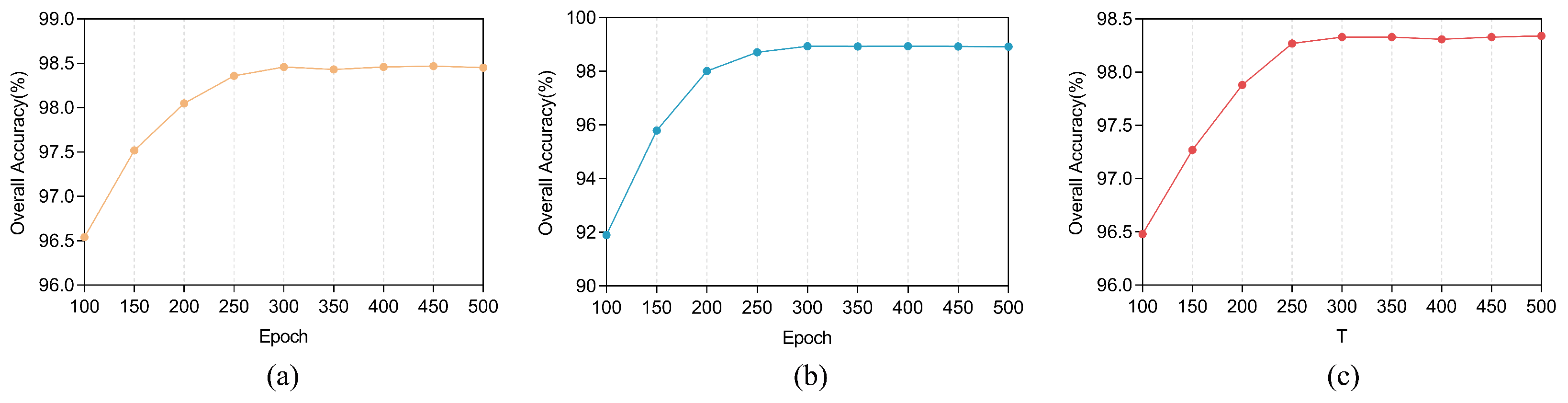
Training epochs have a direct impact on the model. Fewer training rounds may not be enough for the model to fully learn the complex patterns of the data, while more training epochs may cause the model to overfit the training data. Additionally, as the training epochs increase, the model training time also increases. Therefore, in order to find a suitable training epochs setting that avoids overfitting and underfitting while making the training time as small as possible, we conducted experimental exploration. Specifically, we initially set the maximum training epoch = 500 when training on each dataset and output the OA value of the model on the validation set when epoch = { 100 , 150 , 200 , 250 , 300 , 350 , 400 , 450 , 500 } during the training process, and then finally plot a graph to observe the change of OA value with the increase in epochs, the experimental results are shown in Figure 7, and it can be observed that on the three datasets when the epoch is less than 250, the model has poor accuracy and exhibits the characteristics of underfitting. This is because the model has not yet sufficiently learned the complex patterns of the input data to capture the underlying relationships of the data. At this point, the model’s fitting ability is weak and cannot match the training data well. As the training epochs increase, the model gradually improves its fitting ability and reduces underfitting to some extent. When epoch = 300, the model converges, and the model accuracy changes weakly when the epochs increase again after that; therefore, in order not to increase the training time of the model, all the experiments after that are trained with 300 epochs.
The batch size is set to 128, the initial learning rate (lr) is set to 0.001, and the network was trained from scratch without using predefined weights. At 100 epochs, the lr is multiplied by a factor of 0.1, changing to 0.0001, and at 250 epochs, the lr continues to be multiplied by a factor of 0.1, changing to 0.00001. The precision (OA), average precision (AA), and Kappa coefficient act as evaluation metrics to assess the effectiveness of the suggested approach.

3.3. Effect of Input Patch Size

The size of the input patch determines how much spatial information it contains. In general, the larger the input patch, the more local spatial information it contains, but at the same time, the more interfering pixels it contains, or it may contain overlapping regions with no new content, which can confuse the classifier and make the model less accurate. Therefore, appropriate patch size is important to obtain reliable and good accuracy. In order to assess the impact of spatial input size on MFERN performance and to find the optimal input patch size for each dataset, we conducted an experimental exploration. Specifically, we initially set the number of MSFE divisions s = 4 and the number of SSRM groupings T = 5 and verified the variation of model OA, AA, and Kappa values on the three datasets when the patch size was set to { 7 , 9 , 11 , 13 , 15 , 17 , 19 , 21 } , respectively. Figure 8 displays the findings of the experiment, where it can be noticeable that the optimal input patch size varies for the three datasets. When the patch size is 9 × 9, the model performs best for the IP dataset; when the patch size is 19 × 19, the model for the SA dataset yields the best result; when the patch size is 11 × 11, the model for the PU dataset reaches its optimal value. However, as the patch size continued to increase, the model accuracy for each dataset tended to increase and then decrease, indicating that as the patch size continued to increase, more distracting pixels were included in the patch, confusing the CNN feature extraction and therefore, the accuracy started to decrease. In the subsequent experiments, we fixed the patch size of each dataset to the value corresponding to its optimal performance.

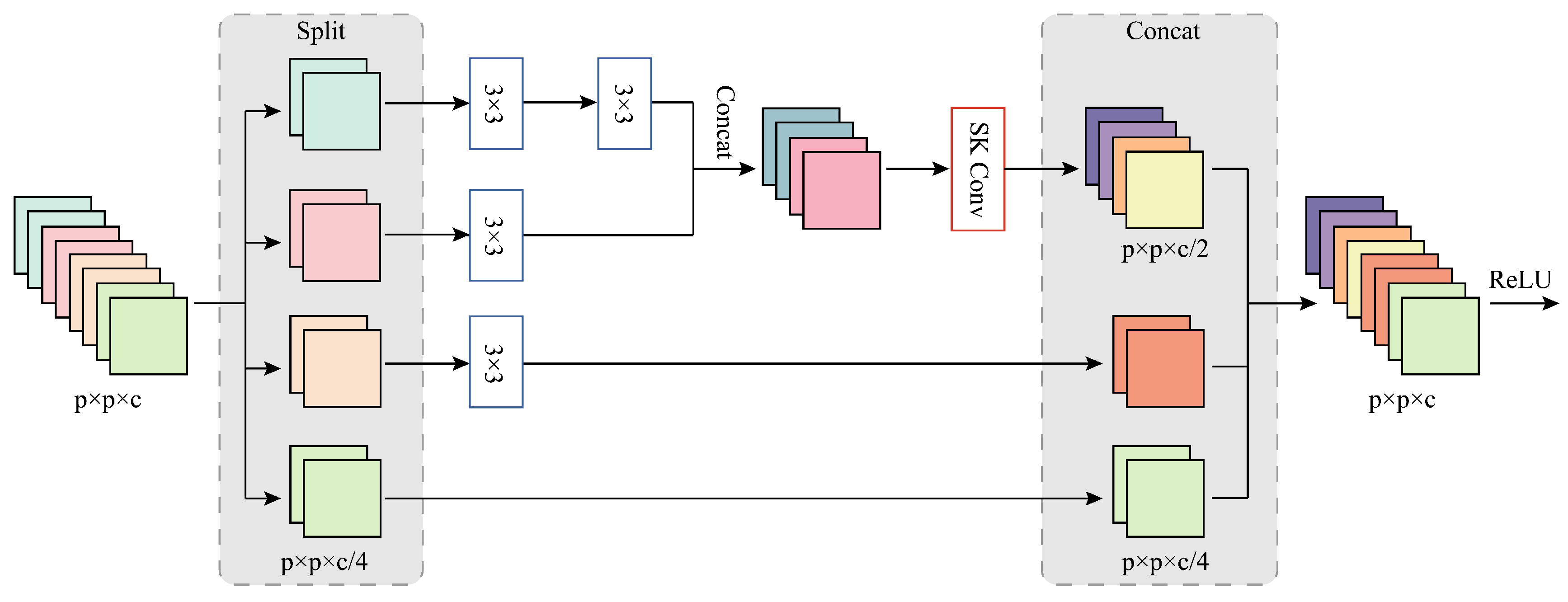
3.4. Effect of the Number of MSFE Divisions

For the MSFE module, the number of divisions s determines the maximum RF size that can be used to extract spatial features. The larger the s, the more 3 × 3 convolutions are stacked on the branch, and the larger the RF of the convolutional layer to which the branch is applied. However, for different datasets, the applicable RF size varies, so in order to obtain the optimal setting of the number of MSFE divisions, we conducted experiments by taking the number of MSFE divisions s as { 2 , 3 , 4 , 5 , 6 } 
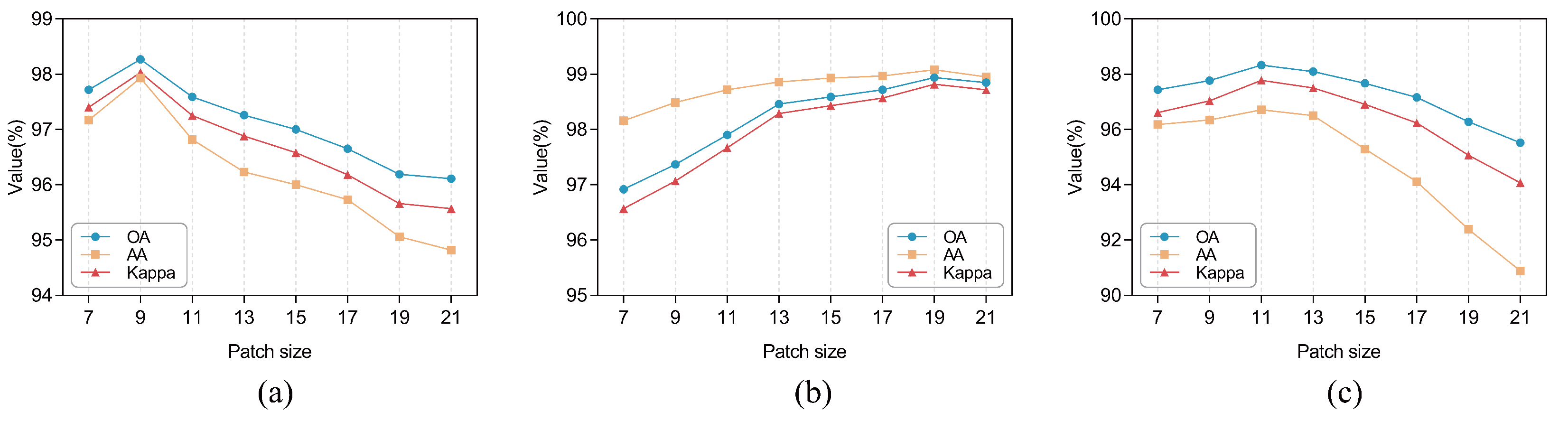
and observing the variation of OA, AA, and Kappa values of the model on the three datasets, respectively. The results of the experiment are displayed in Figure 9. It can be seen that the model performs best for the SA dataset and PU dataset when s = 4 , while for the IP dataset, s = 3 provides the best classification performance. This is because the input patches of SA and PU are larger, and their spatial information is more complex, so it is better to use a larger RF for classification, while the input patches of the IP dataset are smaller and suitable for using a relatively small RF. However, for all three datasets, the model performance tends to decrease when s = 5 and 6 because when the RF is too large, the model may incorrectly extract many useless features, confusing the classifier and possibly overfitting the model. Additionally, it can be noted that when s = 2 , the MSFE module becomes a normal residual block and can only obtain information about the 3 × 3 size RF when the OA, AA, and Kappa values are lower on all three datasets, so this verifies that our proposed MSFE module can indeed exploit the multi-scale potential at a finer level of granularity and extract spatial information from the feature maps.

3.5. Number of Groups in SSRM

The amount of groupings in SSRM determines the number of spectral bands divided and the number of parallel MSFEs to be used for feature extraction and is, therefore, a parameter to be considered. According to the experimental findings in Section 3.4, we set the number of MSFE divisions to be s = 3 on the IP dataset, and s = 4 
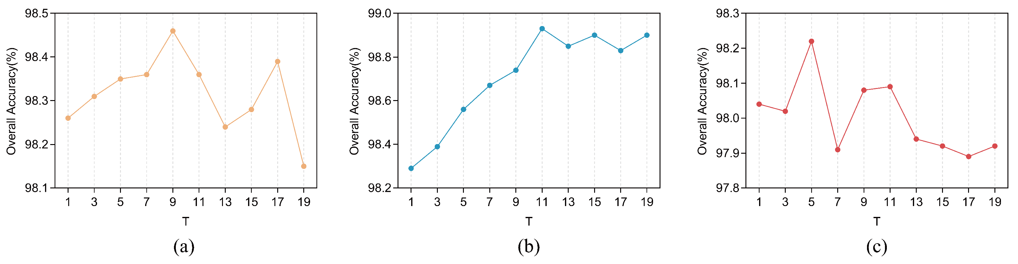
on the SA and PU datasets. On this basis, we explored the OA values on the three datasets when the number of groupings T of the SSRM takes odd values between 1 and 23, respectively. The results of the experiment are displayed in Figure 10, where it is evident that the optimal number of groups T varies for different datasets, with the optimal number of groups T being 9, 11, and 5 for the IP, SA, and PU datasets, respectively. It can be noted that when T takes the value of 1, the group convolution degenerates to a normal convolution, which is equivalent to having two global branches without local branches, and since the OA value at T = 1 is not high for all three datasets, therefore, this validates the validity of the improved grouped convolution in our presented SSRM, i.e., the validity of the local branches. Validation of the validity of global branching will be explored in a subsequent subsection on ablation studies.

3.6. Ablation Study

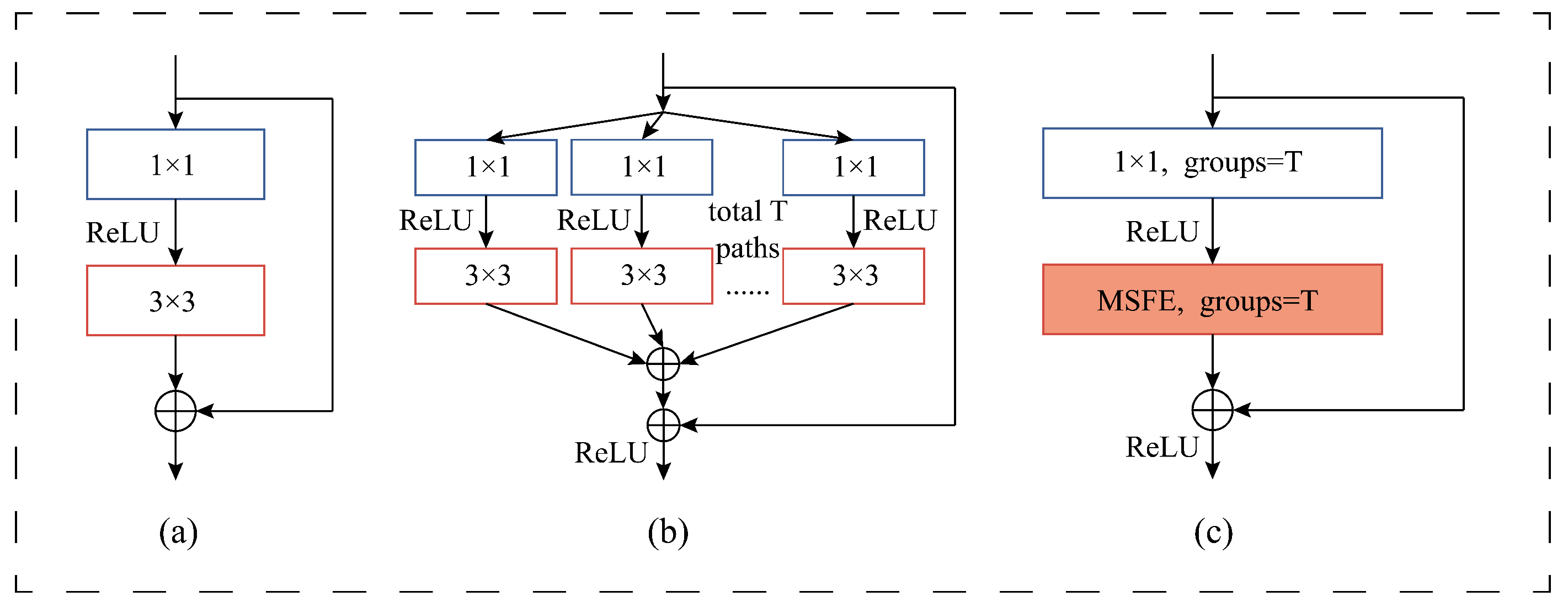
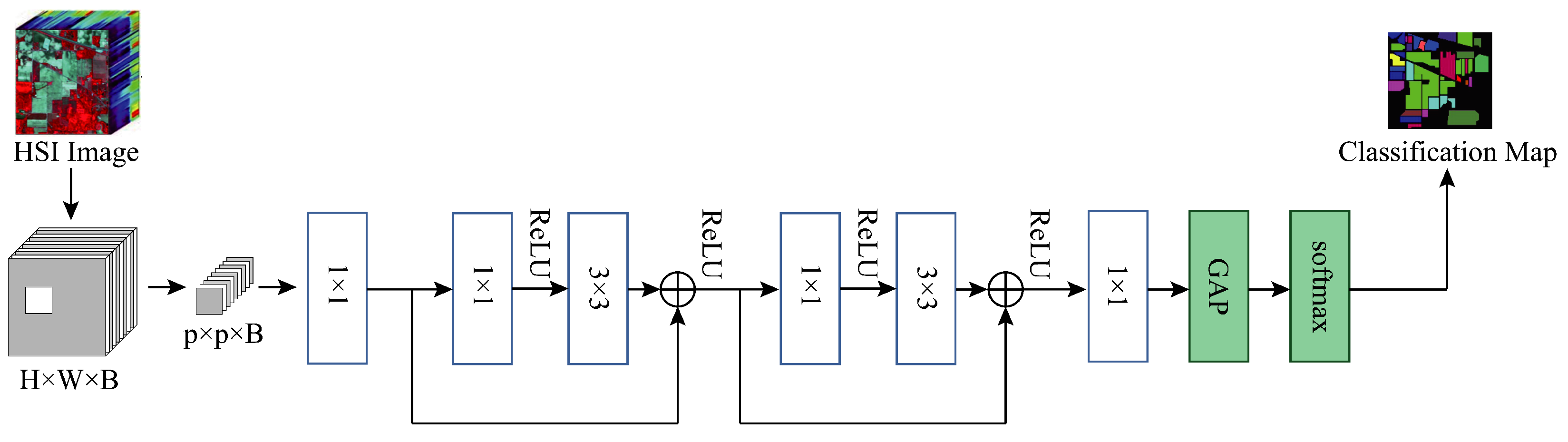
To demonstrate the contribution of the MSFE and SSRM modules of our proposed method to the final classification results of the model, we conducted an ablation study on three datasets. Specifically, we kept the other experimental settings unchanged while replacing our SSRM module with the basic module designed in DenseNet in Figure 4a, i.e., at this point the model does not use the MSFE module, the convolutions are all normal convolutions rather than grouped convolutions, and there is no global branching. We use this as the baseline model, which we name Baseline, and Figure 11 depicts the model’s construction. We add the modules we have designed to this model in turn to verify the validity of the different designs and modules.
( 1 ) 
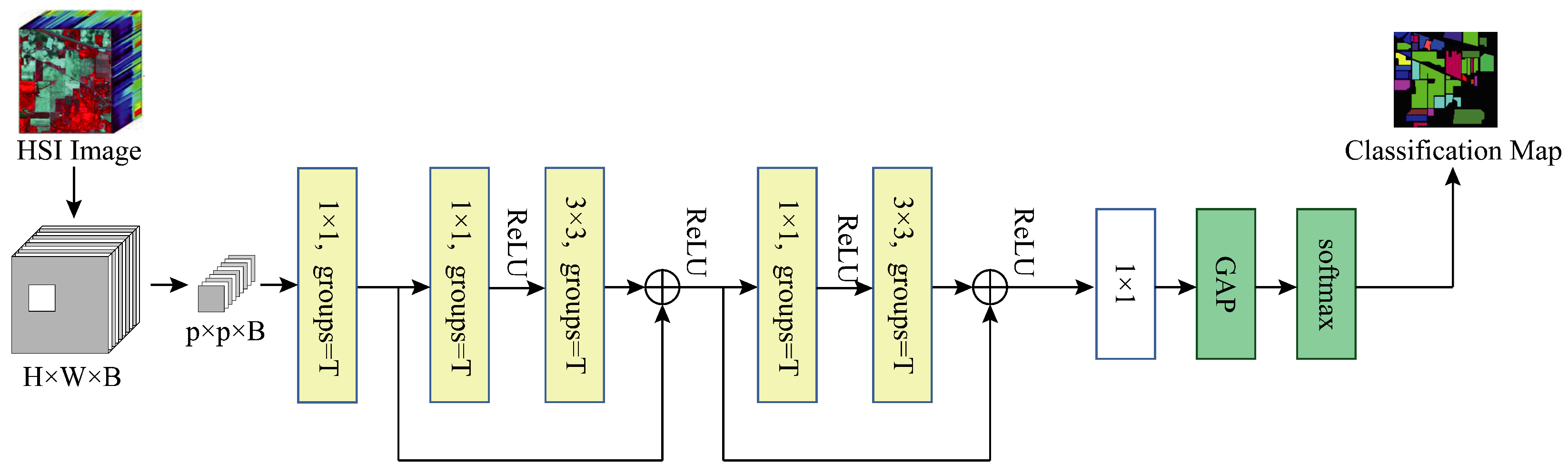
Base+GC: We replace all the convolution layers except the last one with grouped convolution on top of the Baseline to verify the effectiveness of using grouped convolution, at which point the model structure is shown in Figure 12.
( 2 ) 
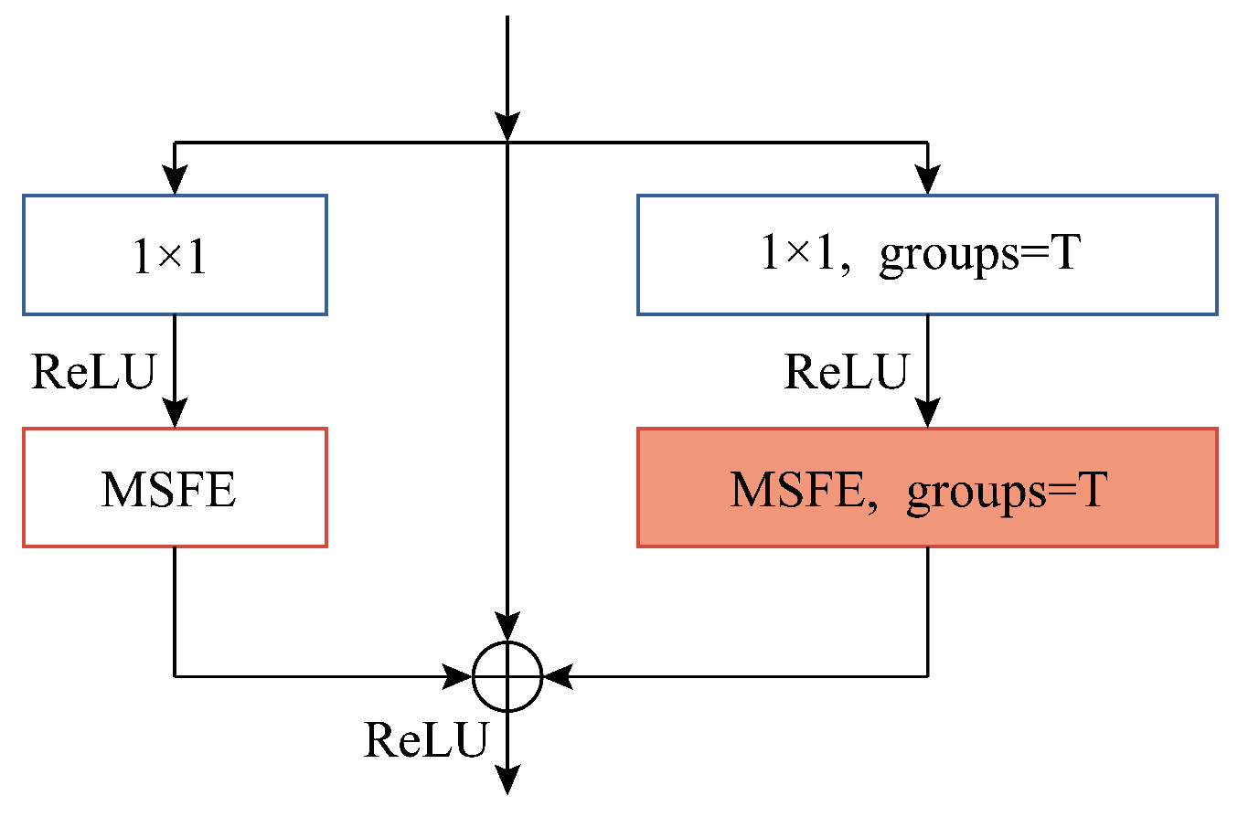
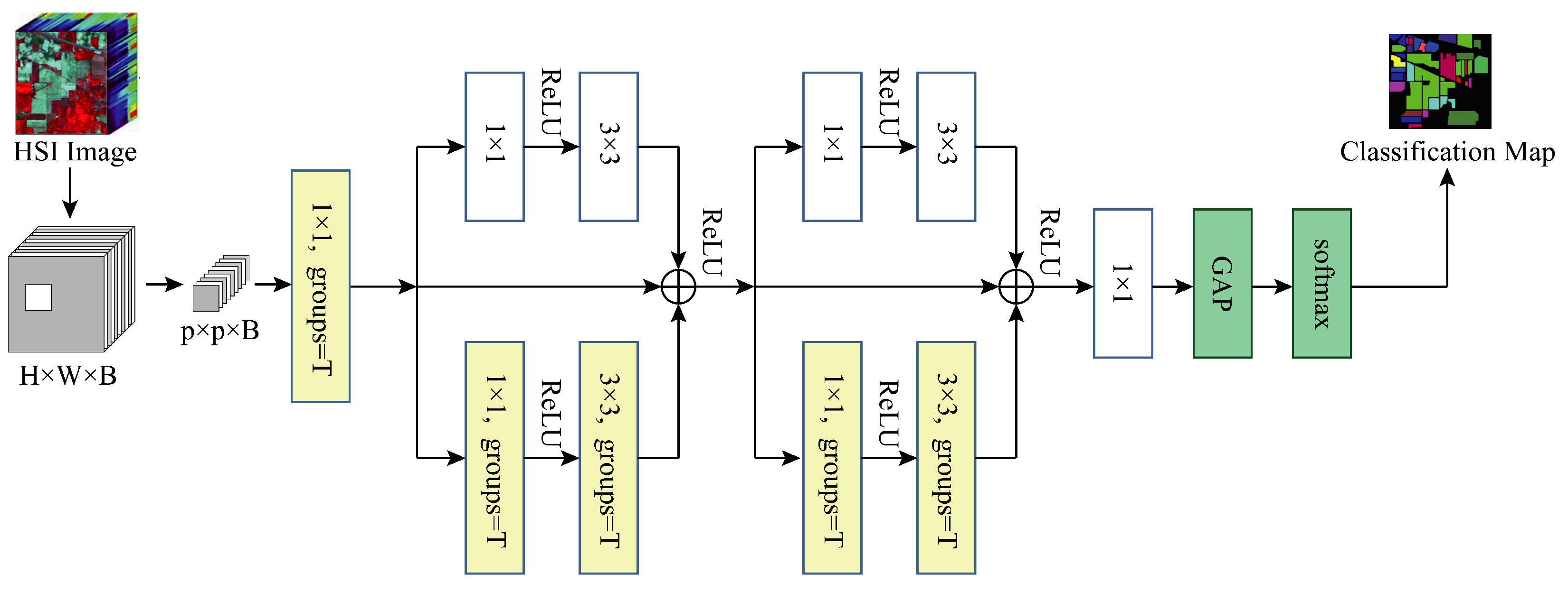
Base+GC+GB: We verify the validity of our proposed global branching by adding global branches to the two residual blocks in the model based on the use of grouped convolution, with only normal convolutional layers on the global branches, specifically a 1 × 1 kernel size convolutional layer and a 3 × 3 kernel size convolutional layer. Figure 13 illustrates the model’s current structure.
( 3 ) 
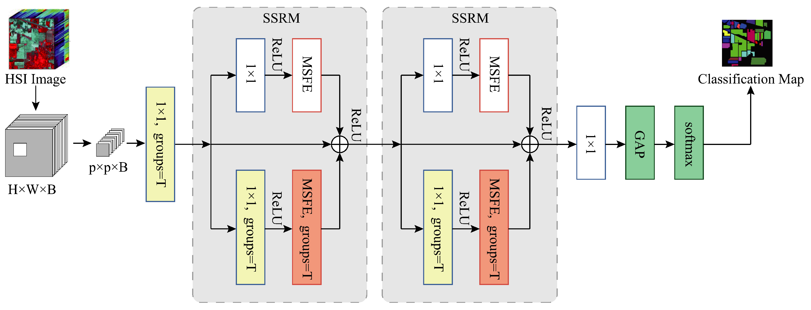
Base+GC+GB+MSFE(MFERN): We replace all the convolutional layers of kernel size 3 × 3 in the model with MSFE modules based on the use of grouped convolution and the addition of global branches, at which point the residual blocks in the model are our proposed SSRM modules and the model structure is the final structure of our presented MFERN method, as displayed in Figure 6. We can verify the effectiveness of the suggested MSFE and SSRM modules through this experiment.
Table 5 displays the findings of the ablation study using the three datasets, and it can be observed that, compared to Baseline, the addition of grouped convolution (Base+GC) to Baseline improved OA by 0.09%, AA by 0.05% and Kappa by 0.10% on the IP dataset and on the SA and PU datasets, OA, AA, and Kappa improved by 0.29%, 0.27%, 0.33%, and 0.06%, 0.09%, 0.07%, respectively. Thus, using grouped convolution instead of normal convolution is effective, especially for the SA dataset. Later, adding global branches (Base+GC+GB) to the use of grouped convolution, it can be seen that compared to Baseline, OA improves by 0.15%, AA improves by 0.29%, and Kappa improves by 0.17% on the IP dataset, OA, AA, and Kappa improve by 0.42%, 0.42%, and 0.46%, respectively, on the SA and PU datasets, 0.46% and 0.25%, 0.20% and 0.33% on the SA and PU datasets, respectively. Therefore, our proposed global branch is valid, and it is able to extract global feature information for the whole spectral band. Finally replacing all 3 × 3 kernel size convolutional layers with the MSFE module (MFERN) on top of the previous one, the OA, AA and Kappa values on all three datasets are significantly improved compared to Baseline, Specifically, for the IP dataset, OA improved by 0.30%, AA by 0.70% and Kappa by 0.34%, and for the SA and PU datasets, OA, AA, and Kappa improved by 0.52%, 0.47%, 0.58% and 0.41%, 0.50%, and 0.55%, respectively. In summary, the baseline model has the worst performance, while the performance of the model continues to improve with the addition of our suggested modules, with the best results when all of our suggested modules are used, so that the MFERN model we proposed achieves the most advanced performance.

3.7. Comparison with Other Methods

In this section, we contrast our MFERN model with other deep learning-based HSIC methods. Specifically, we compare our approach with ResNet [27], DFFN [42], SSRN [43], PResNet [29], A 2 S 2 K -ResNet [44], HybridSN [25], RSSAN [45], SSTN [46], and DCRN [47]. Among them, ResNet, DFFN, and PResNet use 2D-CNN, SSRN, A 2 S 2 K -ResNet, and RSSAN is based on 3D-CNN, HybridSN and DCRN use a hybrid CNN of 2D-CNN and 3D-CNN, and SSTN is based on Transformer. The experimental setup for this method was set up as described in Section 3.2, and the parameters were set to the values paired with the optimal experimental results in Section 3.3, Section 3.4 and Section 3.5, as follows: the IP dataset patch size of 9 × 9, the number of divisions s = 3 , and the number of groupings T = 9 ; the SA dataset patch size of 19 × 19, the number of divisions s = 4 , the number of groupings T = 11 ; the PU dataset patch size of 11 × 11, the number of divisions s = 4 , the number of groupings T = 5 . The detailed architecture of MFERN on the three datasets is shown in Table 1. The IP dataset is used as an example. All grouped convolutional layers have 288 filters in 9 groups. In other words, we divide the spectrum into 9 groups and extract features using 9 CNNs, respectively, each of which has a bandwidth of 32. The normal convolutional layer in SSRM, on the other hand, has 288 filters, and the final 1 × 1 convolutional layer has 128 filters. All the convolutional layers have a step size of 1. We chose this number of convolutional kernels in order to keep the network parameters around 10 MB on the IP and PU datasets and 50 MB on the SA dataset because of the larger input patches and higher number of subgroups in the SA dataset. For a fair comparison, the Pytorch framework was used for all compared methods; we trained the model using fewer samples, and the samples from the training, validation, and testing sets were chosen at the scale described in Section 3.1, for the IP dataset, we used 5% of the labeled samples for training, 5% for validation, and 90% for testing; for the SA and PU datasets, we used 0.5% of the labeled samples for training, 0.5% for validation, and 99% for testing. The other hyperparameters were set as described in the original paper of the model. Table 6, Table 7 and Table 8 display the outcomes of the experiment.
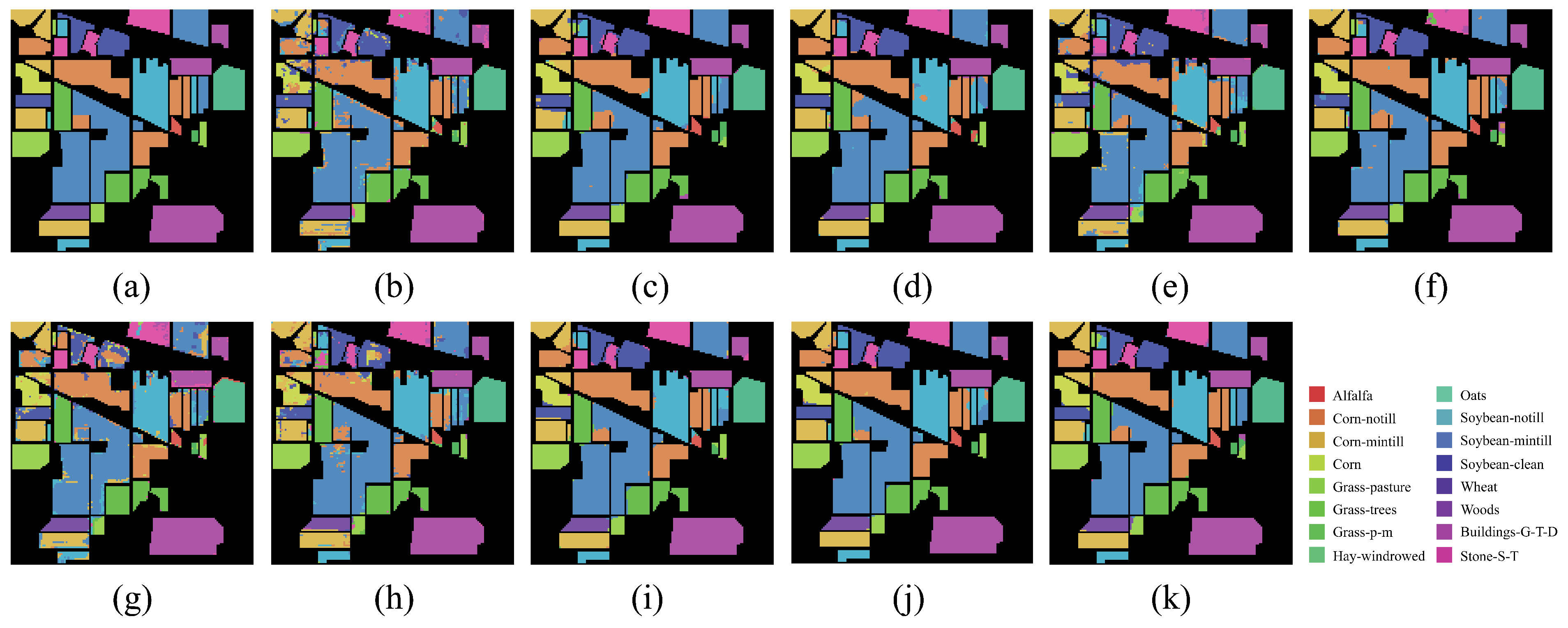
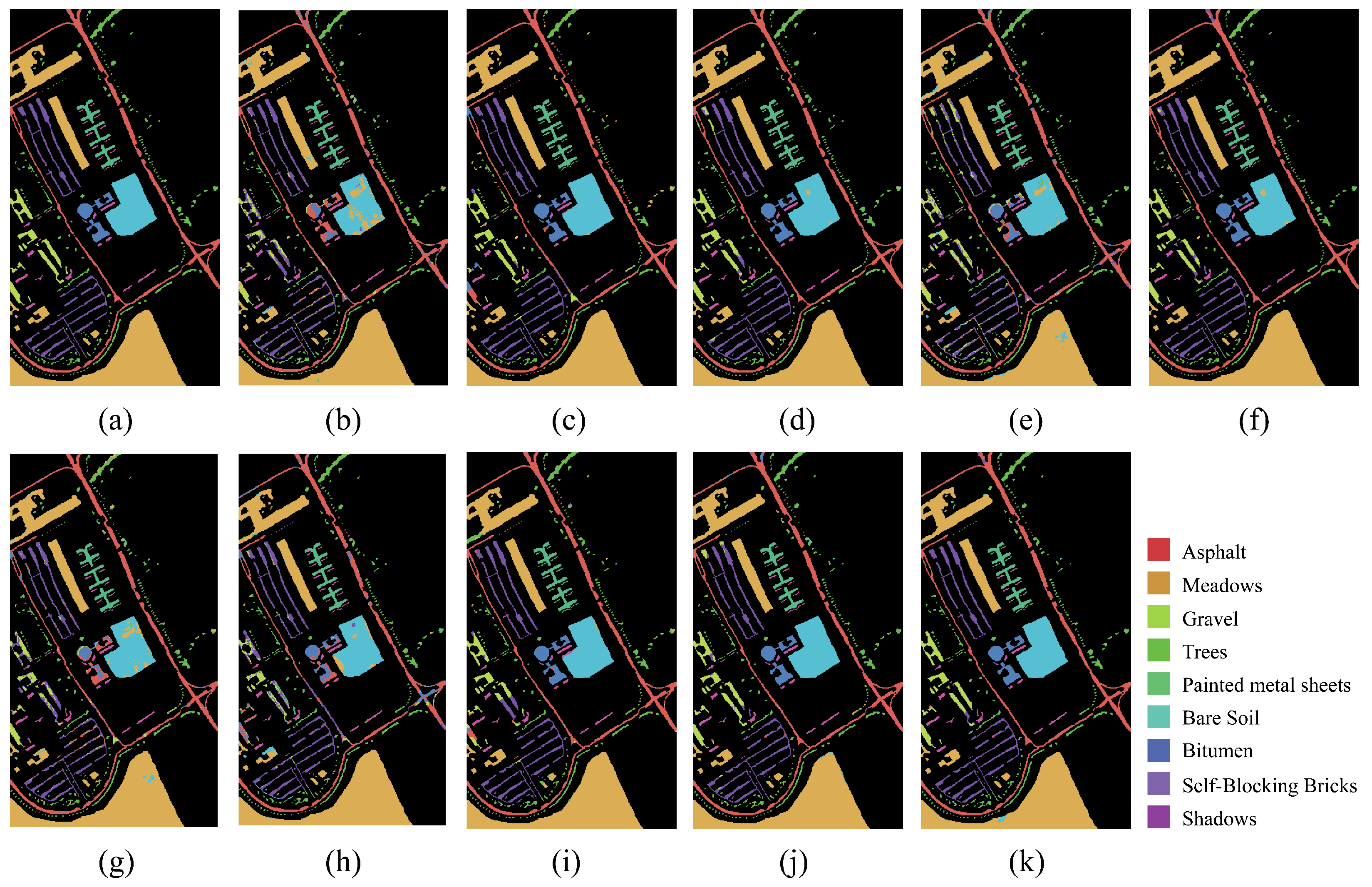
Overall, our proposed MFERN outperforms the other methods on all three datasets. Specifically, MFERN’s OA, AA, and Kappa values on the IP dataset were 98.46 ± 0.25, 98.13 ± 0.82 and 98.24 ± 0.29, respectively. On the SA and PU datasets, the OA, AA, and Kappa values were 98.94 ± 0.39, 99.08 ± 0.23, 98.82 ± 0.43 and 98.33 ± 0.47, 97.71 ± 0.28, and 97.78 ± 0.63. Compared to ResNet, DFFN, and PResNet, which are also based on 2D-CNN, MFERN has improved OA values by 2.40–9.57%, 1.70–8.01% and 3.20–10.26% over the IP, SA and PU datasets, and the above three methods are also based on residual networks, suggesting that our MSFE module helps to improve the model performance. Compared with the 3D-CNN-based SSRN, A2S2K-ResNet, MFERN’s method is closer to, but slightly better than, these two methods. This is because although we use a 2D-CNN, designing global branches in SSRM enables us to obtain spectral features for the whole band so that no spectral information is lost and obtain higher performance. Our method also performs better than the Transformer-based SSTN method; this is because we combine MSFE with group convolution in SSRM to reduce the input dimensionality of each MSFE module performing feature extraction while better extracting multi-scale spatial features, after which the features extracted from local and global branches are combined to obtain, for the full band, both spectral and multi-scale spatial features. It can be seen that the performance of RSSAN based on 3D-CNN and HybridSN based on hybrid CNN of 2D-CNN and 3D-CNN is not very good. The reason may be that the HybridSN network is more complex, which will increase the time and resource consumption for training and inference and is prone to overfitting problems, leading to unsatisfactory classification accuracy, while the RSSAN network is too simple, which may not be able to capture complex features in the data, leading to a decrease in accuracy. Taken together, networks such as RSSAN and SSTN with fewer parameters than MFERN have lower model accuracy than MFERN, which indicates that MFERN is able to keep the model complexity within a reasonable range while ensuring higher accuracy.
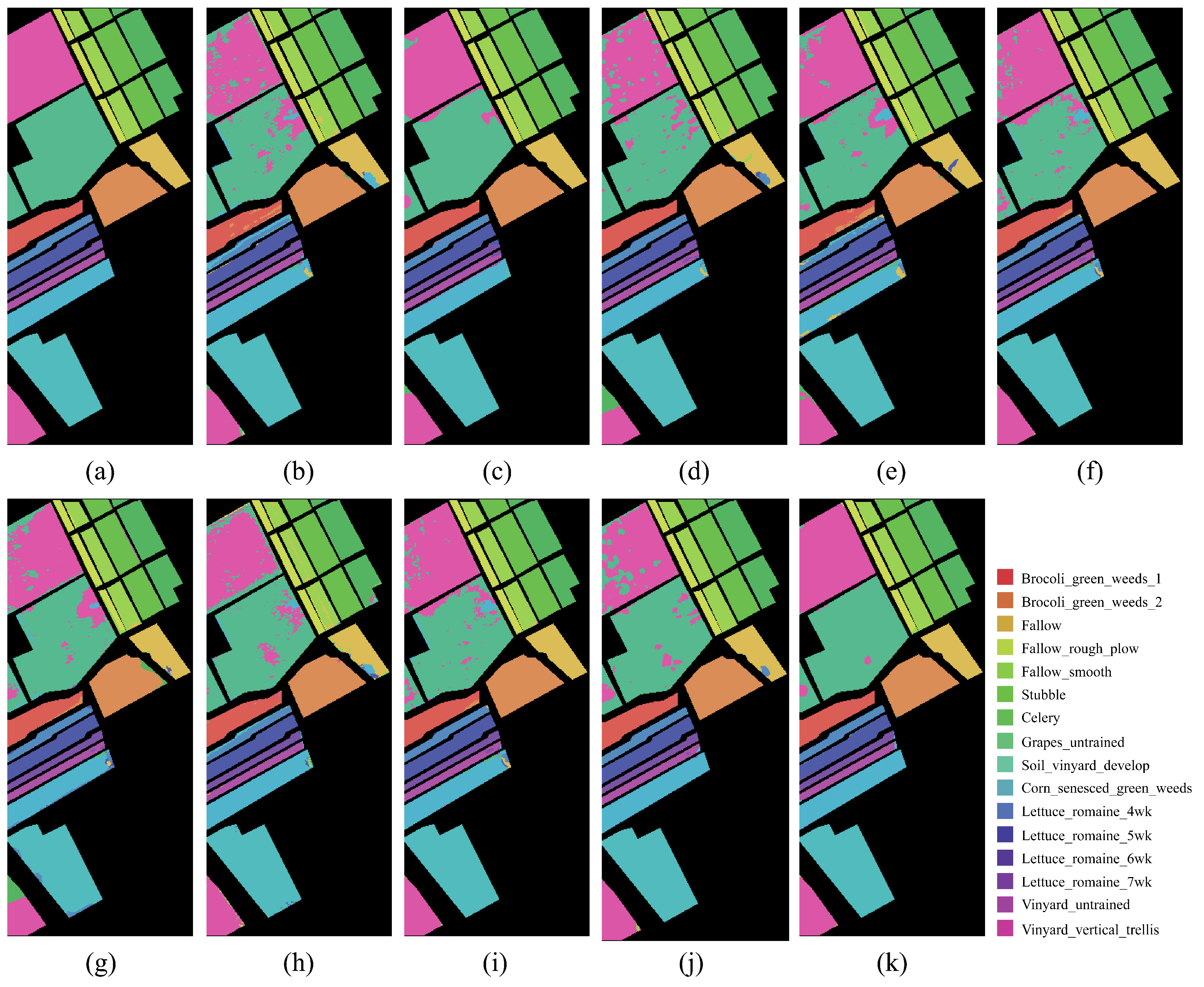
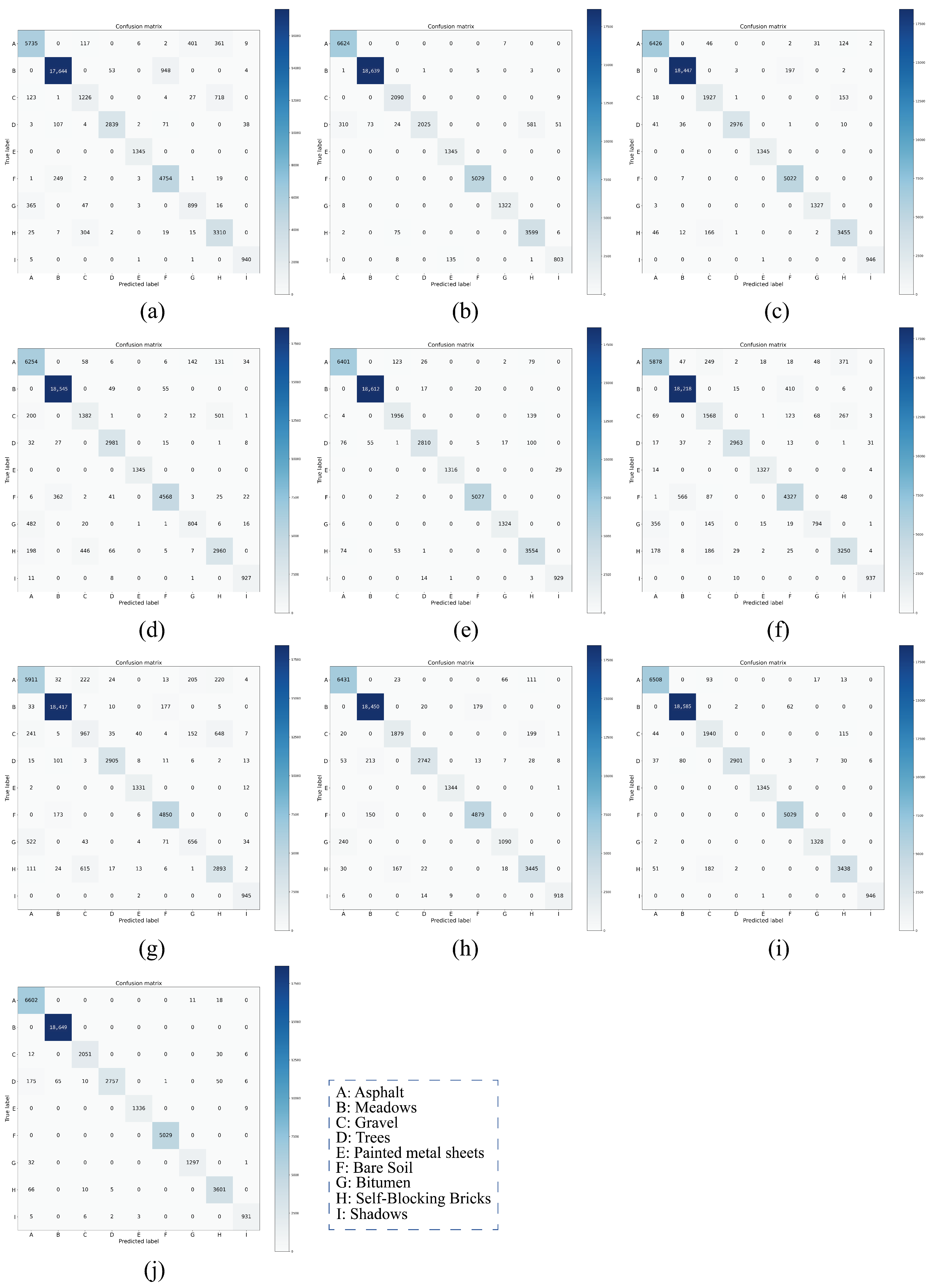
On both IP and PU datasets, compared with the DCRN model, which obtains the next best performance, the DCRN model adopts a dual-channel structure to extract spectral and spatial features of hyperspectral images separately, which may lead to a certain degree of information loss, and the correlation and interplay between spatial and spectral features may be lost when extracting both separately, which may limit the expressive power of the features. In contrast, our SSRM module captures richer feature information by designing local and global feature extraction branches, where the local branch focuses on fine-grained local structural and textural features, which can perceive the subtle changes and local information of the target object, thus enhancing the robustness of the model against noise, occlusion, and other disturbing factors. The global branch, on the other hand, can obtain the overall contextual information, providing a grasp of the overall features of the image and improving the classification accuracy and robustness. On the SA dataset, the DFFN network is deeper and extracts deeper features compared to the DFFN model that obtains the next best performance but ignores the fact that different sizes of features are subject to different RF and only uses a fixed-size RF for feature extraction, which restricts the learning weight of the model. Our MSFE module solves this problem well, and the multi-scale feature extraction branch provides different sizes of receptive fields to extract feature information at different scales and also considers the spatial relationship between pixels through the receptive fields at different scales, which helps the model to better understand the spatial distribution characteristics of the target object and improve the classification accuracy. Therefore, MFERN is more robust, does not need to stack too many blocks to fully extract the feature information, ensures high accuracy in the case of small samples, and keeps the model complexity at a low level. To check the classification performance more visually, we plotted the classification maps and confusion matrix plots produced using different methodologies on the three datasets, as shown in Figure 14, Figure 15, Figure 16, Figure 17, Figure 18 and Figure 19. On all three datasets, MFERN has a high classification accuracy with a low noise level.
We further assessed the performance variation of the different methods when using different training sample percentages; specifically, for the IP dataset, we explored the variation of OA values for each method when the training sample size was taken from 6–10%, and for the SA dataset and PU dataset, we explored the variation of OA values for each method when the training sample size was taken from 1–5%. Figure 20 displays the experimental results.
It can be seen that HybridSN performs poorly on the IP dataset, ResNet gives a poor performance on the SA dataset, and RSSAN gives poor classification accuracy on the PU dataset, while DFFN and DCRN have a more stable performance on all three datasets. The method in this study significantly outperforms the other comparative methods even with a small training sample set, which shows that MFERN can fully extract the spatial and spectral features of hyperspectral images, making it have high classification accuracy even with a small sample size. The performance gap between the methods gradually closes as the training sample size increases, yet our suggested method consistently outperforms the other approaches on the three datasets. This demonstrates the strong robustness of our proposed MFERN approach.
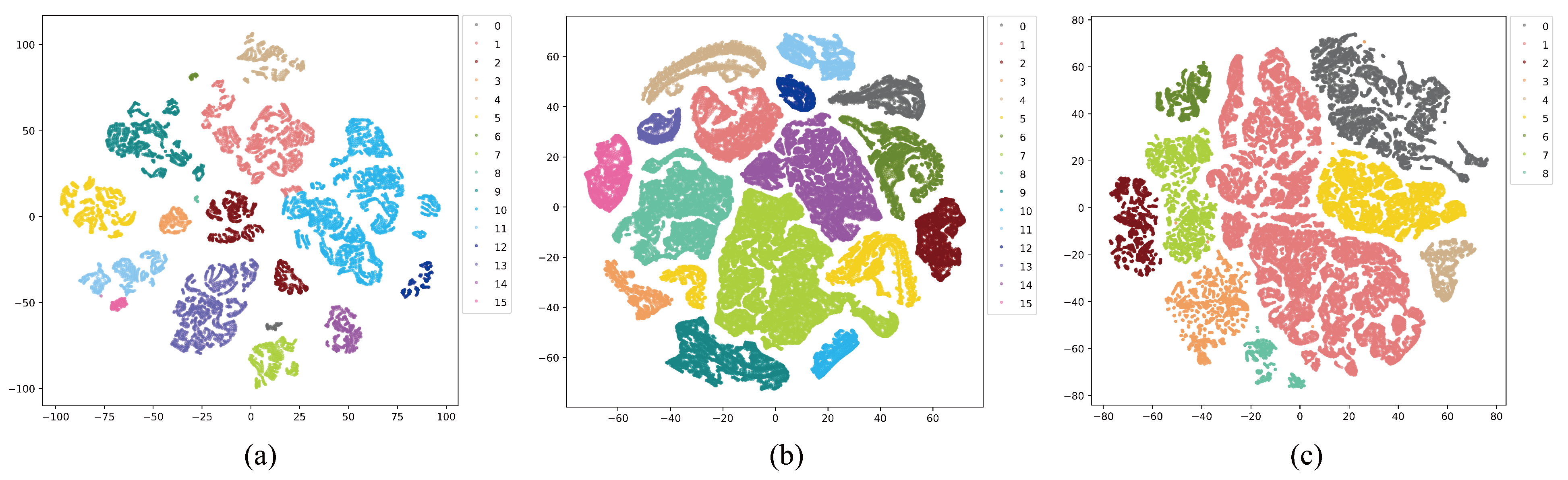
To validate the feature extraction capability of our proposed MSFE and SSRM and the representation capability of our trained models, we visualized the 2D spectral space features proposed by the test samples in the three datasets through the t-SNE algorithm [48], as depicted in Figure 21. In the figure, samples from the same class are clustered into one group, while samples from different classes are kept apart, and samples from different classes are shown using different colors are shown. The figure shows that on the three datasets, the samples from various classes are more clearly distinguished, thus indicating that our MSFE extracts feature more adequately at the fine- and coarse-grained levels and that our MFERN model can learn abstract representations of spectral space features well and with high classification accuracy.

4. Discussion

In our extensive experiments on three different HSI datasets, the parameter experiments allowed us to determine the optimal parameter settings for model training; the ablation experiments verified the validity of our proposed module; and the comparison experiments with other models showed that our proposed model achieves the best performance in terms of OA, AA, and Kappa values, especially when the size of the training samples is small; our model’s performance advantage is more obvious, which is mainly based on the following reasons. Firstly, our proposed MSFE module has strong adaptive ability, which can fully extract the multi-scale features of the image; secondly, the combination of local branching and global branching of the SSRM module can fully exploit the spatial and spectral features of hyperspectral images; lastly, the combination of the above modules allows the proposed method to fully extract the feature information without stacking a large number of blocks repeatedly, which keeps the number of parameters of the proposed method under reasonable control. The number of parameters of the proposed method is controlled within a reasonable range.
Although the proposed method achieves good performance in hyperspectral image classification, it has the following limitations.
(1)
The proposed method is more suitable for hyperspectral images with a large number of channels, and the group convolution setting can extract the feature information on different channels while reducing the number of parameters. However, for images with a small number of channels, this setup is a little ribbed and should be improved with specific problems.
(2)
The complexity of the proposed method is not completely dominant; although it is lower than most of the comparison models, it is still slightly higher than SSTN and other models, which can be improved later.
In order to address the above limitations, we will further improve the proposed method in our future work.

5. Conclusions

In this paper, a spectral segmentation-based multi-scale spatial feature extraction residual network (MFERN) is proposed for hyperspectral image classification. The network consists of a multi-scale spatial feature extraction module (MSFE) and a spectral segmentation residual module (SSRM). The MSFE divides the spectral bands of the input image into multiple non-overlapping sub-bands and processes each sub-band using spatial spectral feature extraction branches with different RFs. We increase the RFs of the branches by stacking convolution kernels of 3 × 3 size and using “selective kernel” convolution to improve the adaptive capability of the model. SSRM combines the MSFE module with dense block-based group convolution and adds a global branch to the original residual structure to synthesize spatial-spectral information of the extracted feature maps. We conducted extensive experiments on three different HSI datasets, and the comparison experiments with other models show that our proposed model has a more obvious performance advantage when using fewer training samples, which suggests that our proposed module is able to adequately extract the feature information of hyperspectral images, and thus has a higher classification accuracy. Although the performance gap between the methods gradually narrows as the number of training samples increases, our MFERN model consistently outperforms the other methods on all three datasets. Possible future research directions include the design of effective spectral attention modules and the fusion of 2D and 3D CNNs in the network.

Author Contributions

All the authors made important contributions to this work. Among them, J.W., J.R. and Y.P. designed the study, analyzed the results, and completed the validation work. M.S. provided suggestions for the revision of the paper. All authors have read and agreed to the published version of the manuscript.

Funding

This research received no external funding.

Data Availability Statement

The datasets generated during and/or analyzed during the current study are available from the corresponding author on reasonable request.

Conflicts of Interest

The authors declare no conflict of interest.

References

  1. Landgrebe, D. Hyperspectral image data analysis. IEEE Signal Process. Mag. 2002, 19, 17–28. [Google Scholar] [CrossRef]
  2. Ma, X.; Fu, A.; Wang, J.; Wang, H.; Yin, B. Hyperspectral image classification based on deep deconvolution network with skip architecture. IEEE Trans. Geosci. Remote Sens. 2018, 56, 4781–4791. [Google Scholar] [CrossRef]
  3. Bhosle, K.; Musande, V. Evaluation of deep learning CNN model for land use land cover classification and crop identification using hyperspectral remote sensing images. J. Indian Soc. Remote Sens. 2019, 47, 1949–1958. [Google Scholar] [CrossRef]
  4. Yan, Z.; Zhang, H.; Piramuthu, R.; Jagadeesh, V.; DeCoste, D.; Di, W.; Yu, Y. HD-CNN: Hierarchical deep convolutional neural networks for large scale visual recognition. In Proceedings of the IEEE International Conference on Computer Vision (ICCV), Santiago, Chile, 7–13 December 2015; pp. 2740–2748. [Google Scholar]
  5. Liu, M.; Zhao, J.; Li, G.; Zhang, H.; Wu, T. Tongue coat information extraction of the Traditional Chinese Medicine with hyperspectral image. Guang Pu Xue Yu Guang Pu Fen Xi 2017, 37, 162–165. [Google Scholar]
  6. Ren, J.; Wang, R.; Liu, G.; Wang, Y.; Wu, W. An SVM-based nested sliding window approach for spectral–spatial classification of hyperspectral images. Remote Sens. 2021, 13, 114. [Google Scholar] [CrossRef]
  7. Zhao, Y.; Qian, Y.; Li, C. Improved KNN text classification algorithm with mapReduce implementation. In Proceedings of the International Conference on Systems and Informatics (ICSAI), Hangzhou, China, 11–13 November 2017; pp. 1417–1422. [Google Scholar]
  8. Khodadadzadeh, M.; Ghamisi, P.; Contreras, C.; Gloaguen, R. Subspace multinomial logistic regression ensemble for classification of hyperspectral images. In Proceedings of the IEEE International Geoscience and Remote Sensing Symposium (IGARSS), Valencia, Spain, 22–27 July 2018; pp. 5740–5743. [Google Scholar]
  9. Donoho, D.L. High-dimensional data analysis: The curses and blessings of dimensionality. AMS Math. Chall. Lect. 2000, 1, 32. [Google Scholar]
  10. Ren, J.; Wang, R.; Liu, G.; Feng, R.; Wang, Y.; Wu, W. Partitioned relief-F method for dimensionality reduction of hyperspectral images. Remote Sens. 2020, 12, 1104. [Google Scholar] [CrossRef]
  11. Hong, D.; Yokoya, N.; Chanussot, J.; Xu, J.; Zhu, X.X. Joint and progressive subspace analysis (JPSA) with spatial–spectral manifold alignment for semisupervised hyperspectral dimensionality reduction. IEEE Trans. Cybern. 2020, 51, 3602–3615. [Google Scholar] [CrossRef]
  12. Duan, Y.; Huang, H.; Tang, Y. Local constraint-based sparse manifold hypergraph learning for dimensionality reduction of hyperspectral image. IEEE Trans. Geosci. Remote Sens. 2020, 59, 613–628. [Google Scholar] [CrossRef]
  13. Zhong, S.; Zhang, Y.; Chang, C.-I. A spectral–spatial feedback close network system for hyperspectral image classification. IEEE Trans. Geosci. Remote Sens. 2019, 57, 10056–10069. [Google Scholar] [CrossRef]
  14. Duan, P.; Kang, X.; Li, S.; Ghamisi, P.; Benediktsson, J.A. Fusion of multiple edge-preserving operations for hyperspectral image classification. IEEE Trans. Geosci. Remote Sens. 2019, 57, 10336–10349. [Google Scholar] [CrossRef]
  15. Zhang, X.; Wei, Y.; Cao, W.; Yao, H.; Peng, J.; Zhou, Y. Local correntropy matrix representation for hyperspectral image classification. IEEE Trans. Geosci. Remote Sens. 2022, 60, 1–13. [Google Scholar] [CrossRef]
  16. Ghamisi, P.; Benediktsson, J.A.; Cavallaro, G.; Plaza, A. Automatic framework for spectral–spatial classification based on supervised feature extraction and morphological attribute profiles. IEEE Trans. Geosci. Remote Sens. 2014, 52, 5771–5782. [Google Scholar] [CrossRef]
  17. Pan, C.; Gao, X.; Wang, Y.; Li, J. Markov random fields integrating adaptive interclass-pair penalty and spectral similarity for hyperspectral image classification. IEEE Trans. Geosci. Remote Sens. 2019, 57, 2520–2534. [Google Scholar] [CrossRef]
  18. Jia, S.; Deng, X.; Zhu, J.; Xu, M.; Zhou, J.; Jia, X. Collaborative representation-based multiscale superpixel fusion for hyperspectral image classification. IEEE Trans. Geosci. Remote Sens. 2019, 57, 7770–7784. [Google Scholar] [CrossRef]
  19. Zhou, P.; Han, J.; Cheng, G.; Zhang, B. Learning compact and discriminative stacked autoencoder for hyperspectral image classification. IEEE Trans. Geosci. Remote Sens. 2019, 57, 4823–4833. [Google Scholar] [CrossRef]
  20. Chen, Y.; Jiang, H.; Li, C.; Jia, X.; Ghamisi, P. Deep feature extraction and classification of hyperspectral images based on convolutional neural networks. IEEE Trans. Geosci. Remote Sens. 2016, 54, 6232–6251. [Google Scholar] [CrossRef]
  21. Dong, S.; Feng, W.; Quan, Y.; Dauphin, G.; Gao, L.; Xing, M. Deep ensemble CNN method based on sample expansion for hyperspectral image classification. IEEE Trans. Geosci. Remote Sens. 2022, 60, 1–15. [Google Scholar] [CrossRef]
  22. Mou, L.; Ghamisi, P.; Zhu, X.X. Deep recurrent neural networks for hyperspectral image classification. IEEE Trans. Geosci. Remote Sens. 2017, 55, 3639–3655. [Google Scholar] [CrossRef]
  23. Liu, B.; Yu, X.; Zhang, P.; Tan, X.; Yu, A.; Xue, Z. A semi-supervised convolutional neural network for hyperspectral image classification. Remote Sens. Lett. 2017, 8, 839–848. [Google Scholar] [CrossRef]
  24. Yu, C.; Han, R.; Song, M.; Liu, C.; Chang, C.-I. A simplified 2D-3D CNN architecture for hyperspectral image classification based on spatial–spectral fusion. IEEE J. Sel. Top. Appl. Earth Obs. Remote Sens. 2020, 13, 2485–2501. [Google Scholar] [CrossRef]
  25. Roy, S.K.; Krishna, G.; Dubey, S.R.; Chaudhuri, B.B. HybridSN: Exploring 3-D–2-D CNN feature hierarchy for hyperspectral image classification. IEEE Geosci. Remote Sens. Lett. 2019, 17, 277–281. [Google Scholar] [CrossRef]
  26. Srivastava, R.K.; Greff, K.; Schmidhuber, J. Training very deep networks. In Proceedings of the Advances in Neural Information Processing Systems 28 (NIPS 2015), Montreal, QC, Canada, 7–12 December 2015. [Google Scholar]
  27. He, K.; Zhang, X.; Ren, S.; Sun, J. Deep residual learning for image recognition. In Proceedings of the IEEE Conference on Computer Vision and Pattern Recognition (CVPR), Las Vegas, NV, USA, 26 June–1 July 2016; pp. 770–778. [Google Scholar]
  28. Huang, G.; Liu, Z.; Van Der Maaten, L.; Weinberger, K.Q. Densely connected convolutional networks. In Proceedings of the IEEE Conference on Computer Vision and Pattern Recognition (CVPR), Honolulu, HI, USA, 21–26 July 2017; pp. 4700–4708. [Google Scholar]
  29. Paoletti, M.E.; Haut, J.M.; Fernandez-Beltran, R.; Plaza, J.; Plaza, A.J.; Pla, F. Deep pyramidal residual networks for spectral–spatial hyperspectral image classification. IEEE Trans. Geosci. Remote Sens. 2018, 57, 740–754. [Google Scholar] [CrossRef]
  30. Li, R.; Zheng, S.; Duan, C.; Yang, Y.; Wang, X. Classification of hyperspectral image based on double-branch dual-attention mechanism network. Remote Sens. 2020, 12, 582. [Google Scholar] [CrossRef]
  31. Wu, Y.; Zhou, T.; Hu, X.; Shi, L.; Yang, W. RepSSRN: The structural reparameterization applied to SSRN for hyperspectral image classification. IEEE Geosci. Remote Sens. Lett. 2022, 19, 1–5. [Google Scholar] [CrossRef]
  32. Lee, Y.; Jung, H.; Han, D.; Kim, K.; Kim, J. Learning receptive field size by learning filter size. In Proceedings of the 2019 IEEE Winter Conference on Applications of Computer Vision (WACV), Waikoloa Village, HI, USA, 7–11 January 2019; pp. 1203–1212. [Google Scholar]
  33. Li, X.; Wang, W.; Hu, X.; Yang, J. Selective kernel networks. In Proceedings of the IEEE/CVF Conference on Computer Vision and Pattern Recognition, Long Beach, CA, USA, 16–17 June 2019; pp. 510–519. [Google Scholar]
  34. Xie, S.; Girshick, R.; Dollár, P.; Tu, Z.; He, K. Aggregated residual transformations for deep neural networks. In Proceedings of the IEEE Conference on Computer Vision and Pattern Recognition (CVPR), Honolulu, HI, USA, 21–26 July 2017; pp. 1492–1500. [Google Scholar]
  35. Szegedy, C.; Vanhoucke, V.; Ioffe, S.; Shlens, J.; Wojna, Z. Rethinking the inception architecture for computer vision. In Proceedings of the IEEE Conference on Computer Vision and Pattern Recognition (CVPR), Las Vegas, NV, USA, 26 June–1 July 2016; pp. 2818–2826. [Google Scholar]
  36. Ioffe, S.; Szegedy, C. Batch normalization: Accelerating deep network training by reducing internal covariate shift. In Proceedings of the International Conference on Machine Learning, Lille, France, 7–9 July 2015; pp. 448–456. [Google Scholar]
  37. Nair, V.; Hinton, G.E. Rectified linear units improve restricted boltzmann machines. In Proceedings of the 27th International Conference on Machine Learning (ICML), Haifa, Israel, 21–24 June 2010; pp. 807–814. [Google Scholar]
  38. Lin, M.; Chen, Q.; Yan, S. Network in Network. In Proceedings of the IEEE International Conference on Learning Representations, Columbus, OH, USA, 23–28 June 2014; pp. 1–10. [Google Scholar]
  39. Green, R.O.; Eastwood, M.L.; Sarture, C.M.; Chrien, T.G.; Aronsson, M.; Chippendale, B.J.; Faust, J.A.; Pavri, B.E.; Chovit, C.J.; Solis, M. Imaging spectroscopy and the airborne visible/infrared imaging spectrometer (AVIRIS). Remote Sens. Environ. 1998, 65, 227–248. [Google Scholar] [CrossRef]
  40. Kunkel, B.; Blechinger, F.; Lutz, R.; Doerffer, R.; Van der Piepen, H.; Schroder, M. ROSIS (Reflective optics system imaging spectrometer)-A candidate instrument for polar platform missions. In Proceedings of the Optoelectronic Technologies for Remote Sensing from Space, Cannes, France, 19–20 November 1987; pp. 134–141. [Google Scholar]
  41. Diederik, K.; Jimmy, B. Adam: A method for stochastic optimization. In Proceedings of the 3rd International Conference on Learning Representations, San Diego, CA, USA, 7–9 May 2015; pp. 1–13. [Google Scholar]
  42. Song, W.; Li, S.; Fang, L.; Lu, T. Hyperspectral image classification with deep feature fusion network. IEEE Trans. Geosci. Remote Sens. 2018, 56, 3173–3184. [Google Scholar] [CrossRef]
  43. Zhong, Z.; Li, J.; Luo, Z.; Chapman, M. Spectral–spatial residual network for hyperspectral image classification: A 3-D deep learning framework. IEEE Trans. Geosci. Remote Sens. 2017, 56, 847–858. [Google Scholar] [CrossRef]
  44. Roy, S.K.; Manna, S.; Song, T.; Bruzzone, L. Attention-based adaptive spectral–spatial kernel ResNet for hyperspectral image classification. IEEE Trans. Geosci. Remote Sens. 2020, 59, 7831–7843. [Google Scholar] [CrossRef]
  45. Zhu, M.; Jiao, L.; Liu, F.; Yang, S.; Wang, J. Residual spectral–spatial attention network for hyperspectral image classification. IEEE Trans. Geosci. Remote Sens. 2020, 59, 449–462. [Google Scholar] [CrossRef]
  46. Zhong, Z.; Li, Y.; Ma, L.; Li, J.; Zheng, W.-S. Spectral–spatial transformer network for hyperspectral image classification: A factorized architecture search framework. IEEE Trans. Geosci. Remote Sens. 2021, 60, 1–15. [Google Scholar] [CrossRef]
  47. Xu, Y.; Li, Z.; Li, W.; Du, Q.; Liu, C.; Fang, Z.; Zhai, L. Dual-channel residual network for hyperspectral image classification with noisy labels. IEEE Trans. Geosci. Remote Sens. 2022, 60, 1–11. [Google Scholar] [CrossRef]
  48. Van der Maaten, L.; Hinton, G. Visualizing data using t-SNE. J. Mach. Learn. Res. 2008, 9, 2579–2605. [Google Scholar]
Figure 1. Multi-scale spatial feature extraction module (with s = 4 as an example).
Remotesensing 15 04219 g001
Figure 2. Small networks replacing 5 × 5 convolution. (a) 5 × 5 convolution results, (b) 3 × 3 convolution results.
Remotesensing 15 04219 g002
Figure 3. Selective kernel convolution.
Remotesensing 15 04219 g003
Figure 4. (a) basic module designed in DenseNet, (b) aggregated residual transform, (c) equivalent implementation by using group convolution with group number equal to T.
Remotesensing 15 04219 g004
Figure 5. Spectral Segmentation Residual Module (SSRM).
Remotesensing 15 04219 g005
Figure 6. A general framework for a spectral segmentation-based multi-scale spatial feature extraction residual network (MFERN).
Remotesensing 15 04219 g006
Figure 7. Variation curves of the validation set OA values with increasing epoch on the (a) IP dataset, (b) SA dataset, and (c) PU dataset.
Remotesensing 15 04219 g007
Figure 8. Classification results using various patch sizes on the (a) IP dataset, (b) SA dataset and (c) PU dataset.
Remotesensing 15 04219 g008
Figure 9. Classification results using various number of MSFE divisions s on the (a) IP dataset, (b) SA dataset and (c) PU dataset.
Remotesensing 15 04219 g009
Figure 10. Classification results using different numbers of SSRM groups T on the (a) IP dataset, (b) SA dataset and (c) PU dataset.
Remotesensing 15 04219 g010
Figure 11. Baseline model structure.
Remotesensing 15 04219 g011
Figure 12. Base+GC model structure.
Remotesensing 15 04219 g012
Figure 13. Base+GC+GB model structure.
Remotesensing 15 04219 g013
Figure 14. Classification map of the IP dataset. (a) Ground truth map. (b) ResNet. (c) DFFN. (d) SSRN. (e) PResNet. (f) A 2 S 2 K -ResNet. (g) HybridSN. (h) RSSAN. (i) SSTN. (j) DCRN. (k) MFERN.
Remotesensing 15 04219 g014
Figure 15. Classification map of the SA dataset. (a) Ground truth map. (b) ResNet. (c) DFFN. (d) SSRN. (e) PResNet. (f) A 2 S 2 K -ResNet. (g) HybridSN. (h) RSSAN. (i) SSTN. (j) DCRN. (k) MFERN.
Remotesensing 15 04219 g015
Figure 16. Classification map of the PU dataset. (a) Ground truth map. (b) ResNet. (c) DFFN. (d) SSRN. (e) PResNet. (f) A 2 S 2 K -ResNet. (g) HybridSN. (h) RSSAN. (i) SSTN. (j) DCRN. (k) MFERN.
Remotesensing 15 04219 g016
Figure 17. Confusion matrix plot for the IP dataset. (a) ResNet. (b) DFFN. (c) SSRN. (d) PResNet. (e) A 2 S 2 K -ResNet. (f) HybridSN. (g) RSSAN. (h) SSTN. (i) DCRN. (j) MFERN.
Remotesensing 15 04219 g017
Figure 18. Confusion matrix plot for the SA dataset. (a) ResNet. (b) DFFN. (c) SSRN. (d) PResNet. (e) A 2 S 2 K -ResNet. (f) HybridSN. (g) RSSAN. (h) SSTN. (i) DCRN. (j) MFERN.
Remotesensing 15 04219 g018
Figure 19. Confusion matrix plot for the PU dataset. (a) ResNet. (b) DFFN. (c) SSRN. (d) PResNet. (e) A 2 S 2 K -ResNet. (f) HybridSN. (g) RSSAN. (h) SSTN. (i) DCRN. (j) MFERN.
Remotesensing 15 04219 g019
Figure 20. Overall accuracy of different methods on the (a) IP dataset, (b) SA dataset, and (c) PU dataset with different ratios of training samples.
Remotesensing 15 04219 g020
Figure 21. Visualisation results of the t-SNE algorithm on the (a) IP dataset, (b) SA dataset and (c) PU dataset. The test sample features are represented by the dots, whose category labels are indicated by different colors.
Remotesensing 15 04219 g021
Table 1. MFERN structure on the IP, SA, and PU datasets.
LayerIPSAPU
1 × 1 *200; T = 9 , padding = 1; 288204; T = 11 , padding = 1; 297103; T = 11 , padding = 1; 160
1 × 1 (Global)288; padding = 0; 288297; padding = 1; 297160; padding = 1; 160
MSFE (Global)288; padding = 1; 288297; padding = 1; 297160; padding = 1; 160
1 × 1 * (Local)288; T = 9 , padding = 0; 288297; T = 11 , padding = 1; 297160; padding = 1; 160
MSFE * (Local)288; T = 9 , padding = 1; 288297; T = 11 , padding = 1; 297160; padding = 1; 160
1 × 1288; padding = 0; 128297; padding = 1; 128160; padding = 1; 128
* denotes group convolution.
Table 2. Quantity of samples used for training, validation, and testing on the IP dataset.
No.ClassesTrainValTest
1Alfalfa2242
2Corn-notill71711286
3Corn-mintill4141748
4Corn1212213
5Grass-pasture2424435
6Grass-trees3737656
7Grass-pasture-mowed1126
8Hay-windrowed2424430
9Oats1118
10Soybean-notill4848876
11Soybean-mintill1231232209
12Soybean-clean3030533
13wheat1010185
14Woods63631139
15Buildings-Grass-Trees-Drives1919348
16Stone-Steel-Towers5583
Table 3. Quantity of samples used for training, validation, and testing on the SA dataset.
No.ClassesTrainValTest
1Brocoli_green_weeds_110101989
2Brocoli_green_weeds_219193688
3Fallow10101956
4Fallow_rough_plow771380
5Fallow_smooth13132652
6Stubble20203919
7Celery18183543
8Grapes_untrained565611,159
9Soli_vinyard_develop31316141
10Corn_senesced_green_weeds16163246
11Lettuce_romaine_4wk551058
12Lettuce_romaine_5wk10101907
13Lettuce_romaine_6wk55906
14Lettuce_romaine_7wk551060
15Vinyard_untrained36367196
16Vinyard_vertical_trellis991789
Table 4. Quantity of samples used for training, validation, and testing on the PU dataset.
No.ClassesTrainValTest
1Asphalt33336565
2Meadows939318,463
3Gravel10102079
4Trees15153034
5Painted metal sheets771331
6Bare Soil25254979
7Bitumen771316
8Self-Blocking Bricks18183646
9Shadows55937
Table 5. Ablation study results.
ModelIPSAPU
OAAA κ × 100 OAAA κ × 100 OAAA κ × 100
Baseline98.17 ± 0.3897.45 ± 0.8297.91 ± 0.3498.43 ± 0.4598.63 ± 0.5698.25 ± 0.5097.90 ± 0.5896.23 ± 1.3197.22 ± 0.90
Base+GC98.26 ± 0.3197.50 ± 0.8898.01 ± 0.2698.72 ± 0.4498.90 ± 0.3598.57 ± 0.4897.96 ± 0.5396.32 ± 1.2597.29 ± 0.85
Base+GC+GB98.32 ± 0.3197.73 ± 0.7898.08 ± 0.3598.84 ± 0.3699.04 ± 0.2398.70 ± 0.4098.14 ± 0.4496.42 ± 1.1897.54 ± 0.68
MFERN98.46 ± 0.3998.13 ± 0.8298.24 ± 0.2998.94 ± 0.3999.09 ± 0.2598.82 ± 0.4398.33 ± 0.4797.71 ± 0.2897.78 ± 0.63
Table 6. Results of different classification methods on the IP dataset.
ClassResNetDFFNSSRNPResNet A 2 S 2 K -ResNetHybridSNRSSANSSTNDCRNMFERN
OA(%)89.86 ± 0.9196.15 ± 0.3997.39 ± 0.3190.60 ± 0.6797.01 ± 0.4886.17 ± 0.8791.52 ± 0.6796.85 ± 0.5197.80 ± 0.3598.46 ± 0.39
AA(%)88.45 ± 0.2394.71 ± 0.7286.36 ± 0.3989.25 ± 0.7492.44 ± 0.1080.60 ± 0.8283.96 ± 0.5492.78 ± 2.3297.26 ± 0.2098.13 ± 0.82
κ × 100 89.44 ± 0.0395.61 ± 0.4597.02 ± 0.3590.29 ± 0.7796.59 ± 0.5584.93 ± 0.2890.17 ± 0.9296.40 ± 0.5897.49 ± 0.4098.24 ± 0.29
175.2487.8090.2471.6588.4170.6570.1288.1193.6895.12
288.5894.3297.8289.2298.0183.6187.3496.8898.3197.74
386.2195.0598.1387.7296.4284.9485.8995.9297.4695.31
485.0997.6591.0886.0395.8975.1178.4096.0795.31100.0
588.4593.3395.6389.4094.8989.6591.0691.8495.2698.62
697.9894.0699.7097.6699.1495.2198.0098.1798.9799.39
781.5096.0096.0083.0085.5085.7180.5096.50100.0100.0
897.0999.77100.097.9499.8890.7999.8899.97100.0100.0
981.94100.083.3372.9290.42100.083.3081.9295.14100.0
1085.6397.7196.7986.4394.3082.3087.9095.7395.9696.34
1190.3396.9295.7091.1096.7587.8693.3897.1797.6098.87
1276.9794.1999.4479.9498.0670.3284.1197.4398.6297.94
1397.6497.84100.098.3199.26100.095.1499.3298.65100.0
1496.4298.7799.3995.6499.5999.2197.8599.2399.7599.91
1587.90100.0100.089.4594.1380.3183.0795.3294.9299.14
1692.2686.1985.7195.5496.4398.9289.2998.9997.4791.67
Params.(MB)83.9014.6812.9485.9719.1098.380.840.969.359.49
Table 7. Results of different classification methods on the SA dataset.
ClassResNetDFFNSSRNPResNet A 2 S 2 K -ResNetHybridSNRSSANSSTNDCRNMFERN
OA(%)91.60 ± 0.0297.29 ± 0.9995.19 ± 0.9192.18 ± 0.8294.77 ± 0.5891.59 ± 0.1393.53 ± 0.0295.72 ± 0.3795.89 ± 0.5298.94 ± 0.39
AA(%)91.79 ± 0.6397.22 ± 0.7996.69 ± 0.7193.92 ± 0.0896.41 ± 0.7990.81 ± 0.5993.69 ± 0.7897.44 ± 0.7197.60 ± 0.5999.09 ± 0.25
κ × 100 90.55 ± 0.1397.99 ± 0.1095.65 ± 0.0291.29 ± 0.9194.18 ± 0.6590.29 ± 0.4992.69 ± 0.1395.12 ± 0.5395.48 ± 0.5498.82 ± 0.43
191.13100.0100.086.6098.2489.6498.1399.6099.9699.99
298.9199.49100.099.05100.099.5498.1499.64100.099.98
386.0284.7293.5186.9783.9585.8889.0494.3196.31100.0
494.0882.7099.9394.4199.7896.3896.6297.3599.0898.30
592.6699.8596.1192.7398.9895.0290.7296.4297.5797.21
699.1599.85100.099.55100.098.2798.9799.92100.099.85
798.6799.3699.7598.7599.9799.9499.1399.9099.9299.68
883.9789.6789.2587.3685.3987.9587.2290.0890.2598.06
996.4299.9799.6996.9999.4198.5597.1499.5099.99100.0
1081.3199.8293.3490.1493.2583.6895.2095.9396.0298.30
1185.8080.6791.5883.8388.7480.0584.5992.0899.0799.98
1298.7899.84100.098.85100.0100.098.3299.6399.9698.16
1392.71100.099.4597.5994.8288.6493.7297.8298.6299.03
1495.4089.3599.0697.2499.0698.1195.4898.6898.5899.16
1584.9791.6287.5986.5393.7682.3884.3892.7689.8798.25
1688.63100.099.1690.0999.4489.2192.2996.4596.3599.40
Params.(MB)83.9416.8713.2086.0219.48100.070.851.539.5350.39
Table 8. Results of different classification methods on the PU dataset.
ClassResNetDFFNSSRNPResNet A 2 S 2 K -ResNetHybridSNRSSANSSTNDCRNMFERN
OA(%)89.18 ± 0.5196.28 ± 0.8597.86 ± 0.5892.37 ± 0.0698.14 ± 0.5691.51 ± 0.4290.85 ± 0.6695.90 ± 0.7698.18 ± 0.4698.33 ± 0.47
AA(%)82.84 ± 0.0292.90 ± 0.2895.79 ± 0.5487.10 ± 0.0897.20 ± 0.5487.97 ± 0.1284.22 ± 0.7293.39 ± 0.4596.98 ± 0.6597.71 ± 0.28
κ × 100 85.57 ± 0.7395.28 ± 0.1297.16 ± 0.1089.88 ± 0.8597.53 ± 0.7488.42 ± 0.9088.49 ± 0.2295.56 ± 0.0197.50 ± 0.6297.78 ± 0.63
190.7694.0496.2590.6598.8388.6389.8296.9498.3699.00
298.7699.3799.2498.3999.8396.8798.5199.2499.5599.92
371.0796.6889.8580.1087.3771.3973.7186.2582.0895.93
491.3991.4997.7693.5395.3895.9889.1590.6895.2195.03
598.8896.7799.6599.8199.8997.4999.1599.9099.91100.0
680.3898.3198.9790.4798.8986.2692.0597.5998.8598.99
770.9188.6499.7073.7598.6474.9170.7195.5398.3399.30
886.8096.4196.3287.8996.9987.5175.8994.0096.5996.69
999.4783.0399.8993.3390.0285.7088.9991.3898.4093.36
Params.(MB)82.7015.056.7684.7323.2357.520.580.974.8810.63
Disclaimer/Publisher’s Note: The statements, opinions and data contained in all publications are solely those of the individual author(s) and contributor(s) and not of MDPI and/or the editor(s). MDPI and/or the editor(s) disclaim responsibility for any injury to people or property resulting from any ideas, methods, instructions or products referred to in the content.

