Abstract
Precise prediction of the global spatial–temporal distribution of total electron content (TEC) is a challenge in space weather. Existing models are generally able to provide rather good prediction results at the cost of a large amount of computing resources. This limits the application of the method. A lightweight and highly accurate global TEC prediction model was developed in this study. Our model is capable of forecasting the global TEC map up to 12 h in advance with a step of one hour. The predicted results during geomagnetic quiet periods were consistent with measurements, with a maximum and average mean error (ME) of 1.5 TECU and −0.04 TECU under conditions of high solar activity, respectively. Our model also performed well during geomagnetic disturbed periods, with a maximum ME of 4.5 TECU and 2.5 TECU under conditions of high and low solar activities, respectively. Our model significantly reduces the training time (47%) and basic requirement of memory (60%) relative to the model of Liu et al. (2022) with no remarkable loss of model accuracy.
1. Introduction
The plasma structure and space weather phenomena in the ionosphere can affect satellite communications, positioning, and navigation by refracting, reflecting, scattering, and absorbing radio waves that pass through it [1]. The total electron content (TEC) is among the most critical parameters that characterize the ionosphere and has been widely used for its adequate coverage in time and space [2]. The spatial and temporal characteristics of the ionosphere can be well described by TEC [3]. Therefore, accurate acquisition and prediction of TEC are areas of interest in the field of ionospheric research and navigation positioning [4].
Physics-based (i.e., SAMI2/3, TIE-GCM) and empirical (IRI) ionospheric models have been developed and widely used to simulate the structure of the ionosphere for a long time [5,6,7,8]. While these models have been providing many physical insights into the ionosphere/thermosphere system, their limitations have also been recognized [9]. Physics-based models need accurate descriptions of the boundary and initial conditions and a large amount of computing resources to solve the partial differential equations and provide qualitative results. Although models like TIE-GCM can gradually reduce the importance of initial conditions as simulation time increases, in order to obtain more accurate results at any uninterrupted time, the model still needs to continuously update the relevant boundary conditions and initial conditions and run for a period of time (spin-up time) before the output is considered accurate. Empirical models are built on adequate observational data which is usually a challenge due to limitations in time and space coverage [10]. Moreover, the prediction problem can be further complicated by the highly dynamic nature of the coupling processes with the solar wind at the upper boundary and with the waves and tides from the lower atmosphere at the lower boundary in different time and spatial scales [9].
In recent years, it is increasingly possible to successfully make predictions of regional and global TEC forecasting based on different forecasting methods with the development of big data and machine learning technologies. For example, Liu et al. [11] applied a long short-term memory (LSTM) network to forecast TEC by using the spherical harmonic (SH) coefficients and solar and geomagnetic activity data. Chen et al. [12] used a multi-step auxiliary algorithm based on LSTM to forecast global TEC maps. However, the above methods all use the single point prediction method, which only considers the change in TEC in the time dimension and loses the information of TEC in the spatial dimension. With the development of computer vision, the spatiotemporal prediction algorithm provides a new idea for TEC map prediction. Boulch et al. [13] proposed a Deep Neural Network based on a Convolutional Neural Networks (CNN) unit and a Recurrent Neural Network (RNN) unit to extract spatial and temporal information, respectively. Liu et al. (2022) applied the ConvLSTM network to predict global TEC with high accuracy. However, on the one hand, existing high-precision models spend more computing resources; on the other hand, the accuracy of the prediction results does not improve with the model complexity indefinitely.
To maintain prediction accuracy and reduce the complexity of the model, we redesigned the model used by Liu et al. [14] and pre-process the dataset. The paper is structured as follows: Section 2 introduces the dataset and the pre-processing theory and method, as well as the model’s structure and design concept. In Section 3, we analyze and discuss the prediction performance under different solar and geomagnetic activity conditions, as well as the source of model error. Finally, Section 4 summarizes the full text’s content.
2. Model Structure and Data
In this section, we will introduce the procedure to construct the model and preprocess the dataset. Global TEC prediction is a typical spatiotemporal prediction problem, which has been addressed mostly through a convolutional long-short-term memory (ConvLSTM) unit [14,15]. Lin et al. [16] show that ConvLSTM cannot maintain accuracy and image quality when carrying out long-term predictions and proposed an updated prediction unit SA-ConvLSTM to overcome this weakness. The ablation study by Lin et al. [16] showed that, for two different spatiotemporal datasets, the Mean Square Error (MSE) of SA-ConvLSTM decreased by 32.2% and 26.0% compared to ConvLSTM, respectively. We also verified the ability of SA-ConvLSTM and ConvLSTM to process complex datasets, and the experimental results are consistent with the conclusions of Lin’s article. Therefore, we chose the SA-ConvLSTM unit in this study. To further improve the prediction accuracy, we introduced the convolutional encoder and decoder proposed by Badrinarayanan et al. [17] to better extract the relationship between adjacent grids. Mannucci et al. [3] retrieved the global distribution of vertical total electron content (TEC) from GPS-based measurements. They replicated the results of climate models [18] and found that the global total electron content is latitude dependent. Guo et al. [19] analyzed global TEC data from 1999 to 2003 and obtained results consistent with early work. This information can be extracted from the raw TEC dataset to reduce the model complexity. We also analyzed the distribution of global TEC for different solar activities (see the next section) and found that partitioning the dataset into subgroups according to predefined thresholds can reduce dataset complexity and improve model prediction accuracy. As the daily variation of TEC is dominated by temporal variation and is affected by irregular perturbations, the dataset is partitioned by days and fed separately into the model for training. The results show that the model’s prediction performance is enhanced after the partitioning, which increases the model’s robustness and resistance to perturbations.
2.1. Spatiotemporal Model
From a mathematical point of view, observations at any time can be represented by the tensor . The spatial–temporal prediction problem is to predict the most likely future length K sequence using previous J observations. It can be expressed by the following formula:
The meaning of the formula is by giving the previous observations (including the current observation) to predict the most likely length sequence in the future. In the equation, “arg max” refers to the maximum output of the function, for example, arg max (f(x)) is the variable x corresponding to obtaining the maximum value of f(x). In this paper, the size of each map is constituted by 71 × 73 = 5183 grid points, and the TEC values of the past 12 h are used to predict the TEC values of the next 12 h. We use a three-dimensional tensor to represent the global TEC observations for an hour, where denotes the domain of the observations and the measured value is TEC. The values of and are both 12 in this work. Therefore, the content of this work is to train a model with global TEC values from the past 12 h as input, and predict the global TEC for the next 12 h based on the input data.
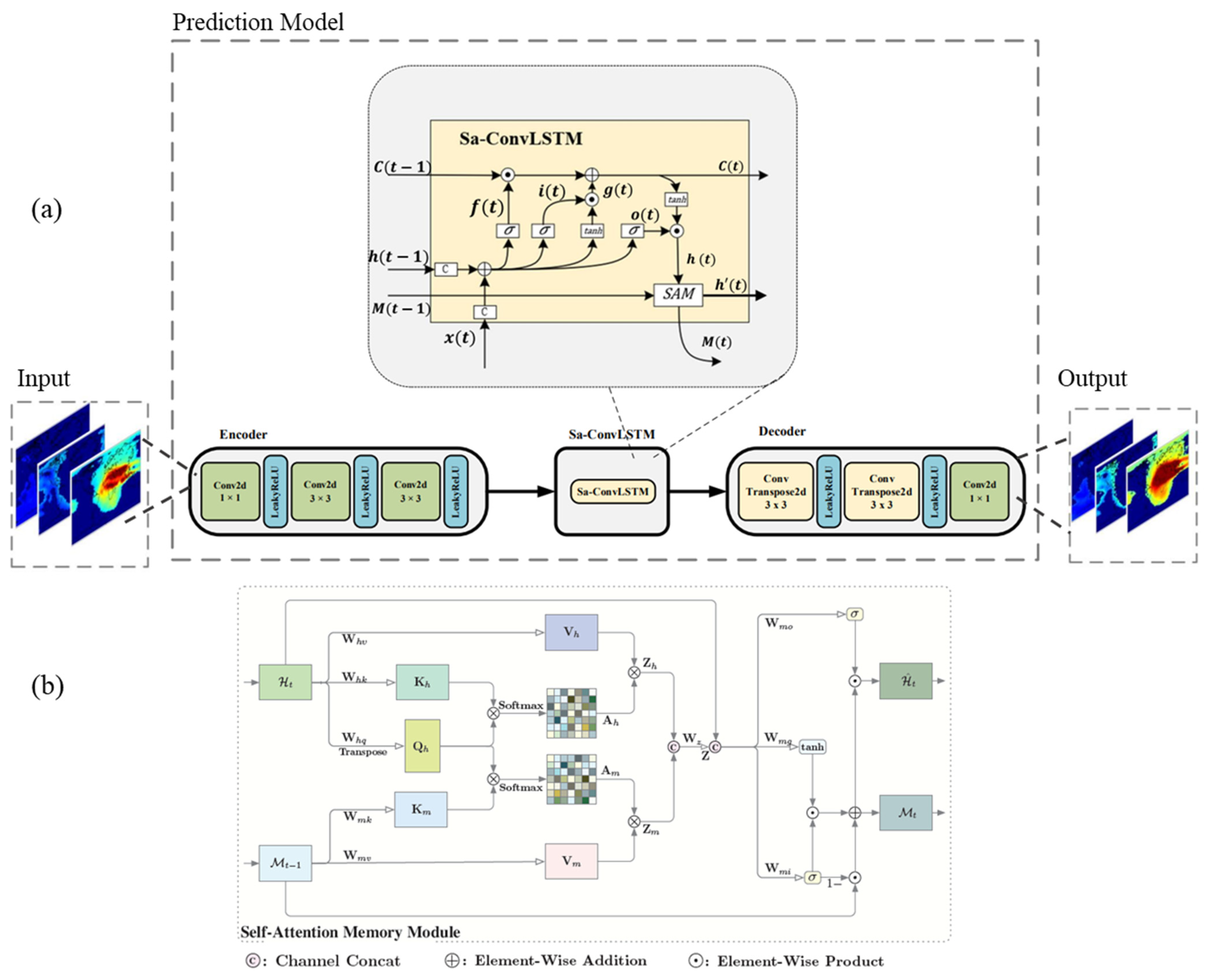
As mentioned above, the prediction of the TEC maps is very challenging due to the dynamic nature of the ionosphere. The ConvLSTM cell [20] can memorize the spatial characteristics of the TEC maps by utilizing convolution layers. We used SA-ConvLSTM [16] in this work because the global TEC variation has long-term spatial dependencies [21]. Figure 1a shows the structure of the SA-ConvLSTM cell and the self-attention memory (SAM) unit is detailed in Figure 1b. According to Figure 1a, the inputs to the module are c(t−1) (memory unit of the previous time), h(t−1) (hidden state of the previous time), and x(t) (current input data). The f(t) in the module determines which information needs to be retained until the next moment, while o(t) is the output part calculated based on h(t−1) and x(t). The h(t) is calculated by the SAM module and the h(t−1). According to Figure 1b, SAM accepts h(t) and memory of the previous step M(t−1). The self-attention mechanism is used to extract the global dependency of inputs. For example, in the field of machine translation, the temporal correlation can be extracted, and in the field of image recognition, the spatial correlation can be extracted [22,23]. SAM calculates the similarity between h(t) and M(t−1), and based on the results, obtains new M(t) and h′(t) (input to the next hidden state).
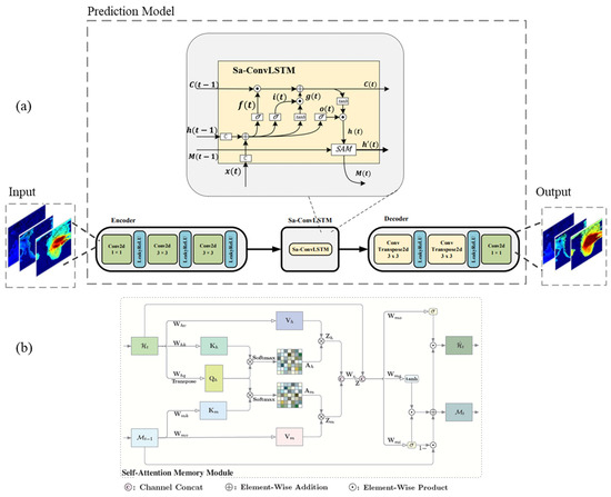
Figure 1.
(a) Structure of the model. The model consists of three parts, which are encoder, SA-Convlstm unit, and decoder. (b) Structure of the self-attention memory (SAM).
However, if all ConvLSTM cells in the model proposed by Liu et al. [14] are updated to SA-ConvLSTM cells, it will greatly increase the complexity of the model. Thus, we used a convolutional encoder–decoder architecture [17] to encode and compress the TEC maps.
The hyperparameters and the image size after passing through each layer of the encoder and decoder are presented in Table 1. The Random Search method for hyperparameter optimization proposed by Bergstra and Bengio [24] was adopted to choose the optimal hyperparameters. During the experiment, we set 5 groups of alternative values for the three hyperparameters of Batch size, Learning rate, and Epoch, and searched with the RandomSearch method to finally select the parameter values in Table 1.The number of the parameters of the entire model is 605,570 which is 30 percent smaller than the model (915,282) in Liu’s work [14].

Table 1.
Model parameters and the input and output size of each layer.
2.2. Dataset and Processing
The global ionospheric total electron content (TEC) maps have been generated by International GNSS Service (IGS) since 1998. For this study, we utilized the GIM provided by the Centre for Orbit Determination in Europe (CODE) (URL). The GIM data are generated by spherical harmonic filling, ensuring that there are no missing data points on each map. The temporal resolution of the CODE global ionospheric map (GIM) is 1 h, with longitude ranging from 180°W to 180°E and a spatial resolution of 5°, and latitude ranging from 87.5°N to 87.5°S with a spatial resolution of 2.5°. The resulting TEC map has the dimensions of 71 × 73 = 5183 grid points.
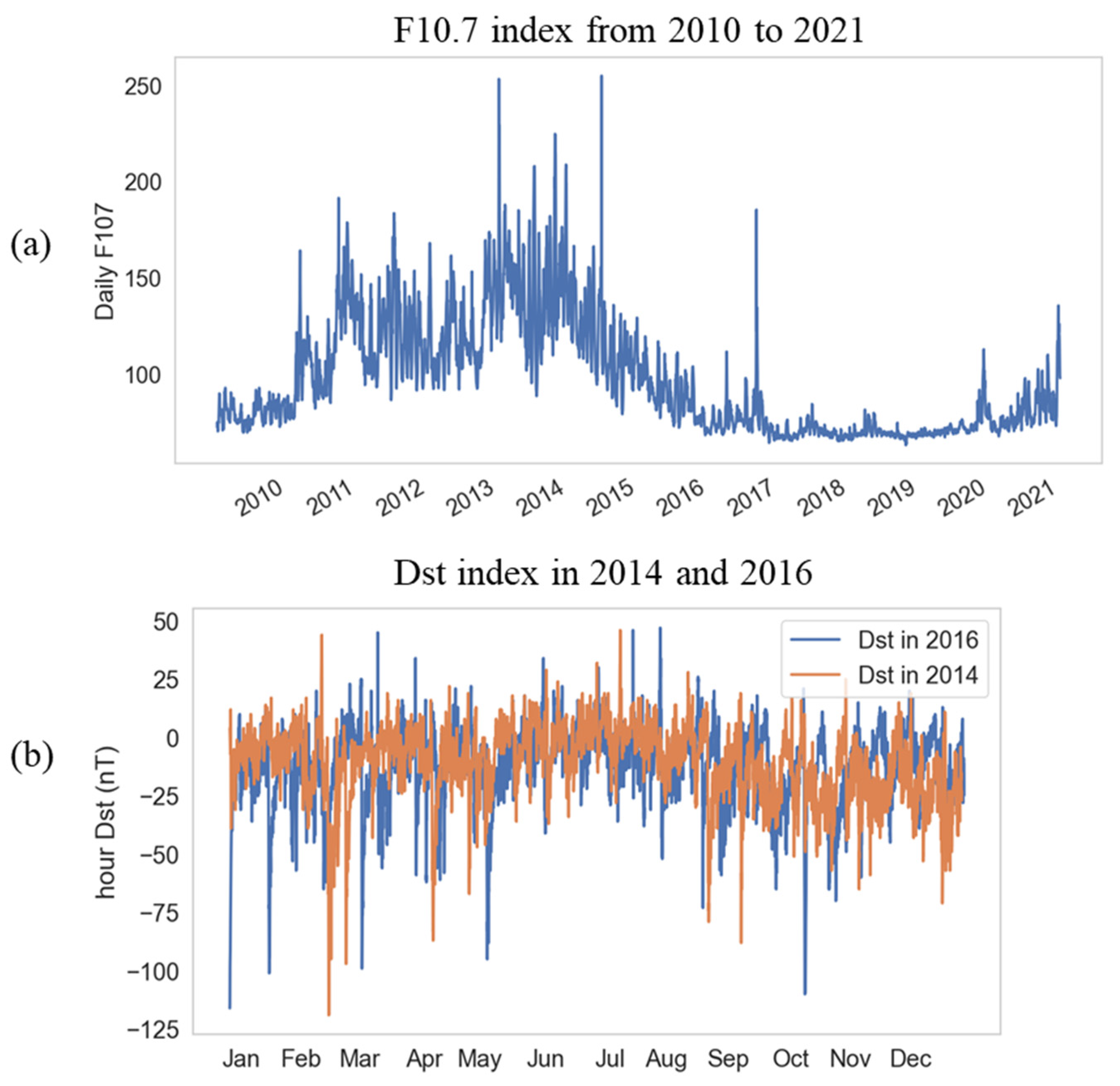
The total electron content (TEC) varies with solar and geomagnetic activities [25,26,27]. To indicate the activity levels, we used the F10.7 and Dst indexes, with the specific criteria shown in Table 2. Figure 2a illustrates the F10.7 index variation from 2011 to 2021, indicating 2016 as a low solar activity year and 2014 as a high solar activity year. Figure 2b displays the Dst index variation in 2014 and 2016. We tested the predictive performance of the model using data from magnetic storms and geomagnetic quiet periods during the high solar activity year (2014) and low solar activity year (2016). For the 2014 test, we trained using data from 2011 to 2013, and for the 2016 test, we uses data from 2013 to 2015; we hope to use data from the past three years for training to predict the results of the next year. The training set accounted for 80%, and the test set accounted for 20%.
Table 2.
Classification of solar and geomagnetic activity levels.
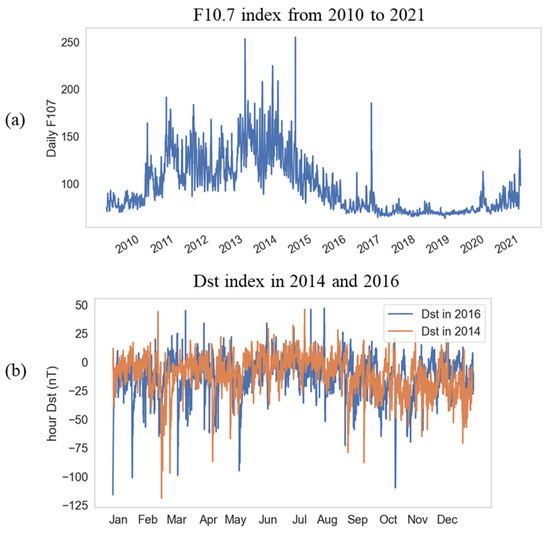
Figure 2.
(a) F10.7 index showing the solar activity from 2010 to 2011. (b) The Dst index is used to describe the geomagnetic activity in 2014 and 2016.
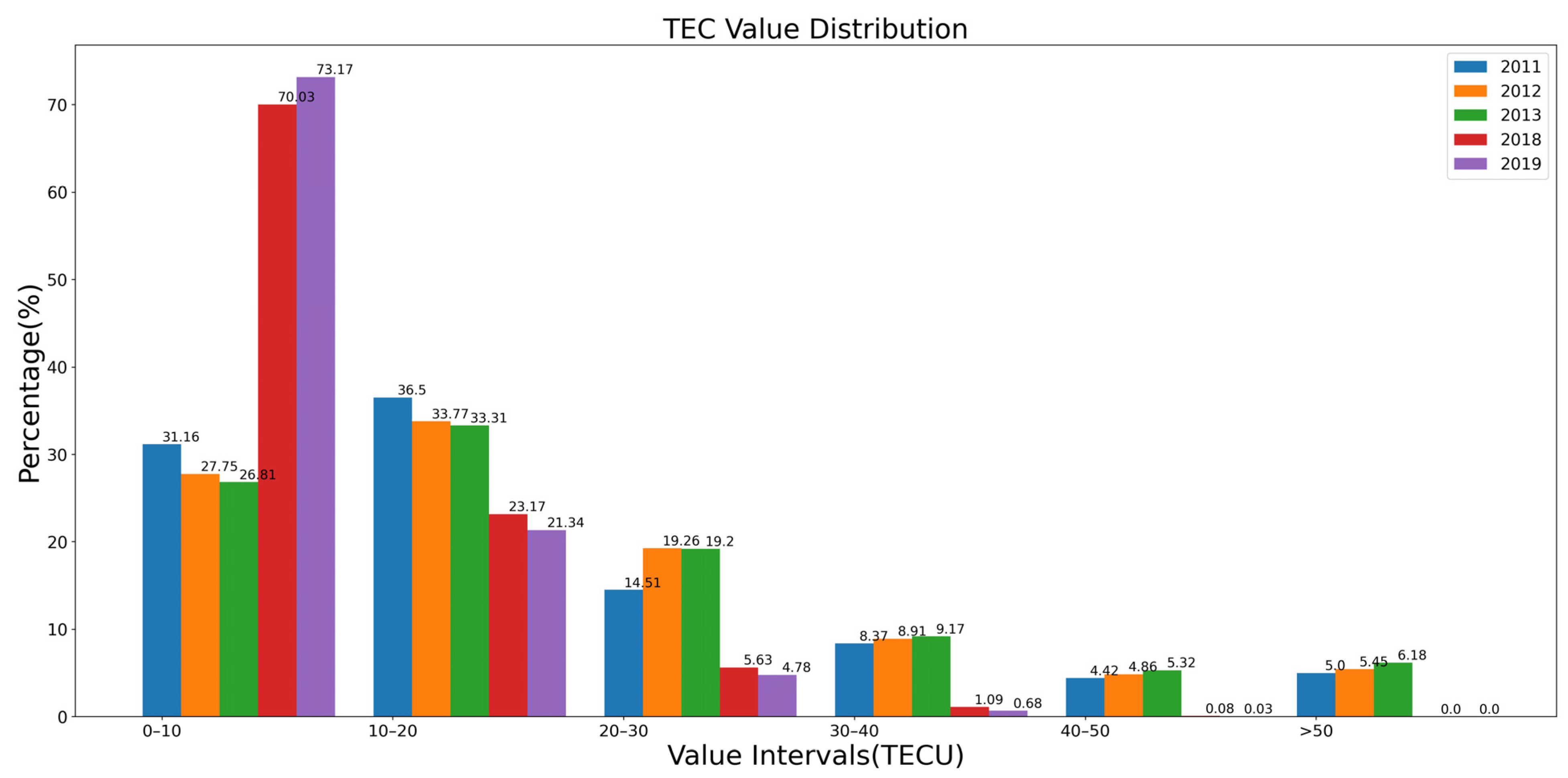
Although the global TEC map is highly complex in both the spatial and temporal dimensions, it also exhibits certain patterns. Guo et al. [19] studied the distribution of global TEC from 1999 to 2013 and found a gradual decrease from low to high latitudes, with anomalies occurring at the equatorial crest and Greenland. In order to avoid introducing prior information into the test set, we calculated the global TEC value distribution range in 2011, 2012, 2013, 2018, and 2019, and the results are shown in Figure 3. The first three years represent the distribution of TEC in high solar activity years, and the last two years represent the distribution of TEC in low solar activity years. Statistical analysis revealed that the highest fraction of TEC values was between 0–10 TECU and 10–20 TECU, while the fraction of TEC values above 20 TECU was less than 50% in both low and high solar activity years. According to Guo et al. [19], regions with greater than 20 TECU are mainly concentrated in the middle and low latitudes on both sides of the equator. We used 10 TECU and 20 TECU as thresholds to divide the dataset into three parts: 0–10 TECU, 10–20 TECU, and greater than 20 TECU. When making predictions, we will make predictions for the three parts in the order of TEC size. After each part is predicted, a loss will be calculated once, and when the losses for all three parts are calculated, we will complete the prediction for one graph. After the three parts are predicted, we will sum the results of the three parts and output them. The ionosphere is often disturbed by sudden factors such as magnetic storms, which cause irregular variations of TEC [28,29,30]. Therefore, we shuffl Aggarwalle the data by day within a year to improve the model’s anti-disturbance ability. The results demonstrated that the overall accuracy of the model significantly improved after shuffling.
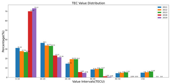
Figure 3.
The distribution of TEC values in different intervals for 2011, 2012, 2013, 2018 and 2019 were counted.
2.3. Evaluation Metrics
In this paper, ME (Mean Error), MSE (Mean Square Error), MAE (Mean Absolute Error), and RMSE (Root Mean Square Error) are used to verify the prediction performance of the model. The formulas of the above three metrics are as follows:
In the above formula, is the model’s predicted value of a point in the TEC map grid, is the true value of a point in the TEC map grid provided by IGS, and is the resolution size of the TEC map, which is .
3. Result and Discussion
3.1. Training and Test Result Analysis
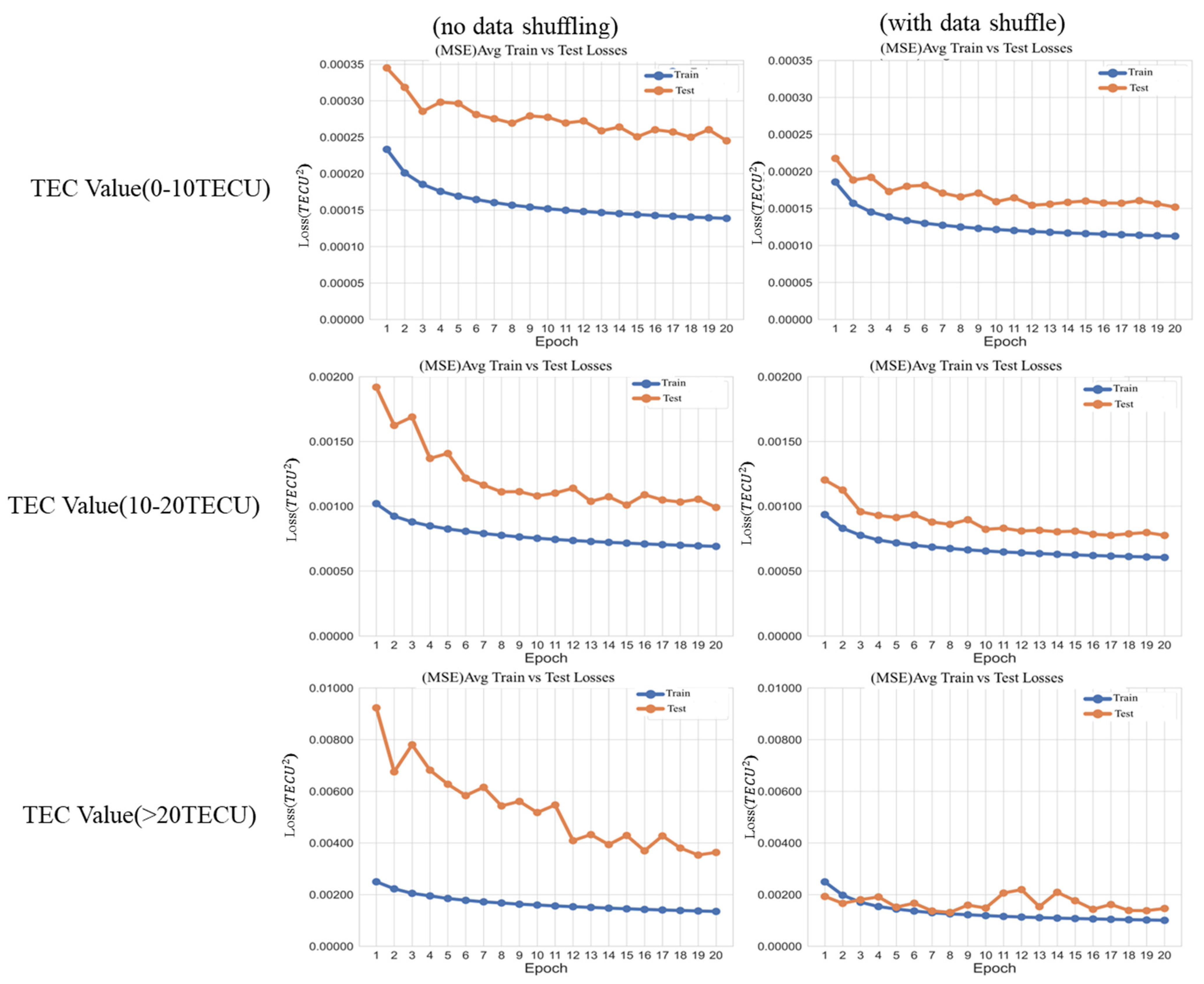
As described in Section 2, we utilized thresholds of 10 and 20 TECU to divide the TEC images into three groups. We also shuffled the data within each year based on the days. Figure 4 shows the training and test effect of the model with and without shuffling on the order of TEC maps. In the experiment, one epoch represents training all data once. Based on multiple experiments, we found that when epoch = 20, the model converges, so we set the number of epochs to 20.
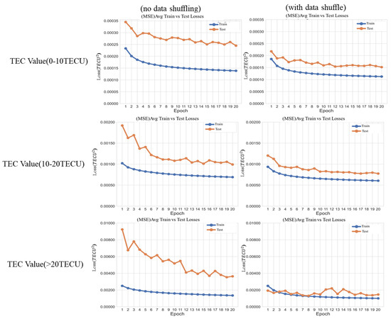
Figure 4.
The three plots on the left depict the training (2011–2013) and test (2014) effect of different groups without shuffling. The right plots show the training effects of different intervals under the shuffling.
The results show that both dataset processing methods can make the model prediction results converge, but the method of shuffling can improve the model prediction performance. Based on the results in Figure 4, we compared the average losses of the last four periods with and without shuffling. The calculation results show that after shuffling, the training errors of the three groups decreased by 21%, 3%, and 2%, respectively, but the testing errors decreased by 40%, 25%, and 53%, respectively. The reason for these results may be that the shuffling process is equivalent to artificially adding disturbances to the dataset and improving the robustness of the model. The performance is particularly improved in regions with TEC values greater than 20, most of which are located at low and mid-latitudes on both sides of the equator that the regions with the largest gradient of TEC. It shows [31] that the TEC daily variation has two distinct peaks, and the phenomenon is most pronounced in the equatorial region due to the largest TEC background values.
The TEC is affected by irregular disturbances, and it will change greatly during a magnetic storm. Therefore, shuffling the order of the data is beneficial to improve the robustness of the model during perturbation, especially in the equatorial region that has the most pronounced diurnal variation. It can also be seen from the results that the prediction error will increase with the increase in TEC value.
3.2. Low Solar Activity Years
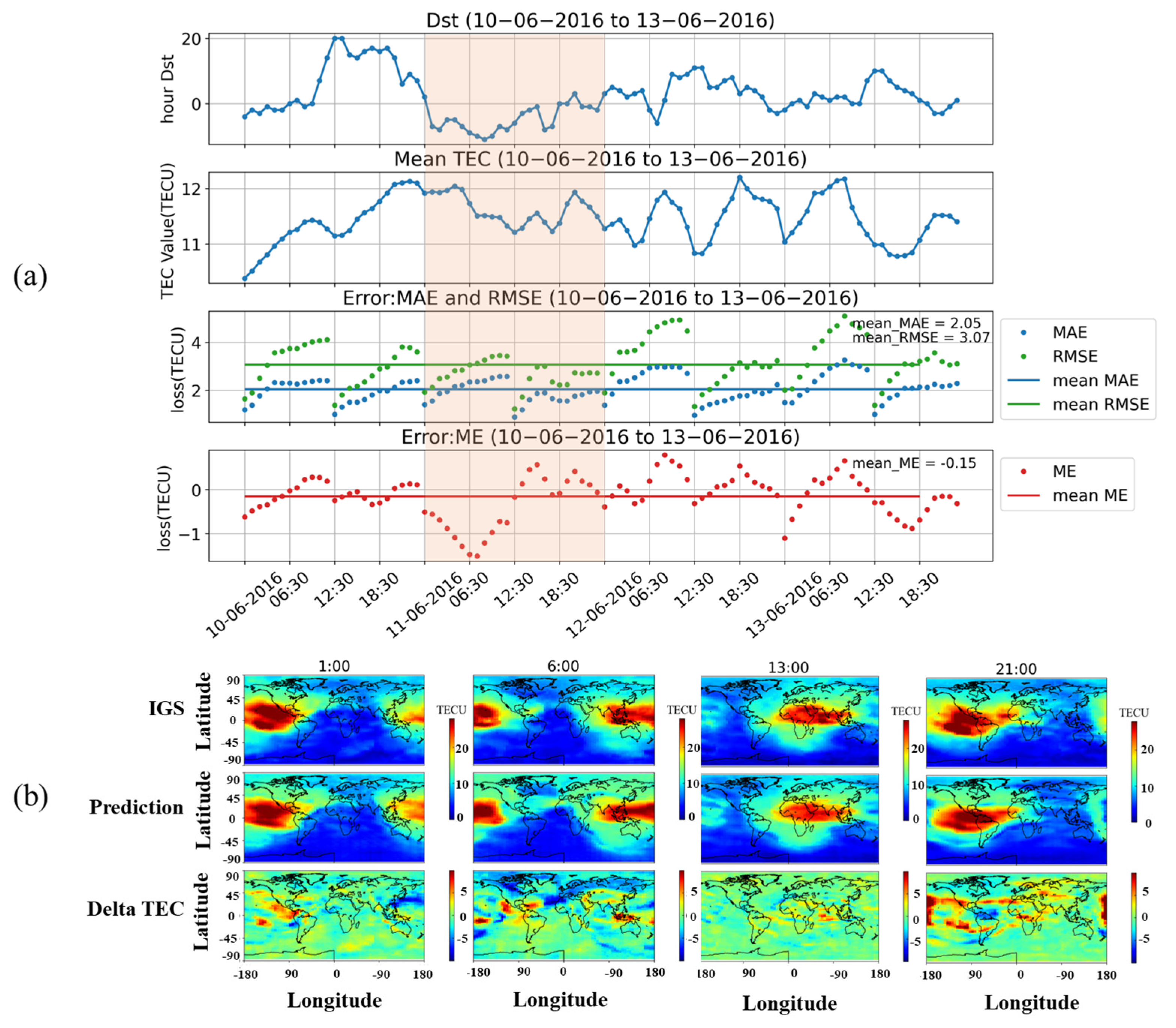
In this section, we present the model prediction results for 2016, which was a year of low solar activity. Specifically, we examine the model’s performance during both a geomagnetic quiet period and a magnetic storm. For our analysis, we selected 10–13 June 2016 as the testing period, during which we assessed the model’s prediction accuracy under low solar activity conditions. Figure 5a illustrates the Dst index (top), global TEC means (second panel), RMSE, MAE (third panel), and ME (bottom) over the four-day period. The solid lines in green, blue, and red represent the mean values of RMSE, MAE, and ME, respectively, which were calculated using the expression described in Section 2.3. The resulting values for the four days were 3.07, 2.05, and −0.15, respectively. To provide a more detailed view of the model’s performance, we extracted the results during the highlighted interval in Figure 5a and present them in Figure 5b. The results in Figure 5b correspond to 11 June 2016, at 1:00 UT, 6:00 UT, 13:00 UT, and 21:00 UT, from left to right, respectively. From top to bottom, Figure 5b shows the actual TEC data provided by IGS, the model’s predicted results, and the error Delta TEC, which represents the residuals between the actual and predicted data. The formula for calculating Delta TEC is shown below.

Figure 5.
(a) Dst index, global TEC means, RMSE, MAE, and ME from 10 to 11 June 2016. The green line and blue line in the third figure show the mean RMSE and MAE during this period. The red line in the fourth figure shows the mean ME. (b) Real TEC data released by IGS, prediction result, and delta TEC during the time interval framed by the red transparent box in (a).
Since the experiment was predicted with a 12 h time interval, the first predicted results by the model were at 1:00 and 13:00. Analysis of the results reveals that the model’s prediction accuracy decreases with an increase in the prediction time step. Furthermore, we also observed that the model can predict the structure of the graph accuracy, particularly the equatorial ionization anomaly (EIA) [32] phenomenon.
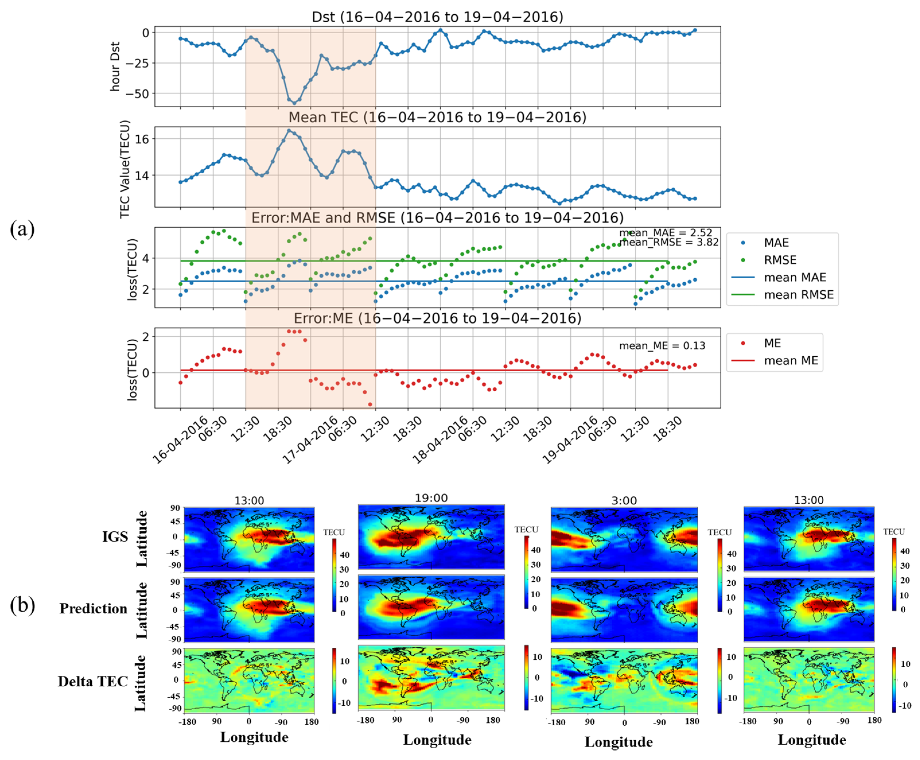
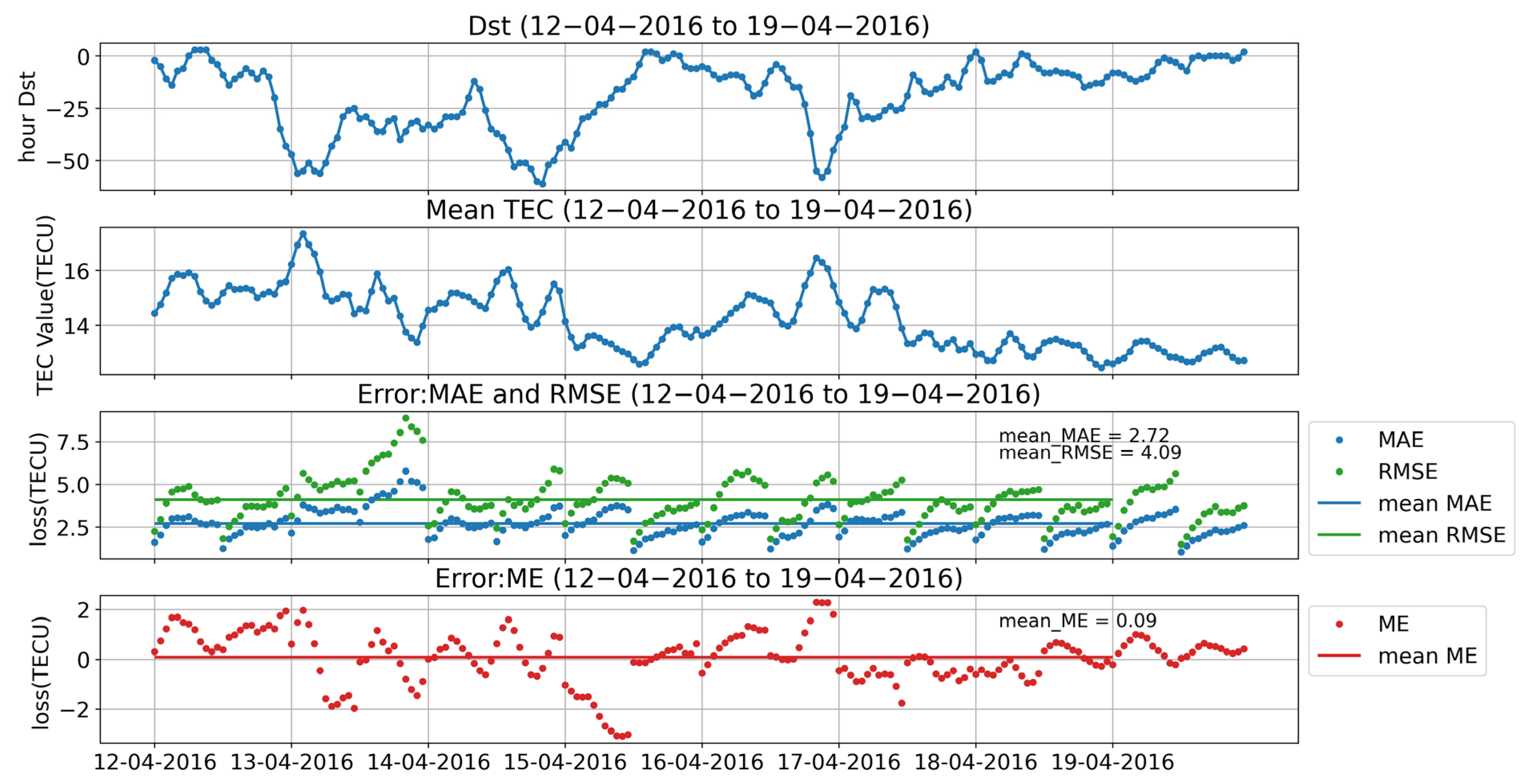
To assess the model’s prediction accuracy during a magnetic storm, we selected the period from 16 to 19 April 2016, which covers the initial, main, and recovery phases of the storm. During this period, the Dst index reached a minimum of −60 nT, and the structure of Figure 6a was similar to that of Figure 5a. The mean values of RMSE, MAE, and ME for the selected period were 3.82, 2.52, and 0.13, respectively. The highlighted boxes in Figure 6a represent the time intervals for which Figure 6b presents the corresponding results. Specifically, the results in Figure 6b correspond to 16 April 2016 at 13:00 UT (initial phase of the magnetic storm) and 19:00 UT (main phase), and 17 April 2016 at 13:00 UT (main phase) and 21:00 UT (recovery phase).
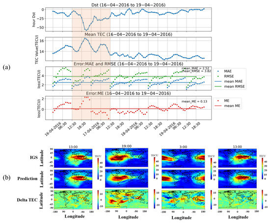
Figure 6.
(a) Dst index, global TEC means, RMSE, MAE, and ME from 16 to 19 April 2016. The green line and blue line in the third figure show the mean RMSE and MAE during this period. The red line in the fourth figure shows the mean ME. (b) Real TEC data released by IGS, prediction result, and delta TEC during the time interval framed by the red transparent box in (a).
Compared to the average error of the model during the geomagnetic quiet period, there was a significant increase in prediction error at middle and low latitudes during the magnetic storm period. However, the model’s ability to predict the structure of the TEC map remained relatively accurate. Notably, the model’s prediction accuracy was lower during the main phase of the magnetic storm compared to the initial and recovery phases. The errors were predominantly concentrated at middle and low latitudes.
3.3. High Solar Activity Years
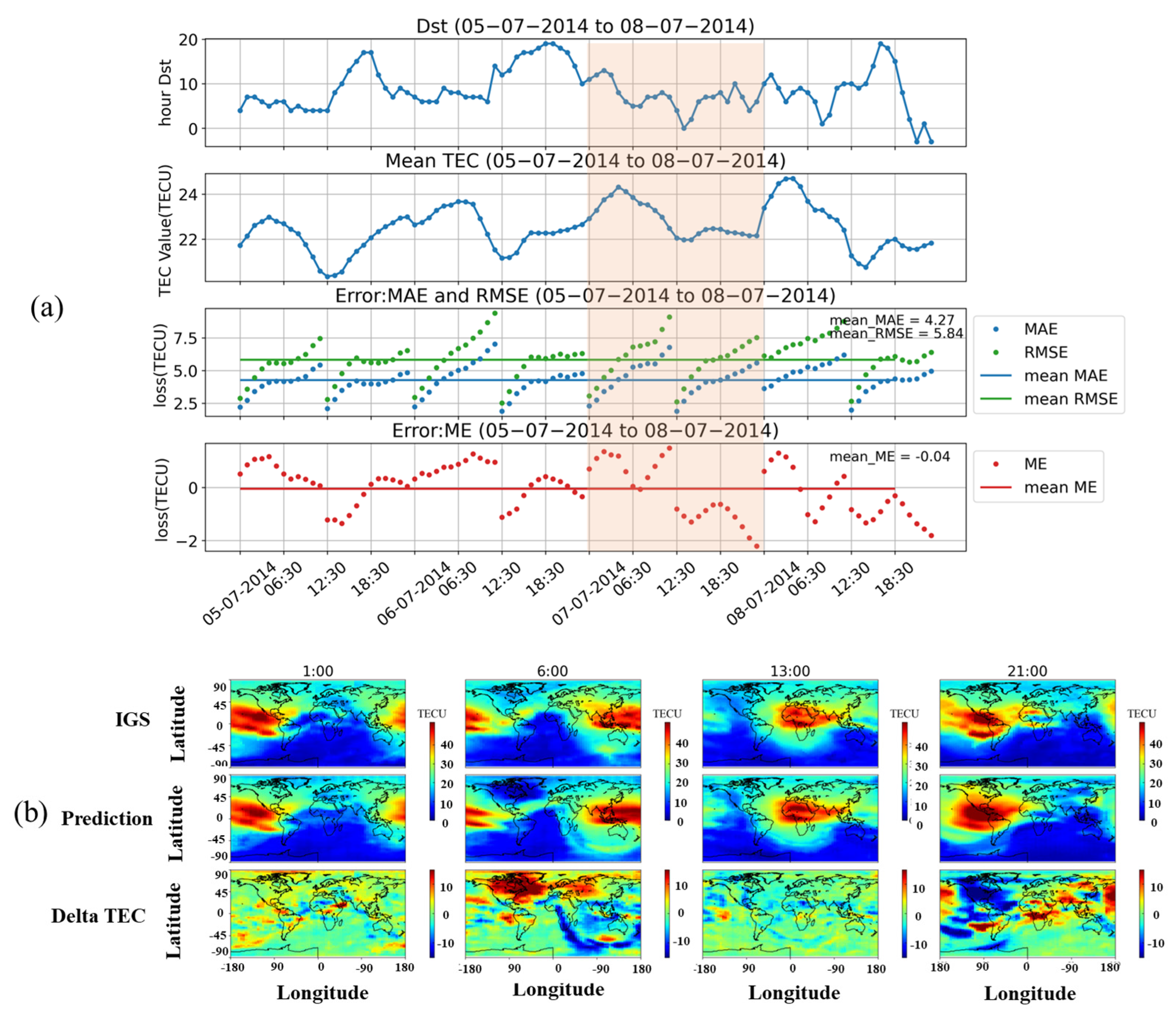
In this section, we selected the period from 5 to 8 July 2014, to test the prediction performance of the model during geomagnetic quiet and high solar activity conditions. Figure 7a indicates that the average global TEC in 2014 was roughly double that in 2016. The average RMSE, MAE, and ME values during these four days were 5.84, 4.27, and −0.04, respectively. The results in Figure 7b represent 1:00 UT, 6:00 UT, 13:00 UT, and 21:00 UT on 7 July 2014, respectively. From the results, it can be observed that RMSE and MAE were larger in 2014 than in 2016, while ME was smaller than in 2014. As shown in Figure 8a, during the magnetic storm period from 12 to 16 September 2014, the average values of RMSE, MAE, and ME were 5.96, 4.19, and 0.28, respectively. During this period, the minimum Dst was less than −75nT, and the disturbance intensity was higher than in 2014.

Figure 7.
(a) Dst index, global TEC means, RMSE, MAE, and ME from 5 to 8 July 2014. The green line and blue line in the third figure show the mean RMSE and MAE during this period. The red line in the fourth figure shows the mean ME. (b) Real TEC data released by IGS, prediction result, and delta TEC during the time interval framed by the red transparent box in (a).
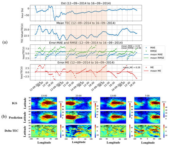
Figure 8.
(a) Dst index, global TEC means, RMSE, MAE, and ME from 12 to 16 September 2014. The green line and blue line in the third figure show the mean RMSE and MAE during this period. The red line in the fourth figure shows the mean ME. (b) Real TEC data released by IGS, prediction result, and delta TEC during the time interval framed by the red transparent box in (a).
The times of the results in Figure 8b are 12 September 2014 at 13:00 UT (initial phase of the magnetic storm) and 23:00 UT (main phase), 13 September at 13:00 UT (recovery phase), and 14 September at 7:00 UT (recovery phase). From the results, the prediction results of the model during the main phase were different from those of the initial phase and recovery. The forecast error was similar to that of the 2016 geomagnetic quiet period but larger than that of the 2016 magnetic storm.
3.4. Comparison and Analysis of Testing Results
Table 3 presents a comparison between the maximum and minimum daily average forecast errors of our model and Liu’s model. Figure 7 and Figure 8 of Liu’s paper are statistical results, so we also compared the results of our Figure 5, Figure 6, Figure 7 and Figure 8 with Liu’s results after statistical analysis. Our analysis covers both calm periods and major phases of magnetic storms during years of high and low solar activity. Since Liu’s paper did not provide a specific date for the prediction results, we conducted a comparison using the results of magnetic storms and geomagnetic quiet periods in years of low solar activity to compare with Liu’s results for the same period. The same approach was used for years of high solar activity. Specifically, we compared the results of our model for magnetic storm periods during low and high solar activity years with Liu’s results for magnetic storm periods, and the same procedure was applied for calm periods. The statistical average time refers to the period corresponding to Figure 5, Figure 6, Figure 7 and Figure 8. By using this method, we were able to effectively compare the performance of our model with Liu’s model for different phases of solar activity.
Table 3.
Model prediction error during testing.
In Table 3, our model achieved a lower minimum error value than Liu’s, and the majority of the maximum error values were within 2 TECU. These findings suggest that our model’s prediction accuracy is comparable to that of Liu’s model.
For the convenience of comparison, Figure 9 shows the results for the same period as Figure 6 in Liu et al. [14]. Table 4 presents the ME and RMSE values for our model, Liu’s model, and the 1-day predicted global TEC products released by the CODE analysis center (c1pg) for the same time period.
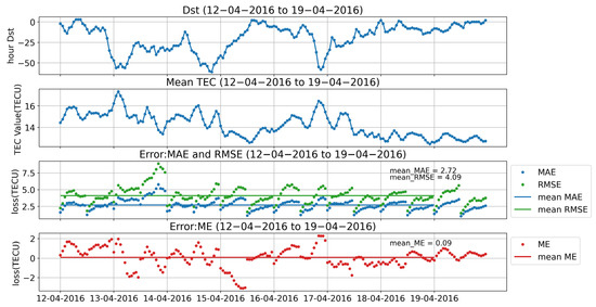
Figure 9.
Predictive results for the magnetic storm events from 12 to 19 April 2016.
Table 4.
Comparison of the predictive ability of three models for the magnetic storm events from 12 to 19 April 2016.
In Table 4, the average MSE of our predicted results was 0.09, slightly lower than Liu et al.’s [14] result of −0.14 and c1pg’s result of −0.44. The average RMSE of our predicted results was 4.09, slightly higher than Liu et al.’s [14] result of 2.52 and c1pg’s result of 3.12. The sum of the parameters for our entire model was 605,570, which is 30% smaller than that of Liu’s model (915,282). Overall, our model’s accuracy can be compared to the above models, but with reduced complexity, while maintaining accuracy, achieving the intended purpose of this work.
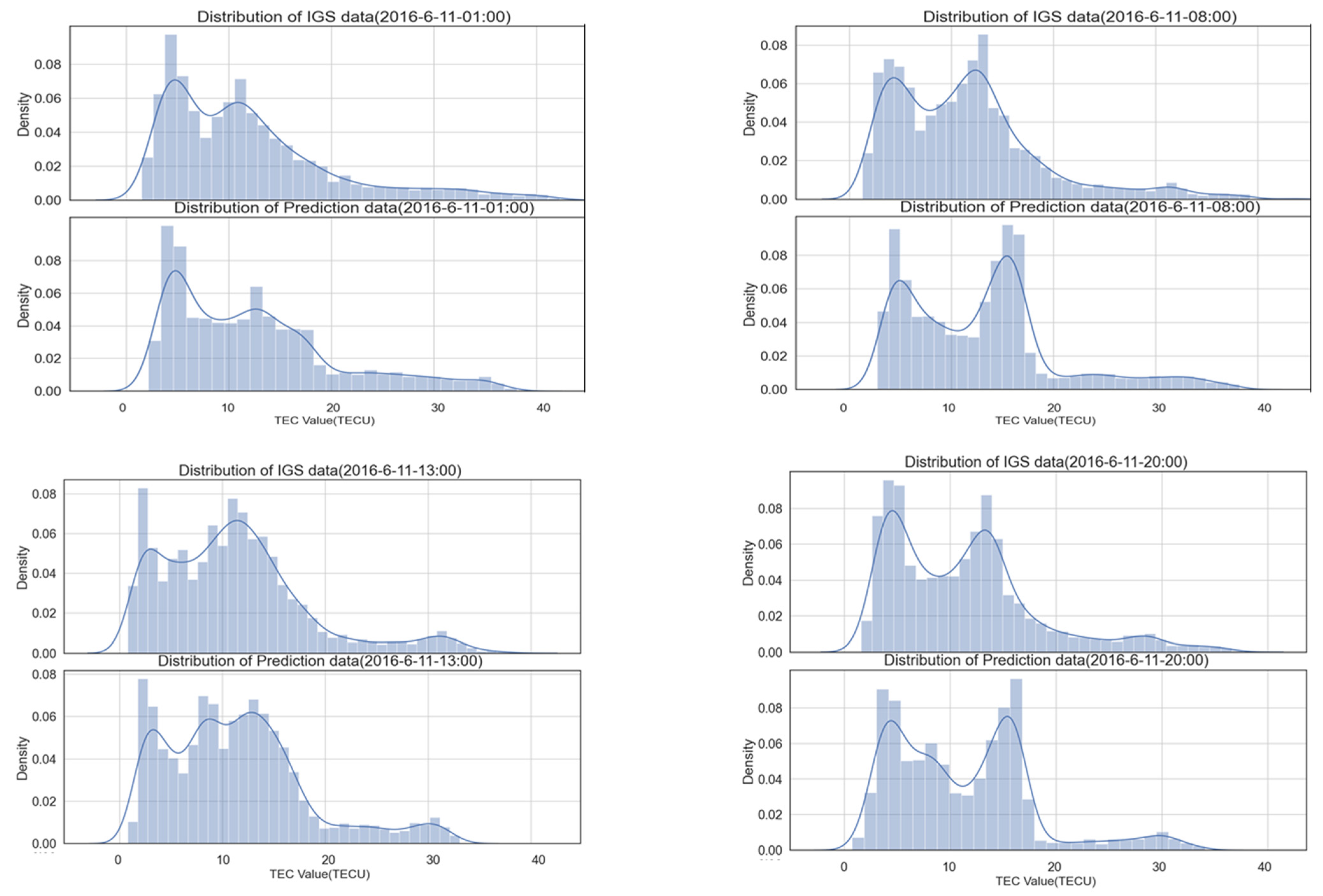
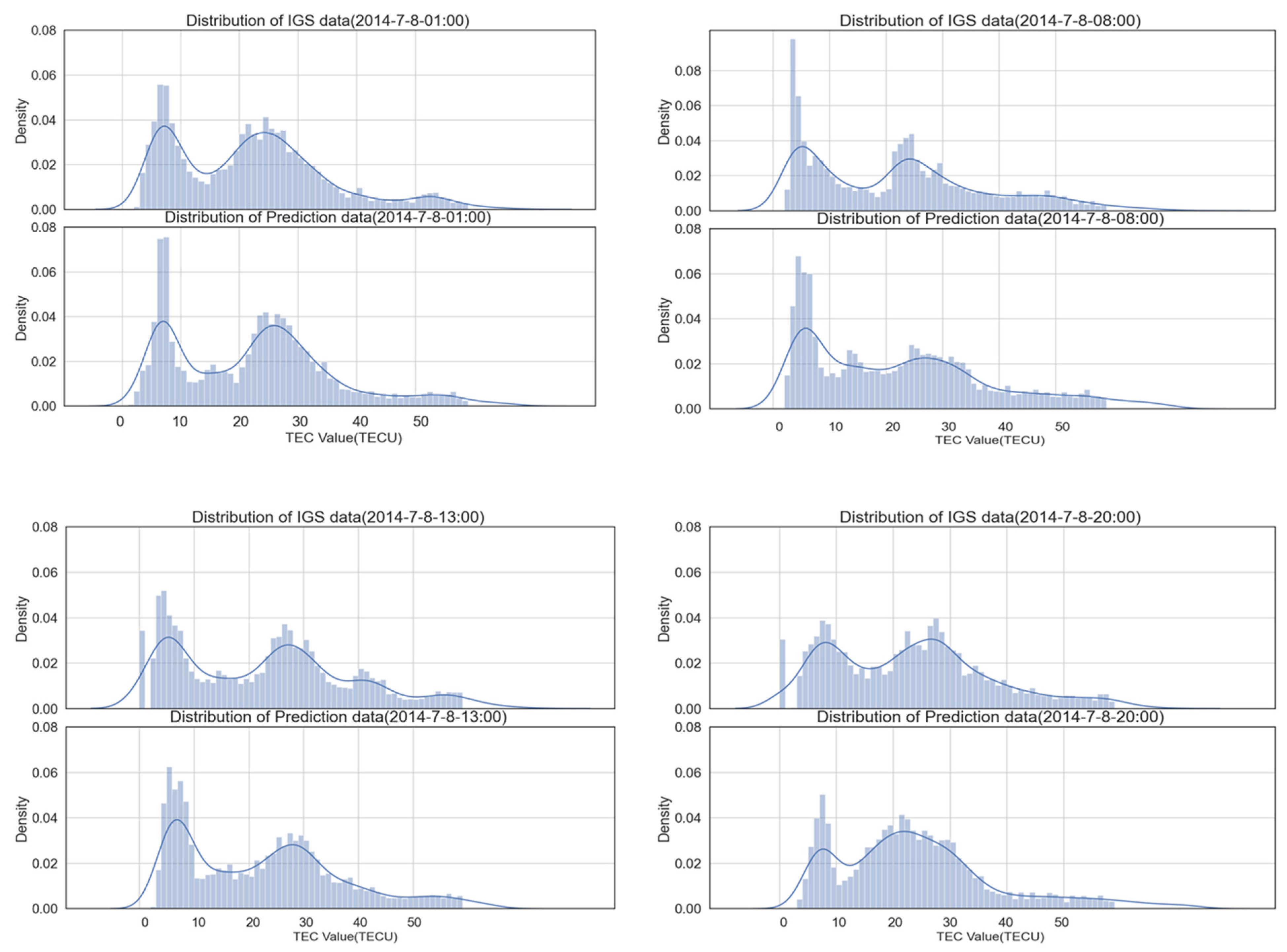
Figure 10 and Figure 11 show the quantitative distribution of the predicted results and actual TEC values. Figure 10 displays the distribution of predicted and actual data at 1:00, 6:00, 13:00, and 20:00 on 11 June 2016, while Figure 11 shows the distribution on 7 July 2014, at the same times. An analysis of Figure 10 reveals that the prediction errors were primarily concentrated around 10 TECU. On both sides of 10 TECU, the model’s prediction results showed good agreement with the actual TEC distribution. Similarly, an analysis of Figure 11 shows that the forecast results in 2014 were closer to the actual distribution than those in 2016. The forecast errors in 2014 were relatively concentrated around 25 TECU. The global TEC background value of that year was the annual average value of the global TEC. Based on an analysis of the distribution of prediction errors in 2014 and 2016 and the TEC background value in Figure 12, it can be concluded that the prediction errors are mainly concentrated near the background value.
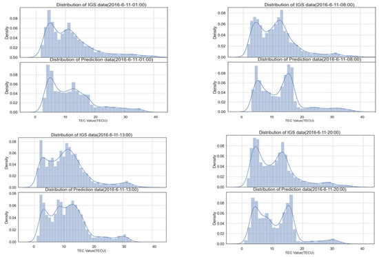
Figure 10.
Distribution of predicted results and the actual TEC distribution on 11 June 2016.
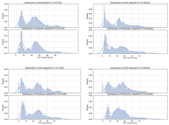
Figure 11.
Distribution of predicted results and the actual TEC distribution on 8 July 2014.
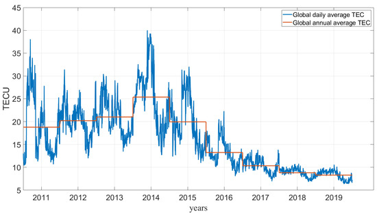
Figure 12.
Global daily average TEC (blue line) and global annual average TEC (red line) from 2011 to 2019.
4. Conclusions
This paper proposed a lightweight global TEC prediction model that achieves high precision. To achieve this goal, we introduced the SA-ConvLSTM unit, which improves a single prediction unit’s ability to extract long-distance spatiotemporal feature dependencies. Additionally, we introduced an encoder–decoder to compress data, extract features, and enhance prediction accuracy. We also applied a preprocessing method for the dataset, which divides each TEC map into three subgroups according to predefined thresholds to reduce data complexity. Furthermore, we shuffled the dataset sequence to improve its robustness, and the training curve showed that this process greatly improved the model’s accuracy. We made consecutive predictions during magnetic storms and geomagnetic lulls in both 2014 (a high solar activity year) and 2016 (a low solar activity year). The prediction results in 2016 were mainly concentrated around 10 TECU, and the results in 2014 were mainly concentrated around 25 TECU. Overall, the accuracy of the model’s prediction is mainly affected by the background value of the global TEC. The average global TEC during high solar activity years is almost twice that of low solar activity years, so the global average error during high solar activity years will be higher than that in low solar activity years. The model’s prediction performance decreases as the prediction time step increases. Nonetheless, the model shows good potential, and increasing the number of model layers can also improve the model’s accuracy.
Author Contributions
Conceptualization, H.C.; Methodology, X.Y.; Software, X.Y.; Investigation, C.X. and L.Y.; Writing—original draft, X.Y.; Writing—review & editing, H.C. and W.Z.; Visualization, X.Y.; Funding acquisition, H.C. All authors have read and agreed to the published version of the manuscript.
Funding
This work was jointed supported by the National Nature Science Foundation of China (42074185) and the Special Fund of Hubei Luojia Laboratory (No. 220100013).
Data Availability Statement
The global Total Electron Content map data used in this work were obtained from the Goddard Space Flight Center, space physics data facility (https://spdf.gsfc.nasa.gov/pub/data/gps/tec1hr_igs/, accessed on 31 December 2019). F107 index and Dst index can be obtained from the link https://omniweb.gsfc.nasa.gov/, accessed on 31 December 2021.
Conflicts of Interest
The authors declare no conflict of interest.
References
- McNamara, L.F. The Ionosphere: Communications, Surveillance, and Direction Finding; Krieger: Malabar, FL, USA, 1991. [Google Scholar]
- Kersley, L.; Malan, D.; Pryse, S.E.; Candetr, L.R.; Bamford, R.A.; Belehaki, A.; Leitinger, R.; Radicella, S.M.; Mitchell, C.N.; Spencer, P.S.J. Total electron content-A key parameterin propagation: Measurement and usein ionospheric imaging. Ann. Geophys. 2004, 47 (Suppl. S2–S3), 1067–1091. [Google Scholar] [CrossRef]
- Mannucci, A.J.; Wilson, B.D.; Yuan, D.N.; Ho, C.H.; Lindqwister, U.J.; Runge, T.F. A global mapping technique for GPS-derived ionospheric total electron content measurements. Radio Sci. 1998, 33, 565–582. [Google Scholar] [CrossRef]
- Bust, G.S.; Mitchell, C.N. History, current state, and future directions of ionospheric imaging. Rev. Geophys. 2008, 46. [Google Scholar] [CrossRef]
- Huba, J.D.; Joyce, G.; Fedder, J.A. Sami2 is Another Model of the Ionosphere (SAMI2): A new low-latitude ionosphere model. J. Geophys. Res. Space Phys. 2000, 105, 23035–23053. [Google Scholar] [CrossRef]
- Huba, J.; Krall, J. Modeling the plasmasphere with SAMI3. Geophys. Res. Lett. 2013, 40, 6–10. [Google Scholar] [CrossRef]
- Fesen, C.G.; Crowley, G.; Roble, R.G.; Richmond, A.D.; Fejer, B.G. Simulation of the pre-reversal enhancement in the low latitude vertical ion drifts. Geophys. Res. Lett. 2000, 27, 1851–1854. [Google Scholar] [CrossRef]
- Bilitza, D.; Pezzopane, M.; Truhlik, V.; Altadill, D.; Reinisch, B.W.; Pignalberi, A. The International Reference Ionosphere model: A review and description of an ionospheric benchmark. Rev. Geophys. 2022, 60, e2022RG000792. [Google Scholar] [CrossRef]
- Materassi, M. The Complex Ionosphere; Chapter 15 of this book; Elsevier Science: Amsterdam, The Netherlands, 2019. [Google Scholar] [CrossRef]
- Shim, J.S.; Kuznetsova, M.; Rastätter, L.; Hesse, M.; Bilitza, D.; Butala, M.; Codrescu, M.; Emery, B.; Foster, B.; Fuller-Rowell, T.; et al. CEDAR electrodynamics thermosphere ionosphere (ETI) challenge for systematic assessment of ionosphere/thermosphere models: NmF2, hmF2, and vertical drift using ground-based observations. Space Weather 2011, 9. [Google Scholar] [CrossRef]
- Liu, L.; Zou, S.; Yao, Y.; Wang, Z. Forecasting global ionospheric TEC using deep learning approach. Space Weather 2020, 18, e2020SW002501. [Google Scholar] [CrossRef]
- Chen, Z.; Liao, W.; Li, H.; Wang, J.; Deng, X.; Hong, S. Prediction of global ionospheric TEC based on deep learning. Space Weather 2022, 20, e2021SW002854. [Google Scholar] [CrossRef]
- Boulch, A.; Cherrier, N.; Castaings, T. Ionospheric activity prediction using convolutional recurrent neural networks. arXiv 2018, arXiv:1810.13273. [Google Scholar] [CrossRef]
- Liu, L.; Morton, Y.J.; Liu, Y. ML prediction of global ionospheric TEC maps. Space Weather 2022, 20, e2022SW003135. [Google Scholar] [CrossRef]
- Xia, G.; Zhang, F.; Wang, C.; Zhou, C. ED-ConvLSTM: A Novel Global Ionospheric Total Electron Content Medium-Term Forecast Model. Space Weather 2022, 20, e2021SW002959. [Google Scholar] [CrossRef]
- Lin, Z.; Li, M.; Zheng, Z.; Cheng, Y.; Yuan, C. Self-attention convlstm for spatiotemporal prediction. Proc. AAAI Conf. Artif. Intell. 2020, 34, 11531–11538. [Google Scholar] [CrossRef]
- Badrinarayanan, V.; Kendall, A.; Cipolla, R. Segnet: A deep convolutional encoder-decoder architecture for image segmentation. IEEE Trans. Pattern Anal. Mach. Intell. 2017, 39, 2481–2495. [Google Scholar] [CrossRef]
- Llewellyn, S.K.; Bent, R.B. Documentation and Description of the Bent Ionospheric Model; Rep. AFCRL-TR-73-0657; Air Force Geophys. Lab. Hanscom Air Force Base: Hanscom, MA, USA, 1973. [Google Scholar] [CrossRef]
- Guo, J.; Li, W.; Liu, X.; Kong, Q.; Zhao, C.; Guo, B. Temporal-spatial variation of global GPS-derived total electron content, 1999–2013. PLoS ONE 2015, 10, e0133378. [Google Scholar] [CrossRef]
- Shi, X.; Chen, Z.; Wang, H.; Yeung, D.-Y.; Wong, W.-K.; WOO, W.-C. Convolutional LSTM network: A machine learning approach for precipitation nowcasting. Adv. Neural Inf. Process. Syst. 2015, 28. [Google Scholar] [CrossRef]
- Calabia, A.; Jin, S. New modes and mechanisms of long-term ionospheric TEC variations from global ionosphere maps. J. Geophys. Res. Space Phys. 2020, 125, e2019JA027703. [Google Scholar] [CrossRef]
- Vaswani, A.; Shazeer, N.; Parmar, N.; Uszkoreit, J.; Jones, L.; Gomez, A.N.; Kaiser, Ł.; Polosukhin, I. Attention is all you need. Adv. Neural Inf. Process. Syst. 2017, 30. Available online: https://papers.nips.cc/paper_files/paper/2017/hash/3f5ee243547dee91fbd053c1c4a845aa-Abstract.html (accessed on 25 July 2023).
- Hu, J.; Shen, L.; Sun, G. Squeeze-and-excitation networks. In Proceedings of the IEEE conference on computer vision and pattern recognition, Salt Lake City, UT, USA, 18–23 June 2018; pp. 7132–7141. [Google Scholar] [CrossRef]
- Bergstra, J.; Bengio, Y. Random Search for Hyper-Parameter Optimization. J. Mach. Learn. Res. 2012, 13, 281–305. Available online: https://dl.acm.org/doi/10.5555/2188385.2188395 (accessed on 22 August 2023).
- Bauer, S.J. Physics of Planetary Ionospheres; Springer Science & Business Media: Berlin/Heidelberg, Germany, 2012. [Google Scholar] [CrossRef]
- Knipp, D.J.; McQuade, M.K.; Kirkpatrick, D. Understanding Space Weather and the Physics Behind It; Learning Solutions; McGraw-Hill: New York, NY, USA, 2011. [Google Scholar] [CrossRef]
- Tapping, K.F. The 10.7 cm solar radio flux (F10.7). Space Weather 2013, 11, 394–406. [Google Scholar] [CrossRef]
- Essex, E.A.; Mendillo, M.; Schödel, J.P.; Klobuchar, J.; da Rosa, A.; Yeh, K.; Fritz, R.; Hibberd, F.; Kersley, L.; Koster, J.; et al. A global response of the total electron content of the ionosphere to the magnetic storm of 17 and 18 June 1972. J. Atmos. Terr. Phys. 1981, 43, 293–306. [Google Scholar] [CrossRef]
- Dashora, N.; Sharma, S.; Dabas, R.S.; Alex, S.; Pandey, R. Large enhancements in low latitude total electron content during 15 May 2005 geomagnetic storm in Indian zone. Ann. Geophys. 2009, 27, 1803–1820. [Google Scholar] [CrossRef]
- Chakraborty, M.; Kumar, S.; De, B.K.; Guha, A. Effects of geomagnetic storm on low latitude ionospheric total electron content: A case study from Indian sector. J. Earth Syst. Sci. 2015, 124, 1115–1126. [Google Scholar] [CrossRef]
- Aggarwal, M. TEC variability near northern EIA crest and comparison with IRI model. Adv. Space Res. 2011, 48, 1221–1231. [Google Scholar] [CrossRef]
- Balan, N.; Liu, L.B.; Le, H.J. A brief review of equatorial ionization anomaly and ionospheric irregularities. Earth Planet. Phys. 2018, 2, 257–275. [Google Scholar] [CrossRef]


Disclaimer/Publisher’s Note: The statements, opinions and data contained in all publications are solely those of the individual author(s) and contributor(s) and not of MDPI and/or the editor(s). MDPI and/or the editor(s) disclaim responsibility for any injury to people or property resulting from any ideas, methods, instructions or products referred to in the content. |
© 2023 by the authors. Licensee MDPI, Basel, Switzerland. This article is an open access article distributed under the terms and conditions of the Creative Commons Attribution (CC BY) license (https://creativecommons.org/licenses/by/4.0/).