SatelliteCloudGenerator: Controllable Cloud and Shadow Synthesis for Multi-Spectral Optical Satellite Images

Abstract

Optical satellite images of Earth frequently contain cloud cover and shadows. This requires processing pipelines to recognize the presence, location, and features of the cloud-affected regions. Models that make predictions about the ground behind the clouds face the challenge of lacking ground truth information, i.e., the exact state of Earth’s surface. Currently, the solution to that is to either (i) create pairs from samples acquired at different times or (ii) simulate cloudy data based on a clear acquisition. This work follows the second approach and proposes an open-source simulation tool capable of generating a diverse and unlimited number of high-quality simulated pair data with controllable parameters to adjust cloud appearance, with no annotation cost. The tool is available as open-source. An indication of the quality and utility of the generated clouds is demonstrated by the models for cloud detection and cloud removal trained exclusively on simulated data, which approach the performance of their equivalents trained on real data.

1. Introduction

Clouds are reported to affect a significant fraction of all acquired satellite imagery, with estimates as high as 55% over land and 72% over ocean [1]. For many downstream applications, such as land and crop monitoring, this type of obstruction can have a severe impact on the performance or altogether feasibility of a system. A significant amount of research [2,3,4,5,6,7,8,9] has been carried out on the topic of understanding clouds in satellite imagery as well as attempts to remove them.

The need for paired cloudy–clear image samples is particularly prominent in the context of cloud removal. This need is present in both key aspects of the design pipeline, namely, training and evaluation. At the training stage, it is often necessary to access a clear-sky sample and use it as ground truth to compute a loss for optimization. For paired image-translation frameworks, this ground truth should ideally correspond precisely to the input cloudy sample. At the evaluation stage, access to ground truth data pairs is also crucial, as computing a similar loss at inference is one of the key sources of information about the model’s performance.

There are currently two approaches for obtaining paired cloudy data (a corresponding pair of cloudy and cloud-free representations of the same image) explored in the literature. These include (i) the acquisition of temporally proximate real samples (achieving merely an approximation of the ground truth, with variable and hard-to-quantify precision) and (ii) the simulation of clouds based on a real source image with no clouds present (with precise ground truth).

This manuscript describes a new tool for simulating an unlimited number of diverse pairs of clear-sky and cloudy examples, following the second approach. The tool offers the capability to parameterize and control various features of the generated clouds.

The contributions of this work are as follows:

• It proposes a framework to generate synthetic clouds for satellite imagery, with adjustable parameters to synthesise diverse cloud types.
• It demonstrates that a cloud detection model trained solely on simulated data can approach the performance of a model trained on real data.
• Similarly, it demonstrates that a cloud removal model trained exclusively on simulated data can approach the performance of a model trained on real data.
• It demonstrates and highlights the advantages and disadvantages of synthetic and real paired cloudy data and it shows the different kinds of insight each data source can offer when evaluating cloud detection and cloud removal techniques.

Furthermore, the tool proposed in this work is openly shared on GitHub at https://github.com/strath-ai/SatelliteCloudGenerator (accessed on 22 August 2023), allowing for fast and easy incorporation into PyTorch-based deep learning schemes as an augmentation operation (it can process batches of stacked tensor input directly on GPU), as well as for evaluation.

The tool can be used for developing new methods for cloud detection and cloud removal but also beyond that, where it could be used as an augmentation type for tasks that deal with the risk of cloud presence, such as multi-sensor fusion, multi-temporal fusion, satellite image segmentation, object detection, or change detection.

2. Related Work

There are at least two distinct paths to achieving paired cloudy samples explored in the literature. Both approaches are motivated by the following limitation of the real physical world, namely, that it is most likely not physically possible to acquire a clear-sky observation and a corresponding cloudy observation, where all factors (such as lighting, exact time, or exact conditions on the planet’s surface), apart from the presence of the cloud, are kept constant.

The first approach to generating paired cloudy data relaxes this requirement for constant factors and it links cloudy and clear-sky images that are proximate in time. This occurs under the assumption that all other factors remain similar, rather than constant, within some feasible margin. However, the assumption may be too optimistic, and the conditions may vary enough to make the clear-sky sample an inaccurate approximation of the cloudy image with clouds removed. This is shown in Figure 1 with a sample from a commonly used SEN12MS-CR dataset [6]. To highlight the resulting changes better, two crops from the original pair are shown in greater detail. The selected regions of considerable change are indicated using the colored circles. As a result, inaccurate ground truth samples could be used for evaluation or learning if this approach is followed.

This approach has been explored in works such as [2,3,4,5,6,7]. In [2] and [5], Landsat image pairs are gathered with a time gap of 16 or 32 days. In [3], this gap is up to 15 days apart, while in [4] it could be up to 35 days. These lengths between acquired paired samples mean that the changes in the ground surface view may be profound even without any clouds present in either image. In the SEN12MS-CR dataset, it is ensured that the optical cloudy and cloud-free images are captured within the same meteorological season, which appears to be a rather loose constraint, as demonstrated in Figure 1. In the related work on the SEN12MS-CR-TS dataset [7], 30 samples evenly spaced in time are captured for each ROI across the full year, leading to temporal gaps of about 12 days.

The alternative approach maintains the constant-factor requirement by simulating the cloud component and adding it to a source clear-sky image. In this case, the compromise is that it is not guaranteed how accurate the simulated clouds are as an approximation of real clouds. This approximation could be improved by increasing the capability and quality of the simulation engine, at the cost of heavier processing.

Another limitation of both approaches is that they both rely on the presence of clear-sky data. This in itself enforces a very strong bias on the resulting datasets, since only the subset of all ground data is processed. The correlation between the cloud cover and the state of the planet’s surface is likely not strong enough to completely hide away some features of the ground surface data. However, in the practical context, only a finite number of image samples are acquired over a finite temporal scope, which can contribute to substantial sampling noise. In the presence of this noisy sampling, the bias of the clear-sky samples could be quite strong, and it is not yet clear how that can be mitigated apart from aiming for larger datasets.

While the phenomenon of clouds in Earth’s atmosphere is a complex process requiring a respectively complex and expensive computational simulation, the majority of the literature to date has focused on borrowing from the fields of computer graphics, where the generation of random shapes that resemble structures encountered in nature has been of interest for many years [10]. In a notable paper, Perlin noise was introduced [10] as a relatively lightweight method for generating natural-looking random structures. The method produces a texture by interpolating unit-length gradients on a grid, where the direction of gradients is sampled randomly. Almost three decades later, the approaches of applying procedural noise for the simulation of clouds received some attention in the literature, starting with a rather brief description in [11] and eventually including some of the more developed use cases, such as in [12,13].

Other than that, many hybrid approaches were proposed to find a trade-off between the weaknesses of real and simulated data. In [14], cloud masks are extracted from real images using either layer separation methods or channel threshold and then used to synthesize a cloudy image. Some similar approaches were also previously applied to the problem of dehazing [15,16] and later revisited for the thin cloud removal problem [17]. In the case of [16,17], the transparency is adjusted by channel wavelength. In [9], a framework for cloudy image arithmetic is proposed which relies on extracting real clouds (rather than masks) from images and then the addition of those clouds to new scenes, which limits the number of possible generated samples.

This work delivers a new type of approach, where the simplicity of Perlin noise is combined with a flexible and versatile framework for simulating realistic clouds using that mask. It includes previously unexplored features such as control over the scale of the synthesized clouds, the thickness of the clouds, the influence of the ground image over the perceived color of the cloud, the spatial misalignment of the cloud layer between image channels, the blurring of the cloud, the simulation of cloud shadows, and channel-specific magnitude. It is also shown how these settings can be easily managed by adjusting configuration objects and also how the generated cloud masks and shadows can be easily converted to segmentation masks, if needed. The key focus of the proposed techniques is to achieve a lightweight simulation of the visual features of clouds, aimed to improve the quality of computer vision machine learning models that detect or remove clouds on relatively small patches of satellite images. The precise visual features of clouds may be difficult to define explicitly, and hence, the quality of the simulator is measured by the impact it has on the performance of the machine learning models trained on its data. In this version of the simulator, the shadows and clouds are generated as uncorrelated factors, motivated by two observations: (i) a cloud removal or cloud detection model that can perform well on uncorrelated clouds and shadows should also perform well when they are correlated (the converse is not necessarily true) and (ii) for smaller patches of satellite imagery, the shadows in the patch will often be cast by clouds outside of the view, appearing uncorrelated with the clouds in the view.

Overall, the SatelliteCloudGenerator (https://github.com/strath-ai/SatelliteCloudGenerator, accessed on 22 August 2023) framework attempts to deliver a tool that provides a high level of flexibility for generating an unlimited number of cloudy–clear image data pairs.

3. Method

The proposed framework integrates several new techniques for cloud simulation (cloud locality degree, ground shadow, automated segmentation mask) and further incorporates several methods already discussed in the literature (cloud color, channel misalignment, ground blurring) under a unified scheme. It provides a set of interpretable control parameters for adjusting the types of generated clouds, which makes it easy to adopt in new studies. Additionally, the software framework has been designed to facilitate easy integration with PyTorch with support for parallel execution. This design is illustrated in Figure 2, where an input cloud-free source $I_{\mathrm{clear}}$ undergoes several transforms to obtain the final output of a simulated cloudy image $I_{\mathrm{cloudy}}$. This consists of the two underlying simulation processes within the cloud generation (shown in Figure 3) and shadow generation blocks (Figure 4). More detail on the computation pipeline is provided in the subsequent sections describing the mechanism of generation.

3.1. Synthetic Shape

The key structure of the generated clouds is derived using a function based on Perlin noise [10]. The use of Perlin Noise has been explored in earlier literature [11,12,13], but little detail has been provided about the generation process. This work explicitly reports on the generation process and defines a set of parameters to simulate a diverse range of cloud transparency maps.

The first stage of the process involves generating the base shape of the cloud transparency map. This can be accomplished using many different synthetic noise generation methods, and here, a type of Perlin noise is employed, where Perlin noise generated as several harmonic scales is used. As shown in Figure 5a–c, Perlin noise can be generated at various scales, resulting in different frequencies present in the spectrum. These different scales can be weighted and summed in order to generate more complex-looking noise structures, as shown in Figure 5d.

The weights applied to individual shapes at each scale control the spectral content of the image (spatial frequency domain). Hence, they can be adjusted to obtain shapes that are smoother by applying a strong decay for finer scales or sharper by reducing that decay. This is controlled by the decay_factor parameter. By default, this factor is set to 1, and higher values will result in smoother shapes.

The resulting shape computed using the Perlin noise method is likely to have a few sparse global minimum points, instead of a larger region of floor values that would simulate an area where no clouds are present. To produce that effect, a clear_threshold can be applied, which will assign a value of 0.0 to all values below that threshold, as illustrated in Figure 6.

Once the shape passes through the threshold operation, the value range can be adjusted by setting the min_lvl and max_lvl parameters, which shift the minimum and maximum values of the shape to these two levels, correspondingly. For example, a min_lvl value of 0.0 will indicate that the most transparent pixels will have no cloud cover at all. By increasing the min_lvl, it can be ensured that all pixels have cloud presence at least at that level. An example of range adjustment is shown in Figure 7.

The shape mask adjusted to the range of [min_lvl, max_lvl] is treated as the final transparency map of the simulated cloud. The final step of the process involves using this mask in a mixing operation with the clear-sky source sample. As in the earlier works of [9,14], the mixing operation for the clouds is defined as

$$I_{\mathrm{cloudy}}=I_{\mathrm{clear}}\ast (1-M_C)+M_C\ast I_{\mathrm{cloud}}$$

(1)

where the output is the cloudy image $I_{\mathrm{cloudy}}$, based on a source clear-sky image $I_{\mathrm{clear}}$ and a cloud-component image $I_{\mathrm{cloud}}$. In the simplest setting, the cloud-component image $I_{\mathrm{cloud}}$ could be equal to the static color of the ambient cloud. The cloud transparency mask is indicated by $M_C$.

3.2. Cloud Locality Degree

Another desirable feature is to be able to make the generated clouds more local (meaning that individual cloud objects extend over a smaller portion of the image). In many cases, real clouds only occupy a limited area of the image. The approach proposed in this work is to multiply several generated cloud mask shapes $I_{\mathrm{cloud}}$ (followed by normalization). Each shape element in multiplication decreases the likelihood of a high value being preserved for a given pixel in the resulting product, increasing the total number of cloud-free or almost-cloud-free pixels. An example is shown in Figure 8, where the parameter of locality_degree indicates the number of noise shapes multiplied by each other. As shown, the clouds become sparser with the increasing value of this parameter.

Notably, a changed locality of the clouds can also be achieved by increasing the clear_threshold value, as shown in Figure 9. This, however, brings another effect of sharper cloud edges compared to the example with changed locality degree (Figure 8).

3.3. Channel Misalignment

The real cloud data will often exhibit an effect of channel misalignment, where individual channels of the cloud object are spatially misaligned due to the velocity of the acquiring sensor. This occurs when the individual sensor channels are acquired at slightly different time instants, which is often the case [14].

This effect can be simulated by adding an artificial offset between the individual channels of the raw cloud mask $M_C$, as shown in Figure 3. The effect is controlled by a channel_offset parameter, which determines the maximum possible spatial offset between two consecutive channels in either the x or y direction, in terms of the number of pixels. During simulation, the exact value of shift in each dimension is sampled uniformly from [−channel_offset, +channel_offset], resulting in a range of potential discrete offsets. Subpixel values are not considered. An example of the feature is shown in Figure 10, where a three-channel (RGB) cloud mask $M_C$ is shown without any misalignment in the left panel (a) compared to one with misalignment (b), and the resulting mixture results in (c).

3.4. Cloud Color

As described in the earlier work [14], the clouds present in satellite imagery do not generally resemble a purely white component but instead are colored by the ambient light reflected from the ground. Based on the observation shared in [14], the cloud color will tend to be similar to the mean color reflected from the ground surface in that area. This color can be computed by averaging all pixels in the source clear-sky image. Furthermore, this effect is partially dependent on cloud thickness, meaning that a thicker cloud will let through less light from the ground and reflect light of a color closer to pure white.

To simulate this feature, the color cloud component $I_{\mathrm{cloud}}$ is adjusted to have a color interpolated between pure white and the mean color of the underlying cloud-free image $I_{\mathrm{clear}}$, depending on the thickness of the cloud component $I_{\mathrm{cloud}}$. With the default scale of 1.0, the resulting $I_{\mathrm{cloud}}$ color for a given pixel will be pure white if the input $I_{\mathrm{cloud}}$ is equal to 1.0 (thick cloud) or equal to the mean cloud-free image color if the input $I_{\mathrm{cloud}}$ is equal to 0.0 (no cloud). For the semi-transparent cloud values, the resulting color will be a linear mixture of the two extreme colors. This effect is demonstrated in Figure 11.

3.5. Channel-Specific Magnitude

In several works [17,18], it has been noted that the exact magnitude of the cloud transparency mask will depend on the wavelength of the specific image channel. This is further affected by the specific channel scaling applied during pre-processing. In the context of evaluating techniques for the detection and removal of clouds, this aspect is important for obtaining realistic simulated data. During training, this could also be important for many tasks, since optimizing the loss only on simulated clouds could make the real clouds be perceived as out of domain objects and, as a consequence, prevent successful detection or removal.

The intensity of the cloud component can be adjusted by applying a set of channel-specific weights to $I_{\mathrm{cloud}}$ before mixing with the cloud-free input image, as shown in Figure 3. However, it is not immediately clear what the values of those weights should be. In this work, the channel magnitude weights are extracted from real cloudy images accounting for the ratio $\rho$ between a selected statistic feature $c_{\mathrm{clear}}$ in the cloud-free region and another statistic feature $c_{\mathrm{cloud}}$ in the cloud-affected region of the image. Figure 12 demonstrates how a real cloudy sample can be used for sampling cloud-free and cloudy regions using the cloud detection technique of s2cloudless [19].

$$\rho =\frac{c_{\mathrm{cloud}}}{c_{\mathrm{clear}}}$$

(2)

For example, the statistic feature can be chosen as the mean reflected color. However, in some cases, the cloudy region may be heavily influenced by the non-cloudy region due to the likely presence of nearly cloud-free pixels in the cloud mask, as illustrated in Figure 12 (this depends on the quality of the used cloud mask). This interference can lead to an underestimated reflection statistic from the cloudy region. To reduce this effect, the statistic $c_{\mathrm{cloud}}$ is instead selected as the 95% quantile of the distribution observed in the cloudy region. This value can be expected to be close to the maximum reflected value in the true cloudy region, with more stability than the maximum value (100% quantile). This approach should work well for the vast majority of scenarios, as long as more than 5% of the cloud mask coverage does, in fact, contain a cloud.

A further illustration of the relationship between the distribution of values in the cloudy and cloud-free regions is shown in Figure 13, where histogram curves are shown for the distribution of pixels in the cloud-free (blue) and cloudy (orange) regions of the image, individually for each band. It is apparent that the cloudy region tends to contain higher values for each channel. The leakage of cloud-free pixels to the cloud mask can also be observed, manifested by similar histogram shapes for the lower values.

Since the cloud-free mask is generally unlikely to contain any clouds, the statistic $c_{\mathrm{clear}}$ extracted from that region can be closer to the center and is indeed selected as the central 50% quantile (median) of the distribution.

$$\rho =\frac{c_{\mathrm{cloud}}^{95\%}}{c_{\mathrm{clear}}^{50\%}}$$

(3)

The ratio $\rho$ can then be multiplied with the statistic ${\widehat{c}}_{\mathrm{clear}}$ extracted from a new cloud-free image and give a predicted channel weight vector ${\widehat{c}}_{\mathrm{cloud}}$ for the cloud strength:

$${\widehat{c}}_{\mathrm{cloud}}={\widehat{c}}_{\mathrm{clear}}\rho$$

(4)

The cloud component $I_{cloud}$ is then multiplied by ${\widehat{c}}_{\mathrm{cloud}}$ to give a magnitude-adjusted cloud component:

$$I_{\mathrm{cloud}}\leftarrow {\widehat{c}}_{\mathrm{cloud}}\odot I_{\mathrm{cloud}}$$

(5)

Figure 14 shows the effect of applying this approach, showing that the application of CSM scaling results in an image more visually similar to a real reference (in both cases, the values go well above 1.0 and are hence saturated in this figure).

3.6. Ground Shadow

Satellite imagery with cloud presence will often include shadows cast on the ground surface. Depending on the sun angle and other lighting parameters, the shadows present in the image could be a result of clouds that are outside of the view. For that reason, the shadows could be simulated in an uncorrelated fashion and look plausible. An example is shown in Figure 15. The mixture process for a shadow is similar to the cloud mixing operation, in a manner analogous to Equation (1):

$$I_{\mathrm{shadowed}}=I_{\mathrm{clear}}\ast (1-M_S)+M_S\ast I_{\mathrm{shadow}}$$

(6)

But since the shadow component image $I_{\mathrm{shadow}}$ can be approximated by all zeroes, the operation will simply be

$$I_{\mathrm{shadowed}}=I_{\mathrm{clear}}\ast (1-M_S)$$

(7)

3.7. Ground Blurring

Another effect of the through-cloud scattering, besides changed cloud color, is the blurring of the underlying ground image, as noted in [14]. There, the source clear-sky image is transformed into a mixture of itself and the result of a blur with a constant Gaussian kernel. The mixture is performed based on an alpha mask dependent on cloud thickness.

As shown in Figure 16, this approach is developed here further by convolving the source clear-sky image with a locally changing Gaussian blur kernel, as opposed to a static one. The variance of the used kernel is directly proportional to the cloud thickness and can be adjusted using the blur_scaling factor.

3.8. Configuring CloudGenerators

The use of a synthetic noise source allows us to effectively generate an unlimited number of cloudy samples for every single cloud-free source image. Consequently, it is possible to sample from a very wide distribution of samples, much larger than what can be stored and packaged into a single dataset. To model this source of data as a sampler, this work introduces modules termed as CloudGenerators.

The introduction of CloudGenerators allows us to encapsulate a specific simulation configuration (corresponding to a type of generated cloud) with a sampling function. A CloudGenerator module behaves in a manner similar to torchvision image augmentation modules and inherits from torch.nn.module. That way, new samples of specific types can be generated by simply passing through this module.

Four predefined configurations are provided in the software release, and new ones can be created as Python dictionaries.

Table 1. Configuration parameters for four types of clouds. Different cloud types have been achieved primarily by adjusting the range of cloud thickness and the locality degree of the clouds.

Parameter	Config: Thick	Config: Local	Config: Thin	Config: Fog
min_lvl	0.0	0.0	[0.0, 0.1]	[0.3, 0.6]
max_lvl	1.0	1.0	[0.4, 0.7]	[0.6, 0.7]
threshold	[0.0, 0.2]	[0.0, 0.2]	0.0	0.0
locality_degree	1	[2, 4]	[1, 3]	1
decay_factor	1.0	1.0	1.0	1.0
cloud_color	True	True	True	True
channel_offset	2	2	2	2
blur_scaling	2.0	2.0	2.0	2.0

contains the parameter levels for each of these four configurations, with examples of resulting samples shown in Figure 17. The first one uses a wide range between the min_lvl and max_lvl values to simulate large thick clouds in the image. The other three generators focus on more specific types of clouds, namely, local (thick clouds covering a smaller portion of the image), thin (local semi-transparent clouds), and fog (semi-transparent layer over the entire image). Thick clouds are achieved by setting the max_lvl parameter to 1.0, meaning that portions of the image will contain pixels completely dominated by the cloud component. The thick and local configurations differ only by the value of the locality_degree parameter, where thick has it set to 1 (large clouds) and local has it set to a [2, 4] range (various degrees of more local clouds). For any part of the configuration expressed as range, the used value is extracted by sampling from a uniform distribution (discretised, if necessary). The thin configuration limits the max_lvl parameter to the [0.4, 0.7] range, to ensure semi-transparency. Finally, fog lifts the min_lvl parameter to the [0.3, 0.6] range, resulting in the full image containing a semi-transparent cloud.

Furthermore, this allows for the easy combination of different configurations by using the “|” operator. The output of the operator will be another instance of a CloudGenerator that each time uses a random configuration from one of its parent objects.

3.9. Generation of Segmentation Masks

For many applications, especially that of cloud detection, segmentation labels are required to train the models. Since the cloud simulation tool described herein has direct access to the cloud mixing mask, it can be used to generate discrete segmentation data.

The process of transforming the exact cloud and shadow mixing masks to discrete segmentation-like labels is as follows. The format of the segmentation labels in this example will follow the approach in CloudSEN12 [8] but could be easily adapted to other formats. In this case, the segmentation map is composed of 4 classes, 0 for clear sky, 1 for thick cloud, 2 for thin cloud, and 3 for cloud shadow. This way, the label output $M_{\mathrm{seg}}$ can be based on 3 binary masks:

$$M_{\mathrm{seg}}=1\ast B_{\mathrm{thick}}+2\ast B_{\mathrm{thin}}+3\ast B_{\mathrm{shadow}}$$

(8)

where $B_{\mathrm{thick}}$, $B_{\mathrm{thin}}$, and $B_{\mathrm{shadow}}$ are the binary segmentation masks for thick clouds, thin clouds, and shadows, respectively, as shown in Figure 18.

4. Evaluation

The utility of images with clouds simulated using the proposed framework is tested on the two tasks directly related to clouds: cloud detection and cloud removal. In the experiments, the models are trained on the specific task from scratch on either real data or simulated data. Once trained, each variant is tested on both real and simulated datasets. This enables comparison between the two data sources to determine whether a model trained exclusively on simulated data can perform well on real data and vice versa. This can give some information about whether the simulated data are similar enough to the real data to produce models that generalise to real data. The main goal of these experiments is to preserve the training settings as much possible and compare the impact of the types of images (real versus simulated) used for training and testing, rather than push the state of the art in each task. The procedure should highlight differences with respect to both training and evaluating models for these tasks.

4.1. Cloud Detection Task

For the task of cloud detection, the lightweight fully convolutional architecture of MobileNetV2 [20] (which achieved the highest performance on the CloudSEN12 high-quality cloud detection benchmark [8]) is trained from scratch on Sentinel Level-2A images. The networks are optimized without any pre-training in order to match the exact optimization conditions for the explored data variants. The baseline variant (a) is optimized on the manually annotated data of real clouds sourced from the official high-quality subset of the CloudSEN12 dataset (the first released version) [8]. The alternative variants (b–d) use the clear images from that subset and simulate the clouds using the simulation method proposed in this work. The variants involving the use of simulator data include two variants that use samples simulated without channel-specific magnitude (b) and (c) and two variants (d) and (e) where channel-specific magnitude is used. In each case, a fully synthetic approach is tested as in (b) and (d), as well as a hybrid approach that mixes 50% of real data with 50% of simulated data as in (c) and (e).

For this experiment, the network operates on the bands contained in the Sentinel-2 L2A product. The networks are trained with the standard cross entropy loss for three classes (clear, cloud, shadow), until a point where the validation loss does not decrease for 240 epochs. Each batch contains 32 clear images and 32 cloudy images, but the loss on the clear images is multiplied by a factor of 0.1 so that the cloudy images are prioritized during learning. The weights parameters are optimized using an AdamW [21] optimizer with an initial learning rate of ${10}^{-3}$, which is scaled down by a factor of $0.1$ whenever the validation loss does not decrease for 128 epochs.

As a result, each network was trained for about 20,000 optimization steps until the validation loss ceased to improve. Although this process could be tuned further to optimize various learning hyperparameters and yield a lower validation loss, the motivation for the experiments conducted here is to compare the effect of the real and simulated training data for these models.

The metrics reported for the performance were selected based on the CloudSEN12 work [8], where producer’s accuracy (PA), user’s accuracy (UA), and balanced overall accuracy (BOA) are reported. The first two metrics are more widely known in the field of object classification as recall (producer’s accuracy) and precision (user’s accuracy). Additionally, the false positive rate is reported in addition to the metrics used in CloudSEN12.

The producer’s accuracy (PA), or recall, is computed as the fraction of positives that are correctly detected. For an example of the cloud class, it corresponds to the number of correctly detected cloud pixels divided by the number of all true cloud pixels. It can be interpreted as an approximate probability of a pixel containing a cloud being assigned cloud class by the model. A high level of PA means that a large portion of the cloud present in the image is contained in the cloud mask.

$$\mathrm{PA}=\frac{TP}{TP+FN}$$

(9)

User’s accuracy (UA), or precision, corresponds to the fraction of all positive detections that are correct detections. For the example of the cloud class, it is computed as the number of correctly detected cloud pixels divided by the number of all pixels detected as cloud. It can be interpreted as an approximate probability of a pixel detected as cloud containing, in fact, cloud. A high level of UA means that a large portion of the cloud mask produced in the model contains cloud pixels, with minimal leakage of non-cloudy pixels into the mask.

$$\mathrm{UA}=\frac{TP}{TP+FP}$$

(10)

The balanced overall accuracy (BOA) is the average of true positive rate (producer’s accuracy or recall) and true negative rate. This is particularly helpful for non-balanced datasets, where there is a significant imbalance between positives and negatives in the ground truth. The true negative rate corresponds to the ratio of all negative instances correctly labeled as negatives.

$$\mathrm{BOA}=\frac{\frac{TP}{TP+FN}+\frac{TN}{TN+FP}}{2}$$

(11)

Finally, the false positive rate (FPR) is provided as the rate of falsely rejected positive instances. For the example of cloud detection, it can be interpreted as the number of pixels incorrectly detected as cloud divided by the total number of cloud-free pixels.

$$\mathrm{FPR}=\frac{FP}{FP+TN}$$

(12)

Table 2. Evaluation on the real cloudy images for the cloud detection task.

Model	Trained on	Label	Test on Real: Cloudy Subset
			BOA	PA	UA	FPR
(a)	Real	Cloud	0.79	0.68	0.85	0.11
		Clear	0.78	0.86	0.66	0.31
		Shadow	0.72	0.47	0.65	0.03
(b)	Simulated	Cloud	0.75	0.84	0.70	0.34
		Clear	0.68	0.63	0.61	0.28
		Shadow	0.50	0.01	0.67	0.00
(c)	Hybrid	Cloud	0.78	0.87	0.72	0.32
		Clear	0.73	0.60	0.74	0.14
		Shadow	0.71	0.45	0.60	0.04
(d)		Cloud	0.78	0.75	0.78	0.20
	Simulated	Clear	0.75	0.76	0.67	0.25
	with CSM	Shadow	0.72	0.47	0.66	0.03
(e)		Cloud	0.78	0.75	0.79	0.19
	Hybrid	Clear	0.76	0.74	0.69	0.23
	with CSM	Shadow	0.74	0.53	0.59	0.05

contains the metrics computed on the cloudy images of the test dataset containing the original real cloudy samples. In terms of balanced overall accuracy for the cloud class, the performance is quite comparable across variants, with the model trained on real data performing best (0.79). Yet, models (b) and (d) trained exclusively on simulated data can achieve a non-trivial performance of 0.75 and 0.78, respectively. This also demonstrates the improvement achieved with the realistic channel-specific magnitude (CSM) feature of the simulator, where higher BOA is observed for all three classes, especially for the shadow class increasing from 0.50 (without CSM, effectively no discriminative capability) to 0.72. These benefits are also observed for the hybrid approaches (c) and (e), where the BOA increases from 0.73 to 0.76 for the clear class and from 0.71 to 0.74 for the shadow class.

These observations motivate two important conclusions. First, it is possible to train cloud detection models exclusively on simulated data and achieve good performance when tested on real samples. Second, channel-specific magnitude appears to consistently lead to improved accuracy in real test data.

An important aspect of this test that should be acknowledged is that the real data labels have been produced by humans, who have inevitably instilled some bias into the ground truth. This bias is the net effect of many factors and may be difficult to determine precisely; however, it can be understood that any type of error consistently produced by humans leads to a certain bias in both real training and test data. Consequently, the models trained only on simulated data, (b) and (d), have no access to observe this type of bias, yet they are expected to reproduce it when tested on real data. Hence, they may be put at an unavoidable disadvantage. To understand this effect better, models (c) and (e) can be inspected. In terms of BOA, these models perform marginally lower for the cloud class (both scoring 0.78 compared to 0.79 achieved with (a)), meaning that the presence of simulated data in the training samples makes it more difficult to learn the biases present in the real data.

The other metrics beyond BOA provide more insight into the results. Producer’s accuracy (PA), as discussed earlier, measures the amount of coverage for each class, which can be understood as how much of the present class is actually contained in the detected region. In this case, all of the models trained on simulated data (b–e) strongly outperform the real data model (a) for the cloud class. This means that those models are more likely to contain complete sets of cloudy pixels in the cloud masks they produce, which could often be considered beneficial for the purpose of masking out the cloud-affected regions. Conversely, they consistently achieve lower user’s accuracy (UA) values, which means that the cloud masks they produce will often contain higher portions of cloud-free pixels. Models trained with simulated data are less conservative in the process of producing cloud masks, meaning that they tend to overestimate the cloud-affected region compared to models trained on real data. Depending on the application, this behavior could be considered more or less beneficial (this depends on whether precise cloud-free region masks with no presence of cloud are prioritised or not).

For the thick simulated cloud test images, as shown in

Table 3. Evaluation on the simulated thick clouds for cloud detection.

Model	Trained on	Label	Test on Simulated: Thick
			BOA	PA	UA	FPR
(a)	Real	Cloud	0.78	0.58	0.99	0.02
		Clear	0.72	0.83	0.32	0.40
		Shadow	0.67	0.40	0.29	0.06
(b)	Simulated	Cloud	0.80	0.95	0.90	0.34
		Clear	0.77	0.64	0.61	0.10
		Shadow	0.51	0.02	0.37	0.00
(c)	Hybrid	Cloud	0.85	0.93	0.93	0.23
		Clear	0.76	0.60	0.62	0.08
		Shadow	0.70	0.45	0.39	0.04
(d)		Cloud	0.81	0.66	0.98	0.04
	Simulated	Clear	0.75	0.82	0.36	0.33
	with CSM	Shadow	0.67	0.38	0.30	0.05
(e)		Cloud	0.83	0.70	0.98	0.05
	Hybrid	Clear	0.74	0.74	0.39	0.27
	with CSM	Shadow	0.71	0.51	0.28	0.08

, the BOA achieved by models (b–e) is higher compared to that of the real data, which could indicate that the ground truth labels between the training and test images are more consistent. This is consistent with the fact that simulated data allow for precise ground truth extracted from the synthesis process. Another interesting observation is that the models (b) and (c) trained without channel-specific magnitude achieve the best trade-off between PA and UA, meaning that they achieve values above 0.90 for both. This means that these models can mask out most of the cloudy area and include few non-cloudy pixels in the resulting cloud mask. On the other hand, models (a), (d), and (e) consistently achieve much higher UA than PA, which means that they tend to produce masks that mostly contain cloudy pixels, but not all of the cloudy pixels in the image are contained in that mask. Finally, the issue with model (b) not being able to detect shadows is still present and appears to be minimized when channel-specific magnitude is used for the clouds, as in model (d).

For local clouds, the model trained on real data still achieves superior performance of BOA at 0.80, compared to the value of 0.77 achieved by channel-specific magnitude with only simulated data, as shown in

Table 4. Evaluation on the simulated local clouds for cloud detection.

Model	Trained on	Label	Test on Simulated: Local
			BOA	PA	UA	FPR
(a)	Real	Cloud	0.80	0.75	0.66	0.14
		Clear	0.74	0.80	0.82	0.32
		Shadow	0.61	0.26	0.35	0.05
(b)	Simulated	Cloud	0.76	0.89	0.47	0.37
		Clear	0.69	0.63	0.82	0.24
		Shadow	0.50	0.00	0.45	0.00
(c)	Hybrid	Cloud	0.77	0.90	0.48	0.36
		Clear	0.71	0.55	0.88	0.14
		Shadow	0.64	0.35	0.32	0.07
(d)		Cloud	0.77	0.78	0.55	0.23
	Simulated	Clear	0.71	0.71	0.81	0.29
	with CSM	Shadow	0.60	0.25	0.35	0.04
(e)		Cloud	0.79	0.83	0.55	0.25
	Hybrid	Clear	0.72	0.66	0.84	0.23
	with CSM	Shadow	0.63	0.32	0.31	0.07

. However, the models (b–d) trained on simulated images achieve higher PA, meaning that they are capable of including larger portions of the cloud in the resulting cloud mask.

For the thin simulated clouds in

Table 5. Evaluation on the simulated thin clouds for cloud detection.

Model	Trained on	Label	Test on Simulated: Thin
			BOA	PA	UA	FPR
(a)	Real	Cloud	0.70	0.49	0.91	0.09
		Clear	0.67	0.83	0.41	0.49
		Shadow	0.62	0.28	0.27	0.05
(b)	Simulated	Cloud	0.72	0.87	0.79	0.44
		Clear	0.68	0.54	0.56	0.17
		Shadow	0.51	0.02	0.37	0.00
(c)	Hybrid	Cloud	0.74	0.85	0.81	0.36
		Clear	0.68	0.51	0.59	0.14
		Shadow	0.67	0.40	0.32	0.06
(d)		Cloud	0.71	0.58	0.87	0.16
	Simulated	Clear	0.69	0.77	0.44	0.40
	with CSM	Shadow	0.61	0.27	0.28	0.05
(e)		Cloud	0.72	0.63	0.86	0.19
	Hybrid	Clear	0.68	0.68	0.45	0.33
	with CSM	Shadow	0.65	0.38	0.25	0.08

, the simulated data models (b–d) achieve higher accuracy than the real model (a), and their PA values are considerably higher, which again suggests that they can extract larger portions of clouds in their cloud masks.

Finally, two more subsets are tested in

Table 6. Evaluation on the detection task for simulated fog images.

Model	Trained on	Test on Simulated: Fog
		UA
(a)	Real	1.0
(b)	Simulated	1.0
(c)	Hybrid	1.0
(d)	Simulated with CSM	1.0
(e)	Hybrid with CSM	1.0

and

Table 7. Evaluation on the cloud-free images for the detection task.

Model	Trained on	Test on Real: Cloud-Free Subset
		UA
(a)	Real	1.0
(b)	Simulated	1.0
(c)	Hybrid	1.0
(d)	Simulated with CSM	1.0
(e)	Hybrid with CSM	1.0

, which contain simulated foggy image examples and cloud-free image examples, respectively. In the case of foggy images (where the entire image is covered by cloud), only user’s accuracy is reported, which corresponds to the fraction of pixels correctly classified as cloud. In this case, all models achieve maximum performance, meaning that they assign the correct label to all examples in the test dataset.

This concludes the analysis of the cloud detection task, which demonstrates that cloud detection models can be trained exclusively on simulated cloudy data and achieve performance comparable to the models trained on real data. Furthermore, the realistic magnitude of the cloud component in each channel of multi-spectral data has been found to be beneficial for performance on real clouds when learning from simulated data.

4.2. Cloud Removal Task

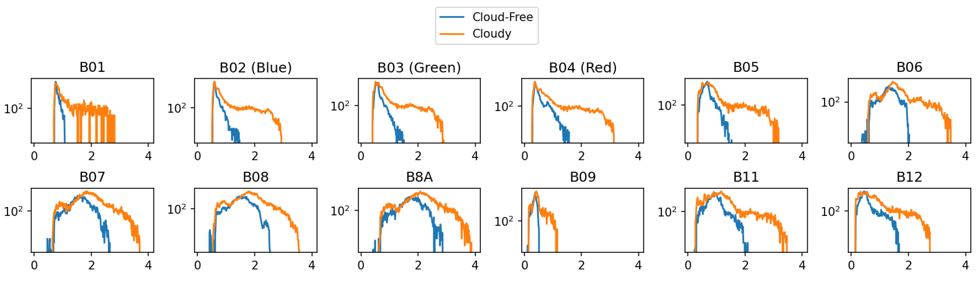
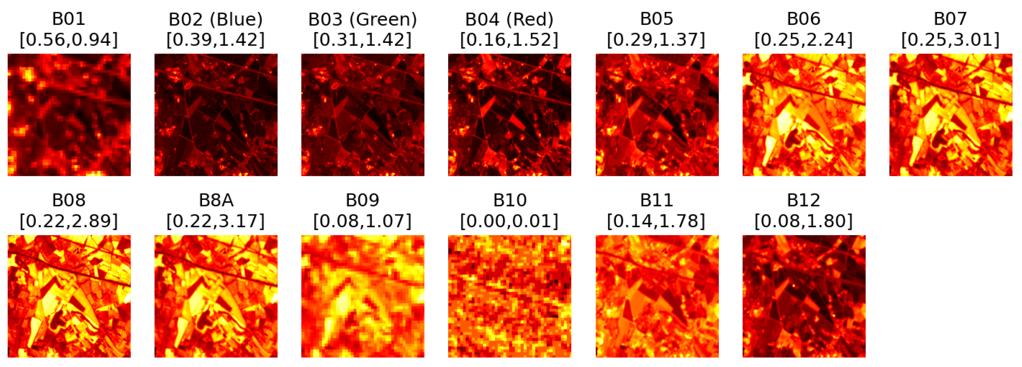
For the task of cloud removal, the dataset of SEN12MS-CR is used, containing real pairs of cloudy and non-cloudy Sentinel-2 images, along with corresponding Sentinel-1 samples. The dataset contains Sentinel-2 Level-1C product, which consists of 13 bands of multi-spectral data. Furthermore, Band 10 is excluded from the experiment, since it primarily responds to the top of atmosphere reflections of cirrus clouds [22], which often have a different effect than in other bands, as can be observed in Figure 19 and Figure 20. This effect is not currently modeled by the cloud simulator and hence the exclusion. The two figures contain visualizations of individual bands from a Sentinel-2 L1C product for a cloudy and a clear sample. In both cases, all bands except for Band-10 (SWIR–Cirrus) appear to be highly correlated. In the cloudy image, the bands tend to contain a similar presence of the cloud, while in Band-10 this object appears absent. Similarly, Band-10 in the clear image appears to detect a fairly different structure than the other bands.

The baseline architecture used for the experiments on cloud removal is DSen2-CR [6], a simple residual-based deep neural network architecture consisting primarily of convolutional operations. In each case, it is trained from scratch to a point where no improvement in validation loss occurs for 30 epochs. The networks are trained using an AdamW optimizer [21] with a starting learning rate of ${10}^{-4}$ and the same decay strategy as the cloud detection model above. Each batch of data contained four clear and four cloudy images, and, similarly to the cloud detection scheme, the loss on the clear images is multiplied by a factor of 0.1. Due to the large dataset size of SEN12MS-CR, during each epoch, the loss is optimized on 1000 random samples from the training dataset, and the validation loss is computed on 500 random samples from the validation dataset.

Similar to the previous example with cloud detection, the models are tested on five different test datasets, one with real clouds and another four with simulated-only data of different cloud types. The commonly used metrics of SSIM (

Table 8. Evaluation on the cloud removal task— (↑) SSIM metric (whole/masked).

Trained on	Real	Thick	Local	Thin	Fog
(a) Real	0.623/0.561	0.619/0.541	0.858/0.668	0.842/0.803	0.740/0.739
(b) Simulated	0.444/0.323	0.474/0.343	0.837/0.530	0.846/0.790	0.669/0.669
(c) Hybrid	0.603/0.538	0.619/0.531	0.873/0.666	0.859/0.814	0.746/0.745
(d) Sim-CSM	0.544/0.462	0.682/0.604	0.899/0.737	0.882/0.846	0.755/0.753
(e) Hyb-CSM	0.567/0.485	0.670/0.595	0.889/0.728	0.872/0.839	0.749/0.748

) and RMSE (

Table 9. Evaluation on the cloud removal task— (↓) RMSE metric (whole/masked).

Trained on	Real	Thick	Local	Thin	Fog
(a) Real	0.217/0.229	0.289/0.323	0.142/0.233	0.165/0.187	0.266/0.266
(b) Simulated	0.884/1.042	1.108/1.271	0.330/0.628	0.300/0.364	0.802/0.802
(c) Hybrid	0.227/0.236	0.303/0.344	0.136/0.247	0.162/0.193	0.276/0.276
(d) Sim-CSM	0.261/0.264	0.198/0.223	0.099/0.170	0.126/0.146	0.196/0.196
(e) Hyb-CSM	0.238/0.251	0.209/0.235	0.107/0.180	0.134/0.154	0.209/0.209

) are used to evaluate the models. Furthermore, each metric is reported for the whole image (the first listed value) as well as the isolated cloud-affected region (the second listed value).

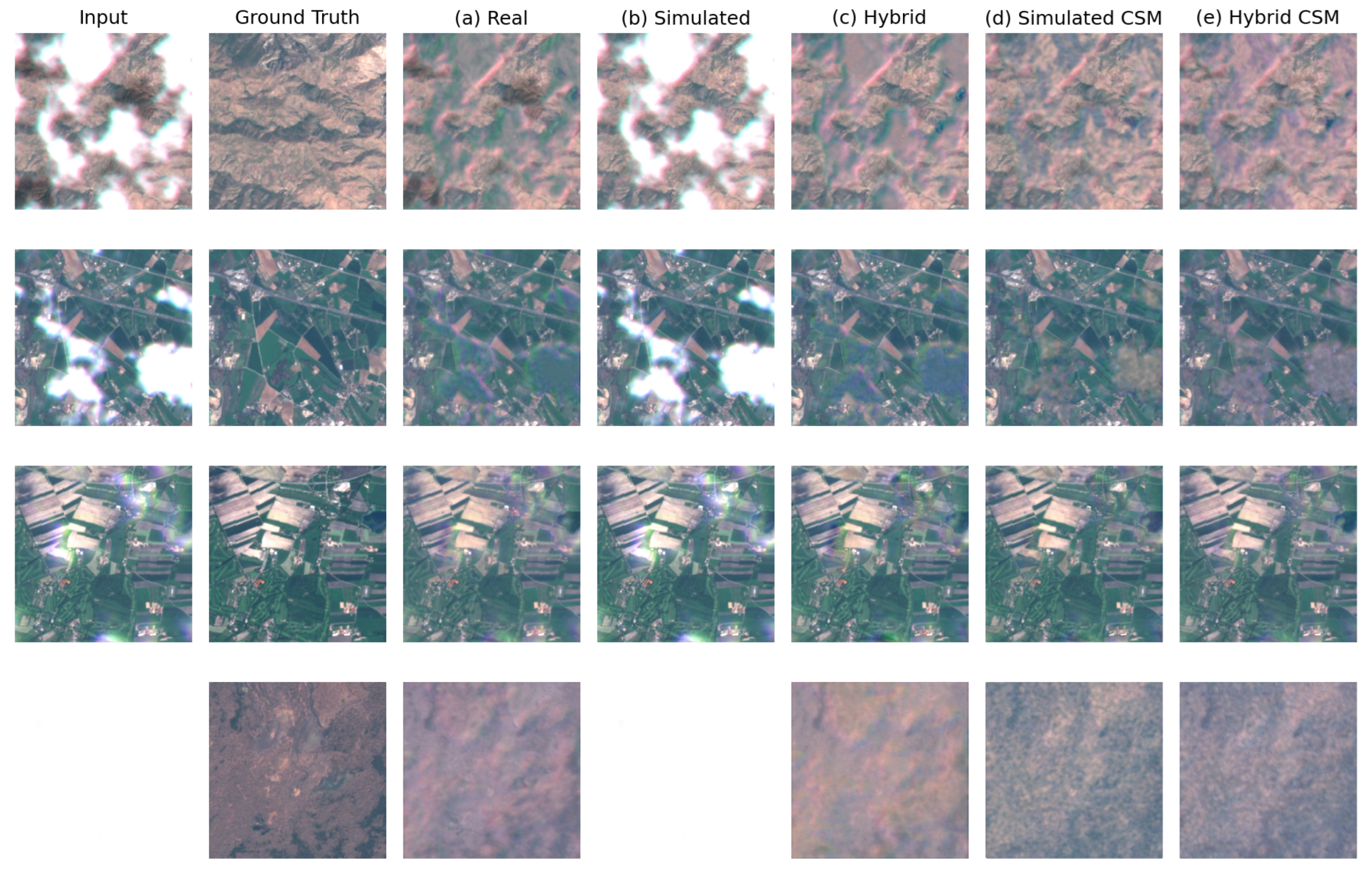
The results in Table 8 indicate that while the model trained on the real data (a) performs best on that type of data (an SSIM of 0.623 for the whole image and 0.561 for the inpainted region), the model (d) trained exclusively on simulated data with channel-specific magnitude achieves an SSIM of 0.544/0.462. On the other hand, for any type of simulated test data, model (d) outperforms model (a). Similar to the detection task, model (b), which was trained on simulated cloudy images without channel-specific magnitude, consistently produces results of the lowest quality. In Figure 21 and Figure 22, it can be observed that model (b) does not really apply any visible changes to the input image, indicating that it does not recognize the cloud objects as something that should be removed. It achieves an SSIM of 0.444/0.323, compared to 0.544/0.462 in the equivalent model trained with channel-specific magnitude. This demonstrates that the channel-specific magnitude feature is crucial for cloud removal models to generalize from simulated data to real instances, indicated by the improved quality achieved with models (d) and (e).

5. Conclusions

This manuscript introduced a novel open-source SatelliteCloudGenerator (https://github.com/strath-ai/SatelliteCloudGenerator, accessed on 22 August 2023) tool for simulating cloudy satellite images with a number of controllable parameters responsible for many features, including cloud structure, locality, color, thickness, or sensing channel misalignment. The tool can be used on image batches directly on GPU and act as an augmentation operation in the PyTorch library commonly used for training deep neural networks.

To shed more light onto the problem, deep neural networks have been trained in the tasks of cloud detection and cloud removal. The results show that learning from simulated data alone has the effect of good performance on real data, especially when channel-specific magnitudes are adjusted. Compared to real data, this approach incurs zero annotation cost. Furthermore, the simulation framework can be used to generate unlimited data for evaluation; in which case, the models trained on simulated data outperform the model trained solely on real data.

Ultimately, neither real nor simulated data appear to be universally more advantageous. The ideal, potentially impossible, case is an abundant source of real images with precise ground truth. Real image sources are not abundant and are likely to contain distorted ground truth. Simulated sources are abundant and with precise ground truth, but a certain gap between real and simulated images can be expected. Given this state of matters, a good way to achieve a trade-off is to perform training as well as evaluation on both data sources, which has been demonstrated herein.

References

1. King, M.D.; Platnick, S.; Menzel, W.P.; Ackerman, S.A.; Hubanks, P.A. Spatial and temporal distribution of clouds observed by MODIS onboard the terra and aqua satellites. IEEE Trans. Geosci. Remote Sens. 2013, 51, 3826–3852. [Google Scholar] [CrossRef]
2. Li, W.; Li, Y.; Chen, D.; Chan, J.C.W. Thin Cloud Removal with Residual Symmetrical Concatenation Network. In Proceedings of the IGARSS 2019—2019 IEEE International Geoscience and Remote Sensing Symposium, Yokohama, Japan, 28 July–2 August 2019; pp. 1974–1977. [Google Scholar]
3. Lin, D.; Xu, G.; Wang, X.; Wang, Y.; Sun, X.; Fu, K. A Remote Sensing Image Dataset for Cloud Removal. arXiv 2019, arXiv:1901.00600. [Google Scholar]
4. Sarukkai, V.; Jain, A.; Uzkent, B.; Ermon, S. Cloud removal in satellite images using spatiotemporal generative networks. In Proceedings of the 2020 IEEE Winter Conference on Applications of Computer Vision, WACV 2020, Snowmass Village, CO, USA, 1–5 March 2020; pp. 1785–1794. [Google Scholar] [CrossRef]
5. Li, J.; Wu, Z.; Hu, Z.; Li, Z.; Wang, Y.; Molinier, M. Deep learning based thin cloud removal fusing vegetation red edge and short wave infrared spectral information for sentinel-2A imagery. Remote Sens. 2021, 13, 157. [Google Scholar] [CrossRef]
6. Ebel, P.; Meraner, A.; Schmitt, M.; Zhu, X.X. Multisensor Data Fusion for Cloud Removal in Global and All-Season Sentinel-2 Imagery. IEEE Trans. Geosci. Remote Sens. 2021, 59, 5866–5878. [Google Scholar] [CrossRef]
7. Ebel, P.; Xu, Y.; Schmitt, M.; Zhu, X.X. SEN12MS-CR-TS: A Remote Sensing Data Set for Multi-modal Multi-temporal Cloud Removal. IEEE Trans. Geosci. Remote Sens. 2022, 60, 1–14. [Google Scholar] [CrossRef]
8. Aybar, C.; Ysuhuaylas, L.; Gonzales, K.; Loja, J.; Herrera, F.; Bautista, L.; Flores, A.; Yali, R.; Diaz, L.; Cuenca, N.; et al. CloudSEN12—A global dataset for semantic understanding of cloud and cloud shadow in satellite imagery. Sci. Data 2022, 9, 782. [Google Scholar] [CrossRef] [PubMed]
9. Xu, Z.; Wu, K.; Huang, L.; Wang, Q.; Ren, P. Cloudy Image Arithmetic: A Cloudy Scene Synthesis Paradigm with an Application to Deep-Learning-Based Thin Cloud Removal. IEEE Trans. Geosci. Remote Sens. 2022, 60, 1–16. [Google Scholar] [CrossRef]
10. Perlin, K. Image Synthesizer. ACM Siggraph Comput. Graph. 1985, 19, 287–296. [Google Scholar] [CrossRef]
11. Dong, W.; Zhang, X.; Zhang, C. Generation of cloud image based on Perlin noise. In Proceedings of the 2010 International Conference on Multimedia Communications, Mediacom 2010, Hong Kong, China, 7–8 August 2010; pp. 61–63. [Google Scholar] [CrossRef]
12. Enomoto, K.; Sakurada, K.; Wang, W.; Fukui, H.; Matsuoka, M.; Nakamura, R.; Kawaguchi, N. Filmy Cloud Removal on Satellite Imagery with Multispectral Conditional Generative Adversarial Nets. In Proceedings of the 2017 IEEE Conference on Computer Vision and Pattern Recognition Workshops (CVPRW), Honolulu, HI, USA, 21–26 July 2017; pp. 1533–1541. [Google Scholar] [CrossRef]
13. Li, J.; Wu, Z.; Hu, Z.; Zhang, J.; Li, M.; Mo, L.; Molinier, M. Thin cloud removal in optical remote sensing images based on generative adversarial networks and physical model of cloud distortion. ISPRS J. Photogramm. Remote Sens. 2020, 166, 373–389. [Google Scholar] [CrossRef]
14. Lee, K.Y.; Sim, J.Y. Cloud Removal of Satellite Images Using Convolutional Neural Network with Reliable Cloudy Image Synthesis Model. In Proceedings of the 2019 IEEE International Conference on Image Processing (ICIP), Taipei, Taiwan, 22–25 September 2019; pp. 3581–3585. [Google Scholar] [CrossRef]
15. Pan, X.; Xie, F.; Jiang, Z.; Shi, Z.; Luo, X. No-Reference Assessment on Haze for Remote-Sensing Images. IEEE Geosci. Remote Sens. Lett. 2016, 13, 1855–1859. [Google Scholar] [CrossRef]
16. Qin, M.; Xie, F.; Li, W.; Shi, Z.; Zhang, H. Dehazing for Multispectral Remote Sensing Images Based on a Convolutional Neural Network with the Residual Architecture. IEEE J. Sel. Top. Appl. Earth Obs. Remote Sens. 2018, 11, 1645–1655. [Google Scholar] [CrossRef]
17. Zi, Y.; Xie, F.; Zhang, N.; Jiang, Z.; Zhu, W.; Zhang, H. Thin Cloud Removal for Multispectral Remote Sensing Images Using Convolutional Neural Networks Combined with an Imaging Model. IEEE J. Sel. Top. Appl. Earth Obs. Remote Sens. 2021, 14, 3811–3823. [Google Scholar] [CrossRef]
18. Makarau, A.; Richter, R.; Müller, R.; Reinartz, P. Haze Detection and Removal in Remotely Sensed Multispectral Imagery. IEEE Trans. Geosci. Remote Sens. 2013, 52, 5895–5905. [Google Scholar] [CrossRef]
19. Sentinel Hub Team. Sentinel Hub’s Cloud Detector for Sentinel-2 Imagery. 2017. Available online: https://github.com/sentinel-hub/sentinel2-cloud-detector (accessed on 22 August 2023).
20. Sandler, M.; Howard, A.; Zhu, M.; Zhmoginov, A.; Chen, L.C. MobileNetV2: Inverted Residuals and Linear Bottlenecks. In Proceedings of the 2018 IEEE/CVF Conference on Computer Vision and Pattern Recognition, Salt Lake City, UT, USA, 18–23 June 2018; pp. 4510–4520. [Google Scholar] [CrossRef]
21. Loshchilov, I.; Hutter, F. Decoupled weight decay regularization. In Proceedings of the 7th International Conference on Learning Representations, ICLR 2019, New Orleans, LA, USA, 6–9 May 2019. [Google Scholar]
22. S2 MPC: Level-1 Algorithm Theoretical Bases Document; Technical Report; European Space Agency: Cologne, Germany, 2023; Ref. S2-PDGS-MPC-ATBD-L1.
Figure 1. The approach of using pairs of real data for training and evaluating cloud removal models often results in fundamental differences in the ground surfaces. Examples from SEN12MS-CR [6]. It is apparent that some areas significantly change their state among acquisitions.
Remotesensing 15 04138 g001
Figure 2. Diagram of the main pipeline of SatelliteCloudGenerator. The tool takes a cloud-free input satellite image I clear and first mixes it with a shadow generated using a shadow generation process (detailed in Figure 4), then blurs the image locally, and finally mixes it with a cloud generated using the cloud generation process (detailed in Figure 3).
Remotesensing 15 04138 g002
Figure 3. Diagram of the cloud generation component responsible for generating the cloud shape using Perlin noise and applying several operations to control the final appearance. The output is a transparency mask and a channel-wise cloud image. The cloud-free source image is used to determine the magnitude of the cloud component in each channel.
Remotesensing 15 04138 g003
Figure 4. Diagram of the shadow generation component. The shadow generation component, similar to the cloud generation component, is based on Perlin noise shape but is followed only by thresholding and range adjustment to produce the output shadow mask.
Remotesensing 15 04138 g004
Figure 5. Demonstration of the Perlin noise generated at several scales (32, 16, 8) (ac) and the result of their weighted sum (d). An example of the resulting cloud mask mixed with a real image is shown in (e).
Remotesensing 15 04138 g005
Figure 6. Example of the clear_threshold of 0.30 applied to the cloud mask from Figure 5. This means that any value less than 0.30 will be clipped to zero, resulting in the black (0.00) regions in the mask (a), which appear as cloud-free portions of the satellite image (b).
Remotesensing 15 04138 g006
Figure 7. Example of mask range adjusted to [min_lvl = 0.0, max_lvl = 0.5] from the original shape. This means that the strongest influence of the cloud in (a) is at 0.5, which corresponds to the reflectance of the ground still contributing to 50% of the value for that pixel, giving the impression of semi-transparent clouds in (b).
Remotesensing 15 04138 g007
Figure 8. Varying levels of locality degree obtained for a range of locality_degree parameter values. For the value of 1, the cloud generates a single Perlin shape with default parameters (a). For the values of 2–4 in (bd), the same Perlin shape is multiplied by another 1, 2, or 3 independent Perlin shapes, resulting in more local (smaller-area) clouds.
Remotesensing 15 04138 g008
Figure 9. Increased locality can also be achieved by adjusting the clear_threshold parameter value (as shown with values between 0.00 and 0.90 illustrated in (ad)), but the cloud edges tend to become sharper, giving the resulting clouds a distinct look, different from the default.
Remotesensing 15 04138 g009
Figure 10. An example of a sample with channel-wise misalignment controlled by the channel_offset parameter. Without this effect, the cloud component is fully aligned across image channel as shown in (a). However, to simulate a common feature of satellite images, a small spatial shift can be introduced to individual channels as shown in (b), resulting in what often appears as colored cloud edges as in (c).
Remotesensing 15 04138 g010
Figure 11. An example of a cloud with color adjusted by the ground reflectance. To simulate the global light reflected from the ground affecting the cloud color, the cloud image (a) is adjusted, depending on the thickness of the cloud, to a value between the mean reflected color of the ground and pure white, before it is used for the mixture (b).
Remotesensing 15 04138 g011
Figure 12. Example of cloud-free (b) and cloudy (c) regions masked from a real cloudy sample (a) using the s2cloudless cloud detection tool. This allows us to approximate the reflectance characteristics of the cloud-free and cloudy regions separately.
Remotesensing 15 04138 g012
Figure 13. Histogram curves for the example image. In each case, it is shown that the cloudy region (orange plot) contains higher values but also exhibits some resemblance to the cloud-free histogram (blue) due to the leakage of the ground component in the cloudy region (as shown in Figure 12).
Remotesensing 15 04138 g013
Figure 14. Example of a sample simulated with (c) and without (b) channel-specific magnitude (CSM) scaling. The real image reference used for magnitude scaling is shown in (a).
Remotesensing 15 04138 g014
Figure 15. An example of a shadow generation feature. In this case, the mask (a) determines which regions of the ground image will appear darker, resulting in an image with shadows (b).
Remotesensing 15 04138 g015
Figure 16. An example of the cloud-dependent ground blur effect. Before mixing with the cloud, the cloud-free image is blurred with the strength of the effect proportional to the thickness in the cloud mask, as shown in (a). This is later followed by the standard mixture process to give the final result (b) with a cloud on top of a locally blurred ground image.
Remotesensing 15 04138 g016
Figure 17. Random samples synthesized using 4 different CloudGenerator configurations used for this work. The configurations contain parameters that can easily adjust the visual appearance of clouds, as listed in Table 1.
Remotesensing 15 04138 g017
Figure 18. An example of a precise segmentation mask derived from the simulation tool. It is possible to obtain an accurate segmentation representation for the simulated data, since the cloud mask is generated explicitly as part of the simulation process.
Remotesensing 15 04138 g018
Figure 19. Example of content of individual multi-spectral bands in each channel for a cloudy Sentinel-2 L1C image. Intensity range for each band is listed in square brackets.
Remotesensing 15 04138 g019
Figure 20. Example of content of individual multi-spectral bands in each channel for a cloud-free Sentinel-2 L1C image.
Remotesensing 15 04138 g020
Figure 21. Examples of cloud removal output for the five model variants on real cloudy images.
Remotesensing 15 04138 g021
Figure 22. Examples of cloud removal output for the five model variants on simulated cloudy images (test images simulated with channel-specific magnitude).
Remotesensing 15 04138 g022