Abstract
This work proposes an active learning (AL) methodology to create models for the segmentation of fire and smoke in video images. With this model, a model learns in an incremental manner over several AL rounds. Initially, the model is trained in a given subset of samples, and in each AL round, the model selects the most informative samples to be added to the training set in the next training session. Our approach is based on a decomposition of the task in an AL classification phase, followed by an attention-based segmentation phase with class activation mapping on the learned classifiers. The use of AL in classification and segmentation tasks resulted in a 2% improvement in accuracy and mean intersection over union. More importantly, we showed that the approach using AL achieved results similar to non-AL with fewer labeled data samples.
1. Introduction
Forest fires are one of the most challenging and devastating issues societies have been facing for the past decades. Current consequences of climate change have significantly increased the risk of wildfires. In Portugal alone, in 2017, close to 540,000 hectares were burnt [1]. Additionally, in [2], it was estimated that between 2002 and 2016, EUR 150 million was lost every year due to fires.
Methods relying on human observation, from either lookout towers, aircraft, or reports by citizens, have been proved to be affected by error. On the other hand, the usage of automatic systems to augment human operators during observation has become extremely attractive since their performance has improved and it provides uninterrupted analysis of video feeds [3]. In particular, automatic methods that perform image segmentation, with the labeling of individual pixels, offer a high level of detail, when compared with a simple image classification or image detection (typically with a bounding box encompassing the area of interest) [4]. This detail in the image space is useful in the analysis of wildfires because, when the pixels are georeferenced, it results in a detailed map of the areas affected by the fire or smoke [5].
Despite the introduction of some datasets, research in the area of fire and smoke detection has some limitations, particularly on the low availability of datasets and labeled data [6,7]. Adding to the previous issue, data are often available in the form of weak labels (indicate the presence, or not, of fire and/or smoke). Finally, remote sensing images often have a perspective and scale quite different from generic image segmentation and require models to be adapted [8]. Considering the mentioned issues, our task can be summarized as training a deep learning segmentation model, with fewer weakly labeled samples but still achieving a performance relevant to smoke and fire detection.
An active learning (AL) approach was considered since this learning method can reduce the number of samples necessary to obtain a good model [9]. The goal of this work is to develop deep learning methods for fire and smoke segmentation on low amounts of labeled data. With this goal in mind, the main contributions of this paper are as follows:
- Proposal of a method that reduces the amount of labeling effort by using weakly supervised learning coupled with active learning;
- Demonstration of the superior performance of the method in the fire/smoke analysis when compared with non–active learning approaches;
- Assessment of the parameters’ influence on the active learning process.
The remainder of the paper is organized as follows: Section 2 presents some of the challenges for fire and smoke analysis and also presents some alternatives for this task. Section 3 details the method that was selected in this work. Section 4 describes the data and the model’s parameters that were used in the experiments used to assess the proposed method. Section 5 presents and discusses the results obtained in the experiments. Finally, Section 6 presents the main conclusions and future work.
2. Background and Related Work
2.1. Active Learning
In deep learning, there is a strong correlation between the quality and quantity of the data used to train networks and their performance on the target task [10]. However, collecting large-scale datasets with accurate annotation is very expensive [11]. AL methods [9] are a way to solve this problem, by reducing the amount of data necessary to achieve the desired results. AL is a field of machine learning where the key idea is that the algorithm can query an oracle (user, machine, dataset, or some other information source) to label a relevant unlabeled data instance. An AL framework allows the algorithm to be “curious” and to choose the data it wants to learn from, therefore achieving the desired results, desirably, with less data.
The algorithm uses an acquisition function to create the queries. An acquisition function is the block that determines which data instances should be queried, to be labeled in order to accelerate the network’s learning process. The fundamental concept behind an AL framework is that, with fewer labeled examples, a learning algorithm can have a better-performing model (with better accuracy), if the model can efficiently select the most informative samples to learn from, and improve the learning process. This idea is really strong for critical applications, where it might be difficult, expensive, or even unethical to obtain training samples to enrich a dataset. Some examples of such applications are healthcare [12,13], autonomous driving [14], or fire detection considered in the present work.
There are three categories of AL: stream-based selective sampling, pool-based sampling, and membership query synthesis. The idea behind the first one is that the algorithm determines if it wants to query for a label or not, while the data are being presented to the algorithm. In the second one, the algorithm evaluates the entire dataset before making a selection of the queries. In the third one (only applicable in some cases), the algorithm creates its own examples to query. In a fire/smoke analysis task, the biggest workload is the annotation of images, while gathering the images is relatively fast. Based on this fact, we considered AL methods using pool-based sampling.
2.2. Fire and Smoke Detection and Segmentation
The need to formulate an efficient method of detecting fire and smoke has produced many different approaches in the area of deep learning. These approaches encompass different tasks, such as detection and segmentation, but also different learning methodologies, such as fully supervised, weakly supervised, and self-supervised. In [6,15,16], three fully supervised approaches to tackle this problem are described. Ref. [15] employs a specific CNN-based smoke detection and segmentation for both clear and hazy environments. Ref. [16] develops a method based on the motion characteristics of smoke. Ref. [6] uses faster R-CNN with synthetic forest fire smoke images in order to combat the problem of false positives (due to the existence of fire, but not smoke).
A condition that limits the performance of these algorithms is the existence of very few datasets that are fully labeled or labeled at all. To solve the problem of the low availability of datasets with pixel-level annotations, the developers of [17] use a weakly supervised approach, making use of only image-level labels and datasets to create the segmentation masks of the images of fire and smoke. In [18], the developers explore the area of self-supervised learning. In the first phase, a model was trained to perform certain tasks (pretext tasks) on unlabeled data in the task of recognition of the features present in forest fires. In the second phase, using the previous model, in addition to very small sets of labeled data, it was possible to train the final classifier. In [19], the authors use a semisupervised methodology to perform semantic segmentation of fire and smoke imagery using a generative adversarial network (GAN). Even though it was deduced that a semisupervised GAN seemed beneficial for the task of fire and smoke segmentation, these results are not statistically significant and still need to be validated by running more experiments. Another application of GAN, in [20], is used to solve the overfitting problem.
3. Methodology
3.1. Active Learning Considerations
In [21], an analysis of recent AL-based image classification methods is presented and benchmarked on the MNIST [22], CIFAR-10 [23], and a medical pneumonia [24] dataset. It is shown that deep evidential active learning (DEAL) [21] consistently outperformed all the other frameworks in all the datasets.
The DEAL algorithm selects the most informative samples to query. It performs this through the use of an acquisition function that applies the minimal margin uncertainty measure to all the unlabeled samples and chooses the sample with the smallest margin (the most uncertain). The minimal margin is determined by calculating the difference between the two most probable classes for a sample. If the difference of probability between these two classes, for a given sample, is small, it means that the algorithm is not sure to which class that particular sample belongs, and thus, it is highly informative and can be sampled by the acquisition function.
One of the most common activation functions used in the output layer of CNNs is the Softmax activation function. However, a model can still be uncertain despite the output of the Softmax function being high. To solve this, the author proposes the use of the Softsign activation function and uses the outputted values as an evidence vector for the Dirichlet distribution to better model the probability of each class. By implementing this, a degree of quantification of the uncertainty is introduced, and the class probabilities’ results are improved.
3.2. Segmentation Methodology
To perform image segmentation, we base our research on methods used in [17], which performs weakly supervised segmentation (WSS) by inputting an image to the classification model (trained without an AL framework), performing the prediction, and retrieving the features of the image that contributed most to the classification. To perform this, the following methods were used.
3.2.1. Class Activation Mapping
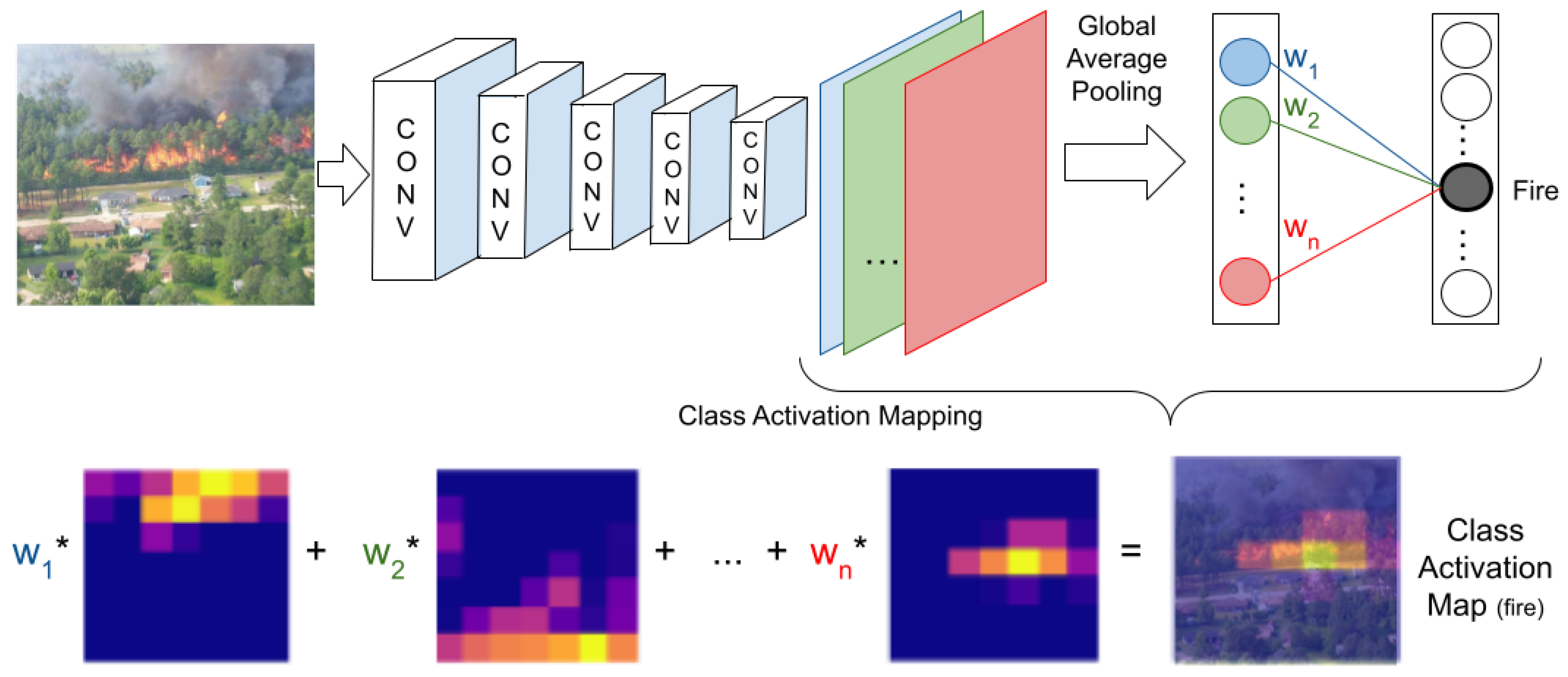
The core concept of CAM, described in [25], is that a model develops localization capabilities even when being trained solely on image-level labels. To perform this, only the backbone of the classifier CNN is used, removing the fully connected layers and adding a global average pooling (GAP) layer after the convolutional layers. The reason for this is that the fully connected layers remove the spatial information provided by the convolutional layers. The goal of the GAP layer is to output the spatial average of each feature map’s last convolutional layer. To obtain the class activation maps themselves, a weighted sum of each of the feature maps is performed, which then generates the final output. Thus, the class activation maps can be defined by
where is the class activation map for class c. is the activation of the feature channel n at the location in the last convolutional layer. is the weight for class c and unit n. A visual representation of the CAM method can be visualized in Figure 1.
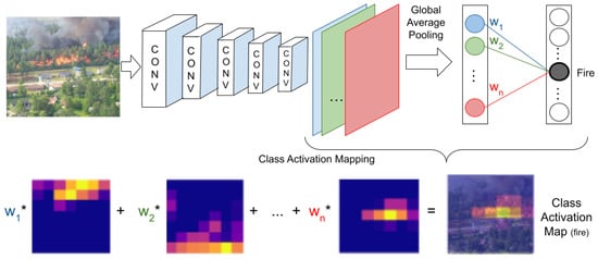
Figure 1.
CAM method developed by [25]. Image adapted from [25].
Finally, a fully connected layer is added with the sigmoid activation function (instead of Softmax, since the sigmoid is used for binary classification). The size of the fully connected layer is two due to the fact that we have a network for each of the methods (fire and smoke) and the two classes represent the presence or lack of presence of each of the elements. For the fire version and for the smoke version, VGG19 and VGG16 were used correspondingly. The mapping resolution for both methods is 16 × 16.
3.2.2. Conditional Random Fields
For the CRF implementation, we follow the methodology of [26,27]. The goal of the CRF is to take the results (mask) provided by the CAM and the contextual neighboring information existing in the image, and form a more accurate segmentation of the class we are analyzing.
In this postprocessing phase, the image is represented as a graph, where every pixel is connected and is treated as a CRF node. Each of these nodes has a unary potential, written as
where is the label assignment for pixel m; thus, denotes the probability of pixel m to be assigned to class n. For every pair of nodes, there is a link that expresses their compatibility and is represented by a pairwise cost. The pairwise cost is defined as
with for and zero otherwise. As presented, the pairwise cost also contains two Gaussian functions: one that only depends on spatial distance between pixels m and n and another that depends on the distance and also on the difference in color, , between those two same pixels. The remainder parameters , , , , and control the relative contribution of each Gaussian function.
The CRF algorithm iteratively minimizes the energy, which corresponds to the sum of all unary and pairwise costs:
3.3. Cost-Effective Active Learning Methodology
Since the DEAL method also modifies the activation function to improve the classification results, the implementation of the class activation mapping (CAM) method (that implies the modification of this structure, previously explained in Section 3.2.1) might be compromised. Therefore, to counter this, we decide to apply the approach developed in [28] (cost-effective active learning (CEAL)), in which the authors apply only the first segment of the DEAL algorithm (minimal margin sampling). Adding to that, when benchmarking the different AL algorithms in [21], the CEAL method proved to be the second-best-performing algorithm, and was only outperformed by DEAL.
As mentioned previously (Section 3.1), despite CEAL [28] not being the best-performing AL framework (outperformed by DEAL [21]), it was the best to evaluate the performance of an AL structure and to compare it with non-AL frameworks. With this idea in mind, the main factor that determines the efficiency of the AL algorithm is the method from which it acquires the new samples, known as acquisition function. In CEAL, the acquisition function is the minimal margin sampling, defined as
where represents the sample; constitutes its label; and represent the first and second most probable classes; represents the unlabeled dataset, from which the sample is retrieved; and denotes the probability of sample belonging to class . The lower the value of , the more uncertain the classifier is about the class of the evaluated sample, and therefore, in theory, the most informative the sample is. After applying (5) to all unlabeled samples, these are ranked in ascending order by the values determined by . Considering an acquisition size of k, the k first-ranked samples are added to the training set.
To initialize the process, the model is pretrained on a subset of samples defined by the user and uniformly sampled, known as warmstart size W. After the first model is trained, the acquisition function is used to obtain k samples of the unlabeled set, with k being defined by the user, known as acquisition size. Then, the model is iteratively retrained, until one of two options is met: there are no more samples to be added to the training set, or the computational resource budget (memory, training time) has been reached. This approach is formalized in Algorithm 1.
The model V that is mentioned in Algorithm 1 is a classifier, and in the proposed method, the selected classification networks were VGG16 and VGG19 for smoke and fire, respectively. The choice of these networks over many other options was solely to enable a direct comparison with the method proposed by [17]. It is worth noting that we purposely kept all the cited model’s configurations to have an adequate comparison. Since the cited work uses WSL but does not uses AL, the comparison highlights the contribution obtained with AL.
| Algorithm 1 CEAL algorithm with minimal margin acquisition function |
Input: Unlabeled set , labeled set , acquisition size k, warmstart size W Output: Updated model V Procedure: Uniformly sampled W datapoints from unlabeled set Label by expert W samples and add to labeled set Remove W selected samples from unlabeled set Train initial model V with labeled set while and budget available do Load model V Compute (5) for all samples of the unlabeled set Sample k most informative samples from unlabeled set Label k most informative samples and add to labeled set Remove k selected samples from unlabeled set Train model V with labeled set Save model V end while |
3.4. Model Developed
The input for the proposed system is red green blue (RGB) imagery, retrieved from surveillance platforms (aircraft or towers). The output consists of segmentation masks that indicate the presence of fire and/or smoke. The main aim of our model is to improve the work performed in [17] by enhancing the classification model with an AL methodology. Since AL presents queries (for the oracle, in the case of our experiments, the oracle was actually a part of the dataset’s labels that were kept “hidden” from the learning algorithm; thus, a given label was only provided when the AL algorithm queried that label, simulating the labeling that an expert would provide in a real case to label the most informative examples) and improves the learning process, the model could achieve the desired results with potentially less data. The classification model implemented is the CEAL method. The labeled dataset uses weak labels (positive/negative for the presence of fire/smoke), which maintains the main advantage of the original work, allowing for a fairly simple process of labeling samples.
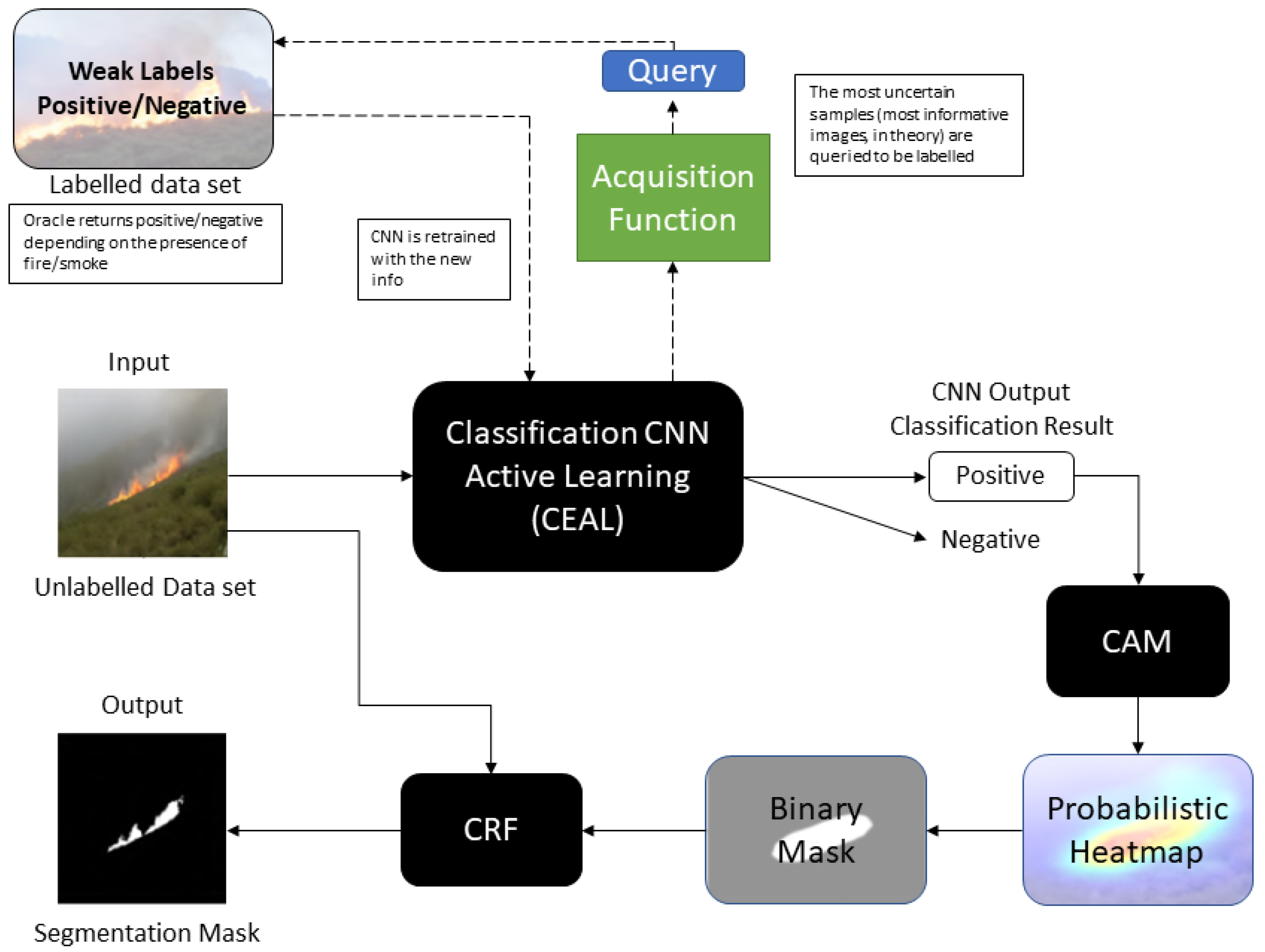
After performing the classification task, the image is fed to the segmentation phase, more specifically to CAM, where the more relevant parts of the image are highlighted. These relevant parts, which contributed the most to the prediction of the classification model, are highlighted in Figure 2 with a probabilistic heatmap, which is then converted to a binary mask. To improve on the results obtained in the binary mask, a postprocessing stage is introduced by the use of CRF. The CRF method analyzes the neighboring context, which, in this case, corresponds to the color and spatial information associated with the original CAM binary mask, to output a better-defined segmentation mask. A diagram of this method can be observed in Figure 2.
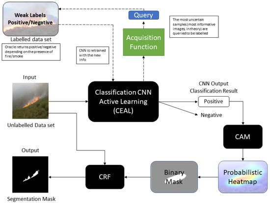
Figure 2.
Structure of the proposed approach.
4. Experimental Setup
4.1. Datasets
Two types of datasets had to be used, one with image-level labels and one with pixel-level labels. The dataset with image-level labels was used to train the entirety of the models and to validate and test the different classification models. The one with pixel-level labels was used for the evaluation of the segmentation phase.
4.1.1. Image-Level Labels
This dataset is composed of images that have an individual label assigned to each image. The presence of a given class is always either positive or negative. For the fire examples, the source of the samples was the dataset available in [7], with negative examples retrieved from the internet. For the smoke examples, the positive samples were retrieved from [29,30], and once again, the negative samples were gathered from the internet. The total number of gathered samples was 1806. Since fire and smoke are, for the most part, intrinsically related and often present in conjunction, all the gathered samples can be applied to train both models. The dataset is unbalanced, as it contains 70% of positive samples and 30% of negative examples, for both the fire and smoke classes. The dataset is split in 78% of samples (1408) for the training set, 12% of samples (217) for the validation set, and 10% of samples (181) for the test set.
4.1.2. Pixel-Level Labels
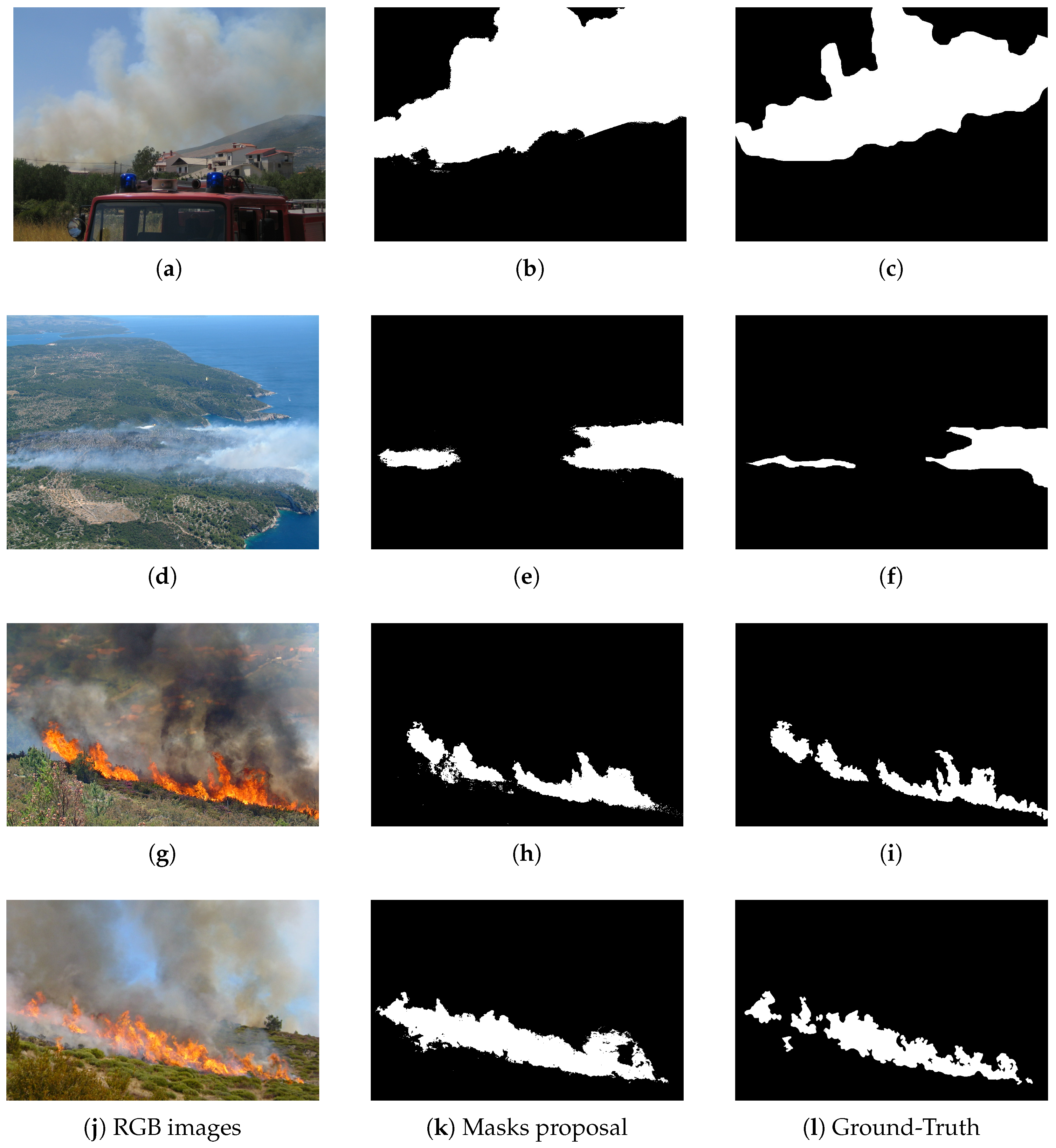
Due to the specific nature of pixel-level samples, the number of available images is significantly smaller; therefore, the gathered number of ground truths (GT) is consequently small. The source used to collect the fire and smoke GT was once again [7,29]. The data composition of the gathered samples is made by 595 samples of fire and 112 samples of smoke. An example of the pixel-level samples can be observed in Figure 3.
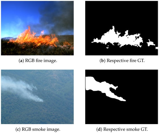
Figure 3.
Pixel-level samples for the fire and smoke dataset.
4.2. Model Setup
4.2.1. Classification Model
We use as a baseline the models developed in [17] and described in Table 1.

Table 1.
CNN classification model parameters.
Some differences in the parameters between our approach and the one developed in [17] are made to improve the training of the AL methodology. In our models, we did not use ImageNet pretrained weights [31]. The difference between using pretrained weights and training from scratch proved to be almost insignificant. Therefore, to better evaluate the impact of AL and its ability to improve the model results, the use of ImageNet weights was not implemented and, instead, Glorot’s method was used to initialize the weights [32].
In our experiments, we analyze different AL parameter settings. The two main parameters related to AL training are acquisition size and warmstart size. Acquisition size is the number of unlabeled samples that are selected by the acquisition function to be added to the training set in each AL round. Warmstart size is the number of uniformly selected samples on which the initial model is trained.
4.2.2. Segmentation Model
For the segmentation model, we use the optimal parameters, found by the original work of [17], in Table 2. We note that the parameters of the segmentation model are not learned from data, so we use the values existing in our baseline model.

Table 2.
CRF and CAM parameters.
5. Experimental Results
A qualitative inspection of the results obtained with the proposed approach indicates segmentations that approximate the areas with fire and smoke, as shown by the examples in Figure 4. To demonstrate the merit of the AL approach, we designed several experiments with the following objectives: assess the influence of the warmstart size, compare AL models with non-AL models, and assess the influence of the acquisition size. The design of the experiments was also impacted by the overall architecture, since the complete model is based on a classifier, which is then used to perform segmentation. The AL approach only operates on the classification task; it is important to assess if AL has an impact on this task and if any benefit propagates to the segmentation task. The three previously described objectives were then tested for the two task, as presented in Table 3.

Figure 4.
Example of image segmentations for both fire and smoke.

Table 3.
Combination of conditions verified in the experiments and the respective reference code that was assigned.
Since two different tasks were considered in our experiments, we also used different evaluation metrics. For the case of classification, we used accuracy, which measures how well the model can make correct predictions. It outputs the ratio between the number of correctly predicted image samples and the total number of image samples, thus computed as
For the segmentation task, we used Intersection over Union (IoU). IoU indicates how well the area predicted to belong to a class overlaps with the actual area of the class provided by the annotation. It is computed as
5.1. Experiment A.1
The purpose of this experiment was to assess how the initial number of samples, on which a model is trained (warmstart size), can influence the following AL rounds and the model learning curve. Adding to that, we aim to find the optimal number of samples to which applying additional AL rounds may not benefit the model any further.
The problem of assessing the influence of the initial number of training samples comes from the objective of reducing the number of AL rounds and potentially reducing (or optimizing) the total training time. Since each AL round consists of training an entire model (on a given labeled set that is incrementally getting bigger), with the model weights of the previous AL round, the total training time can significantly add up, if the initial training size is set too low. Therefore, the training time is strictly related with the number of AL rounds run. For example, by doubling the number of AL rounds run (number of models trained), the training time would also be expected to double.
To perform this analysis, a set of parameters was defined. For the acquisition size, the size was set to 32 samples. For the warmstart size, multiple values were selected, and models were run for warmstart sizes of 1% (14 samples), 10% (141 samples), 20% (282 samples), 35% (493 samples), 50% (704 samples), 65% (915 samples), and 80% (1126 samples) of the total training set. From the obtained results, three deductions could be retrieved. First, in terms of learning, it was possible to observe from the test set, in Figure 5, that there is not any benefit in running additional AL rounds past the 400-sample mark in the case of fire, which corresponds to 28% of the complete dataset, and 800-sample mark in the case of smoke, which corresponds to 57% of the complete dataset. At this point, the test set accuracy barely increases past 96.5% for fire and 88% for smoke, increasing ever so slightly until it reaches an accuracy of 97.45% and 89%, respectively. Second, for dataset sizes lower than the values of stagnation (state where the model’s accuracy has stopped or is growing very slowly), it is massively beneficial to choose lower warmstart sizes.
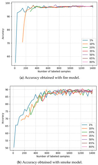
Figure 5.
Evolution of classification metric accuracy for both fire and smoke AL models with different warmstart sizes and a fixed acquisition size (32) in the test set (experiment A.1).
5.2. Experiment A.2
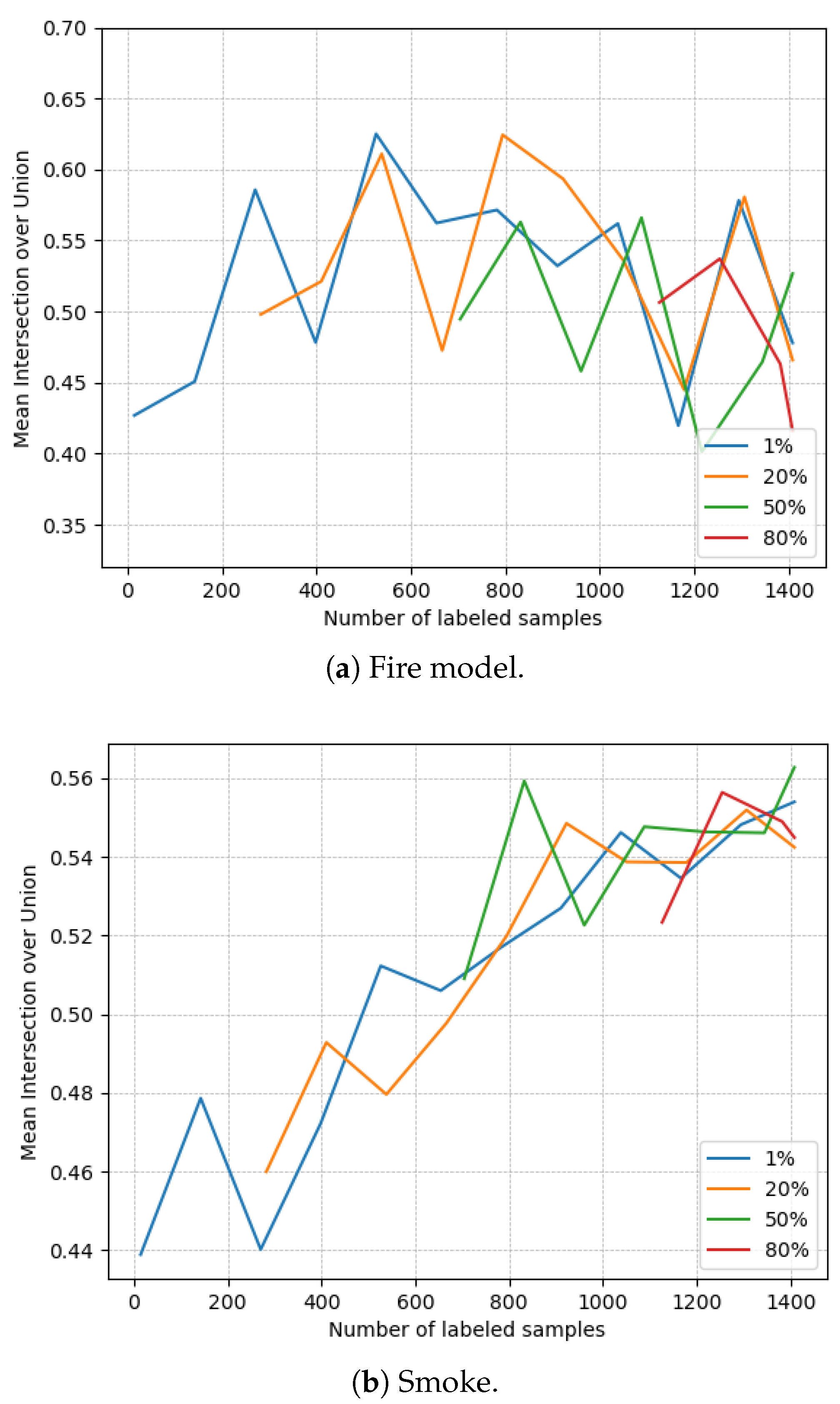
The purpose of this experiment is to evaluate the influence of the warmstart sizes and address if the segmentation results suffer from any kind of beneficial or detrimental influence when running multiple AL rounds on the final trained model. The models analyzed have warmstart sizes of 1% (14 samples), 20% (282 samples), 50% (704 samples), and 80% (1126 samples) of the training set. For this experiment, we select an acquisition size of 128.
The gathered results of fire and smoke can be observed in Figure 6. It was possible to observe that the model mean intersection over union (mIoU) rose until, approximately, the 500-sample mark (36% of the total dataset); meanwhile, in experiment A.1, Section 5.1, the model’s accuracy only rose until the 400-sample mark (28% of the total dataset). A possible explanation for this difference could be derived from the difference in the acquisition size used. In this experiment, the acquisition size set was 128, while in the the previous experiment, it was 32. This divergence could justify the dissimilarity in the number of samples needed for the model to achieve its optimal state. Adding to this, an acquisition size this big does not allow us to observe if the model could have achieved better results with fewer samples because the jumps in acquisition size are too big. It was also possible to notice that after the 500-sample mark, the mIoU became unstable and, over time, gradually reduced the overall results. Therefore, it is possible to theorize that, after a given number of samples, the samples that are selected in the next AL rounds are less informative and produce some form of overfitting that also affects the segmentation. Given these results, it could be possible to hypothesize that in AL models, to achieve the model’s optimal state (best results for the lowest number of samples possible), the most important parameter could the number of AL rounds run. The influence of the warmstart size is solely a way to speed up the training time, but in return, the model will need even more samples to achieve this optimal state.
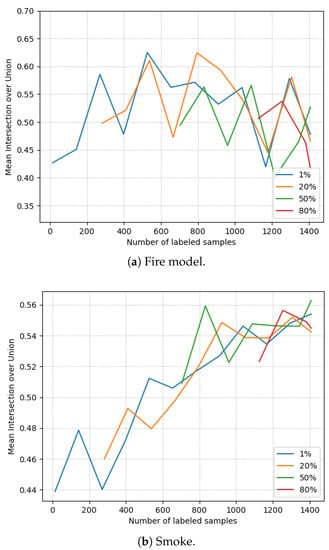
Figure 6.
Evolution of segmentation metric mean intersection over union (mIoU) for AL models with different warmstart sizes and a fixed acquisition size (128) in the test set (experiment A.2).
From the smoke results, we can see that until the 1000-sample mark, the mIoU values increased, and after that, the model stabilized. Comparing with the classification results from the previous experiment, a 200-sample difference occurs in the obtained results in experiment A.1 (Section 5.1) and in this experiment. The justification for this could be the same as the one provided for the fire results: because the acquisition size is significantly bigger, the number of samples to achieve the optimal state also increases. Just as in the fire dataset, it is possible to assess that the main advantage of changing the warmstart size comes from the time-saving bonus. However, if the goal is to achieve the optimal model in the least amount of samples, a small warmstart size and acquisition size should be set in order to allow for the algorithm to select the most informative samples earlier.
To better test this hypothesis, further ahead, in experiments C.1 and C.2 (Section 5.5 and Section 5.6), tests on the acquisition sizes were run.
5.3. Experiment B.1
In this experiment, the goal was to assess the differences between AL models and non-AL models. Particularly, the main objective is to evaluate if a model, when faced with the opportunity of choosing the most informative data to learn from, will obtain better results than a model that cannot choose the data it learns from. To perform this, the initially selected samples of the AL models are introduced in the set used to train the non-AL model. This way, we guarantee that, independently of the AL model final results, these are consequences of the sampling performed by the acquisition function. The acquisition size is maintained at 32.
For the fire dataset, we compare the results of AL and non-AL models trained up to 282 samples. This number is selected from the fact that, in the previous experiment, models with more than 400 samples did not improve the results any further; therefore, we chose a lower number to verify the effects of AL. Adding to this, we train three different models with distinct warmstart sizes: 90, 154, and 218 samples. The purpose of these different warmstart sizes is to observe how the different numbers of AL rounds can change the results. From the obtained results, presented in Table 4, it is possible to observe that the accuracy of the AL models was better when compared with the non-AL model.

Table 4.
Comparison of accuracy between models trained with and without AL (experiment B.1) in the fire dataset.
For the case of smoke, we compare the results of AL and non-AL models trained up to 422 samples. Just like in the case of fire, we selected this number to be lower than 800 samples, since this was the number from which the models did not improve any further. We also train three different AL models with distinct warmstart sizes: 102, 198, and 326 samples. Once again, the purpose of these different warmstart sizes is to observe how the different numbers of AL rounds can change the results. The obtained results of the smoke comparison are in Table 5, where we see that the accuracy of the AL models was better overall when compared with the non-AL model. Therefore, for both fire and smoke, we can say that, on given small datasets, both classes can benefit from AL to improve its results.

Table 5.
Comparison of accuracy between models trained with and without AL (experiment B.1) in the smoke dataset.
5.4. Experiment B.2
In this experiment, we have the same goal as in experiment B.1, but now applied to the segmentation. Once again, the goal is to evaluate if we achieve better results with the AL approach as a consequence of the sample selection process, when comparing with the random selection followed by the non-AL methods. Here, we apply the exact same setup as in experiment B.1, with the exception that, instead of analyzing the accuracy and loss of the models, we analyze the mIoU.
For the evaluation of the fire segmentation results, Table 6 collects the data obtained. By assessing these results, we can observe that the mIoU of AL models was better than the non-AL model.

Table 6.
Comparison of the segmentation metric between models trained with and without AL (experiment B.2) in the fire dataset.
For the smoke segmentation results, a comparison between the segmentation results is in Table 7. Just like in the fire results, we observe that both mIoU values of AL models were better than the non-AL model. Considering the presented results, overall, there is some evidence that on a given small dataset, fire and smoke models could benefit from AL to also improve the segmentation results.

Table 7.
Comparison of the segmentation metric between models trained with and without AL (experiment B.2) in the smoke dataset.
5.5. Experiment C.1
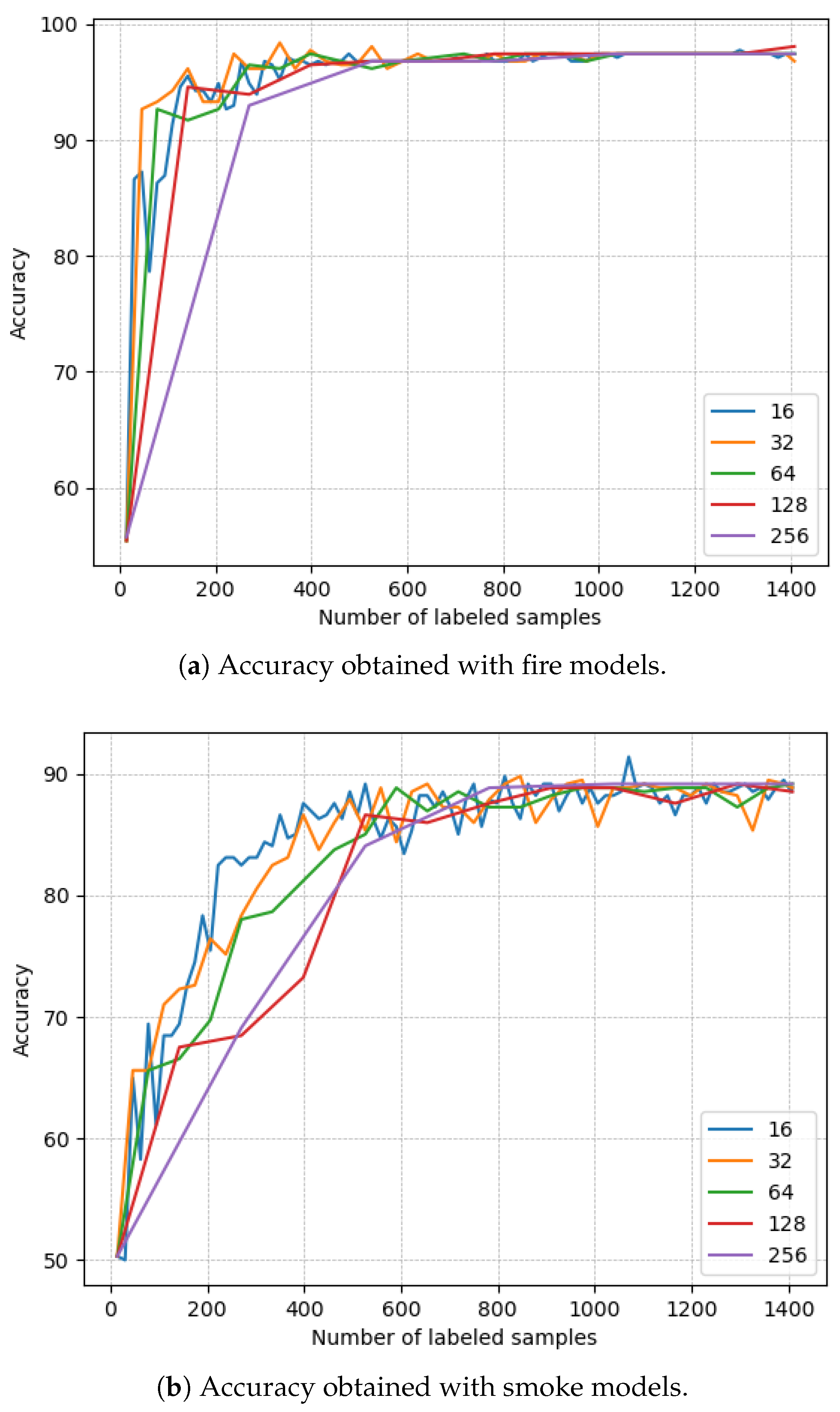
In this experiment, the aim is to evaluate the influence of the acquisition size in the learning process. By changing this parameter, we are changing the number of samples that are added to the training set in each round and, as a consequence, the number of AL rounds that are run to train the model. This means that the lower the acquisition size, the higher the number of AL rounds. The results for the acquisition sizes 16, 32, 64, 128, and 256 are compared. To guarantee the maximum number of AL rounds, the warmstart size is set to 1% of the total samples (14 samples). The gathered results for fire and for smoke are both in Figure 7. For the fire model, it is evident from the data that setting the acquisition size to a value too high was not optimal. This is particularly noticeable for an acquisition size of 256. Setting an acquisition size too high will not be ideal for the learning process, increasing the total number of samples needed to achieve optimal results. On the contrary, setting the acquisition size too low also produced some overfitting (particularly noticed for an acquisition size of 16). The number of AL rounds needed to achieve optimal results in the fire dataset was not high.
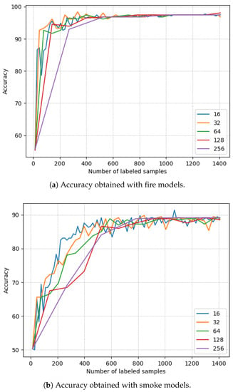
Figure 7.
Evolution of classification metric accuracy for fire and smoke AL models with different acquisition sizes and a fixed warmstart size (1% of the total dataset) in the test set (experiment C.1).
In the case of smoke, as it can be seen, the use of lower values for the acquisition size significantly decreases the number of samples needed to achieve the desired results. An acquisition size of 16 can, in some instances, obtain the same accuracy for almost half the needed samples, when compared with the accuracy values of the 128 and 256 acquisition sizes. Therefore, in the case of smoke, the acquisition size plays a massive role in the number of samples needed to achieve optimal results, allowing the model to reach the optimal state with much fewer samples.
Overall, setting lower acquisition sizes (increasing the number of AL rounds) proved to be beneficial to the learning process; however, setting this value too low could, in some cases, produce overfitting.
5.6. Experiment C.2
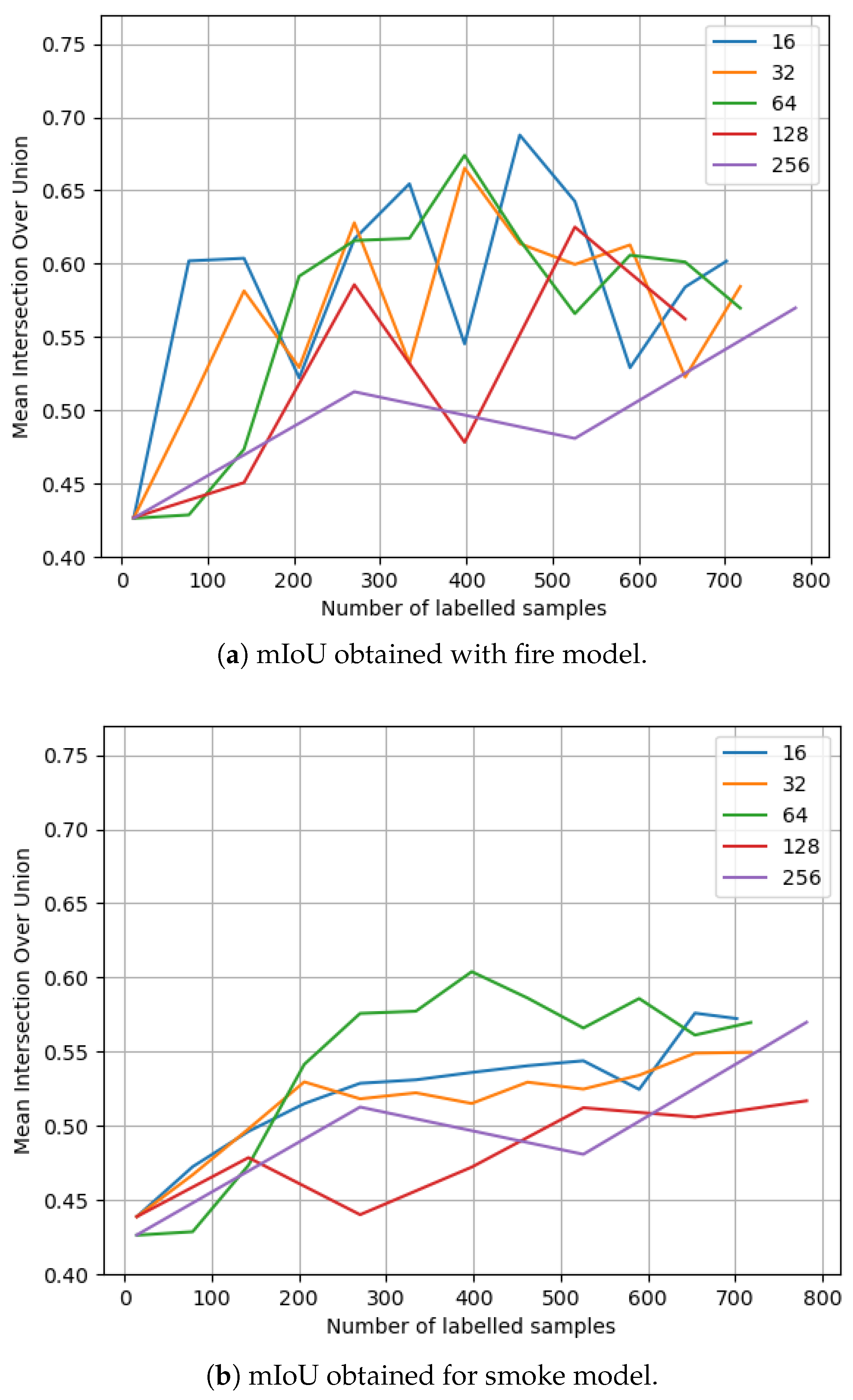
It has been already deduced, from the previous experiment C.1, in Section 5.5, that by changing the acquisition size, it could be possible to impact the number of samples needed to achieve better results. In this experiment, we evaluate if the same principle applies to the segmentation process. To do so, we run the exact same setup as in the previous experiment, where the AL models are trained at acquisition sizes of 16, 32, 64, 128, and 256. In Figure 8, we obtain the mIoU results for the fire and smoke datasets, respectively. The data show a similar behavior to experiment C.1 in Section 5.5. The models, for the most part, benefit from more AL rounds. With this experiment, it is possible to deduct that for a user to achieve the best results, with the minimal number of labeled samples, it should set lower warmstart and acquisition sizes to allow for the model to select the most informative samples as soon as possible. Another point that can be confirmed by this experiment is the ability of AL to select the most informative samples. If we look at the results of the fire model, we can observe that the mIoU increases, then stagnates (little or no growth), and eventually decreases slightly. This can be proof that the initial samples retrieved by our model, from the unlabeled set, were the most informative, and as the available set of unlabeled samples became smaller (and with fewer informative samples), the model’s mIoU also decreased, worsening the model’s ability to perform the detection of the class.
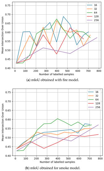
Figure 8.
Evolution of segmentation metric mIoU for fire and smoke AL models with different acquisition sizes and a fixed warmstart size (1% of the total dataset) in the test set (experiment C.2).
6. Conclusions
The task of performing fire and smoke detection is not trivial. Our proposed approach uses a CNN, in conjunction with AL methods, to create an image classification model that provides predictions of the presence of fire and/or smoke while making use of datasets with image-level labels. An uncertainty AL method was used, where an oracle queries the most uncertain data samples (and therefore, the most informative samples to the model). Linked to this system is a weakly supervised approach using CAM and CRF. CAM retrieves the most relevant image features used on the prediction of a given sample, producing a heatmap of the image, and CRF performs postprocessing on this heatmap by taking into account the contextual information neighboring the heatmap. With this model, it was possible to produce reliable image detections of fire and smoke.
From the results of this work, when running an AL model, specifically in the case of fire and smoke detection, if the goal of the user is to achieve the best results, with the minimal number of samples possible, a smaller warmstart size and acquisition size should be set. Choosing small warmstart sizes and acquisition sizes has two goals: increasing the number of AL rounds and allowing for the algorithm to select the most informative samples earlier. Both these factors are closely linked with the ability of the model to obtain the best results with a minimal number of samples. By lowering the acquisition size, the number of AL rounds is increased. By lowering the warmstart size, the model has the ability to select the most informative samples as early as possible. The drawback of these options is that the training time will become considerably higher from the additional training rounds.
Despite this, our model presented some limitations, which will be listed next. We will also indicate some future work to overcome those limitations. First, the computational resources involved in the training of an AL model are significantly higher than a non-AL model. There are solutions to partially mitigate this constraint, by either increasing the number of samples in which the model is initially trained (warmstart size) or by increasing the acquisition size (number of samples that are queried per AL round). However, by increasing either of these values, we are increasing the number of labeled samples needed to achieve the optimal model. The second main constraint is that evaluating how a model will behave when performing segmentation is not trivial. For example, models that were trained with a similar number of AL rounds and had identical results often performed quite differently in the segmentation phase. This can be solved by making sure that the training of the model is stopped whenever the training achieves the optimal model (best results, with the least number of samples). The third constraint is that determining where the optimal training state is to locate the moment when the training should be stopped usually involves training the model several times and gathering information about how the training, validation, and test results vary in order to discover where this point is situated.
As far as we know, this work is the first one to implement an AL methodology in the context of fire and smoke detection. Adding to the previous point, our work is also the first one to implement two different approaches designed to remove the complexities of the dataset gathering process: weakly supervised learning and active learning, in this area of research. On a related note, in terms of fire and smoke detection, we substantially minimize the dataset needs by making use of two approaches designed for this purpose. On the one hand, we only use image-level labels by the use of WSS; on the other hand, by using AL, we reduce the number of samples needed to achieve the same results as non-AL methodologies. Having said this, we prove the viability of the implementations of our work in this field of research.
Nevertheless, there are two main avenues of future work to be developed. The first line of future work is improvement of different areas in the proposed method. For instance, in the classification phase, the implementation of the original work of DEAL could be revised once again to study the possibility of total implementation and to additionally improve the accuracy of the results. To improve the training time, since we are running successive AL rounds, the substitution of the CNN type used in this work (VGG) with a faster working CNN could be beneficial. In the segmentation phase, two possibilities could be considered. The first one is to upgrade the CAM method to Grad-CAM to better extract the relevant image features. The second one would be to study the implementation of our approach with dedicated AL segmentation methods, thus combining semisupervised methods with AL. The second line of future work is the usage of AL with state-of-the-art segmentation methods. In particular, by using a dedicated AL segmentation method, the use of interactive learning in the area of fire and smoke detection could be developed.
Author Contributions
Conceptualization, T.M., A.B. and G.C.; methodology, T.M., A.B. and G.C.; software, T.M.; validation, T.M., A.B. and G.C.; formal analysis, T.M., A.B. and G.C.; investigation, T.M., A.B. and G.C.; resources, T.M., A.B. and G.C.; writing—original draft preparation, T.M.; writing—review and editing, A.B. and G.C.; visualization, T.M., A.B. and G.C.; supervision, A.B. and G.C.; project administration, A.B.; funding acquisition, A.B. and G.C. All authors have read and agreed to the published version of the manuscript.
Funding
This research was supported by the project FIREFRONT with the reference PCIF/SSI/0096/2017, FCT Projects LARSyS UIDBP/50009/2020, and LA/P/0083/2020.
Data Availability Statement
The datasets used in this study are available at https://cfdb.univcorse.fr/ (accessed on 19 August 2023) [7], http://wildfire.fesb.hr/ (accessed on 19 August 2023) [33], and http://smoke.ustc.edu.cn/datasets.htm (accessed on 19 August 2023) [34]. The considered active learning method is available at https://github.com/trmarto/fire-smoke-AL.git (accessed on 6 February 2023).
Acknowledgments
The authors would like to thank all the partners in the FIREFRONT project that allowed data to be gathered and provided ideas and discussions that led to this work.
Conflicts of Interest
The authors declare no conflict of interest.
Abbreviations
The following abbreviations are used in this manuscript:
| AL | active learning |
| CAM | class activation mapping |
| CEAL | cost-effective active learning |
| CNN | convolutional neural network |
| CRF | conditional random fields |
| DEAL | deep evidential active learning |
| GAN | generative adversarial network |
| GAP | global average pooling |
| GT | ground truth |
| IoU | intersection over union |
| mIoU | mean intersection over union |
| RGB | red green blue |
| R-CNN | region-based convolutional neural network |
| UAV | unmanned aerial vehicle |
| VGG | visual geometry group |
| WSL | weakly supervised learning |
| WSS | weakly supervised segmentation |
References
- Instituto da Conservação da Natureza e das Florestas (ICNF). Incêndios Rurais e área Ardida-Continente; ICNF: Lisbon, Portugal, 2021. [Google Scholar]
- Instituto da Conservação da Natureza e das Florestas. Relatório anual de áreas ardidas e incêndios florestais em Portugal Continental; Technical Report; Ministério do Ambiente: Lisbon, Portugal, 2016.
- Hodgetts, H.M.; Vachon, F.; Chamberland, C.; Tremblay, S. See No Evil: Cognitive Challenges of Security Surveillance and Monitoring. J. Appl. Res. Mem. Cogn. 2017, 6, 230–243. [Google Scholar] [CrossRef]
- Lin, T.Y.; Maire, M.; Belongie, S.; Hays, J.; Perona, P.; Ramanan, D.; Dollár, P.; Zitnick, C.L. Microsoft coco: Common objects in context. In Proceedings of the Computer Vision–ECCV 2014: 13th European Conference, Zurich, Switzerland, 6–12 September 2014; pp. 740–755. [Google Scholar]
- Santana, B.; Cherif, E.K.; Bernardino, A.; Ribeiro, R. Real-Time Georeferencing of Fire Front Aerial Images Using Iterative Ray-Tracing and the Bearings-Range Extended Kalman Filter. Sensors 2022, 22, 1150. [Google Scholar] [CrossRef] [PubMed]
- Zhang, Q.X.; Lin, G.H.; Zhang, Y.M.; Xu, G.; Wang, J.J. Wildland forest fire smoke detection based on faster R-CNN using synthetic smoke images. Procedia Eng. 2018, 211, 441–446. [Google Scholar] [CrossRef]
- Toulouse, T.; Rossi, L.; Campana, A.; Celik, T.; Akhloufi, M.A. Computer vision for wildfire research: An evolving image dataset for processing and analysis. Fire Saf. J. 2017, 92, 188–194. [Google Scholar] [CrossRef]
- Kotaridis, I.; Lazaridou, M. Remote sensing image segmentation advances: A meta-analysis. ISPRS J. Photogramm. Remote. Sens. 2021, 173, 309–322. [Google Scholar] [CrossRef]
- Settles, B. Active Learning Literature Survey; Computer Sciences Technical Report 1648; University of Wisconsin–Madison: Madison, WI, USA, 2009. [Google Scholar]
- Breck, E.; Polyzotis, N.; Roy, S.; Whang, S.; Zinkevich, M. Data Validation for Machine Learning. In Proceedings of the MLSys, Palo Alto, CA, USA, 31 March–2 April 2019. [Google Scholar]
- Ros, G.; Sellart, L.; Materzynska, J.; Vazquez, D.; Lopez, A.M. The synthia dataset: A large collection of synthetic images for semantic segmentation of urban scenes. In Proceedings of the IEEE Conference on Computer Vision and Pattern Recognition, Las Vegas, NV, USA, 27–30 June 2016; pp. 3234–3243. [Google Scholar]
- Xu, S.; Chen, Y.; Ma, C.; Yue, X. Deep evidential fusion network for medical image classification. Int. J. Approx. Reason. 2022, 150, 188–198. [Google Scholar] [CrossRef]
- Aklilu, J.; Yeung, S. ALGES: Active learning with gradient embeddings for semantic segmentation of laparoscopic surgical images. In Proceedings of the Machine Learning for Healthcare Conference—PMLR, Durham, NC, USA, 5–6 August 2022; pp. 892–911. [Google Scholar]
- Wörmann, J.; Bogdoll, D.; Bührle, E.; Chen, H.; Chuo, E.F.; Cvejoski, K.; van Elst, L.; Gottschall, P.; Griesche, S.; Hellert, C.; et al. Knowledge augmented machine learning with applications in autonomous driving: A survey. arXiv 2022, arXiv:2205.04712. [Google Scholar]
- Khan, S.; Muhammad, K.; Hussain, T.; Del Ser, J.; Cuzzolin, F.; Bhattacharyya, S.; Akhtar, Z.; de Albuquerque, V.H.C. Deepsmoke: Deep learning model for smoke detection and segmentation in outdoor environments. Expert Syst. Appl. 2021, 182, 115125. [Google Scholar] [CrossRef]
- Luo, Y.; Zhao, L.; Liu, P.; Huang, D. Fire smoke detection algorithm based on motion characteristic and convolutional neural networks. Multimed. Tools Appl. 2018, 77, 15075–15092. [Google Scholar] [CrossRef]
- Amaral, B.; Bernardino, A.; Barata, C. Fire and Smoke Detection in Aerial Images. Master’s Thesis, Instituto Superior Técnico, Lisbon, Portugal, 2021. [Google Scholar]
- Fernandes, S. Detecção de Incêndios Florestais Através da Aprendizagem Auto-Supervisionada. Master’s Thesis, Instituto Superior Técnico, Lisbon, Portugal, 2021. [Google Scholar]
- Kuhlmann, L. Semi-Supervised Semantic Segmentation of Smoke and Fire from Airborne Images with Generative Adversarial Networks to Support Firefighting Actions. Master’s Thesis, HTW Berlim, Berlin, Germany, 2021. [Google Scholar]
- Namozov, A.; Im Cho, Y. An efficient deep learning algorithm for fire and smoke detection with limited data. Adv. Electr. Comput. Eng. 2018, 18, 121–128. [Google Scholar] [CrossRef]
- Hemmer, P.; Kühl, N.; Schöffer, J. Deal: Deep evidential active learning for image classification. In Deep Learning Applications; Springer: Singapore, 2022; Volume 3, pp. 171–192. [Google Scholar]
- LeCun, Y.; Bottou, L.; Bengio, Y.; Haffner, P. Gradient-based learning applied to document recognition. Proc. IEEE 1998, 86, 2278–2324. [Google Scholar] [CrossRef]
- Krizhevsky, A.; Hinton, G. Learning Multiple Layers of Features from Tiny Images; Technical Report 0; University of Toronto: Toronto, ON, Canada, 2009. [Google Scholar]
- Kermany, D.S.; Goldbaum, M.; Cai, W.; Valentim, C.C.; Liang, H.; Baxter, S.L.; McKeown, A.; Yang, G.; Wu, X.; Yan, F.; et al. Identifying medical diagnoses and treatable diseases by image-based deep learning. Cell 2018, 172, 1122–1131. [Google Scholar] [CrossRef]
- Zhou, B.; Khosla, A.; Lapedriza, A.; Oliva, A.; Torralba, A. Learning deep features for discriminative localization. In Proceedings of the IEEE Conference on Computer Vision and Pattern Recognition, Las Vegas, NV, USA, 27–30 June 2016; pp. 2921–2929. [Google Scholar]
- Chen, L.C.; Papandreou, G.; Kokkinos, I.; Murphy, K.; Yuille, A.L. Deeplab: Semantic image segmentation with deep convolutional nets, atrous convolution, and fully connected crfs. IEEE Trans. Pattern Anal. Mach. Intell. 2017, 40, 834–848. [Google Scholar] [CrossRef]
- Shimoda, W.; Yanai, K. Distinct class-specific saliency maps for weakly supervised semantic segmentation. In Proceedings of the European Conference on Computer Vision, Amsterdam, The Netherlands, 11–14 October 2016; Springer: Cham, Switzerland; pp. 218–234.
- Wang, K.; Zhang, D.; Li, Y.; Zhang, R.; Lin, L. Cost-effective active learning for deep image classification. IEEE Trans. Circuits Syst. Video Technol. 2016, 27, 2591–2600. [Google Scholar] [CrossRef]
- Krstinic, D.; Jakovcevic, T. Image Database. 2010. Available online: http://wildfire.fesb.hr/ (accessed on 24 February 2023).
- Zhang, Q. Research Webpage about Smoke Detection for Fire Alarm: Datasets. Available online: http://smoke.ustc.edu.cn/datasets.htm (accessed on 24 February 2023).
- Krizhevsky, A.; Sutskever, I.; Hinton, G.E. Imagenet classification with deep convolutional neural networks. Commun. ACM 2017, 60, 84–90. [Google Scholar] [CrossRef]
- Glorot, X.; Bengio, Y. Understanding the difficulty of training deep feedforward neural networks. In Proceedings of the Thirteenth International Conference on Artificial Intelligence and Statistics, Chia Laguna Resort, Sardinia, Italy, 13–15 May 2010; Volume 9, pp. 249–256. [Google Scholar]
- Bugarić, M.; Jakovčević, T.; Stipaničev, D. Adaptive estimation of visual smoke detection parameters based on spatial data and fire risk index. Comput. Vis. Image Underst. 2014, 118, 184–196. [Google Scholar] [CrossRef]
- Xu, G.; Zhang, Y.; Zhang, Q.; Lin, G.; Wang, J. Deep domain adaptation based video smoke detection using synthetic smoke images. Fire Saf. J. 2017, 93, 53–59. [Google Scholar] [CrossRef]
Disclaimer/Publisher’s Note: The statements, opinions and data contained in all publications are solely those of the individual author(s) and contributor(s) and not of MDPI and/or the editor(s). MDPI and/or the editor(s) disclaim responsibility for any injury to people or property resulting from any ideas, methods, instructions or products referred to in the content. |
© 2023 by the authors. Licensee MDPI, Basel, Switzerland. This article is an open access article distributed under the terms and conditions of the Creative Commons Attribution (CC BY) license (https://creativecommons.org/licenses/by/4.0/).

