Monitoring Waterlogging Damage of Winter Wheat Based on HYDRUS-1D and WOFOST Coupled Model and Assimilated Soil Moisture Data of Remote Sensing

Abstract

Waterlogging harms winter wheat growth. To enable accurate monitoring of agricultural waterlogging, this paper conducts a winter wheat waterlogging monitoring study using multi-source data in Guzhen County, Anhui Province, China. The hydrological model HYDRUS-1D is coupled with the crop growth model WOFOST, and the Ensemble Kalman Filter is used to assimilate Sentinel-1 inversion soil moisture data. According to the precision and continuity of soil moisture, the damage of winter wheat waterlogging were obtained. The experimental results show that the accuracy of the soil moisture is improved after data assimilation compared with that before data assimilation, and the Nash–Sutcliffe efficiency (NSE) of the simulated soil moisture values at three monitoring sites increased from 0.528, 0.541 and 0.575 to 0.752, 0.692 and 0.731, respectively. A new waterlogging identification criterion has been proposed based on the growth periods and probability distribution of soil moisture. The proportion, calculated from this identification criterion, of the waterlogging wheat farmland in total farmland shows a high correlation with the yield reduction rate. The correlation coefficient of the waterlogging farmland proportion and the yield reduction rate in 11 towns of Guzhen County reaches 0.78. Through the synchronization of geography, agriculture and meteorology, the framework shows great potential in waterlogging monitoring.

1. Introduction

The continuous precipitation or low location of the winter wheat growing area results in excessive soil moisture. A waterlogged winter wheat root system is deprived of oxygen for a prolonged period, negatively affecting the growth and development of the winter wheat, resulting in reduced food production [1,2]. Around 10–15% of the global wheat acreage is estimated to be damaged [3]. Accurately assessing the degree of winter wheat damage and the risk associated with the damage is essential to improving the capacity to control winter wheat damage [4,5].

The traditional method of monitoring waterlogging damage is to monitor meteorological data from ground-based weather stations and then use these data to indirectly determine the extent of the damage. The widely used meteorological data for waterlogging damage detection include the Standardized Precipitation Index (SPI), the Rainfall Anomaly Index (RAI) and the cumulative wetness index, which combines precipitation and evapotranspiration information [6]. Traditional methods of monitoring and assessing agricultural hazards are time-consuming, subjective and challenging to monitor over large areas. Rapid developments in remote sensing, geoinformation and global positioning technologies have created new monitoring, warning and assessment methods for agro-meteorological hazards. For example, the soil moisture can be inverted from remote sensing, and then the inverted soil moisture data can be used for monitoring waterlogging damage. Taking advantage of the fact that the reflectance of water in the visible and near-infrared varies greatly, the use of optical remote sensing can be realised to invert surface soil moisture [7]. The shortcoming of current optical remote sensing technology is that it cannot be observed in cloudy weather. Since heavy rainfall often causes waterlogging, this constraint affects the ability to continuously monitor waterlogging [8]. In addition, visible and near-infrared light cannot penetrate the dense vegetation canopy to provide information about the soil [9].

Unlike visible and near-infrared data, microwave remote sensing is less affected by the atmosphere and can be observed on cloudy days [10]. There are great differences in dielectric constant between wet soil and dry soil. Therefore, the microwave technique is a good method for measuring soil moisture. The difficulty with passive microwave detection of waterlogging is its poor resolution [11]. The use of active microwave observations can provide information about waterlogging with a high spatial resolution. For example, Synthetic Aperture Radar (SAR) can detect surface soil moisture under vegetation [12]. Since waterlogging is a situation where crops are affected by excessive soil moisture over several consecutive days, high temporal-resolution soil-moisture data is required to observe waterlogging [13]. However, due to the long re-entry period of SAR, continuous soil moisture data cannot be obtained. The space and time resolution of the existing satellite products has restricted the feasibility of waterlogging monitoring in irrigation.

In recent years, combining hydrological models and crop growth models can simulate continuous soil moisture [14,15,16]. A hydrological model is a mathematical abstraction of the natural hydrological system and is currently the basic tool for hydrological research. Hydrological models include at least surface soil moisture and groundwater components. Currently, the main hydrological models include the HBV model [17], TOPMODEL model [18], SWAT model [19], VIC model [20], DHSVM model [21] and HYDRUS-1D model [22]. A crop growth model is a tool that estimates crop growth and yield based on weather conditions, soil conditions and field management practices. Several kinds of models have been developed around the world in recent decades. The main ones include the WOFOST model [23], the COTGROW model [24], the CERES-Wheat model [25] and the DSSAT models [26]. Crop growth modelling simulates the growth and development of crops, but it slightly simplifies the simulation of water movement and hydrological balance. Water balance based on the hydrological flow equation can be accurately simulated by a hydrological model. However, hydrologic models cannot simulate crop growth and development processes. Therefore, it is necessary to combine the advantages of the crop growth model with the hydrological model to achieve the goal of accurately simulating soil moisture. Zhou et al. coupled the HYDRUS-1D model with the WOFOST model for wheat cultivation and irrigation simulation to optimize irrigation, and the coupled model simulates wheat production under variable moisture conditions [14]. Li et al. coupled the SHAW and WOFOST models to investigate the water, carbon and energy balance of irrigated maize [16]. Shelia et al. coupled HYDRUS-1D and DSSAT models to simulate soil moisture dynamics in a soil–vegetation–atmosphere system [15]. The existing studies provide support for coupling crop growth models with hydrological models and also create the possibility of applying the coupled models in monitoring waterlogging damage.

In this paper, inverted soil moisture data are obtained by Sentinel-1, and soil moisture simulation data are obtained by the HYDRUS-1D and WOFOST coupled model, and the two kinds of data are assimilated based on an Ensemble Kalman Filter algorithm to obtain the final soil moisture values. A new waterlogging identification criterion has been proposed based on the growth periods and probability distribution of soil moisture. The proposed criterion can obtain the distribution of the risk and the grade of waterlogging damage. The new algorithm has been verified to have some practical benefits through comparative analysis with yield reduction rate data.

2. Research Area and Data

2.1. Research Area

In the northern part of Anhui Province of China, Guzhen County is located between 33°10′ and 33°30′ N latitude and 117°02′ and 117°36′ E longitude. From east to west, it is about 47 km wide, and from north to south, it is about 51 km long. The overall area is approximately 1363 square kilometers. Figure 1 illustrates the geographical location of the study area. The study area is a significant winter wheat planting area. Precipitation data from previous years show that winter wheat in the region receives less precipitation during the pre-growth period, with the least occurring from December to January and the most occurring from April to May. The average precipitation days from October to January of the next year of the study area are less than those in the later months. It indicates that the precipitation intensity in the late growth period is much larger than that in the early growth period for winter wheat.

2.2. Research Data

2.2.1. Auxiliary Data

• Topographic and soil data

DEM data, soil types, feature types, river network data, flow data and meteorological data are applied in the HYDRUS-1D and WOFOST coupled model. SRTM digital elevation data (DEM) at 30 m resolution is available from the Geospatial Data Cloud website (http://www.gscloud.cn/, accessed on 10 December 2022). The geographic data are downloaded from the National Basic Geographic Information System database (http://nfgis.nsdi.gov.cn/asp/userinfo.asp, accessed on 22 June 2023).

The daily value dataset of Chinese ground climate information is derived from the National Meteorological Science Data Center (http://data.cma.cn/, accessed on 11 December 2022). Information on soil texture is provided by the International Soil Reference and Information Center (https://www.isric.org/, accessed on 20 December 2022). Winter wheat planting area is derived from the Chinese Academy of Science Discipline Data Center for Ecosystem (http://nesdc.org.cn/, accessed on 20 December 2022).

• Farmland Information Collection Sites

Obtaining complete and detailed disaster records on a large scale is difficult, however, hydrological observation data are an essential source of information for monitoring the impact of the damage. From 10 May 2017 to 27 May 2018, three automatic farmland information collection sites were set up in the study area (shown in Figure 1). The stations observe the following parameters: temperature, humidity, total radiation, photosynthetically active radiation, wind direction and wind speed. Soil moisture is monitored using a Decagon EC50 automatic soil moisture monitor, which is buried at a depth of 0.05 m. All instruments are set to automatically record once per hour. Three devices are installed in the study area at Location 1 (33°19′25″ N, 117°11′13″ E), Location 2 (33°26′11″ N, 117°16′39″ E) and Location 3 (33°16′48″ N, 117°23′11″ E). The specific positions of the instruments are shown in Figure 1c.

2.2.2. Remote Sensing Satellite Data

Remote sensing data were collected from 11 October 2017 to 27 May 2018 to monitor the growth of winter wheat. It consisted mainly of Sentinel-1 data and Sentinel-2 medium-resolution multispectral optical data. Sentinel-2 data are used to calculate vegetation indices. In addition, 19 Sentinel-1 data are used to invert the soil moisture in the study area. Parameters of Sentinel-1 are presented in

Table 1. Parameters for Sentinel-1 used in this paper.

Parameters	Sentinel-1
Product type	Ground Range Detected (GRDH)
First acquisition	11 October 2017
Last acquisition	27 May 2018
Pass direction	Ascending
Polarization mode	VV + VH
Incidence angle	30.63–46.07
Wavelength	5.5 (c-band)
Range spacing	2.33
Azimuth spacing	13.92
spatial resolution	5 m × 20 m

and specific information for Sentinel-2 is shown in

Table 2. Specific information for Sentinel-2 used in this paper.

Sentinel-2 Band	Central Wavelength	Resolution (m)
B2-Blue	496.6	10
B3-Green	560	10
B4-Red	664.5	10
B8-NIR	835.1	10
B5-Red-edge 1	703.9	20
B6-Red-edge 2	740.2	20
B7-Red-edge 3	782.5	20
B8A-NIR narrow	864.8	10
B11-SWIR1	1613.7	20
B12-SWIR2	2202.4	20

.

3. Research Methodology

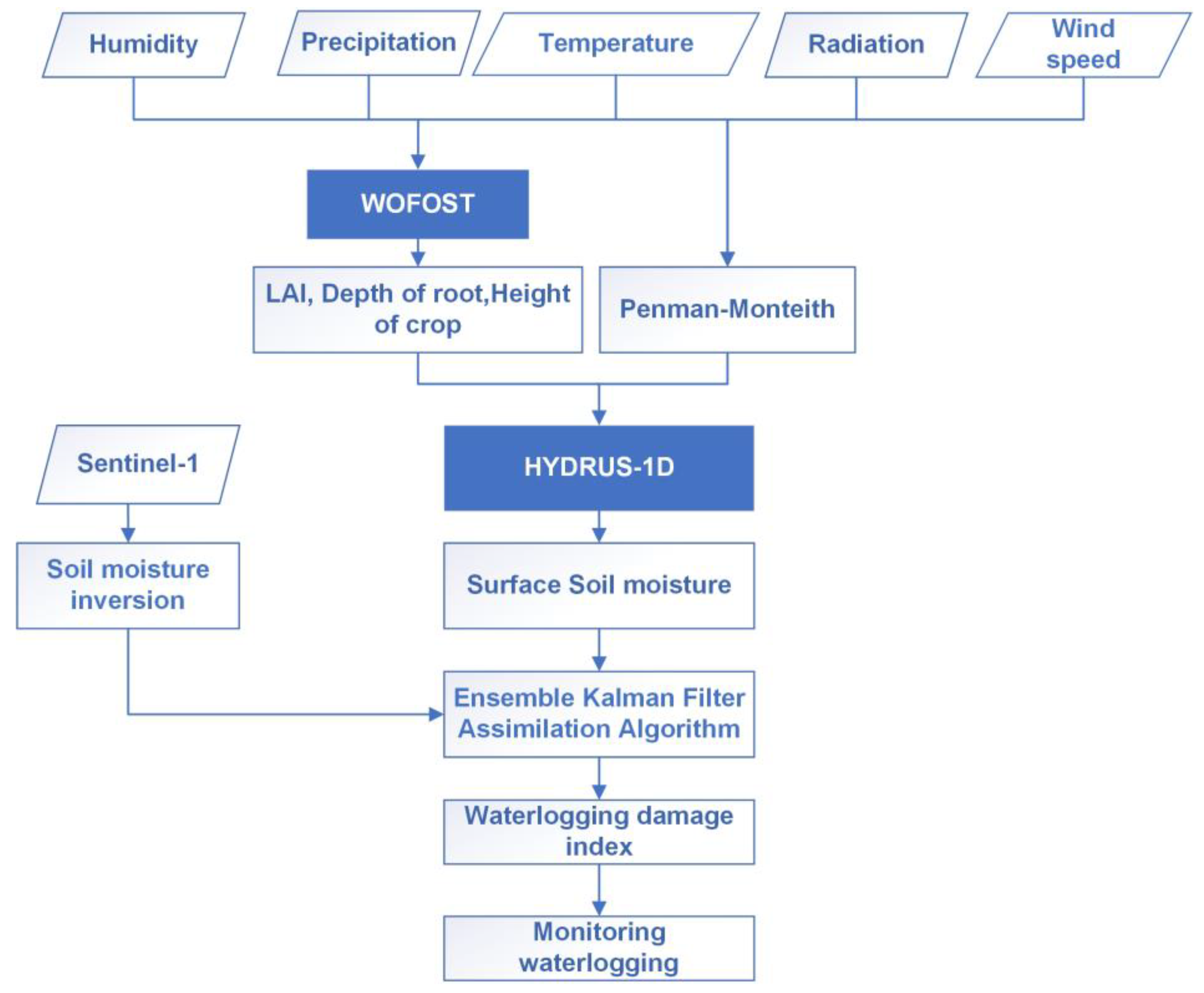
This paper proposed a systematic method for winter wheat damage monitoring using multi-source data, the structure of the proposed method is shown in Figure 2. The soil moisture observation value is inverted by Sentinel-1, the soil moisture simulation value is obtained by the HYDRUS-1D and WOFOST coupled model, and the soil moisture data of the winter wheat cover area in Guzhen County is calculated by the Ensemble Kalman Filter assimilation method. Finally, a new waterlogging identification criterion has been proposed based on the growth periods and probability distribution of soil moisture. The identification criterion has been used to monitor and assess the risk of waterlogging damage in the study area.

3.1. Crop Growth Model

The WOFOST model can be used to quantitatively analyze the growth and output of the plants. It is a potential process-based mechanical model that simulates the basic processes of plant growth, including photosynthesis, respiratory and environmental conditions like soil moisture, climatic and fertilizer use. In this paper, we can simulate the influence of climate, soil and operation on plants. The WOFOST model has been widely used for many climatic and management conditions around the world. The program is relatively simple, but does not reflect well the pattern of soil moisture change during crop growth. Specific pattern descriptions for this code can be found in van Ittersum et al. [27].

3.2. Hydrological Model

The hydrological model HYDRUS-1D solves the Richards equation for variably saturated flows and the convection–dispersion equations for heat and solute transport [28]. In particular, a channel coefficient that reflects the water lifted by the roots of the plant has been included in the hydrodynamic model. The hydrodynamic model is capable of dealing with two forms of porosity, one of which is fluid and the other non-fluid; it can also be considered to contain two different permeable fluids, one matric and one microporous. The heat and solute transport equations in the model take into account transport due to the conduction and convection of flowing water. The HYDRUS-1D model simulates processes such as vertical movement of soil moisture, energy balance, potential evapotranspiration and water lifting by the crop roots.

A modified one-dimensional Richards equation was proposed for simulation of vertical flow in non-saturated region. The numerical solution of the equation is discretized vertically using the Galerkin Finite Elements method and, for the time scale solution, is calculated using an implicit difference format [29]:

$$\frac{{\partial }_{\theta }}{{\partial }_t}=\frac{\partial }{{\partial }_x}\left[K\left(\frac{{\partial }_h}{{\partial }_x}+\cos \alpha \right)\right]-S$$

(1)

where $h$ is the water pressure head (or soil moisture potential) (cm); $\theta$ is the volumetric water content of the soil (cm²/cm³); $t$ is the time interval, which in this study is measured in days (d); $x$ is the vertical depth, which is positive downwards (cm); $S$ is the water extracted by the root system (cm³$\cdot$cm⁻³$\cdot$d⁻¹), and it defines water extracted from the soil by the crop roots in unit time and physical volume; $\alpha$ is the angle between the direction of flow and the vertical direction ($\alpha$ = 0 for vertical flow, 90° for horizontal flow and 0° < $\alpha$ < 90° for inclined flow); and $K$ is the unsaturated hydraulic conductivity (cm/d), calculated using the van Genuchten simulation equation as:

$$K(h)=K_s{S}_e^l{\left[1-{\left(1-S_e^{1/m}\right)}^m\right]}^2\hspace{1em}h<0$$

(2)

$$S_e=\frac{\theta -{\theta }_r}{{\theta }_s-{\theta }_r}$$

(3)

$$\theta (h)=\left\{\begin{array}{c}{\theta }_r+\frac{{\theta }_s - {\theta }_r}{{\left[1+|\alpha h{|}^n\right]}^m}\begin{array}{cc}& \end{array}h<0\\ {\theta }_s\begin{array}{cccc}& & & \begin{array}{cc}\begin{array}{cc}& \end{array}& \end{array}\end{array}h\ge 0\end{array}\right.$$

(4)

where $K_s$ is the saturated hydraulic conductivity (cm/d); $S_e$ is the dimensionless effective moisture content; $S_e^l$ is the effective saturation (cm³/cm³); ${\theta }_s$ is the saturated hydraulic conductivity (cm³/cm³); ${\theta }_r$ is the residual water content (cm³/cm³); $\alpha$, $n$ and $m$ are the empirical parameters of the van Genuchten model [30], respectively; n is the porosity distribution parameter; $m=1-\frac{1}{n}\left(n>1\right)$; and $l$ is the pore connectivity parameter.

In the HYDRUS-1D model, Feddes model is used to calculate the rate of water lifting by the root system, calculated as:

$$S(h)=\alpha (h)S_p$$

(5)

where $\alpha (h)$ is a dimensionless water stress response function (0 ≤ $\alpha (h)$ ≤ 1) to describe the degree of decline in root water extraction due to water stress; $S_p$ is the potential rate of water lifting (d⁻¹). The water stress response function $\alpha (h)$ is usually expressed as:

$$\alpha (h)=\left\{\begin{array}{cc}0& h\le h_4\\ \left(h-h_4\right)/\left(h_3-h_4\right)& h_4<h\le h_3\\ 1& h_3<h\le h_2\\ \left(h-h_1\right)/\left(h_2-h_1\right)& h_2<h\le h_1\\ 0& h>h_1\end{array}\right.$$

(6)

$$S_p=b(x)T_p$$

(7)

$$b(x)=\frac{b^{\prime }(x)}{{\int }_0^{L_R}{b}^{\prime }(x)dx}$$

(8)

where $h_1$, $h_2$, $h_3$ and $h_4$ are threshold parameters for root water extraction, $h_1$ is the anaerobic point and $h_4$ is the wilting point water potential. When the water potential is between $h_2$ and $h_3$, the crop root water extraction rate is equal to the potential root water extraction rate and reaches the maximum; when the water potential $h\le h_4$ or $h>h_1$, the crop root water extraction is equal to 0; when $h_4<h\le h_3$, root water extraction tends to increase linearly; and when $h_2<h\le h_1$, root water extraction tends to decrease linearly. $T_p$ is the potential transpiration rate (cm/d). $b(x)$ is the root distribution function, which usually represents the temporal dynamic distribution of the plant root system in the vertical direction of the soil and is generally obtained from actual observations or models combined with empirical simulations. $L_R$ is the root depth (cm).

The HYDRUS-1D model uses the potential transpiration of the reference crop as the main part of plant water consumption, calculated as shown in the equations:

$$T_p=E{T}_0\left(1-e^{-k\mathrm{LAI}}\right)$$

(9)

$$E_p=E{T}_0{e}^{-k\mathrm{LAI}}$$

(10)

where $E_p$ is the potential soil evapotranspiration (cm/d); $k$ is the attenuation coefficient of the plant canopy to solar radiation, a dimensionless function of solar altitude angle, plant distribution and leaf arrangement, usually taking a value of 0.4 for winter wheat; and $E{T}_0$ is the reference Crop evapotranspiration, calculated by the Penman–Monteith formula as [31]:

$$E{T}_0=\frac{0.408\mathsf{\Delta }\left(R_n-G\right)+\gamma \frac{900}{T+273}{U}_2\left(e_s-e_a\right)}{\mathsf{\Delta }+\gamma \left(1+0.34U_2\right)}$$

(11)

where $\mathsf{\Delta }$ is calculated from the fitted proportional relationship between saturated water vapor pressure and air temperature, i.e., the slope of the two calculations (kPa/°C); $R_n$ is the net radiation received by the vegetation canopy surface (MJ/(m²$\cdot$d)); $G$ is the soil surface heat flux (MJ/(m²$\cdot$d)); $T$ is the daily average air temperature (°C); and $U_2$ is the 2 m height wind speed (m/s). $e_s$ is the near-surface saturated water vapor pressure (kPa); $e_a$ is the actual near-surface water vapor pressure (kPa); and $\gamma$ is the hygrometer constant (kPa/°C).

3.3. Couple Model

The Richards equation in the HYDRUS-1D model simulates the dynamic characteristics of soil moisture. The ratio of actual to potential transpiration simulated using the HYDRUS-1D model characterizes the effect of soil moisture stress on crop production, i.e., the water stress response factor.The WOFOST model simulates CO₂ assimilation (photosynthesis) and respiration in the crop, and then assimilates are partitioned to the various organs of the crop to maintain the changes in the crop parameters such as the crop leaf area index (LAI) and the length of the root system. Based on the respective advantages of the hydrological model and the crop growth model, the potential evapotranspiration and root lift were mainly calculated in the hydrological model in the study and transferred to the crop growth model, where the crop growth process was simulated in the crop growth model. In the simulation of the crop growth process, the state variables computed include covariates such as leaf area index, root depth, and vegetation height. The crop growth model passes the simulated state variables to the hydrological model. The coupling between the crop growth model and the hydrological model is realized by completing the day-by-day dynamic interaction of parameters between the above models. The framework of the coupled model is shown in Figure 3.

The HYDRUS-1D and WOFOST models can be operated daily in order to realize temporal consistency among the models. The coupled model can be divided into the following steps to address the characteristics of the study area:

(1)

The input terms in the HYDRUS-1D model included irrigation and precipitation, daily net radiation, daily maximum and minimum temperatures, daily wind speed and daily relative humidity.

(2)

The HYDRUS-1D model is applied to compute the potential evapotranspiration and transpiration by a combination of Penman–Monteith approach.

(3)

In HYDRUS-1D, water absorption is computed from Feds’ equation [32].

(4)

The HYDRUS-1D model is applied to calculate the soil moisture, the water level and the depth of the ground water.

(5)

Due to the fact that the majority of soil moisture absorption is taken up by plant transpiration, it is assumed that the amount of soil moisture absorbed per day is equal to that of actual evaporation. Furthermore, a proxy for water pressure is taken as a proxy for the level of water-stress in the case of Feddas, based on Feddas, and possible transpiration using the Penman–Monteith approach [33].

(6)

Calculation of the real day CO₂ absorption per day shall be carried out by multiplying the CO₂ absorption of the entire potential per day of harvest using a WOFOST model using a water-stress factor. Then, the amount of carbs distributed among different portions of the harvest is computed using a WOFOST model.

(7)

Subsequently, the vegetation parameters, based on a WOFOST model, more specificly root depth, crop altitude and LAI, will be used as an input for HYDRUS-1D.

3.4. Remote Sensing Soil Moisture Inversion Method

The Sentinel-1 data were applied to invert the soil moisture. The Ulaby method is used to eliminate the effect of the incident angle on the backscattering coefficient to normalize the backscattering coefficient, which is calculated as [34]:

$${\sigma }_{{\theta }_{ref}}^0={\sigma }_{\theta }^0\frac{{\cos }^2{\theta }_{ref}}{{\cos }^2\theta }$$

(12)

where ${\sigma }_{{\theta }_{ref}}^0$ is the standard value of the backscattering coefficient; ${\sigma }_{\theta }^0$ is the Sentinel-1A Sar data backscatter coefficient; ${\theta }_{ref}$ is the standard incidence angle; and $\theta$ is the incidence angle of Sentinel-1.

The water-cloud model is adopted to remove the influence of the surface vegetation on the backscatter coefficient [35]. The calculation formula of the water-cloud model is

$${\sigma }_{{\theta }_{ref}}^0={\theta }_{veg}^0+{\tau }^2{\sigma }_{soil}^0$$

(13)

$${\tau }^2=\exp \left(-\frac{2B{V}_2}{\cos \theta }\right)$$

(14)

$${\sigma }_{\mathrm{veg}}^0=A{V}_1\cos \theta \left(1-{\tau }^2\right)$$

(15)

where ${\sigma }_{soil}^0$ is the backscatter coefficient of the soil surface layer, ${\sigma }_{\mathrm{veg}}^0$ is the vegetation-generated backscatter coefficient, ${\tau }^2$ is the two-way attenuation coefficient, $V_1$ denotes the scattering characteristics of the vegetation, $V_2$ denotes the attenuation characteristics of the vegetation, $A$ is the coefficient related to vegetation density, and B is a coefficient related to crop type. We consider V₁ = V₂ = NDVI, since a number of studies have demonstrated that NDVI can be calculated with high precision as a single plant description [36]. The NDVI indices for each period in the study were calculated from the Sentinel-2 data.

This paper uses the Alpha approximation model for soil moisture inversion [37]. For SAR images taken at $T_1$ and $T_2$, it is possible to estimate the proportion of the radar backscatter coeffient obtained in those two times as a proportion of earth permittivity, an incident angle of radar and a polarimetric square, provided that the surface roughness is maintained at a constant value over this period of time. It can be expressed as:

$$\frac{{\sigma }_{0,\mathrm{pp}}^{T_2}}{{\sigma }_{0,\mathrm{pp}}^{T_1}}\approx {\left|\frac{{\alpha }_{\mathrm{pp}}^{T_2}\left(\theta ,{\epsilon }_s\right)}{{\alpha }_{\mathrm{pp}}^{T_1}\left(\theta ,{\epsilon }_s\right)}\right|}^2$$

(16)

where σ₀ is the radar backscatter coefficient; $\theta$ is the radar incidence angle; ${\epsilon }_s$ is the relative permittivity of the soil; $T_1$ and $T_2$ are the times of radar data acquisition; ${\alpha }_{\mathrm{pp}}^{}$ is the amplitude of polarization, which is a function of the angle of radar incidence and the soil dielectric constant. $PP$ indicates the polarization mode, either $HH$ or $VV$.

This paper uses data from the VV polarization of sentinel-1, which is adopted to describe the scattering from the surface, and the polarization amplitude ${\alpha }_{\mathrm{pp}}^{}$ can be represented as

$$\left|{\alpha }_{\mathrm{vv}}\left(\theta ,{\epsilon }_s\right)\right|=\left|\frac{\left({\epsilon }_s-1\right)\left[{\sin }^2\theta -{\epsilon }_s\left(1+{\sin }^2\theta \right)\right]}{{\left({\epsilon }_s\cdot \cos \theta +\sqrt{{\epsilon }_s-{\sin }^2\theta }\right)}^2}\right|$$

(17)

After acquiring the SAR image 2 times, an observation equation is obtained as:

$$\left|{\alpha }_{\mathrm{pp}}^{T_2}\left(\theta ,{\epsilon }_s\right)\right|-\sqrt{\frac{{\sigma }_{0,\mathrm{pp}}^{T_2}}{{\sigma }_{0,\mathrm{pp}}^{T_1}}}\cdot \left|{\alpha }_{\mathrm{pp}}^{T_1}\left(\theta ,{\epsilon }_s\right)\right|=0$$

(18)

For N successive views of the SAR image, N − 1 equations can be formed, and the set of constituent equations is:

$$\left[\begin{array}{ccccccc}1& -\sqrt{\frac{{\sigma }_{0,\mathrm{W}}^2}{{\sigma }_{0,\mathrm{W}}^2}}& 0& 0& \dots & 0& 0\\ 0& 1& -\sqrt{\frac{{\sigma }_{0,\mathrm{W}}^2}{{\sigma }_{0,\mathrm{W}}^3}}& 0& \dots & 0& 0\\ \dots & \dots & \dots & \dots & \dots & \dots & \dots \\ 0& 0& 0& 0& \dots & 1& -\sqrt{\frac{{\sigma }_{0,\mathrm{W}}^N}{{\sigma }_{0,\mathrm{W}}^N}}\end{array}\right]\left[\begin{array}{c}\left|{\alpha }_{\mathrm{PP}}^1\left(\theta ,{\epsilon }_s\right)\right|\\ \left|{\alpha }_{\mathrm{PP}}^2\left(\theta ,{\epsilon }_s\right)\right|\\ \dots \\ \left|{\alpha }_{\mathrm{PP}}^N\left(\theta ,{\epsilon }_s\right)\right|\end{array}\right]=\left[\begin{array}{c}0\\ \dots \\ 0\end{array}\right]$$

(19)

For the system of Equation (19), there are N soil moisture unknowns. Therefore solving for soil moisture is an underdetermined problem with an infinite number of solutions. In order to solve the system of equations, the range of values of αPP needs to be bounded and thus the bounded-constrained least-squares algorithm is used to solve the problem. For a given radar angle of incidence and soil moisture range, αi PP is expressed as

$${\alpha }_{\min }⩽{\alpha }_{\mathrm{pp}}^i⩽{\alpha }_{\max },\hspace{1em}1⩽i⩽N$$

(20)

where ${\alpha }_{\min }$ and ${\alpha }_{\max }$ represent the minimum and maximum values of the polarisation amplitude ${\alpha }_{\mathrm{pp}}^{}$ for a given radar incidence angle and soil moisture range, respectively.

The system of equations is solved by using boundary-constrained least squares to obtain the value of the polarisation amplitude ${\alpha }_{\mathrm{pp}}^{}$. The dielectric constant ${\epsilon }_s$ of the soil can be obtained from Equation (17), and finally the dielectric mixing model is used to convert the dielectric constant to the soil volumetric moisture content.

3.5. Assimilation Method

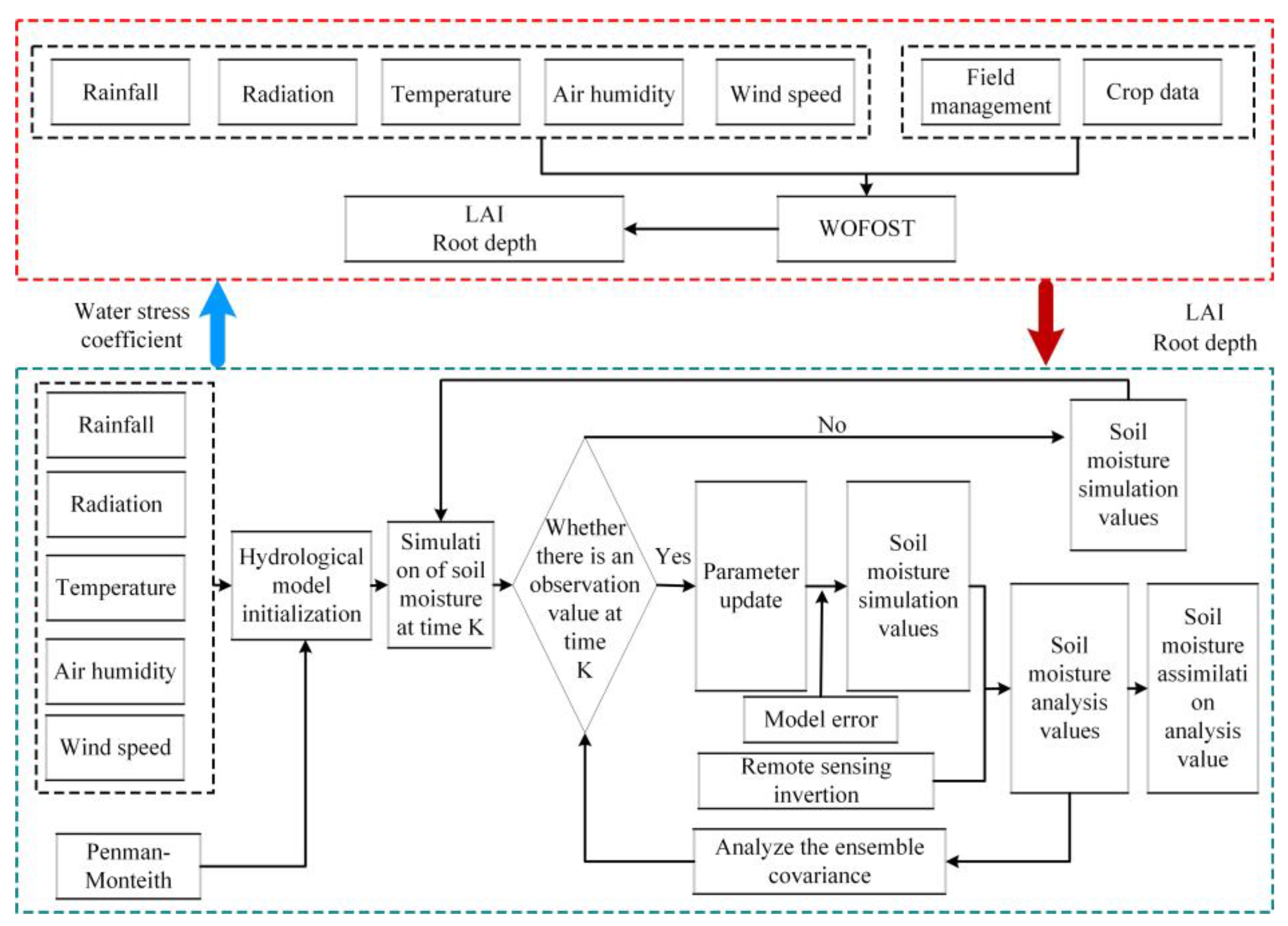
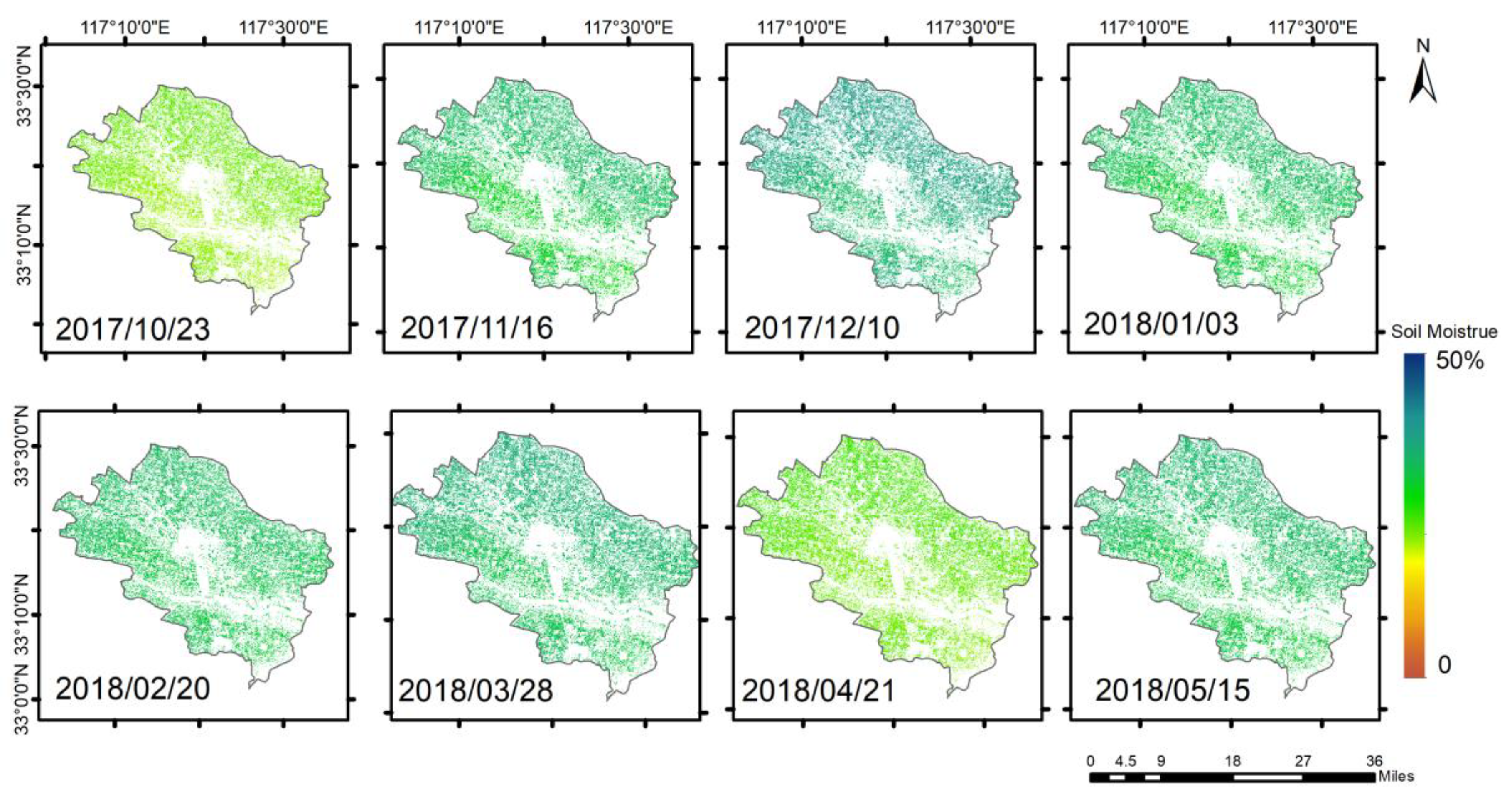
During the operation of the coupled model, when surface soil moisture data from remote sensing observation or inversion existed during the whole wheat growth cycle, assimilation analysis was performed with the surface soil moisture simulated by the coupled model. For the assimilation analysis of surface soil moisture, the surface soil moisture based on remote sensing observation data and water-cloud model inversion was constrained to the soil moisture data simulated by the coupled model throughout the reproductive period. Through the assimilation analysis of surface soil moisture in the coupled model, the accuracy of hydrological parameters simulated by the hydrological model is improved and transferred to the crop-growth model to obtain soil moisture based on the assimilation analysis. The framework for assimilation is shown in Figure 4.

The Ensemble Kalman Filter is a sequential data assimilation algorithm first proposed by Evensen in 1994 [38]. It uses a Gaussian-distributed state aggregate (let the number of sets be N) to represent the probability density function in a stochastic dynamic forecast, calculates the probability density function of the state aggregate at the next moment by forward integration and obtains the statistical properties (e.g., mean and covariance) at that moment. The Ensemble Kalman Filter consists of two steps: prediction and update. The data assimilation steps in this paper are as follows:

(1)

Initialize the background field. Given N Gaussian-distributed random variables $X_{i,}{}_0 (i=1,2,\dots ,N)=(X_1, X_2, X_3,\dots ,X_N)$, the state variables in this paper are the volumetric soil moisture content of each layer in the soil profile;

(2)

Calculate the forecast value $X_{i,k+1}^f$ for each random variable at moment $k+1$;

(3)

Calculate the Kalman gain matrix $K_{k+1}$ at moment $k+1$;

(4)

Calculate the analytical ensemble mean $\overline{X_{k+1}^a}$ and the analytical ensemble covariance $P_{k+1}^a$ for the state variables at moment $k+1$;

(5)

Go to the next moment and repeat iterative processes (2) to (5) until the end of assimilation.

Simulated results are compared with the measured results by the following four qualitative standards: (1) Average MRE, (2) Root-Mean-Square Error RMSE, (3) the determination coefficient, $r^2$, and (4) Nash–Sutcliffe Efficiency Factor (NSE):

$$MRE=\frac{1}{N}\sum _N^{i=1}\frac{\left(M_{sim,i}-M_{obs,i}\right)}{M_{obs,i}}\times 100\%$$

(21)

$$RMSE=\sqrt{\frac{1}{N}\sum _N^{i=1}{\left(M_{sim,i}{}_i-M_{obs,i}\right)}^2}$$

(22)

$$r^2=1-\frac{\sum {\left(M_{sim,i}-M_{obs,i}\right)}^2}{\sum {\left(M_{sim,i}-\overline{M_{sim}}\right)}^2\sum {\left(M_{obs,i}-\overline{M_{obs}}\right)}^2}$$

(23)

$$NSE=1-\frac{{\displaystyle \sum _{i=1}^n{\left(M_{obs,i}-M_{sim,i}\right)}^2}}{{\displaystyle \sum _{i=1}^n{\left(M_{obs,i}-\overline{M_{obs}}\right)}^2}}$$

(24)

where N is the number of observed values of soil moisture, $M_{obs,i}$ is the measured soil volumetric moisture content, $\overline{M_{obs}}$ is the mean value of measured soil volumetric moisture content, $\overline{M_{obs}}$ is the mean value of simulated soil volumetric moisture content and $M_{sim,i}$ is the simulated soil volumetric moisture content. The larger the NSE value, the closer the simulated result will be to the measured value.

3.6. Construction of Waterlogging Damage Identification Criterion

In Guzhen County, where winter wheat is usually sown in early October and harvested at the end of May, we chose the simulation results to analyze the risk of impregnation in Guzhen County from 11 October 2017 to 27 May 2018. Xu et al. proposes the standardized soil moisture index (SSMI) to detect droughts [39]. The SSMI was selected as an indicator for assessing waterlogging in this paper. In the process of standardizing the data, the probability distribution of soil moisture data needs to be determined. Therefore, the SSMI is constructed as follows:

$$\mathrm{SSMI}=\frac{SM-\overline{SM}}{\sigma }$$

(25)

where $SM$ is the soil moisture value at a certain time scale, $\overline{SM}$ is the mean soil moisture value at that time scale, and $\sigma$ is the standard deviation of soil moisture at that time scale. The soil moisture content of 0–10 cm soil layer is used as the main basis to discriminate the waterlogging, and then the waterlogging is considered to occur locally. The standardized moisture index for each growth period is obtained according to the daily scale of each growth period. The time of the wheat growth period referring to Yu et al. and combining with the local statistics of the research area [40], which is shown in

Table 3. Time of each growth period.

Growth Period	Sowing Stage	Pre-Winter Seedling Stage	Wintering Stage	Jointing Stage	Booting Stage	Heading and Filling the Stage
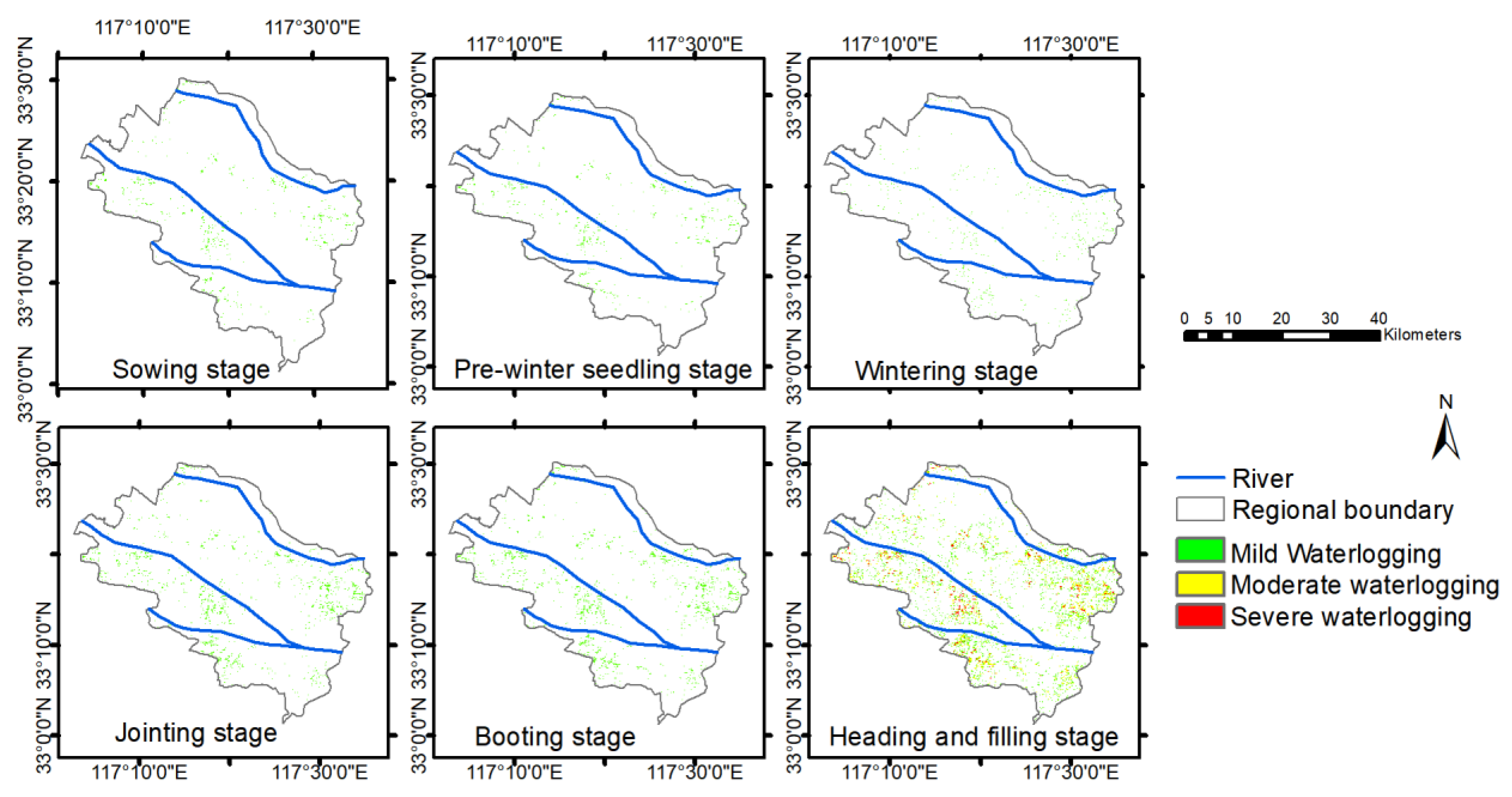
time	October	November–December	January–February	March	Early April–mid-April	Late April–mid-May

. The separation point between waterlogging and non-waterlogging is 1.5σ of the data. The soil moisture data are tested to be normally distributed, and the calculated SSMI obeys the standard normal distribution (μ = 0; σ = 1). The average value of soil moisture in each growth period is counted, and when it is greater than the value, the waterlogging rate distribution in Guzhen County is monitored as a risk area for waterlogging. Based on the above waterlogging damage criteria, the formula for calculating the waterlogging damage ratio R is as follows:

$$\mathrm{R}=\mathrm{n}/\mathrm{N}$$

(26)

where $\mathrm{n}$ is the sum of days of waterlogging and $\mathrm{N}$ is the total number of days in each growth period. The study area is divided into four waterlogging levels, which refers to Zhang et al. [13]: no waterlogging area, mild waterlogging area (R greater than 0.1 and less than 0.3), moderate waterlogging area (R greater than 0.3 and less than 0.6) and severe waterlogging area (R greater than 0.6).

4. Results

4.1. Parameter Calibration

Just like running a hydrological or vegetation model alone, running the coupled model requires the calibration of crop growth and development parameters related to crop phenology development, CO₂ assimilation, crop respiration and dry matter allocation, as well as soil hydraulic parameters. The WOFOST model comes with several crop-specific parameter files, but in practice, it is necessary to create new crop parameter files or adapt existing crop parameter files to the genetic characteristics of the crops grown. In this study, the crop growth parameters are determined by taking into account the growing environment (radiation, temperature, etc.) and the crop growth cycle, and are adjusted using the extended Fourier amplitude sensitivity test (EFAST) optimization program that comes with the WOFOST model. The calibrated values and units of the crop parameters to be adjusted are given in

Table 4. Calibration results of parameters.

Parameters	Definition	Calibrated Values	Units
TSUM1	The cumulative temperature from emergence to flowering	1000	${ }^{\circ }\mathrm{C}\cdot \mathrm{d}$
TSUM2	The cumulative temperature from flowering to maturity	1050	${ }^{\circ }\mathrm{C}\cdot \mathrm{d}$
TDWI	Initial dry matter weight	100
LAIEM	Leaf area index at seedling emergence	0.044	ha$\cdot {\mathrm{ha}}^{-2}$
RGRLAI	Maximum leaf area index relative growth rate	0.029	${\mathrm{ha}}^2\cdot {\mathrm{h}}^{-2}\cdot {\mathrm{d}}^{-1}$
TBASE	Lower temperature limit for leaf survival	10	${ }^{\circ }\mathrm{C}$
CVL	The efficiency of assimilating conversion to leaves	0.69	$\mathrm{kg}\cdot {\mathrm{kg}}^{-1}$
FLTB 0.0	Percentage of the surface area of the dry matter assigned to the foliage (DVS = 0)	0.62	$\mathrm{kg}\cdot {\mathrm{kg}}^{-1}$
FLTB 0.33	Percentage of the surface area of the dry matter assigned to the foliage (DVS = 0.33)	0.60	$\mathrm{kg}\cdot {\mathrm{kg}}^{-1}$
FLTB 0.88	Percentage of the surface area of the dry matter assigned to the foliage (DVS $=0.88$)	0.50	$\mathrm{kg}\cdot {\mathrm{kg}}^{-1}$
FLTB 0.95	Percentage of the surface area of the dry matter assigned to the foliage (DVS $=0.95$)	0.30	$\mathrm{kg}\cdot {\mathrm{kg}}^{-1}$
FLTB 1.10	Percentage of the surface area of the dry matter assigned to the foliage (DVS $=1.10$)	0.25	$\mathrm{kg}\cdot {\mathrm{kg}}^{-1}$
FLTB 1.20	Percentage of the surface area of the dry matter assigned to the foliage (DVS $=1.20)$	0.03	$\mathrm{kg}\cdot {\mathrm{kg}}^{-1}$
SLATB 0.00	Specific leaf area (DVS $=0.00)$	0.0026	$\mathrm{ha}\cdot {\mathrm{kg}}^{-1}$
SLATB 0.78	Specific leaf area (DVS = 0.78)	0.0012	$\mathrm{ha}\cdot {\mathrm{kg}}^1$
SLATB 2.00	Specific leaf area (DVS = 2.00)	0.0012	$\mathrm{ha}\cdot {\mathrm{kg}}^{-1}$
AMAXTB 0.00	Maximum assimilation rate of ${\mathrm{CO}}_2$ (DVS $=0.00)$	55	${ \mathrm{kg}}^2\cdot {\mathrm{ha}}^{-2}\cdot {\mathrm{h}}^{-1}$
AMAXTB 1.25	Maximum assimilation rate of ${\mathrm{CO}}_2$ (DVS =1.25)	50	${ \mathrm{kg}}^2\cdot {\mathrm{ha}}^{-2}\cdot {\mathrm{h}}^{-1}$
AMAXTB 1.50	Maximum assimilation rate of ${\mathrm{CO}}_2 \left(\mathrm{DVS}=1.50\right)$	40	${ \mathrm{kg}}^2\cdot {\mathrm{ha}}^{-2}\cdot {\mathrm{h}}^{-1}$
AMAXTB 1.75	Maximum assimilation rate of ${\mathrm{CO}}_2$ (DVS = 1.75)	35	${ \mathrm{kg}}^2\cdot {\mathrm{ha}}^{-2}\cdot {\mathrm{h}}^{-1}$

. Default values are used for the remaining parameters.

For the HYDRUS-ID model in the coupled model, the soil water movement in the vertical direction and the equilibrium module are influenced by the soil water potential variation and hydraulic conductivity parameters. The parameters to be determined include residual water content (${\theta }_r,{\mathrm{cm}}^3\cdot {\mathrm{cm}}^{-3}$), saturated water content (${\theta }_s,{\mathrm{cm}}^3\cdot {\mathrm{cm}}^{-3}$), saturated hydraulic conductivity (${\mathrm{K}}_{\mathrm{s}},\mathrm{cm}\cdot {\mathrm{d}}^{-1}$), inlet suction parameter ($\alpha ,{\mathrm{cm}}^{-3}$), pore size distribution parameter (n, dimensionless), etc. The parameters used in this paper are referenced in Zhou et al. [14].

4.2. Coupled Model Simulation Results

Based on the meteorological data observed at the stations, the coupled model is driven and the hydrological parameters interact with the crop parameters day-by-day obtain continuous (day-by-day) soil moisture data for the growing season. Soil moisture is simulated from 11 October 2017 to 27 May 2018, and the simulated values of soil volumetric moisture content are compared with the observed values of soil volumetric moisture content. When comparing the observed soil moisture data with the rainfall data, it shows that soil moisture is influenced by rainfall, with more pronounced fluctuations occurring around the time of the rainfall. The time series of the simulated and observed values are shown in Figure 3. The trends of the simulated and observed values of soil volumetric moisture content at the three monitoring sites are generally consistent, especially in October, November and December. From Figure 5, it can be seen that the simulated results of soil volumetric moisture content are relatively close to the measured values, with the Nash–Sutcliffe efficiency (NSE) of 0.528, 0.575 and 0.541. The variation tendency of the simulated water content was similar to that of measurement, but there was still some error in simulation and measurement. Qualitative standard comparisons of simulation results with measurements indicate that HYDRUS-1D and WOFOST have good accuracy in predicting soil moisture, which is shown in

Table 5. Qualitative standards for the simulated results compared with the measured results.

Site	r2	RMRE	MRE (%)	NSE
Site1	0.82	0.021	11.67	0.528
Site2	0.85	0.023	12.37	0.575
Site3	0.81	0.020	9.916	0.541

. Figure 5 also illustrates temperature and precipitation at the measurement sites. Soil moisture is related to a variety of factors including evapotranspiration, precipitation and drainage. Temperatures gradually increased between March and May, which increased the evapotranspiration effect of soil moisture. Because of the addition of measuring equipment and the high terrain at these three measurement sites, Figiure 5 shows a lack of consistency between soil moisture data in response to rainfall events in some time.

4.3. Soil Moisture Inversion and Assimilation

The Ensemble Kalman Filter algorithm is used as the assimilation algorithm in this study. In Figure 6, the NSE coefficients of the locations calculated from the measured and simulated values are relatively high. It can be seen from Figure 6 that the simulated results for soil volumetric moisture content are close to the measured values with NSEs of 0.752, 0.731 and 0.692. There is a significant improvement compared with Figure 5. Qualitative standards shown in

Table 6. Qualitative standards for the simulated results after assimilation compared with the measured results.

Site	r2	RMRE	MRE (%)	NSE
Site1	0.91	0.020	10.29	0.752
Site2	0.93	0.018	9.35	0.731
Site3	0.89	0.013	6.92	0.692

also indicate that the decline in RMSE and MRE, the rise in r² and the EnKF have some effect on the accuracy of the model.

4.4. Regional Soil Moisture Distribution

The distribution of soil moisture content after assimilation in Guzhen County from October 2017 to May 2018 is shown in Figure 7. The relative soil moisture content in Guzhen County was relatively low in October and November 2017, because the winter precipitation was low during that time. With the onset of spring, the soil moisture content in Guzhen County decreases to lower levels. Soil moisture content rises in Guzhen County during the summer months of February through May, which is consistent with Guzhen County’s climate characterized by abundant summer rains. As precipitation is higher in the south than in the north of Guzhen County most of the time, and as there are more low-lying areas in the south with low terrain and proximity to the Xi’an River, the moisture content is mostly higher in the south than in the north.

4.5. Distribution of Waterlogging

The waterlogging damage disaster risk map of Guzhen County is shown in Figure 8. The distribution of waterlogging levels shows that most of the waterlogging areas are mild waterlogging, which is interspersed with a small amount of moderate and severe damage. Most of the damage occurred during the plucking, gestation and filling stages of winter wheat, which is associated with the high precipitation from March to May. The waterlogging areas are generally distributed relatively evenly, with more severe damage in the low-lying areas. The statistical description of the damage risk in each subdistrict is as follows: no waterlogging area accounts for 50.7% of the winter wheat field area in Guzhen County, mainly in the higher terrain. Mild waterlogging area accounts for 20.7% of the winter wheat field area in Guzhen County. Moderate waterlogging area accounts for 16.5% of the winter wheat field in Guzhen County. The severe waterlogging area accountsfor 12.1% of the winter wheat field area in Guzhen County.

4.6. Evaluation of Waterlogging Damage

Winter wheat yield reduction rate data for 11 towns in Guzhen County from 2017 to 2018 are obtained from the Guzhen County statistical yearbook information, as shown in Figure 9. Waterlogging areas are mainly concentrated in areas with relatively low terrain and water catchment areas. The yield reduction rate is low in most towns and slightly higher in towns with lower terrain and near rivers.

The proportion of farmland area affected by inundation and the rate of yield reduction in each township are shown in

Table 7. The percentage of area affected by waterlogging in each township and the rate of yield reduction.

Town	Waterlogging Area Percentage %	Yield Reduction Rate %
Chengguan	16.98	−4.34
Wangzhuang	25.72	−4.75
Xinmaqiao	34.54	−5.35
Liancheng	35.14	−6.37
Liuji	49.19	−10.13
Renqiao	10.56	−3.87
Hugou	45.67	−7.48
Haocheng	14.77	−4.13
Shihu	23.16	−4.52
Yangmiao	43.79	−6.62
Zhongxin	16.98	−4.34

. Due to the high rainfall in 2018, there are no major changes in agricultural technology, and the townships has experienced different degrees of yield reduction.

The correlation between the percentage of the waterlogging area and the yield reduction rate for each township in 2017–2018 is calculated and shown in Figure 10. The results show that the percentage of waterlogging area in each township is highly significantly and positively correlated with the yield reduction rate of winter wheat (R = 0.78). In general, there is good agreement between the statistical data-based yield reduction rate of winter wheat and the percentage of affected farmland assessed based on the waterlogging identification criterion. However, the rate of yield reduction in some towns does not exactly increase with the area affected. The main reason is that grain yield reduction may be caused by various reasons, e.g., in the category of agro-meteorological hazards, it may be caused by high winds and hail in addition to waterlogging.

5. Discussion

5.1. Factors Influencing Model Results

According to Liu and Gupta [41], the sources of uncertainty in modeling are the model structure, parameters and data. The data used as inputs or initial conditions to the model may have measurement errors due to the nature of the instrumentation used or representation errors due to spatial or temporal incompatibilities. Uncertainty can also arise due to errors in the estimation of parameters used in the model. Wagener et al. argue that parameter uncertainty can be minimized by using more output variables, reducing the complexity of the model, and increasing the information available to determine the model parameters [42]. Wagener and Gupta relate uncertainty in the model structure to a real-world process that is linked to simplification [43].

Errors in the individual models described above can propagate into the coupled model, thereby compounding the level of uncertainty. The nature of the coupling can also induce another type of uncertainty in the coupled model. According to Antle et al., the coupled model can lead to additional conceptualization and computational problems, thus increasing the level of uncertainty [44]. The experimental area as a whole is not very high in elevation, but there are parts of the area where the terrain is undulating. Rainfall is therefore discharged by gravity, so that whenever larger rainfall is generated, the surface water content varies considerably and persists for a period of time, easily generating internal flooding in local areas. The climate of Guzhen County is a warm temperate semi-humid monsoon climate with cold, dry winters and warm, hot, rainy summers. When the rainfall is high, it tends to show a peak on the curve, the simulated value will have some error with the real value, and the error will last for a long time. This indicates that the simulation accuracy of the model is reduced under the influence of extreme weather with high precipitation.

5.2. Assimilation System Improvements

The data assimilation method combines the inverted data from remote sensing inversion and the simulated data from the HYDRUS-1D and WOFOST coupled model to obtain more accurate assimilated data. Firstly, the state variable assimilated in this study is a single variable SM, but the parameters of the HYDRUS-1D and WOFOST coupled model may change over time during the experiment, so the data assimilation scheme with dual or multiple state variables may have more potential for the study. Secondly, there is room for improvement in the construction of the Ensemble Kalman Filter assimilation algorithm used in this study. This study used experimental data from 11 October 2017 to 27 May 2018 for data assimilation tests. The amount of data is still small and the time series is short, which cannot provide a better prediction of soil moisture. The assimilation accuracy can be further improved in future studies by using multiple years of data for assimilation and selecting some data as assimilation data sets and some data as calibration data sets.

5.3. Analysis of Factors Influencing Waterlogging Damage

The factors affecting winter wheat waterlogging damage include atmospheric precipitation, soil physical properties, groundwater level, topography, drainage and irrigation conditions, tillage system and crop resistance to stains. The most obvious influencing factor is the topography, and the average elevation of different affected areas is counted (as shown in

Table 8. Relationship between DEM and spatial distribution of surface relative humidity in dryland soils.

Waterlogging Level	Area Ratio	DEM Average/m	DEM Variance
No waterlogging	50.7%	15.18	5.57
Mild waterlogging	20.7%	1.47	2.4
Moderate waterlogging	16.5%	−2.12	2.24
Severe waterlogging	12.1%	−10.32	1.94

), it can be seen that the average elevations of the areas in different waterlogging levels have obvious difference, and the elevation of the severe waterlogging area is the lowest, followed by the moderate, mild and no waterlogging areas. However, waterlogging is the result of the comprehensive influence, the place with low topography is not a heavily affected area if the river network is dense. Guzhen County is the most seriously affected in heading and filling the stage, as shown in Figure 6. In the northern area of Guzhen County, the terrain is high and the topography is not very undulating, so it is not affected by the impregnation. In the central and southern regions, the topography is more undulating and the low-lying areas are prone to rainwater pooling and are more severely affected. However, some areas are only lightly impregnated despite the low terrain. This is due to the proximity to rivers, where the impregnated water drains faster, resulting in a lower degree of waterlogging.

5.4. Limitations and Applicability

Waterlogging damage monitoring needs to consider the continuity of the features present in the soil of the affected farmland. To address the temporal discontinuity problem in satellite-borne synthetic aperture radar (SAR) inversion of soil moisture, this paper synthesizes the advantages of the two models by coupling the crop growth model with the hydrological model to achieve the goal of accurate soil moisture simulation. The assimilation method of remote sensing inversion data effectively reduces the uncertainty of the original coupled model and provides an effective method for obtaining the spatial and temporal continuous distribution information of soil moisture. However, the inconsistent temporal frequency and spatial resolution of multi-source data, as well as the data acquisition mechanism of each sensor, may lead to bias among the data. In future research, how to minimize the error of the final results by testing and validating the multi-source remote sensing data and how to equalize the error between each data source should be addressed. In addition, this paper used the duration of soil moisture as the eigenvalue to measure the degree of wheat impregnation, which is insufficient to quantify the differences in wheat impregnation tolerance during different fertility periods. In order to construct a comprehensive damage index to reflect the degree of wheat damage and accurately assess the risk of damage, it is necessary to further quantitatively characterize the degree of wheat damage, and at the same time, consider the effect of soil hypoxia on the root system and the differences in the tolerance of wheat during different growth periods, and then substitute the results of soil surface moisture for the risk assessment of damage.

6. Conclusions

This study aims to estimate the loss of winter wheat in waterlogging with higher accuracy and resolution. The remote sensing inversion results are assimilated with the HYDRUS-1D and WOFOST coupled model using an Ensemble Kalman Filter algorithm to obtain more accurate soil moisture. The simulated values of HYDRUS-1D and WOFOST coupled model differs significantly from the measured values, but the spatial extent shows an actual trend. During the assimilation process, remote sensing data plays an effective role in correcting the simulation results. The use of remotely sensed data as a reference has a special impact on the internal prediction mechanism of the particle filter when the simulated results differ significantly from the measured data in terms of trends and numerical variations. Thus, the obtained simulation values integrate not only the accuracy of remote sensing inversions but also the physical mechanisms of model simulations. Finally, an integrated waterlogging hazard identification criterion is established. The identification criterion estimates a significant correlation between the waterlogged area and the yield reduction rate of winter wheat, and the waterlogged area can indicate the yield reduction of winter wheat caused by waterlogging of farmland. The results indicate that the regional waterlogging evaluation system supports large-scale winter wheat waterlogging monitoring and has the potential for application. Compared with the spatial distribution zoning using a single factor of climatic elements, it integrates consideration of the effects of meteorological conditions, topography, crop type, soil type and hydrological elements, thus improving the estimation accuracy.