Article

Fast Adaptive Beamforming for Weather Observations with Convolutional Neural Networks

1
Advanced Radar Research Center, University of Oklahoma, Norman, OK 73019, USA
2
School of Electrical and Computer Engineering, University of Oklahoma, Norman, OK 73019, USA
3
School of Meteorology, University of Oklahoma, Norman, OK 73019, USA
*
Author to whom correspondence should be addressed.
Remote Sens. 2023, 15(17), 4129; https://doi.org/10.3390/rs15174129
Submission received: 14 July 2023 / Revised: 14 August 2023 / Accepted: 16 August 2023 / Published: 23 August 2023

Abstract

:
Polarimetric phased array radar (PAR) can achieve high temporal resolutions for improved meteorological observations with digital beamforming (DBF). The Fourier method performs DBF deterministically, and produces antenna radiation patterns with fixed sidelobe levels and angular resolution by pre-computing the beamforming weights based on the geometry of receivers. In contrast, the Capon method performs DBF adaptively in response to the changing environment by computing the beamforming weights from the received signals at multiple channels. However, it becomes computationally expensive as the number of receivers grows. This paper presents computationally efficient adaptive beamforming with an application of convolutional neural networks, named ABCNN. ABCNN is trained with the phase and amplitude of complex-valued time-series IQ signals and the Capon beamforming weights as input and output. ABCNN is tested and evaluated using simulated time-series data from both point targets and weather scatterers for a planar of fully digital PAR architecture. The preliminary results show that ABCNN lowers computation time by a factor of three, compared to the Capon method, for a phased array antenna with 1024 elements, while mitigating the contamination from sidelobes by placing nulls at the location of the clutter. Furthermore, ABCNN produces antenna patterns similar to those from the Capon method, which shows that it has successfully learned the data.

1. Introduction

The phased array radar (PAR) is composed of many subsystems and components, one of which is the antenna. It enables the use of electronic steering, beamforming, and other capabilities that are different from conventional reflector-antenna radars [1,2]. Controlling the amplitude and phase of antenna elements can allow the radar to steer a beam to the desired direction electronically within its visible region. Furthermore, digital PAR offers maximum flexibility in scanning strategies. It can perform different scanning patterns, including those transmitting “pencil” beams, spoiled beams, and/or multiple beams in different directions [3]. Digital beamforming (DBF) is a unique capability of PAR, which is accomplished by transmitting a spoiled beam and simultaneously receiving multiple narrow (i.e., pencil) beams within the transmit envelope. Therefore, DBF can sample a large sector of the atmosphere with an improved temporal resolution by reducing the need for mechanical rotation [4]. The “Horus” radar is a fully digital, S-band, polarimetric PAR that was developed by the Advanced Radar Research Center (ARRC) at the University of Oklahoma, and funded by the National Oceanic and Atmospheric Administration (NOAA) [5]. It is a rotating PAR (RPAR) that can steer the beam electronically in the elevation and/or azimuth and rotate mechanically in the azimuth. Its antenna is composed of up to 1600 (40 × 40) fully digital polarimetric elements that transmit and receive independent electromagnetic waves. Horus has the most promising PAR architecture to meet the requirements needed for multi-mission radars, in terms of both weather and aircraft surveillance [3,6]. It should be mentioned that due to cost constraints, the planned array size for Horus is 1024 (32 × 32), which will be assumed in the remainder of this paper.
The DBF method is used to produce and simultaneously receive beams in the angular direction of interest by multiplying the beamforming weights and the received signals. The beamforming weights can be calculated in either a data-independent or data-dependent way. The Fourier method is data-independent, and it can be used to pre-determine the beamforming weights based on the geometry of the digital sub-arrays or antenna elements. It provides a way to calculate the needed phase shift between receivers (i.e., elements) to synthesize the receiving beam in the desired direction. Therefore, the Fourier method produces beam patterns with the determined shape and sidelobe levels, which result in a fixed angular resolution. It may lead to high sidelobe levels in undesired directions, where clutter or interference may be located, which can significantly contaminate the received signals. In contrast, the Capon method is data-dependent and calculates the beamforming weights based on the received signals. It can place nulls adaptively in the directions with undesired high-power returns caused by the ground clutter or interference, thus it minimizes the total power [7,8]. This results in improved data quality compared to the Fourier method. However, the Capon method becomes computationally expensive as the size of the antenna grows, limiting the real-time implementation.
Optimized DBF methods have been studied widely. The particle swarm optimization algorithm performs adaptive DBF by controlling the excitation of each array element, in order to focus the signal in the desired direction and minimize power by imposing nulls at the undesired direction where inference is located for the uniform circular arrays [9]. The evolved particle swarm optimization with the firefly algorithm for a non-uniformly spaced linear antenna array is introduced in [10]. This algorithm optimizes the spacing between the array elements through the firefly algorithm to create a predefined arbitrary radiation pattern that satisfies the requirements of the sidelobe levels, beamwidth, and null, while keeping the constant excitation amplitude for the elements. The genetic algorithm has also been studied for adaptive wide null steering for linear and circular arrays in [11]. The proposed genetic algorithm suppresses the sidelobe levels with multiple deep nulls while maintaining the original sidelobe level. However, wider widths of the null cause the higher sidelobe levels as a trade-off. Furthermore, this algorithm presents a limitation of direct real-time processing.
Artificial intelligence (AI) has been widely applied in various fields because of its flexibility and adaptability. It has established a new approach to tackle high-complexity, nonlinear problems. One of the AI subfields, known as machine learning (ML), is an efficient data analysis tool, and is capable of identifying patterns in complex data sets. For example, ML has been used for storm-mode classifications, classification of precipitation types, tornado predictions, and hail predictions in radar meteorology applications [12]. A comprehensive review of ML in radar meteorology is provided in [13]. Deep learning (DL), a subset of ML, is a technique that makes use of neural networks with multiple layers to create complex mappings that connect inputs to outputs. Compared to traditional ML, DL is inspired by the human brain to learn of the complex relationships between data [14].
The application of DL for fast adaptive DBF in many different domains has been widely studied recently (see Table 1). A neural network with dense layers (i.e., a fully connected layer), named ABLE, was designed to perform adaptive beamforming for biomedical imaging in [15]. ABLE is trained to reproduce the downstream system output, not directly reproduce the values of beamforming weights, to lower the computational complexity of the neural network. Another format of DL is the least-mean-square (LSM) algorithm, which has been studied for fast adaptive beamforming with a lower complexity of neural networks in [16]. Furthermore, DL has been applied to perform matrix inversion in order to fasten the adaptive DBF process with weather radars in [17]. Their work specifically tackles the issue of matrix inversion, which is the primary cause of the computational burden of adaptive DBF methods. They propose a radial-basis-function neural network (RBFNN) that is trained to take the covariance matrix of received signals as input, and produces beamforming weights as an output to perform real-time adaptive DBF. Even though RBFNN was designed to improve temporal resolution while maintaining the quality of data, the preliminary results have shown limitations. RBFNN can only process real-valued data; therefore, they ingested complex-valued data into real and imaginary parts. However, this results in an efficiency loss in the neural network design, which required doubled length and, more importantly, failure to preserve phase information. The loss of phase information is critical for neural networks to learn the relationship between time-series signals and beamforming weights. Furthermore, RBFNN is not designed to emulate the Capon beamforming weights. To preserve phase information of complex-valued data, a new design of neural network was explored in [18]. They propose a Deep Learning Adaptive digital Beamforming (DLAF), which was composed of layers that can ingest, process, and produce complex values with a specific library built on the TensorFlow platform, called the Complex-Value Neural Network (CVNN) [19], using the Python programming language. DLAF is designed with dense layers that connect nodes of the previous layer to nodes of the current layer. Dense layers can be a good choice for non-spatial data such as time-series signals. Because they fully connect neurons between layers and operate on a per-pixel basis, which can minimize loss while maximizing the learning process of complex data. DLAF was trained to take complex values of time-series IQ signals as input and produce complex values of the Capon beamforming weights as output. DLAF has successively reduced the computational time of adaptive DBF by eliminating the step of calculating the inversion of the covariance matrix. Even though DLAF was able to preserve the phase information of the data, it has a critical limitation in its architecture. Since CVNN is a personal library, it does not support many layers, which limits the flexibility and efficiency of the network design and training. Furthermore, the use of dense layers for the regression task can lead to learning saturation issues and high complexity of the neural network.
The motivation of this work is to minimize the computation burden of the adaptive beamforming method to enable real-time processing while improving the quality of weather observations by mitigating contamination caused by sidelobes. Therefore, an Adaptive digital Beamforming with CNN (ABCNN) is built to perform adaptive DBF with computational efficiency and training flexibility. ABCNN is built on TensorFlow, the Python platform, with a library called Keras [20]. Keras is one of the most widely used libraries for ML users, because of its flexibility in designing networks. It offers many different built-in and open-sourced layers, including activation, convolution, and dense [21]. However, Keras does not support complex values in the network at this moment. Therefore, the casting of complex values into real values is required. To preserve the phase information in the time-series signals and beamforming weights, complex values of these data are divided into phase and amplitude. Then, ABCNN is trained with the phase and amplitude information independently and in parallel. CNN is well-known for tasks with images or data that contain strong spatial information, as it learns data with convolution filters. Therefore, CNN was used to design ABCNN to learn the training data, which are time-series signals and beamforming weights at each receiver. The proposed method has several advantages over previous DL-based adaptive DBF methods: (1) the neural network takes time-series signals and produce directly the adaptive beamforming weights; (2) it preserves the phase information of data; and (3) it trains faster with fewer training samples (specifically compare to DLAF). Preliminary results of ABCNN show improved data quality compared to that produced using the Fourier method by emulating the adaptive DBF skill of the Capon method. More importantly, it has successfully reduced the computation time compared to the Capon method. It should be emphasized that the main contribution of this work is to mitigate the computational burden of the Capon method and permit real-time implementation for weather observations. The higher quality performance, better efficiency, and lower complexity of neural networks can be studied further in the future.
This paper is organized as follows. The background and mathematical derivations for deterministic and adaptive DBF methods are described in Section 2.1. A simulation scheme for digital PAR that uses pre-existing data from conventional reflector-antenna radars is developed in Section 2.2. Then, ABCNN is presented, including the design of the neural network, training data, and training strategy, in Section 2.3. Analyses of the preliminary results of ABCNN tested on simulated weather cases with clutter are presented in Section 3. The limitation of the current algorithm is discussed in Section 4. Finally, this work is concluded, and future works are discussed in Section 5.

2. Method

2.1. Background on Digital Beamforming Methods

Radar imaging refers to the capability of scanning a large sector of the atmosphere by DBF, which transmits a spoiled beam and forms multiple narrow receive beams spontaneously within the transmit envelope [2]. By doing this, PAR can reduce the scan time compared to the use of conventional pencil beams. Therefore, PAR with DBF can offer a better understanding of the atmosphere through a high temporal resolution [22,23]. This technique could be useful, especially for severe weather observations, such as tornadic storms, hail storms, and hurricanes, which evolve fast and require high temporal resolution observations [24].
DBF can estimate power in the direction of the wavenumber, which is defined as k = ( 2 π / λ ) [ sin θ sin ϕ sin θ cos ϕ cos θ ] , where θ and ϕ are the elevation and azimuth angles. The estimated power is defined as the equation follows [7],
P ( k ) = w H R w ,
where w is the beamforming weight for the receiver (N), H indicates the Hermitian operator, and R is the autocovariance matrix of received signals at N receivers. w is an N × 1 vector and R is an N × N matrix. The beamforming weights can be calculated in either a deterministic or adaptive way. The Fourier method is a deterministic DBF method that pre-computes beamforming weights based on the geometry of the antenna elements. Since the Fourier method is data-independent, it synthesizes receive beams with fixed sidelobe patterns and fixed angular resolution. However, this could be undesired when there is clutter or interference located inside the sidelobes, because clutter or interference will cause high power returns from undesirable directions with the fixed beam pattern and lower the quality of observations. In contrast, the Capon method, also known as the minimum variance distortionless response (MVDR), is an adaptive DBF method that computes the beamforming weights with received signals at each receiver. The Capon method can synthesize receive beams that can automatically adjust the antenna pattern and suppress high-power returns from undesired directions by placing nulls in the undesired directions. Therefore, it can mitigate the contamination from the sidelobes and minimize the total power of synthesized beams.

2.1.1. Deterministic Digital Beamforming

The Fourier method is implemented as a weighted sum of the element signals. It is used to compute beamforming weights by calculating the needed phase shift between antenna elements to electronically steer the beam in the desired direction k, as follows:
w f = [ e j k · D 1 e j k · D 2 e j k · D N ] T ,
where D i represents the position vector of the i th receiver, i = 1 , 2 , , N . Note that the Fourier beamforming weights result in the conventional steering vector [25].

2.1.2. Adaptive Digital Beamforming

The Capon method is a high-resolution estimation method that has shown robustness and the potential to reduce effects from interference [26]. This method was first implemented for atmospheric radar applications in [7]. It is a data-dependent technique that adaptively calculates the beamforming weights from the returned signals to improve the quality of data. It attempts to lower the sidelobe levels in directions with high power returns and minimize the power in all directions except the desired scan direction k [7,8]. This minimization problem is described mathematically as follows:
min w P ( k ) subject to e H w = 1 .
To solve this problem, standard Lagrange methods [27] were applied to the general form of power given Equation (1), as follows,
L ( w , γ ) = w H R w + γ ( e H w 1 ) ,
where γ is the Lagrange multiplier shown below [7],
γ = 2 e H R 1 e .
Finally, the Capon beamforming weights are computed as follows [4],
w c = R 1 e e H R 1 e ,
where e = w f is the steering vector, and R 1 is the inverse of the autocovariance matrix with a size of N × N .

2.1.3. Computational Complexity

The Fourier method involves only matrix multiplication, namely k · D , where k and D have a size of 1 × 3 and 3 × 1 , and each term represents beam steering direction and the geometry of receivers in the Cartesian coordinate system. This multiplication is repeated for every receiver (N). The complexity order of matrix multiplication of a n × m matrix and a m × p matrix, which produces a n × p matrix, will be O ( n m p ) [28]. Therefore, the complexity order of the Fourier method is O ( 3 N ) , which increases linearly with the number of receivers N. The Capon method involves the matrix inversion to calculate R 1 . The complexity order of the matrix inversion obtained by Gauss–Jordan elimination with a n × n matrix will be O ( n 3 ) [28]. Therefore, the complexity order of the Capon method will be O ( N 3 ) , which increases exponentially with N. Figure 1 shows the order of complexity in the logarithm scale as a function of the number of receivers for each DBF method. Specifically, at the size of Horus (1024), the complexity order of the Capon method and the Fourier method are 9.03 and 3.487 in the logarithm scale.

2.2. Simulation of Digital Array

Due to the lack of fully digital PAR data for weather cases, all the data used for training and testing ABCNN have been simulated based on the Next-Generation Radar (NEXRAD). It also gives the flexibility to add clutter targets on simulated weather signals, in order to evaluate the performance of clutter mitigation with DBF. The first step is to produce realistic time-series IQ signals from the pre-existing moment data obtained by NEXRAD. The second step is to expand the simulation of the reflector-antenna radar into the digital PAR with multiple receivers. This can be obtained by adding the required phase shifts between each receiver to simulated time-series IQ signals. Then, the signal from the spoiled beam is generated by superposition summation of simulated time-series IQ signals for DBF use. Details of each simulation step are explained next.
The simulation of weather-like time-series IQ signals, V j ( t ) , using pre-existing meteorological variables, has been previously developed [29,30]. Note that j = 1 , 2 , . . . , J and J represents the total number of time-series IQ signal realization from NEXRAD (i.e., the total number of simulated range gates). In this paper, archived NEXRAD data are read and processed by Python ARM Radar Toolkit (Py-ART), which is an open-source library for working with weather radar data [31]. Due to intrinsic radar characteristics and signal processing, it requires data conditioning for overlaid echoes in Doppler variables (labeled −888) and censored data (labeled −999) prior to the simulation. The overlaid echoes in Doppler variables are mitigated with a built-in function for de-aliasing velocity in Py-Art. Then, censored data are filled in with simulated noise.
NEXRAD data are from a reflector-antenna radar with a single digital receiver per polarization. Therefore, expansion of the simulation to generate digital PAR signals with multiple receivers is required for evaluating DBF methods. The digital PAR simulation was implemented using the fully digital Horus specifications shown in Table 2. Horus has a 2D antenna with 32 × 32 receivers; however, only the azimuth dimension (32 receivers) is simulated here. This is because NEXRAD only scans continuously in azimuth, and has several gaps in elevation. Therefore, spoiled beams are simulated for 1D DBF in azimuth only.
The simulation of digital PAR is described in Equation (7). It calculates the phase shift needed for each receiver by measuring the range from the center of transmit antenna to the target at time t, r T ( t ) , and the range from the target to the i t h receiver at time t, r R i ( t ) . Then, it is added to the simulated signals from the previous step, V j ( t ) , with a synthesized transmit beam pattern, f θ 2 , and the simulated noise, n T ( t ) . The synthesized transmit pattern that was designed for Horus in [32] is used for the simulation in this paper. The simulated transmit (i.e., spoiled) beam has a 10 beamwidth. The added noise is zero mean Gaussian-distributed white noise, where the variance was extracted from the NEXRAD KTLX data. Finally, signals from spoiled beams, V q ( t ) , can be generated by applying the superposition method to desired number of simulated signals, depending on beamwidth.
V q ( t ) = j = 1 n t f θ 2 V j ( t ) exp j 2 π λ ( r T ( t ) + r R i ( t ) ) + n T ( t ) ,
where λ is the wavelength and n t is the number of simulated IQ signals summed together to form a single signal for the spoiled beam. Then, Equation (7) is repeated for every spoiled beam to cover the desired azimuth section, noted as V q (t), where q = 1 , 2 , . . . , Q . Therefore, the total number of Q signals for the spoiled beam is simulated. Furthermore, two types of clutter are simulated and added to the simulated weather data. Note that all clutter signals were added prior to noise addition and summation of IQ signals to have the realistic signal-to-noise ratio (SNR) and accurate location of clutter. First, four stationary point targets (SPT) with 30 dB SNR were artificially added at various locations, with and without significant weather returns. The locations of SPTs are listed in Table 3. Since stationary point targets are delayed, echoes of the transmitted signal and do not produce a Doppler shift, the IQ signals at the i t h receiver for a point target can be simulated using the following Equation [33],
V i ( t ) = A i exp j 2 π λ ( r T ( t ) + r r R i ( t ) ) .
The second type is wind turbine clutter (WTC), which is considered dynamic clutter. WTC has been challenging to mitigate, because it creates nonzero Doppler returns as its blades rotate. Therefore, using adaptive DBF on WTC can show a data quality improvement compared to deterministic DBF. A total of eight WTCs are simulated following [34], and located close to the tornado hook echo, as listed in Table 3. Figure 2 shows a plane-position indicator (PPI) scan of the simulated model power (in dB) from the NEXRAD data collected on 20 May 2013, with artificially added clutter targets indicated as red dots in the plot.
Finally, DBF has been performed within the simulated spoiled transmit beams. Although the angular resolution of Horus is approximately 4 , DBF has been performed with azimuth oversampling at 1 for a better representation of simulated data and to more clearly see the benefits of adaptive DBF. The rotating PAR is simulated by changing the position vector of receivers, D, as it transmits a spoiled beam to different sectors. Transmit beam patterns overlap 27 (sidelobe region) at each end, to mitigate the discontinuities that occur between each transmit beam.

2.3. Adaptive Beamforming with CNN

The proposed ABCNN is built to perform fast adaptive digital beamforming and improve the efficiency and quality of training. ABCNN is a feed-forward deep neural network built on a Python platform using the Keras library. Keras offers many different open-source layers and functions to optimize the flexibility and feasibility of designing neural networks for different purposes. To use the advantages of Keras, all the data should be a real value, since it does not support complex-valued data at the moment. Therefore, complex values of time-series signals and beamforming weights that are used for training and testing are transformed into a phasor form (i.e., amplitude and phase) to avoid the loss of phase information caused when separating complex values into real and imaginary parts. Preservation of phase information of the IQ time-series signals and beamforming weights is critical for the neural network to be properly trained. Therefore, the network learns the amplitude and phase information independently and in parallel with different activation functions to increase learning efficiency. The proposed network consists of a mix of convolution layers, batch normalization layers, activation layers, a flatten layer, a dense layer, and a reshape layer. An overview of ABCNN is shown in Figure 3. This network is designed to take time-series IQ signals as inputs and produce beamforming weights for each receiver (N) at specific angular directions ( ϕ ) as output. It should be emphasized once more that the main contribution of this work is to mitigate the computational burden of the adaptive DBF method with an application of AI, and further studies on the performance of neural networks can be performed in the future.

2.3.1. Architecture of the Neural Network

Time-series signals (input) and desired beamforming weights (output) at each receiver have spatial information, but it may be subtle compared to typical image data. Therefore, ABCNN was designed to extract the spatial information of these two data sets with convolution layers. The architecture of the proposed network is shown in Figure 3. As is shown in the figure, inputs are 2D data, ( N , M ) , where M represents radar samples (i.e., pulses) and outputs are 2D data, ( N , b ) , where b represents the number of the beamforming index. Note that the first dimension represents the vertical axis and the second dimension represents the horizontal axis of training data. More details about preparing data for the neural network will be discussed in Section 2.3.3. The network starts with an input layer (blue) and has three sets of convolution (pink), normalization (orange), and activation (purple) layers.
First, the network extracts the important spatial features from the input data with three convolution layers with 64 filters and a kernel size of ( 3 , 15 ). Kernel size can be flexible, but a longer kernel size in the second dimension is desired for better learning. This is because the convolution filters scan the data along the second dimension. The 64 convolution filters are used in this model to improve the quality of learning, but also to keep the efficiency of learning time. Then, the output of the convolution filters is normalized with batch normalization. The use of normalization functions inside the model can keep the consistency among the data during the training. Furthermore, excessive data loss and domination of data from certain locations (e.g., strong storm area) over other locations (e.g., mild storm area) can be prevented by performing normalization of data before the use of activation functions. Phase data ( π , π ) are normalized by dividing the data sets by π , and amplitude data are normalized by their overall maximum value. Next, the activation layer is applied to activate the neurons inside the data. The use of activation functions after each convolution layer can help the network to create complex mappings between nodes. The role of the activation layer is an important feature of neural network learning, and more details will be discussed in the following section. The extracted data from the set of convolution filters are flattened into 1D signals with a flatten layer (green). Then, the data go through a dense layer (yellow), where all the neurons are fully connected and the complex mapping between the data is created. Finally, the 1D data are reshaped back into 2D metrics to match the output data size. The reshape layer gives flexibility in the size of data, which allows different radar settings (i.e., different numbers of radar samples M, or different numbers of beamforming index b). The network calculates the bias between the outputs from the model and the truth data with the mean-square-error (MSE) loss function, which is one of the most common loss functions. The learning weights are updated over many epochs (i.e., iterations). The optimal goal of having many epochs over the training data is to minimize the bias between the prediction and the truth.

2.3.2. Activation Functions

Activation functions play an important role in the learning process, as they sort out complex data and create meaningful mappings between data in each layer. They transform the activation level of input neurons to output neurons [35]. Therefore, two different types of activation function are selected for phase and amplitude training, to optimize the accuracy and efficiency of the training. The Rectifier Linear Unit (ReLU) activation function, well known for image-related ML tasks which contain all positive valued data with non-linear changes, is used to train amplitude data. The function, g ReLU ( x ) with the input x, is defined as follows,
g ReLU ( x ) = max ( x , 0 ) .
It activates the input linearly if it is a positive value, and vanishes if it is a non-positive value. However, ReLUs do not work for phase training, since phase data contain negative values with non-linearity changes. Therefore, the Hyperbolic tangent (tanh) activation function is introduced to the network for the phase training. The tanh function, g tanh ( x ) with the input x, can be mathematically described as follows,
g tanh ( x ) = e x e x e x + e x .
It can ingest and produce both negative and positive values. Furthermore, it can handle non-linear changes, and has balanced saturation limits both on negative and positive sides. As long as the data are normalized properly, using the tanh activation function will avoid excessive data loss.

2.3.3. Training Data

This section will discuss how to prepare training and testing data for ABCNN. The data are shaped for the use of 2D convolution filters, which are applied across the horizontal direction. First, input data for this network is the time-series IQ signals, which have four dimensions, including the number of transmit beams, range gates, receivers (N), and number of time samples (M). The first and second dimensions of the time-series signals represent the realization of the signal at each pixel, and can be combined to represent the number of training samples (a). Therefore, the size of the input data is ( a , N , M ) , and the network learns each input with a size of ( N , M ). Note that the order of dimension is important for the neural network to learn the spatial relationship between the time-series signals at each receiver, as the convolution filter is applied horizontally. Second, output training data for this network is adaptive beamforming weights from the Capon method. It also has four dimensions, including the number of transmit beams, range gates, receivers (N), and beam index (b). The first and second dimensions, which represent the realization of beamforming weights at each pixel, are combined together, and represent the number of training samples (a). Then, the output training data have a size of ( a , N , b ) , and the network learns each output with a size of ( N , b ) .
A total of 561 simulated IQ realizations (17 transmit beams and 33 range gates) of the tornadic supercell storm case (20 May 2013 19:59:14 Z) and corresponding adaptive beamforming weights from the Capon method were used in the training. These data were trained with a total of 5000 epochs for 18 h. The input, weather IQ signals with Horus specifications, has a size of N = 32 and M = 64 . The output, the Capon beamforming weights, has a size of N = 32 and b = 6 .

2.3.4. Training Strategy

The proposed network was trained in batch mode. A batch is defined as a group of data x, B = x 1 , x 2 , . . . , x m , where m is the number of data inside a batch. The batch mode operates differently for training and inference. During the training, data are normalized with a mean ( μ B t ) and variance ( σ B t 2 ) of inputs in the current batch, as shown below [36],
μ B t = 1 m i = 1 m x i ,
σ B t 2 = 1 m i = 1 m ( x i μ B t ) 2 ,
x ^ i = x i μ B t σ B t 2 + ϵ ,
where ϵ is a small constant parameter (i.e., 0.001). When the network is in the inference mode, normalizing data with a batch is not desired. In order to have output depending only on the input deterministically, data are normalized with an unbiased mean ( μ B i ) and variance ( σ B i ). The unbiased mean and variance can be calculated based on the estimated mean and variance from the training as follows,
μ B i = 1 j j μ B t ,
σ B i 2 = m m 1 ( 1 j j σ B t 2 ) ,
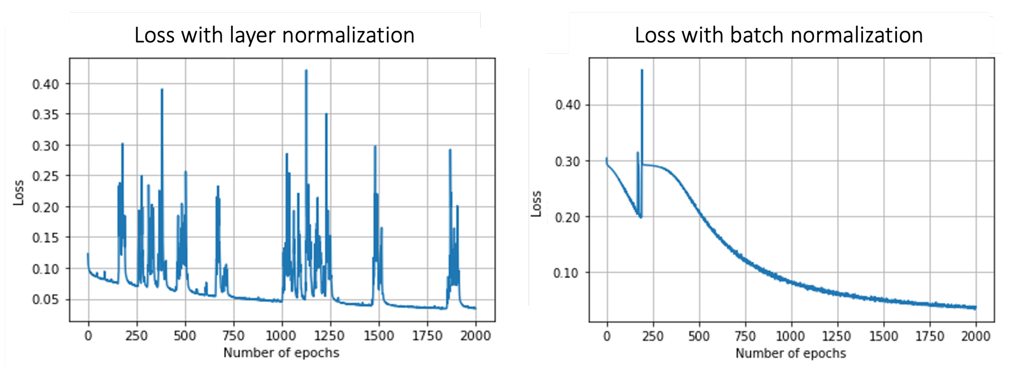
where j is the number of batches that were used for training. The performances of the training with the batch mode and the layer mode are evaluated with the loss over the number of epochs (see Figure 4). Note that the MSE loss function is implemented in the network. As is shown in Figure 4, the batch normalization starts with a higher loss value, but it is reduced over epochs with a smooth curve. In contrast, layer normalization, which normalizes data layer by layer, starts with a lower loss value. However, the value of loss fluctuates throughout the training and results in a jagged learning process. That is because strong IQ signals (e.g., IQ signals around the tornado hook echo) can dominate the learning process over the weak weather IQ signals with layer normalization in the layer mode. This issue can be resolved with the batch mode that adjusts the learning setting for the neural network to keep the consistency of the data along the azimuth pixels. The size of the batch can be equal to the number of transmit beams, so that data over 360 (azimuth) can be normalized together.
Another important training strategy includes the choice of an optimizer. Adaptive Moment Estimation (Adam) is used in a batch mode for the training as an optimizer. Adam is a stochastic gradient descent method that is based on adaptive estimation of the first-order and second-order moments [37]. Adam is one of the most used optimization algorithms for deep learning, because it requires less memory, offers computational efficiency, and is invariant to diagonal re-scaling of the gradients. Therefore, Adam is well suited for training with large data sets. The convergence for the Adam optimizer is analyzed in [38].
The proposed network, ABCNN, was trained within a reasonable time (18 h) with a compact neural network design even though the training data were complex and heavy. Furthermore, preliminary results show that ABCNN successfully mimics the adaptive DBF skills from the Capon method (discussed in the following section). However, CNN often can lead to a limitation of uncertainty and errors, and requires various labeled training data. Therefore, ABCNN has the potential to improve the performance of the neural network itself related to saturation issues, efficient training time, more flexible applications, etc., in the future.

3. Results

This section shows the preliminary results of ABCNN. It was tested with the tornadic supercell storm case from 20 May 2013 at 20:04:14 Z. The performance of DBF by the Capon, Fourier, and ABCNN methods is evaluated in three different areas: storm area, stationary clutters (i.e., SPT), and moving clutters (i.e., WTC). The analysis was performed with qualitative and quantitative metrics. The qualitative metrics are (1) power, plotted in PPI and line plot forms, and (2) antenna patterns resulting from each method. The quality of the overall weather observations with ABCNN can be analyzed with the (1) metrics. Then the half-power beamwidth, sidelobe levels, location of null, and the overall shape of the beam pattern can be analyzed through the (2) metrics. The quantitative metrics are (1) depth of null at the location of clutter, and (2) computation time as a function of the receiver number. The main goal of ABCNN is to mimic the adaptive DBF skills of the Capon method by adaptively placing a null at the location where the clutter is present. Therefore, ABCNN can minimize the overall power and mitigate the contamination from clutter. Moreover, ABCNN is expected to perform adaptive DBF faster than the Capon method.

3.1. Qualitative Analysis

First, the PPI plot of the power by the Capon, Fourier, and ABCNN DBF methods is shown in Figure 5. The power by each DBF method is calculated following Equation (1) with the beamforming weights. They are normalized to have a peak power at 40 dB for ease of comparison with each other and the original NEXRAD data. As is shown in the figure, the Fourier DBF shows serious contamination in the tornado hook echo area due to clutter via sidelobes. This can lead to a serious problem in making an accurate forecast of several storms. On the other hand, the Capon and ABCNN have successfully performed adaptive DBF and suppressed the high power returns coming from the undesired directions to mitigate the contamination. Furthermore, the Capon and ABCNN DBFs produce the same power dynamic, which shows that ABCNN has been trained well to mimic the Capon method.
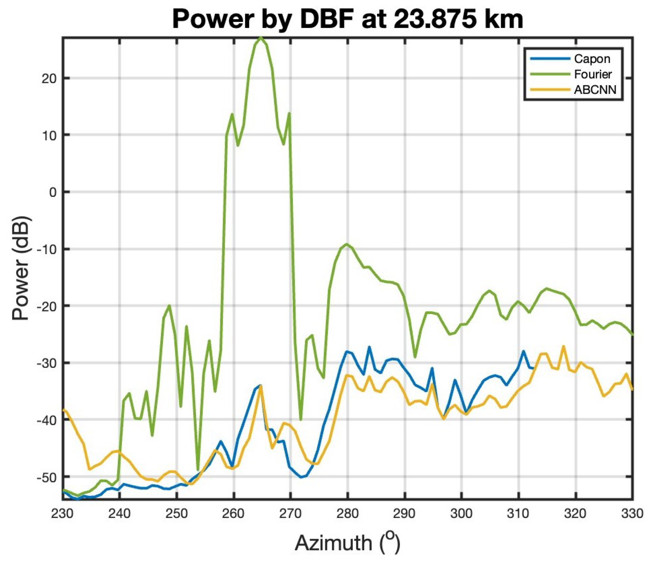
Second, the power of each DBF method at 23.875 km (range) from 230 to 330 is plotted in Figure 6 to evaluate DBF performance in detail. Note that all power plots are normalized to their minimum value for ease of comparison, since they all have different peak values and different dynamic ranges. The wind turbine is located at 264.23 . The Fourier DBF shows high power returns coming back from 255 to 270 , which is caused by sidelobe contamination from the WTC. On the other hand, the Capon and the ABCNN DBFs minimize overall power by suppressing the high power return from the undesired directions. Furthermore, note that the overall trends of the Capon and ABCNN are well-matched. This also shows that ABCNN successfully mimics the behavior of the Capon method.
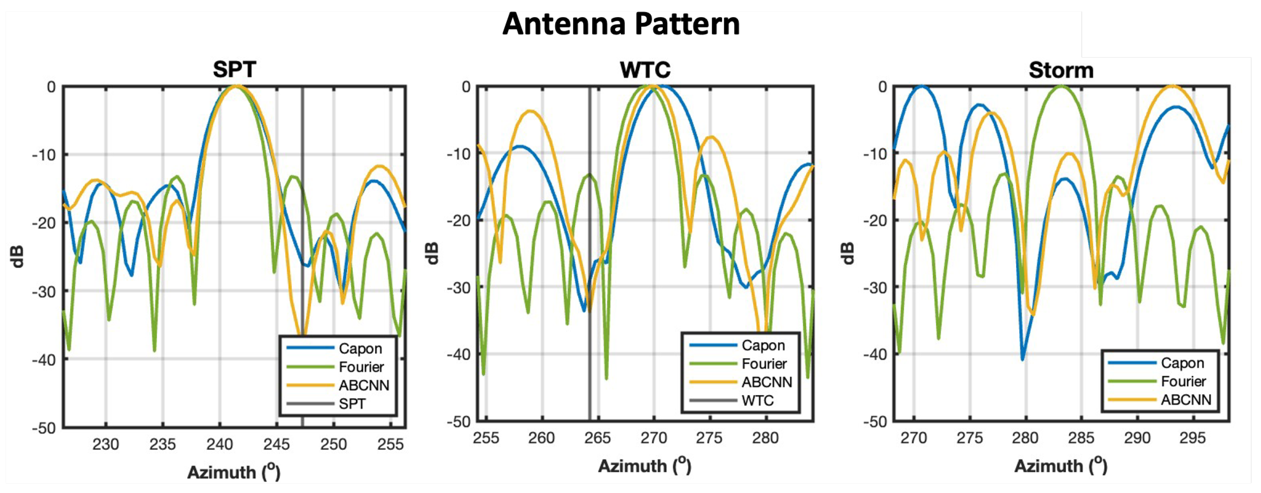
Third, the antenna patterns of each DBF method for three different cases, SPT, WTC, and storm area, are plotted in Figure 7. Note that beam patterns are normalized to have a peak at 0 dB. Antenna patterns directly show the adaptive nulling capability of ABCNN. Furthermore, the similarity between antenna patterns of the Capon and ABCNN shows how well ABCNN is trained to mimic the Capon method. The first case is SPT, plotted in the left plot in Figure 7. Antenna patterns are measured at 241.74 , and the SPT is located at 248.26 , indicated by a gray line. The Fourier method (green) has high sidelobes of −13.45 dB at the location of this clutter, while the Capon (blue) and ABCNN (yellow) place a null and reduce the sidelobe levels to −26.39 dB and −38.45 dB. The second case is WTC, plotted in the middle plot. Antenna patterns are measured at 269.23 , and WTC is located at 264.23 , indicated by a gray line. At the location of WTC, the Fourier has sidelobe levels of −13.18 dB, while the Capon and ABCNN reduce the sidelobe levels to −28.97 dB and −33.76 dB by placing a null at the location of clutter. Lastly, antenna patterns are measured in the storm area shown in the right plot. The beam is pointing at 286.73 . Since the antenna patterns are measured where targets are distributed for this case, there is no specific location where the adaptive DBF methods place a null. However, this case shows that the overall shape of antenna patterns by the Capon and ABCNN method are well matched. Antenna pattern cuts clearly show that the Fourier patterns have been pre-determined from the array geometry and independent from data, which often leads to high sidelobe levels at the location of clutter. Capon and ABCNN successfully placed nulls at the location of the clutter for every case to mitigate the contamination from the clutter targets and minimize the overall power. Furthermore, the overall trends of the Capon and ACBNN antenna patterns are well-matched for all three cases. Therefore, the preliminary qualitative results show that ABCNN has been trained well to mimic the Capon method for both a point target and distributed targets.

3.2. Quantitative Analysis

The depth of null created by adaptive DBF methods at the location of clutter is measured and listed in Table 4. Four antenna patterns pointing at different angles around WTC (264.23 ), and another four antenna patterns pointing at different angles around SPT (247.25 ), are measured. The beam-pointing angles in each case are listed in the third column. As is shown in Table 4, ABCNN always produces a lower power of antenna pattern than the Fourier method at the location of clutter. This shows the benefit of the adaptive DBF by ABCNN over the deterministic DBF by the Fourier method. Furthermore, ABCNN produces a deeper null than the Capon method for the third, fourth, and fifth cases. The third case has WTC at 264.23 , and the beam points at 268.22 . Then, the Capon method places a null with a depth of −30.00 dB, while ABCNN places a null with a depth of −34.56 dB. The fourth case has the same clutter, and the beam points at 269.23 . Again, the Capon method places a null with a depth of −28.97 dB and ABCNN places a null with a depth of −33.76 dB. Lastly, the fifth case has SPT at 247.25 , and the beam points at 241.24 . The Capon has a null with −26.09 dB, while ABCNN has a null with −38.69 dB. This quantitative measurement shows the adaptive nulling ability of the ABCNN method compared with the other two DBF methods.
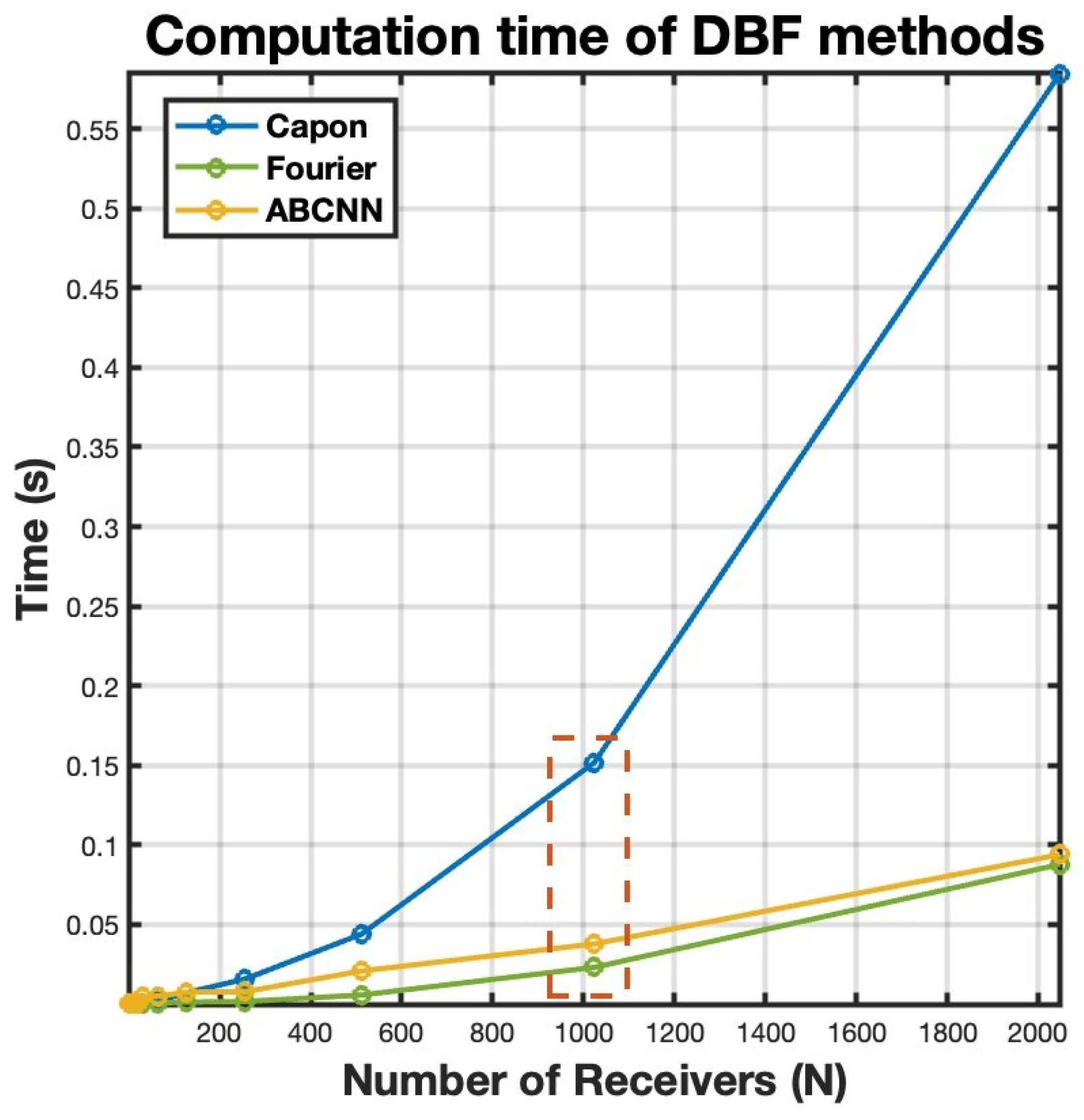
Lastly, the computation time of ABCNN is evaluated. The time to perform DBF for one range gate with six receive beams formed within one transmit beam by each method is measured as a function of the number of receivers, and is illustrated in Figure 8. The simulation of the Capon and Fourier DBFs had been performed in Matlab with an Apple M1 chip processor, and ABCNN was performed in Python with a 2.4 GHz Quad-Core Intel Core i5. The Capon method (blue) shows an exponential growth as the number of receivers increases, while the Fourier (green) and ABCNN (yellow) show a linear growth with the number of receivers. The computation time of ABCNN shows a similar trend and values with the Fourier method. Specifically, ABCNN takes about 0.047 s, and the Capon method takes about 0.15 s to compute beamforming weights of the six receive beams within a transmit beam for one range gate at the size of Horus ( N = 1024 ). This shows that ABCNN lowers computation time by a factor of three compared to the Capon method for one range gate calculation. It can be assumed that the computation of the Capon method will increase exponentially with the number of range gates, while the computation time of ABCNN will increase linearly. Furthermore, the speed of ABCNN can be improved with a faster computer processor. Note that the M1 chip processor is faster than the Intel Core i5 processor in general.

4. Discussion

In this article, CNN has been used to build an algorithm named ABCNN, to perform fast adaptive DBF. The reason CNN has been used for this algorithm is to learn the complex spatial relationship of IQ signals and beamforming weights at each receiver. While the qualitative and quantitative results show that ABCNN has been able to reproduce adaptive DBF by the Capon method without the computational burden, it is important to describe the limitations of the proposed algorithm. CNN requires a lot of labeled training data in order to reduce the various types of uncertainty and errors. In this work, ABCNN was trained with 561 samples extracted from PPI scans. Therefore, the quality of results, their robustness, and their generality can be improved in the future with more labeled training data sets. However, the types of weather may not directly impact the quality of CNN training, since the algorithm takes IQ signals at each range gate without the information of storm type. Instead, more labeled training data may improve the learning process and increase its robustness. Furthermore, different combinations of the neural network components, such as activation functions, types of layers, optimizers, or error functions can be studied in the future, to improve the quality of the CNN engine. Additional ideas for future work are provided in the conclusions.

5. Conclusions and Future Work

The recent development of Horus, a fully digital PAR, enables the possibility of achieving a high temporal resolution for polarimetric weather observations with DBF. The receive beams can be formed with either pre-calculated beamforming weights based on the geometry of the antenna or adaptively calculated beamforming weights based on the received signals at each receiver. The former method produces a fixed shape of the beam pattern, and this often leads to high power returns, which could be caused by clutter or interference from undesired directions. On the other hand, the latter method is a data-dependent process that can place a null at the location of interference to minimize the power from every direction except the desired direction. However, it can be computationally expensive, since it requires more complex mathematics. Furthermore, the complexity order of the data-dependent method (i.e., the Capon method) grows exponentially with the number of receivers, while the data-independent method (i.e., the Fourier method) shows linear growth in the complexity order with the number of receivers.
AI has been widely adopted in various fields and transformed into many different forms to resolve a variety of issues. In this paper, a new fast adaptive DBF method based on deep learning with CNN, named ABCNN, is proposed to overcome the computational burden of the adaptive DBF method while preserving the high data quality. ABCNN is a neural network that was trained with the amplitude and phase of time-series IQ signals and beamforming weights by the Capon method as input and output. Therefore, ABCNN was able to perform adaptive DBF directly from the time-series IQ signals without losing the phase information. Details of training data preparation and training strategy are discussed in Section 2.3.
Preliminary results show the potential that ABCNN can be used for real-time adaptive DBF. The performance of ABCNN was compared with the Capon and the Fourier methods in Section 3. The power PPI scan reconstructed by each DBF was compared with the original NEXRAD data to evaluate the performance of each DBF method. The Fourier method shows significant contamination on the tornado hook echo area due to ground clutter targets, which could lead to the misidentification of severe storms. On the other hand, the Capon and ABCNN methods were able to mitigate both stationary targets (i.e., SPT) and moving targets (i.e., WTC). Antenna patterns generated by the ABCNN method show its capability in terms of adaptive DBF skills (i.e., placing a null at the interference location). Not only that, the general structure of the mainlobe and sidelobes of the Capon and ABCNN methods were well matched, proving that ABCNN was able to learn the behavior of the Capon method through the training. Lastly, the performance of ABCNN was evaluated with a quantitative metric such as computation time. The Capon method shows exponential growth in computation time as the number of receivers grows. Therefore, performing adaptive DBF in real-time with the Capon method becomes challenging. However, ABCNN has successively reduced the computation time to perform adaptive DBF. The computation time of ABCNN shows linear growth as the number of digital receivers increases, which was similar to the computation time to perform the deterministic DBF by the Fourier method.
To conclude the work, ABCNN was successfully trained to perform adaptive DBF by mimicking the behavior of the Capon method for the stationary point target, moving clutter (i.e., WTC), and distributed targets (i.e., weather). It shows the potential to overcome the computational burden of adaptive DBF and permit real-time implementation. The computation time was more than three times faster than the Capon method, and similar to the Fourier method at the specific size of Horus. Furthermore, the training of ABCNN was faster and produced better quality beam patterns compared to existing DL adaptive DBF methods. However, as mentioned throughout the paper, the main contribution of this work is focused on reducing the computational burden of the adaptive DBF methods. Therefore, ABCNN can be improved furthermore to have more efficient training in the future. Another future work can be the enhancement and improvement of the adaptive DBF quality. For example, the network can be trained with multiple inputs, the location of targets and interference, or the steering angle of the antenna to perform adaptive DBF without mimicking the specific existing adaptive methods. Another future effort can involve expanding ABCNN to include information related to the physical properties of the observed hydrometeors, such as the correlation coefficient, differential reflectivity, or velocity, to operate as a hydrometeor classification. Lastly, ABCNN can learn to predict the movement of storms.

Author Contributions

Conceptualization, Y.-S.K., D.S., T.-Y.Y. and R.D.P.; Methodology, Y.-S.K., D.S., T.-Y.Y. and R.D.P.; Software, Y.-S.K.; Validation, D.S., T.-Y.Y. and R.D.P.; Resources, D.S.; Writing—original draft, Y.-S.K.; Writing—review and editing, D.S., T.-Y.Y. and R.D.P.; Visualization, Y.-S.K.; Supervision, D.S., T.-Y.Y. and R.D.P. All authors have read and agreed to the published version of the manuscript.

Funding

This research received no external funding.

Data Availability Statement

The data are available upon request from the corresponding author.

Conflicts of Interest

The authors declare no conflict of interest.

References

  1. Zrnic, D.; Kimpel, J.; Forsyth, D.; Shapiro, A.; Crain, G.; Ferek, R.; Heimmer, J.; Benner, W.; McNellis, F.T.; Vogt, R. Agile-beam phased array radar for weather observations. Bull. Am. Meteorol. Soc. 2007, 88, 1753–1766. [Google Scholar] [CrossRef]
  2. Palmer, R.D.; Bodine, D.; Kollias, P.; Schvartzman, D.; Zrnić, D.; Kirstetter, P.; Zhang, G.; Yu, T.; Kumjian, M.; Cheong, B.; et al. A Primer on Phased Array Radar Technology for the Atmospheric Sciences. Bull. Am. Meteorol. Soc. 2022, 103, E2391–E2416. [Google Scholar] [CrossRef]
  3. Schvartzman, D. Signal Processing Techniques and Concept of Operations for Polarimetric Rotating Phased Array Radar. Ph.D. Thesis, The University of Oklahoma, Norman, OK, USA, 2020. [Google Scholar]
  4. Isom, B.; Palmer, R.; Kelley, R.; Meier, J.; Bodine, D.; Yeary, M.; Cheong, B.L.; Zhang, Y.; Yu, T.Y.; Biggerstaff, M.I. The atmospheric imaging radar: Simultaneous volumetric observations using a phased array weather radar. J. Atmos. Ocean. Technol. 2013, 30, 655–675. [Google Scholar] [CrossRef]
  5. Palmer, R.D.; Yeary, M.B.; Schvartzman, D.; Salazar-Cerreno, J.L.; Fulton, C.; McCord, M.; Cheong, B.; Bodine, D.; Kirstetter, P.; Sigmarsson, H.H.; et al. Horus—A Fully Digital Polarimetric Phased Array Radar for Next-Generation Weather Observations. IEEE Trans. Radar Syst. 2023, 1, 96–117. [Google Scholar] [CrossRef]
  6. Hondl, K.; Weber, M. NOAA’s Meteorological Phased Array Radar Research Program. In Proceedings of the 2019 IEEE International Symposium on Phased Array System & Technology (PAST), Waltham, MA, USA, 15–18 October 2019; IEEE: Piscataway, NJ, USA, 2019; pp. 1–6. [Google Scholar]
  7. Palmer, R.D.; Gopalam, S.; Yu, T.Y.; Fukao, S. Coherent radar imaging using Capon’s method. Radio Sci. 1998, 33, 1585–1598. [Google Scholar] [CrossRef]
  8. Yu, T.Y.; Palmer, R.D.; Hysell, D.L. A simulation study of coherent radar imaging. Radio Sci. 2000, 35, 1129–1141. [Google Scholar] [CrossRef]
  9. Mahmoud, K.R.; Eladawy, M.I.; Bansal, R.; Zainud-Deen, S.H.; Ibrahem, S.M. Analysis of uniform circular arrays for adaptive beamforming applications using particle swarm optimization algorithm. Int. J. RF Microw. Comput.-Aided Eng. 2008, 18, 42–52. [Google Scholar] [CrossRef]
  10. Zaman, M.A.; Abdul Matin, M. Nonuniformly spaced linear antenna array design using firefly algorithm. Int. J. Microw. Sci. Technol. 2012, 2012, 256759. [Google Scholar] [CrossRef]
  11. Lu, Y.; Yeo, B.K. Adaptive wide null steering for digital beamforming array with the complex coded genetic algorithm. In Proceedings of the 2000 IEEE International Conference on Phased Array Systems and Technology (Cat. No. 00TH8510), Dana Point, CA, USA, 21–25 May 2000; IEEE: Piscataway, NJ, USA, 2000; pp. 557–560. [Google Scholar]
  12. McGovern, A.; Lagerquist, R.; Gagne, D.J.; Jergensen, G.E.; Elmore, K.L.; Homeyer, C.R.; Smith, T. Making the black box more transparent: Understanding the physical implications of machine learning. Bull. Am. Meteorol. Soc. 2019, 100, 2175–2199. [Google Scholar] [CrossRef]
  13. Carbonell, J.G.; Michalski, R.S.; Mitchell, T.M. An overview of machine learning. Mach. Learn. 1983, 1, 3–23. [Google Scholar]
  14. LeCun, Y.; Bengio, Y.; Hinton, G. Deep learning. Nature 2015, 521, 436–444. [Google Scholar] [CrossRef] [PubMed]
  15. Luijten, B.; Cohen, R.; de Bruijn, F.J.; Schmeitz, H.A.; Mischi, M.; Eldar, Y.C.; van Sloun, R.J. Adaptive ultrasound beamforming using deep learning. IEEE Trans. Med. Imaging 2020, 39, 3967–3978. [Google Scholar] [CrossRef] [PubMed]
  16. Jalal, B.; Yang, X.; Liu, Q.; Long, T.; Sarkar, T.K. Fast and robust variable-step-size LMS algorithm for adaptive beamforming. IEEE Antennas Wirel. Propag. Lett. 2020, 19, 1206–1210. [Google Scholar] [CrossRef]
  17. Sallam, T.; Abdel-Rahman, A.B.; Alghoniemy, M.; Kawasaki, Z.; Ushio, T. A neural-network-based beamformer for phased array weather radar. IEEE Trans. Geosci. Remote Sens. 2016, 54, 5095–5104. [Google Scholar] [CrossRef]
  18. Kim, Y.S.; Schvartzman, D.; Palmer, R.D.; Yu, T.Y. Fast Adaptive Beamforming Using Deep Learning for Digital Phased Array Radars. In Proceedings of the 2022 IEEE International Symposium on Phased Array Systems & Technology (PAST), Waltham, MA, USA, 11–14 October 2022; IEEE: Piscataway, NJ, USA, 2022; pp. 1–7. [Google Scholar]
  19. Barrachina, J.A. NEGU93/cvnn: Complex-Valued Neural Networks. Ph.D. Thesis, Université Paris-Saclay, Paris, France, 2022. [Google Scholar]
  20. Gulli, A.; Pal, S. Deep Learning with Keras; Packt Publishing Ltd.: Birmingham, UK, 2017. [Google Scholar]
  21. Chollet, F. Keras. 2015. Available online: https://github.com/fchollet/keras (accessed on 20 December 2022).
  22. Adachi, T.; Mashiko, W. High temporal-spatial resolution observation of tornadogenesis in a shallow supercell associated with Typhoon Hagibis (2019) using phased array weather radar. Geophys. Res. Lett. 2020, 47, e2020GL089635. [Google Scholar] [CrossRef]
  23. Schvartzman, D.; Torres, S.M.; Yu, T.Y. Distributed Beams: Concept of Operations for Polarimetric Rotating Phased Array Radar. IEEE Trans. Geosci. Remote Sens. 2021, 59, 9173–9191. [Google Scholar] [CrossRef]
  24. Bluestein, H.B.; Rauber, R.M.; Burgess, D.W.; Albrecht, B.; Ellis, S.M.; Richardson, Y.P.; Jorgensen, D.P.; Frasier, S.J.; Chilson, P.; Palmer, R.D.; et al. Radar in atmospheric sciences and related research: Current systems, emerging technology, and future needs. Bull. Am. Meteorol. Soc. 2014, 95, 1850–1861. [Google Scholar] [CrossRef]
  25. Van Trees, H.L. Optimum Array Processing: Part IV of Detection, Estimation, and Modulation Theory; John Wiley & Sons: Hoboken, NJ, USA, 2004. [Google Scholar]
  26. Capon, J. High-resolution frequency-wavenumber spectrum analysis. Proc. IEEE 1969, 57, 1408–1418. [Google Scholar] [CrossRef]
  27. Luenberger, D.G.; Ye, Y. Linear and Nonlinear Programming; Springer: Berlin/Heidelberg, Germany, 1984; Volume 2. [Google Scholar]
  28. Du, D.Z.; Ko, K.I. Theory of Computational Complexity; John Wiley & Sons: Hoboken, NJ, USA, 2011; Volume 58. [Google Scholar]
  29. Zrnic, D. Simulation of weatherlike Doppler spectra and signals. J. Appl. Meteorol. Climatol. 1975, 14, 619–620. [Google Scholar] [CrossRef]
  30. Schvartzman, D.; Curtis, C.D. Signal processing and radar characteristics (SPARC) simulator: A flexible dual-polarization weather-radar signal simulation framework based on preexisting radar-variable data. IEEE J. Sel. Top. Appl. Earth Obs. Remote Sens. 2018, 12, 135–150. [Google Scholar] [CrossRef]
  31. Helmus, J.J.; Collis, S.M. The Python ARM Radar Toolkit (Py-ART), a library for working with weather radar data in the Python programming language. J. Open Res. Softw. 2016, 4, e25. [Google Scholar] [CrossRef]
  32. Schvartzman, D.; Palmer, R.; Yu, T.Y.; Reinke, R.; Nai, F. A Pattern Synthesis Method for Polarimetric Weather Observations with the All-Digital Horus Phased Array Radar. In Proceedings of the 102nd American Meteorological Society Annual Meeting, Houston, TX, USA, 23–27 January 2022; AMS: Boston, MA, USA, 2022. [Google Scholar]
  33. Richards, M.A. Fundamentals of Radar Signal Processing; McGraw-Hill Education: New York, NY, USA, 2014. [Google Scholar]
  34. Schvartzman, D. Mitigation of Wind Turbine Clutter With Digital Phased Array Radar. IEEE Access 2023, 11, 12911–12924. [Google Scholar] [CrossRef]
  35. Szandała, T. Review and comparison of commonly used activation functions for deep neural networks. In Bio-Inspired Neurocomputing; Springer: Berlin/Heidelberg, Germany, 2021; pp. 203–224. [Google Scholar]
  36. Ioffe, S.; Szegedy, C. Batch normalization: Accelerating deep network training by reducing internal covariate shift. In Proceedings of the International Conference on Machine Learning, Lille, France, 6–11 July 2015; PMLR: Westminster, UK, 2015; pp. 448–456. [Google Scholar]
  37. Kingma, D.P.; Ba, J. Adam: A method for stochastic optimization. arXiv 2014, arXiv:1412.6980s. [Google Scholar]
  38. Bock, S.; Weiß, M. A proof of local convergence for the Adam optimizer. In Proceedings of the 2019 International Joint Conference on Neural Networks (IJCNN), Budapest, Hungary, 14–19 July 2019; IEEE: Piscataway, NJ, USA, 2019; pp. 1–8. [Google Scholar]
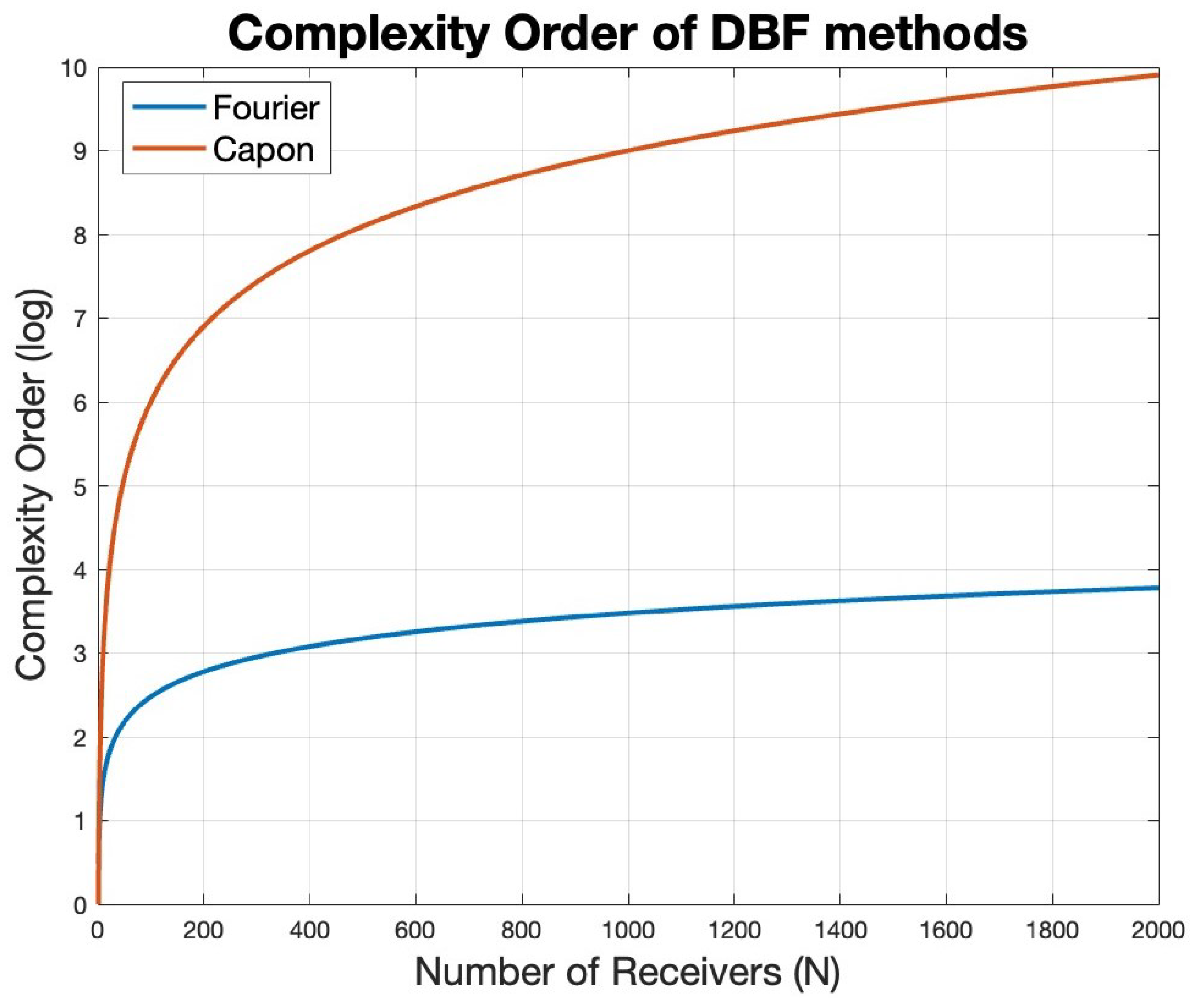
Figure 1. Complexity order in the logarithm scale of the Fourier and the Capon methods as a function of receiver number is shown above. The blue line represents the complexity order of the Fourier method, and the red line represents the complexity order of the Capon method.
Remotesensing 15 04129 g001
Figure 2. Plane-position indicator (PPI) scan of the simulated model power (dB) from the tornadic storm case observed on 20 May 2013 20:03:56.96 by the NEXRAD KTLX radar. There are a total of 8 wind turbines and 4 stationary point targets; their locations are listed in Table 3 and are represented by red dots in the figure.
Remotesensing 15 04129 g002
Figure 3. Training process and architecture of ABCNN is shown. It takes complex-valued time-series signals, separates the complex values into polar forms, learns phase and amplitude information of time-series signals independently in parallel, and produces phase and amplitude values for beamforming weights as a function of beam pointing direction in azimuth ( ϕ ) and receivers (N). Each layer in the architecture is colored differently and listed.
Remotesensing 15 04129 g003
Figure 4. Loss during the training with the batch normalization (right) and layer normalization (left) with MSE loss function is shown above. The x-axis represents the number of epochs and the y-axis represents the loss value.
Remotesensing 15 04129 g004
Figure 5. The PPI plot of signal power (dB) for the Capon (left), the Fourier (middle), and ABCNN (right) methods is shown. Note that all signal power fields are normalized to have a peak at 40 dB. The PPI plot for the Fourier DBF has a color scale from −42 dB to 40 dB and the Capon and ABCNN have a color scale from −2 dB to 40 dB.
Remotesensing 15 04129 g005
Figure 6. Signal power by the Capon (blue), the Fourier (green), and ABCNN (yellow) DBF methods at 23.875 km (range) from 230 to 330 is shown. The wind turbine is located at 264.23 .
Remotesensing 15 04129 g006
Figure 7. Antenna pattern cuts of the Capon (blue), the Fourier (green), and ABCNN (yellow) methods for three different cases are plotted. First, the left plot shows the SPT case. The SPT is located at 23.625 km and 248.26 (gray line) and the beam is pointing at 241.74 . The second case is the WTC, shown in the middle plot. The WTC is located at 21.625 km and 264.23 and the beam is pointing at 269.23 . Lastly, antenna patterns are measured at the storm area shown in the right plot. The beam is pointing at 286.73 .
Remotesensing 15 04129 g007
Figure 8. The computation time of the Capon method (blue), the Fourier method (green), and ABCNN (yellow) to generate 6 receive beams within a transmit beam for one range gate as a function of receiver number (N) is shown. The size for Horus (1024) is marked with a red dotted box. At the size of Horus, ABCNN is more than three times faster compared to the Capon method.
Remotesensing 15 04129 g008
Table 1. Review of adaptive digital beamforming with AI methods.
Name of AlgorithmAI TypeInputOutputCharacteristics
ABLEDL with Dense layersReal and Imaginary parts of IQ signalsDownstream systemLearning process can be heavy, and it may result in saturation easily due to dense layers
Fast and Robust VSS-LMSLSMReceived and reference signalsArray patternsLower complexity of the neural network
RBFNNDLReal and Imaginary parts of covariance matrixReal and Imaginary parts of inversed covaraince matrixDoubled length of the network due to complex value separation
DLAFDL with Dense layersComplex valued IQ signalsComplex valued beamforming weightsEasy saturation during the training and lack of flexibility of network and training due to the limited library
ABCNNCNNPhase and amplitude of IQ signalsPhase and amplitude of beamforming weightsPreserves phase information and learns the spatial relation in data
Table 2. Parameters used in digital PAR simulation for weather data are shown below.
ParameterValues
Operation Frequency (f)3 GHz (S-band)
Range resolution250 m
Number of antenna element (N)32
Spacing (d)16.4 mm
Number of sample (M)64
Range coverage0.125 km–35.125 km
Azimuth coverage0 –360
Table 3. Types and location of clutter targets are listed below.
TypeRange (km)Azimuth ( )
SPT20.375247.25
SPT23.625248.26
SPT25.375279.74
SPT27.375277.24
WTC21.625264.23
WTC22.125263.23
WTC22.625261.76
WTC23.125260.76
WTC23.625259.26
WTC24.375259.26
WTC25.125259.26
WTC26.125259.26
Table 4. Sidelobe levels of antenna patterns by each DBF method are measured and listed below.
Clutter TypeClutter Location ( )Pointing Angle ( )Capon (dB)Fourier (dB)ABCNN (dB)
WTC264.23263.23−28.53−1.03−26.82
WTC264.23265.25−16.04−1.04−16.04
WTC264.23268.22−30.00−19.56−34.56
WTC264.23269.23−28.97−13.18−33.76
SPT247.25241.24−26.09−15.23−38.69
SPT247.25246.18−20.09−1.02−20.09
SPT247.25253.24−28.71−16.52−24.83
SPT247.25255.18−27.93−20.18−25.54
Disclaimer/Publisher’s Note: The statements, opinions and data contained in all publications are solely those of the individual author(s) and contributor(s) and not of MDPI and/or the editor(s). MDPI and/or the editor(s) disclaim responsibility for any injury to people or property resulting from any ideas, methods, instructions or products referred to in the content.