
Improving the Pulse-Limited Footprint Resolution of GNSS-R Based on the Novel Joint Bandwidth Method

 ,
,
Abstract
:
1. Introduction
2. Methods
2.1. Size of Pulse-Limited Footprint
2.2. Galileo/GNSS-R NJBW Method
2.3. Pulse-Limited Footprint of the Galileo/GNSS-R E5a/b NJBW Joint Signal
3. Results and Discussion
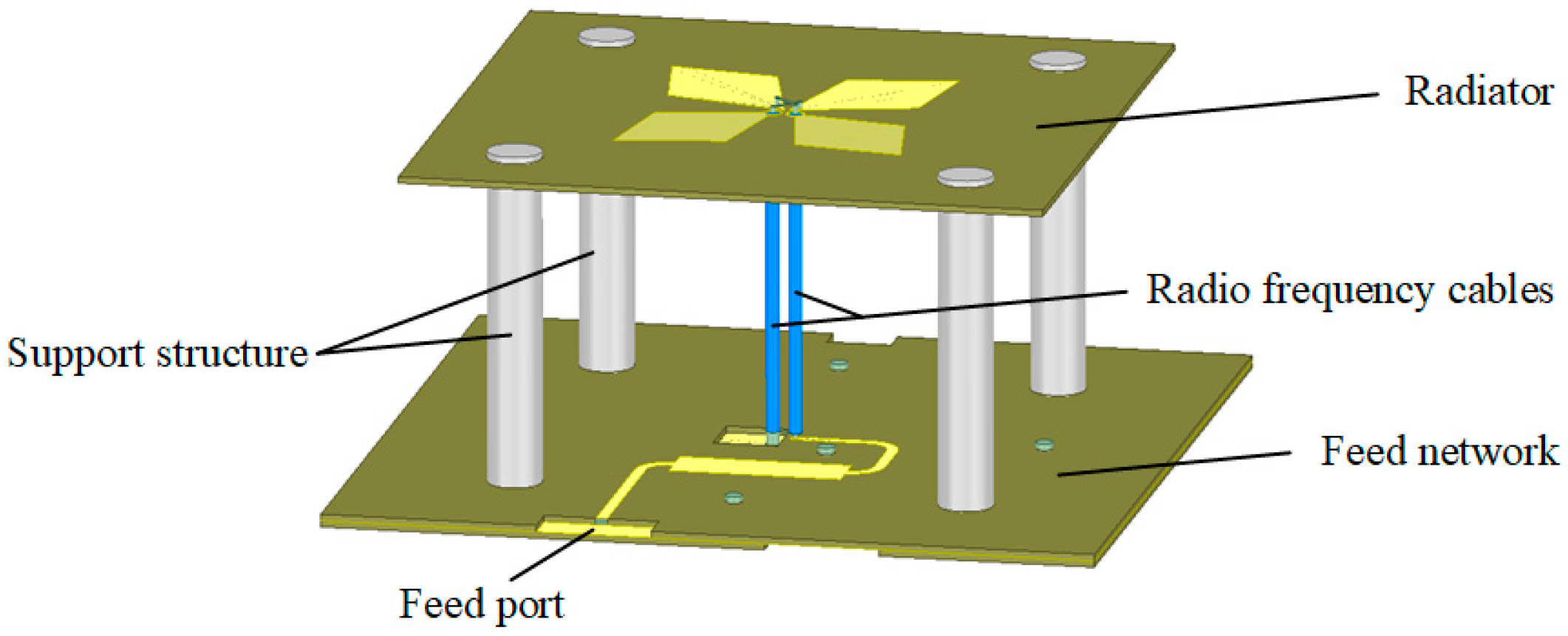
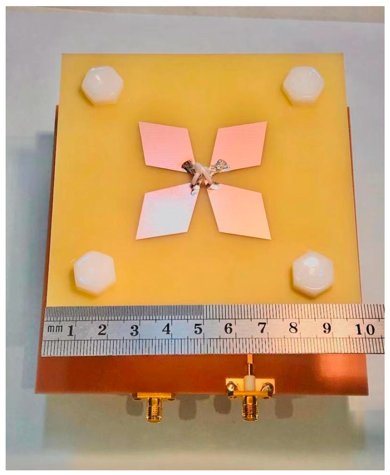
3.1. Design of the E5a/b NJBW Antenna Verification Prototype
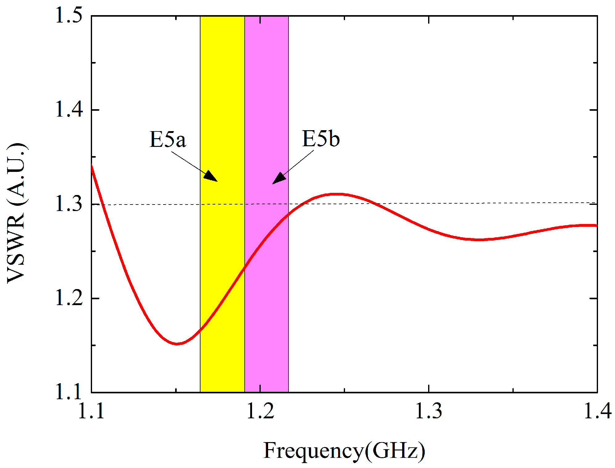
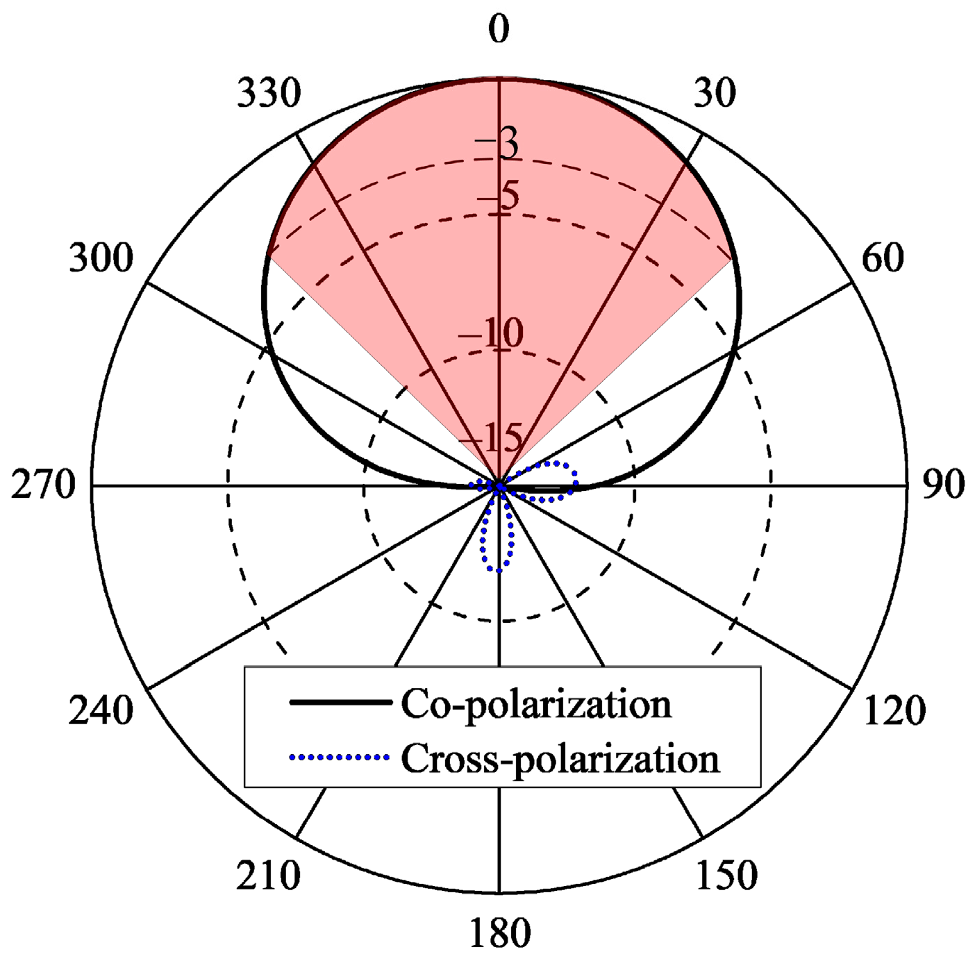
3.2. Testing of the E5a/b NJBW Antenna Verification Prototype
3.3. Resolution of the E5a/b NJBW Joint Signal
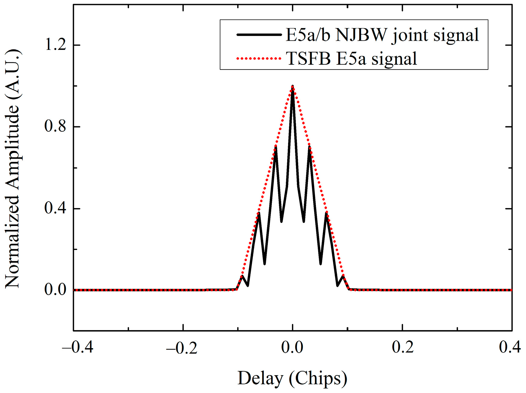
3.3.1. Main Lobe Width of ACF
3.3.2. Pulse-Limited Footprint Resolution
4. Conclusions
- (1)
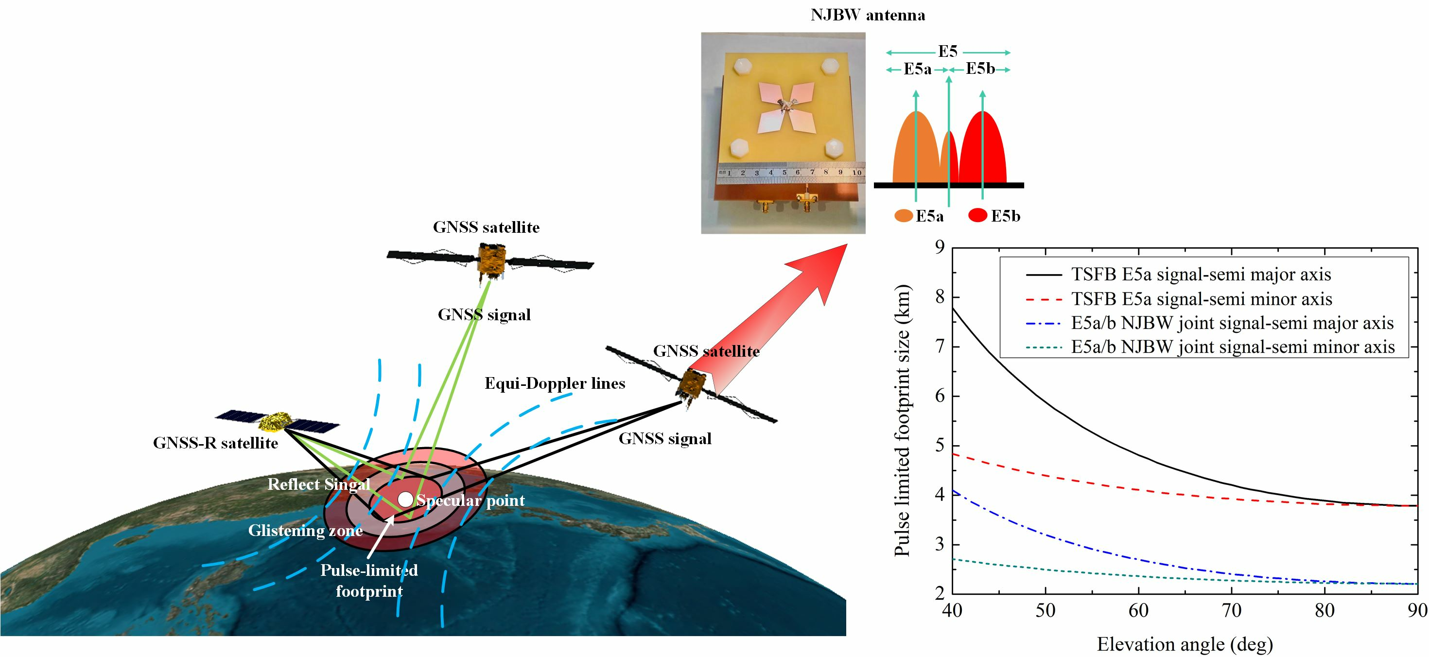
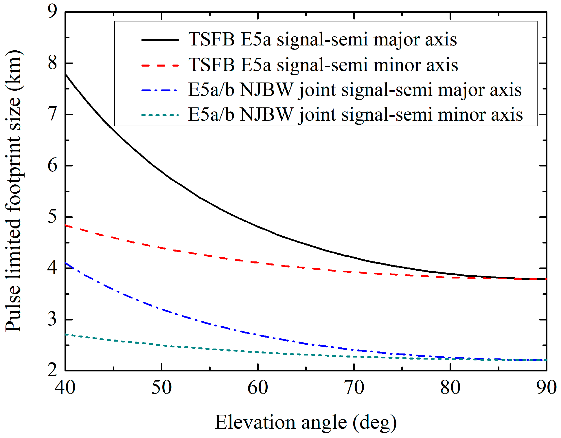
- In order to reduce the pulse-limited footprint size and improve the pulse-limited footprint resolution, we propose a NJBW method of jointing Galileo E5a and E5b reflected signal bandwidth based on the GNSS-R auto-correlation signal ambiguity theory. This method reduces the ACF width of the GNSS-R signal by jointing the E5a and E5b frequency bands, thereby improving the pulse-limited footprint resolution of Galileo/GNSS-R. For the Galileo E5a/b NJBW joint signal, the main lobe width of its ACF is 1/3 of that of the TSFB E5a signal, its pulse-limited footprint size is of that of the TSFB E5a signal, and the pulse-limited footprint resolution is increased by about 1.73 times.
- (2)
- In order to verify the Galileo/GNSS-R NJBW method, this article designed and fabricated a Galileo/GNSS-R E5a/b NJBW antenna verification prototype. The performance of the E5a/b NJBW antenna verification prototype meets the requirements for applying in the E5a and E5b frequency bands, effectively expanding the bandwidth of the Galileo/GNSS-R RF channel and effectively expanding the Galileo/GNSS-R processed signal bandwidth. According to the tested results of the E5a/b NJBW antenna verification prototype, compared with the TSFB E5a signal, the E5a/b NJBW joint signal can reduce the pulse-limited footprint size from 3.8 km to 2.2 km, and the footprint resolution is increased by 1.72 times, which is very close to the theoretical result of the model.
- (3)
- According to the tested results of the Galileo/GNSS-R E5a/b NJBW antenna verification prototype, it is shown that applying the NJBW method can improve the fineness of the Galileo/GNSS-R pulse-limited footprint size and then improve the pulse-limited footprint resolution. The Galileo E5a/b NJBW method proposed in this paper provides a theoretical method basis and key technical support for the wind field retrieval and height retrieval and antenna design of the GNSS-R sea surface wind field retrieval and height retrieval verification satellite with high pulse-limited footprint resolution in the future.
Author Contributions
Funding
Data Availability Statement
Conflicts of Interest
References
- Martin-Neira, M. A passive reflectometry and interferometry system (PARIS): Application to ocean altimetry. ESA J. 1993, 17, 331–355. [Google Scholar]
- Katzberg, S.J.; Garrison, J.L. Utilizing GPS to determine ionospheric delay over the ocean. In NASA Technical Memo; NASA Center for Aerospace Information: Linthicum Heights, MD, USA, 1996. [Google Scholar]
- Garrison, J.L.; Katzberg, S.J. Detection of ocean reflected GPS signals: Theory and experiment. In Proceedings of the IEEE SOUTHEASTCON’97, Blacksburg, VA, USA, 12–14 April 1997. [Google Scholar]
- Garrison, J.L.; Katzberg, S.J.; Hill, M.I. Effect of sea roughness on bistatically scattered range coded signals from the Global Positioning System. Geophys. Res. Lett. 1998, 25, 2257–2260. [Google Scholar] [CrossRef]
- Shaw, P.T.; Chao, S.Y.; Fu, L.L. Sea surface height variations in the South China Sea from satellite altimetry. Oceanol. Acta 1999, 22, 1–17. [Google Scholar] [CrossRef]
- Shum, C.; Yi, Y.; Cheng, K.; Kuo, C.; Braun, A.; Calmant, S.; Chambers, D. Calibration of JASON-1 altimeter over lake erie special issue: Jason-1 calibration/validation. Mar. Geod. 2003, 26, 335–354. [Google Scholar] [CrossRef]
- Hausleitner, W.; Moser, F.; Desjonqueres, J.D.; Boy, F.; Picot, N.; Weingrill, J.; Mertikas, S.; Daskalakis, A. A new method of precise Jason-2 altimeter calibration using a microwave transponder. Mar. Geod. 2012, 35, 337–362. [Google Scholar] [CrossRef]
- Maiwald, F.; Montes, O.; Padmanabhan, S.; Michaels, D.; Kitiyakara, A.; Jarnot, R.; Brown, S.T.; Dawson, D.; Wu, A.; Hatch, W.; et al. Reliable and stable radiometers for Jason-3. IEEE J. Sel. Top. Appl. Earth Obs. Remote Sens. 2016, 9, 2754–2762. [Google Scholar] [CrossRef]
- Auber, J.C.; Bibaut, A.; Rigal, J.M. Characterization of multipath on land and sea at GPS frequencies. In Proceedings of the 7th International Technical Meeting of the Satellite Division of the Institute of Navigation (ION GPS 1994), Salt Lake City, UT, USA, 20–23 September 1994. [Google Scholar]
- Lin, B.; Katzberg, S.J.; Garrison, J.L.; Wielick, B.A. The relationship between the GPS signals reflected from sea surface and the surface winds: Modeling results and comparisons with aircraft measurements. J. Geophys. Res. Oceans 1999, 104, 20713–20727. [Google Scholar] [CrossRef]
- Garrison, J.L.; Katzberg, S.J. The application of reflected GPS signals to ocean remote sensing. Remote Sens. Environ. 2000, 73, 175–187. [Google Scholar] [CrossRef]
- Katzberg, S.J.; Walker, R.A.; Roles, J.H.; Lynch, T.; Black, P.G. First GPS signals reflected from the interior of a tropical storm: Preliminary results from Hurricane Michael. Geophys. Res. Lett. 2001, 28, 1981–1984. [Google Scholar] [CrossRef]
- Elfouhaily, T.; Chapron, B.; Katsaros, K.; Vandemark, D. A unified directional spectrum for long and short wind-driven waves. J. Geophys. Res. Ocean. 1997, 102, 15781–15796. [Google Scholar] [CrossRef]
- Zavorotny, V.U.; Voronovich, A.G. Scattering of GPS signals from the ocean with wind remote sensing application. IEEE Trans. Geosci. Remote Sens. 2000, 38, 951–964. [Google Scholar] [CrossRef]
- Hajj, G.A.; Zuffada, C. Theoretical description of a bistatic system for ocean altimetry using the GPS signal. Radio Sci. 2003, 38, 1–19. [Google Scholar] [CrossRef]
- Valencia, E.; Camps, A.; Marchan-Hernandez, J.F.; Hyuk, P.; Bosch-Lluis, X.; Rodriguez-Alvarez, N.; Ramos-Perez, I. Ocean surface’s scattering coefficient retrieval by delay–Doppler map inversion. IEEE Geosci. Remote Sens. Lett. 2011, 8, 750–754. [Google Scholar] [CrossRef]
- Gleason, S.; Hodgart, S.; Sun, Y.; Gommenginger, C.; Mackin, S.; Adjrad, M.; Unwin, M. Detection and processing of bistatically reflected GPS signals from low earth orbit for the purpose of ocean remote sensing. IEEE Trans. Geosci. Remote Sens. 2005, 43, 1229–1241. [Google Scholar] [CrossRef]
- Li, C.; Huang, W. An algorithm for sea-surface wind field retrieval from GNSS-R delay-Doppler map. IEEE Geosci. Remote Sens. Lett. 2014, 11, 2110–2114. [Google Scholar]
- Clarizia, M.P.; Ruf, C.S.; Jales, P.; Gommenginger, C. Spaceborne GNSS-R minimum variance wind speed estimator. IEEE Trans. Geosci. Remote Sens. 2014, 52, 6829–6843. [Google Scholar] [CrossRef]
- Zheng, W.; Xu, H.; Zhong, M.; Yun, M. Improvement in the recovery accuracy of the lunar gravity field based on the future Moon-ILRS spacecraft gravity mission. Surv. Geophys. 2015, 36, 587–619. [Google Scholar] [CrossRef]
- Wu, F.; Zheng, W.; Li, Z.; Liu, Z. Improving the GNSS-R specular reflection point positioning accuracy using the gravity field normal projection reflection reference surface combination correction method. Remote Sens. 2019, 11, 33. [Google Scholar] [CrossRef]
- Wu, F.; Zheng, W.; Li, Z.; Liu, Z. Improving the positioning accuracy of satellite-borne GNSS-R specular reflection point on sea surface based on the ocean tidal time-varying elevation correction positioning method. Remote Sens. 2019, 11, 1626. [Google Scholar] [CrossRef]
- Liu, Z.; Zheng, W.; Wu, F.; Li, X.; Zhu, C.; Liu, Z.; Ma, X. Improving the number of sea surface altimetry reflected signals received by GNSS-R satellite based on the new satellite-borne nadia antenna receiving signal-to-noise ratio model. Remote Sens. 2019, 11, 1–16. [Google Scholar]
- Wu, F.; Zheng, W.; Liu, Z.; Sun, X. Improving the specular point positioning accuracy of ship-borne GNSS-R observations in China’s Seas based on a new instantaneous sea reflection surface model. Front. Earth Sci. 2021, 9, 662-1–662-11. [Google Scholar] [CrossRef]
- Cui, Z.; Zheng, W.; Wu, F.; Kang, G.; Li, Z.; Wang, Q.; Cui, Z. Improving GNSS-R sea surface altimetry precision based on the novel dual circularly polarized phased array antenna model. Remote Sens. 2021, 13, 2974. [Google Scholar] [CrossRef]
- Wang, Q.; Zheng, W.; Wu, F.; Xu, A.; Zhu, H.; Liu, Z. A new GNSS-R altimetry algorithm based on machine learning fusion model and feature optimization to improve the precision of sea surface height retrieval. Front. Earth Sci. 2021, 9, 758. [Google Scholar] [CrossRef]
- Sun, X.; Zheng, W.; Wu, F.; Liu, Z. Improving the iGNSS-R ocean altimetric precision based on the coherent integration time optimization Model. Remote Sens. 2021, 13, 4715. [Google Scholar] [CrossRef]
- Liu, Z.; Zheng, W.; Wu, F.; Kang, G.; Sun, X.; Wang, Q. Relationship between altimetric quality and along-track spatial resolution for iGNSS-R sea surface altimetry: Example for the airborne experiment. Front. Earth Sci. 2021, 9, 1119. [Google Scholar] [CrossRef]
- Yan, Z.; Zheng, W.; Wu, F.; Wang, C.; Zhu, H.; Xu, A. Correction of atmospheric delay error of airborne and spaceborne GNSS-R sea surface altimetry. Front. Earth Sci. 2022, 10, 730551. [Google Scholar] [CrossRef]
- Wang, Q.; Zheng, W.; Wu, F.; Zhu, H.; Xu, A.; Shen, Y.; Zhao, Y. Improving the SSH retrieval precision of spaceborne GNSS-R based on a new grid search multihidden layer neural network feature optimization method. Remote Sens. 2022, 14, 3161. [Google Scholar] [CrossRef]
- Zavorotny, V.U.; Gleason, S.; Cardellach, E.; Camps, A. Tutorial on remote sensing using GNSS bistatic radar of opportunity. IEEE Geosci. Remote Sens. Mag. 2014, 2, 8–45. [Google Scholar] [CrossRef]
- Unwin, M.; Gleason, S.; Brennan, M. The space GPS reflectometry experiment on the UK disaster monitoring constellation satellite. In Proceedings of the 16th International Technical Meeting of the Satellite Division of The Institute of Navigation (ION GPS/GNSS 2003), Portland, OR, USA, 9–12 September 2003. [Google Scholar]
- Jales, P.; Unwin, M. MERRByS Product Manual: GNSS Reflectometry on TDS-1 with the SGR-ReSI; Surrey Satellite Technology Ltd.: Guildford, UK, 2017. [Google Scholar]
- Carreno-Luengo, H.; Camps, A.; Via, P.; Munoz, J.F.; Cortiella, A.; Vidal, D.; Jane, J.; Catarino, N.; Hagenfeldt, M.; Palomo, P.; et al. 3Cat-2—An experimental nanosatellite for GNSS-R earth observation: Mission concept and analysis. IEEE J. Sel. Top. Appl. Earth Obs. Remote Sens. 2016, 9, 4540–4551. [Google Scholar] [CrossRef]
- Ruf, C.; Chang, P.; Clarizia, M.P.; Posselt, D.; Majumdar, S.; Gleason, S.; Morris, M. CYGNSS Handbook; Michigan Publishing: Ann Arbor, MI, USA, 2016. [Google Scholar]
- Available online: https://china.huanqiu.com/article/9CaKrnKkO1r (accessed on 12 July 2019).
- Martin, F.; Camps, A.; Park, H.; D’Addio, S.; Martin-Neira, M.; Pascual, D. Cross-correlation waveform analysis for conventional and interferometric GNSS-R approaches. IEEE J. Sel. Top. Appl. Earth Obs. Remote Sens. 2014, 7, 1560–1572. [Google Scholar] [CrossRef]
- Martin-Neira, M.; D’Addio, S.; Buck, C.; Floury, N.; Prieto-Cerdeira, R. The PARIS ocean altimeter in-orbit demonstrator. IEEE Trans. Geosci. Remote Sens. 2011, 49, 2209–2237. [Google Scholar] [CrossRef]
- Li, W.; Rius, A.; Fabra, F.; Martin-Neira, M.; Cardellach, E.; Ribo, S.; Yang, D. The impact of inter-modulation components on interferometric GNSS-reflectometry. Remote Sens. 2016, 8, 1013. [Google Scholar] [CrossRef]
- Beckmann, P.; Spizzichino, A. The Scattering of Electromagnetic Waves from Rough Surfaces; Artech House Inc.: Norwood, MA, USA, 1987. [Google Scholar]
- Rytov, S.M.; Kravtsov, Y.A.; Tatarskii, V.I. Principles of Statistical Radiophysics 2. Correlation Theory of Random Processes; Springer: Berlin, Germany, 1988. [Google Scholar]
- Clifford, S.F.; Tatarskii, V.I.; Voronovich, A.G.; Zavorotny, V.U. GPS sounding of ocean surface waves: Theoretical assessment. In Proceedings of the 1998 IEEE International Geoscience and Remote Sensing, Seattle, WA, USA, 6–10 July 1998. [Google Scholar]
- Bass, F.G.; Fuks, I.M. Wave Scattering from Statistically Rough Surfaces: International Series in Natural Philosophy; Elsevier Science: Amsterdam, The Netherlands, 2013. [Google Scholar]
- Voronovich, A.G. Wave Scattering from Rough Surfaces; Springer Science & Business Media: Berlin, Germany, 2013. [Google Scholar]
- Komjathy, A.; Zavorotny, V.U.; Axelrad, P.; Born, G.H.; Garrison, J.L. GPS signal scattering from sea surface: Wind speed retrieval using experimental data and theoretical model. Remote Sens. Environ. 2000, 73, 162–174. [Google Scholar] [CrossRef]
- Pei, Y.; Notarpietro, R.; Savi, P.; Cucca, M.; Dovis, F. A fully software GNSS-R receiver for soil monitoring. Int. J. Remote Sens. 2014, 35, 2378–2391. [Google Scholar] [CrossRef]
- Tonder, V.; Schwardt, L.; Faustmann, A.; Gilmore, J. Bispectra of simulated GPS data for potential RFI mitigation. In Proceedings of the 2022 3rd URSI Atlantic and Asia Pacific Radio Science Meeting (AT-AP-RASC), Gran Canaria, Spain, 30 May–4 June 2022. [Google Scholar]
- Tang, X.; Yuan, M.; Wang, F. Analysis of GPS P (Y) signal power enhancement based on the observations with a semi-codeless receiver. Satell. Navig. 2022, 3, 26. [Google Scholar] [CrossRef]
- Borre, K.; Fernández-Hernández, L.; López-Salcedo, J.A.; Bhuiyan, M.Z.H. GNSS Software Receivers; Cambridge University Press: Cambridge, UK, 2022. [Google Scholar]
- Bastide, F.; Chatre, E.; Macabiau, C.; Routurier, B. GPS L5 and Galileo E5a/E5b signal-to-noise density ratio degradation due to DME/TACAN signals: Simulations and theoretical derivation. In Proceedings of the 2004 National Technical Meeting of The Institute of Navigation, San Diego, CA, USA, 26–28 January 2004. [Google Scholar]
- Ali, I.; Khan, S.; Ali, M.; Mujeeb, K. Efficient and unique learning of the complex receiver structure of Galileo E5 AltBOC using an educational software in Matlab. In Proceedings of the 2023 4th International Conference on Computing, Mathematics and Engineering Technologies (iCoMET), Sukkur, Pakistan, 17–18 March 2023. [Google Scholar]


| Design Parameter | Value |
|---|---|
| Dielectric substrate | FR4 Epoxy Glass Cloth |
| Dielectric constant | 4.2 |
| Loss tangent | 0.02 |
| Aperture size of the antenna (mm) | 100 × 100 |
| Thickness (mm) | 50 |
| Antenna Parameter | Simulated Value |
|---|---|
| Antenna polarization | LHCP |
| Working frequency band | Galileo E5a and E5b |
| Working frequency | 1166.22~1217.37 MHz |
| VSWR | <1.27 |
| Footprint of antenna beam | The circular field of Φ44.1° |
| Antenna Parameter | Measured Value |
|---|---|
| Antenna polarization | LHCP |
| Working frequency band | Galileo E5a and E5b |
| Working frequency | 1166.22~1217.37 MHz |
| VSWR | <1.31 |
| Footprint of antenna beam | The circular field of Φ44.3° |
| Environmental Parameter | Value |
|---|---|
| GNSS satellite orbit altitude (km) | 23,222 |
| GNSS-R satellite orbit altitude (km) | 400 |
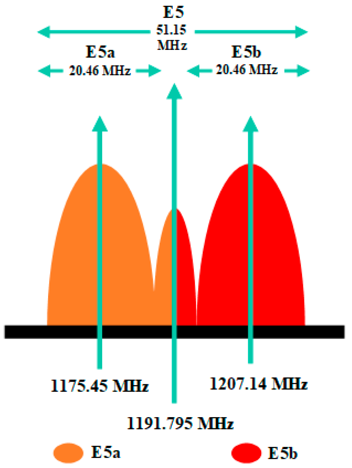
| E5a signal bandwidth (MHz) | 20.46 |
| E5a signal center frequency (MHz) | 1175.45 |
| E5b signal bandwidth (MHz) | 20.46 |
| E5b signal center frequency (MHz) | 1207.14 |
| Receiver bandwidth (MHz) | 100 |
Disclaimer/Publisher’s Note: The statements, opinions and data contained in all publications are solely those of the individual author(s) and contributor(s) and not of MDPI and/or the editor(s). MDPI and/or the editor(s) disclaim responsibility for any injury to people or property resulting from any ideas, methods, instructions or products referred to in the content. |
© 2023 by the authors. Licensee MDPI, Basel, Switzerland. This article is an open access article distributed under the terms and conditions of the Creative Commons Attribution (CC BY) license (https://creativecommons.org/licenses/by/4.0/).
Share and Cite
Cui, Z.; Zheng, W.; Wu, F.; Li, X.; Xu, K.; Ma, X.; Shi, J.; Tao, X.; Zhu, C.; Zhang, X. Improving the Pulse-Limited Footprint Resolution of GNSS-R Based on the Novel Joint Bandwidth Method. Remote Sens. 2023, 15, 4118. https://doi.org/10.3390/rs15174118
Cui Z, Zheng W, Wu F, Li X, Xu K, Ma X, Shi J, Tao X, Zhu C, Zhang X. Improving the Pulse-Limited Footprint Resolution of GNSS-R Based on the Novel Joint Bandwidth Method. Remote Sensing. 2023; 15(17):4118. https://doi.org/10.3390/rs15174118
Chicago/Turabian StyleCui, Zhen, Wei Zheng, Fan Wu, Xiaoping Li, Keke Xu, Xiaofei Ma, Jinwen Shi, Xiao Tao, Cheng Zhu, and Xingang Zhang. 2023. "Improving the Pulse-Limited Footprint Resolution of GNSS-R Based on the Novel Joint Bandwidth Method" Remote Sensing 15, no. 17: 4118. https://doi.org/10.3390/rs15174118
APA StyleCui, Z., Zheng, W., Wu, F., Li, X., Xu, K., Ma, X., Shi, J., Tao, X., Zhu, C., & Zhang, X. (2023). Improving the Pulse-Limited Footprint Resolution of GNSS-R Based on the Novel Joint Bandwidth Method. Remote Sensing, 15(17), 4118. https://doi.org/10.3390/rs15174118