Abstract
Hyperspectral sensors capture and compute spectral reflectance of objects over many wavelength bands, resulting in a high-dimensional space with enough information to differentiate between spectrally similar objects. Due to the curse of dimensionality, high spectral dimensionality can also be difficult to handle and analyse, demanding complex processing and the use of advanced analytical techniques. Moreover, when hyperspectral measurements are taken at different temporal frequencies, separation is likely to improve; however, additional complexities in modelling time variability concurrently with this high spectral dimensionality may be created. As a result, the applicability of ensemble-based techniques suitable for high-dimensional data is examined in this research, together with the statistical evaluation of time-induced variability, since spectral measurements of tree species were taken at different time periods. Classification errors for the stochastic gradient boosting (SGB) and random forest (RF) methods ranged between 5.6% and 13.5%, respectively. Differences in classification accuracy or errors were also accounted for in the assessment of the models, with up to 46% of variation in classification error due to the effect of time in the RF model, indicating that measurement time is important in improving discrimination between tree species. This is because optical leaf characteristics can vary during the course of the year due to seasonal effects, health status, or the developmental stage of a tree. Different spectral properties (assumed from relevant wavelength bands) were found to be key factors impacting the models’ discrimination performance at various measurement times.
1. Introduction
The use of various technologies to gather huge amounts of high-dimensional data has developed and become increasingly important in order to better understand a variety of activities, including strategic and managerial efforts for successful environmental sustainability. Remote sensing technology has long been used to collect data that may be used to map, categorise, and monitor the landscape (ecological and man-made infrastructure), as well as to help in effective planning. Some of these endeavours have often relied on high-resolution spectral and temporal data collected using remote sensing, and/or field or laboratory measurements. Rapid technological innovations in the acquisition of spectral data have resulted in improvements in the description of landscape characteristics, particularly when employing high-resolution satellite imagery [1,2]. Among these applications are the detailed monitoring of ecological ecosystems that require differentiation of vegetation types or communities, detection of plant stress, and mapping of the biochemical composition in vegetative material. The intensive monitoring of ecological ecosystems also involves the detection of plant stress and estimation of the biochemical composition of vegetation material. A wide range of field and/or laboratory instruments, including hyperspectral field spectrometers, Analytical Spectral Devices (ASD), measure reflectance across the major parts of the electromagnetic spectrum (EMS), including visible (VIS), near-infrared (NIR), and short-wave infrared (SWIR). Sparsity is widespread in high-dimensional variable domains because it is impractical to acquire adequate sample sizes. In this work, the use of ensemble classification algorithms based on random forests and gradient-boosting machines is investigated to identify between tree species based on temporal-hyperspectral data. Hyperspectral measurements suffer from the curse of dimensionality, since they collect reflectance over hundreds of tiny bands to form a continuous spectrum. Reflectance is collected and produced in bands (variables) for each recorded leaf measurement, making collecting a large enough sample size to adjust for such dimensionality extremely difficult and costly. When p exceeds n (as is the case here), the available data becomes sparse, and most classifiers, particularly those in the classical statistics domain, become inefficient and sometimes fail to perform mathematical calculations and explore a large search space in the high-dimensional model [3]. There are various classifiers that can handle high-dimensional search spaces for classification and discriminant analysis, including kernel-based approaches such as Support Vector Machine (SVM), ensemble methods such as random forests, boosting models and neural networks. These techniques offer tools for modeling and analysing complex data sets and are largely based on supervised and unsupervised learning and prediction modelling [4].
We use ensemble classification algorithms to distinguish different tree species using high-dimensional hyperspectral data (with highly correlated bands at certain portions of the EMS) with a temporal dimension. Ensemble learning approaches employ a variety of classification techniques, including (1) fundamental learning methods such as decision trees; (2) bagging, which involves averaging and entirety of decision trees; (3) randomisation, which includes bootstrap resampling of observations and variables; (4) sequential development of decision trees, also known as boosting [5]. These techniques are notable for their ability to discover relevant features even in the presence of noise and are useful when dealing with high-dimensional spaces. They are also effective in situations involving small sample sizes, nonlinear relationships between features and responses, and complex interactions between features and responses [6]. As a result, they have been applied in fields as diverse as bioinformatics, cheminformatics and ecology [7]. Furthermore, these methods, particularly random forests, have been applied to regression and classification problems involving large amounts of data in fields such as medicine, agriculture, remote sensing [8], astronomy, finance, online learning and text mining [9,10,11,12]. Ensemble approaches, such as random forest and gradient boosting, combine several techniques using statistical and machine learning frameworks to increase the performance of regression or classification models.
It can be difficult to distinguish or categorise spectrally similar objects measured at a single point in time, especially if these objects (e.g., plants) exhibit changes over time. Dynamic spectral characteristics of objects such as trees may be useful in enhancing the separability of individual trees depending on environmental influences such as seasonal fluctuations in weather or climatic conditions. To improve tree species separation, we used time-induced variations in tree leaf spectra. We are particularly interested in the use of ensemble learning algorithms to characterise tree leaves measured using hyperspectral sensors (which record reflectance over hundreds of variables) at different times (covering different growing seasons). Although we assume that the detailed information in the temporal-spectral measurements will be useful in detecting any small variations that could be used to differentiate between tree species, the high-dimensional search space provided by these measurements presents challenges that should be explored, particularly from the perspective of statistical learning. As a result, a number of research problems arise in this work from both statistical methods and ecological and remote sensing concerns. Statistical issues include whether temporal spectral signatures influence the separation of relevant tree species (i.e., how prediction and validation accuracies vary and if such variations have statistical significance) and identifying spectral signatures (or parts of the electromagnetic spectrum) influencing the separability thereof. From a technological (sensor) application perspective, it is important to determine which of the measurement times provides the best discrimination.
In summary, the purpose of this study is to (1) identify the optimal period for distinguishing tree species, (2) improve species separation by leveraging the effect of measuring trees at different periods, and (3) determine the major drivers (parts of the EMS or spectral wavebands) influencing changes and discriminability of the relevant trees. As a result, we hypothesise that incorporating time-related changes may enhance the discrimination between similar objects, and we anticipate variation in classification errors over time periods.
2. Related Work
Previous research was carried out in the Kruger National Park, which is located in the north-eastern region of South Africa and is characterised by a savannah landscape with an abundant diversity of natural plants and wildlife, supporting a thriving tourist industry in the area. These investigations focused on characterizing dominant tree species using remote sensing technologies (satellite images and field spectroscopy) in order to develop rapid, efficient, and cost-effective strategies for the management of the park. These studies focused on characterizing dominant tree species using remote sensing technologies (satellite images and field spectroscopy) in order to develop rapid, efficient, and cost-effective strategies for the management of the park. This prompted the need for spectrally identifying between predominant tree species and assessing diversity in the park, which proved difficult due to a lack of separation between major species. In situ sensors (spectroradiometers) were then used to capture leaf optical spectra of the main species to create spectral libraries and determine the degree of similarity between savannah tree species [13,14]. These studies discovered greater similarities between some of the tree species, indicating potential difficulties in discriminating between them.
Meanwhile, research questions concerning variability in leaf optical characteristics as a result of phenological interference arose, particularly with a view towards enhancing species separability. Naidoo et al. [15] improved the savannah tree categorisation by integrating multiple technologies such as hyperspectral sensors and LiDAR. This study is thus related to the evaluation of tree separability by studying temporal changes to investigate prospects for enhanced separability amongst trees found in a grassland biome. This biome also contains invasive tree species, the management of which would be efficient if these trees could be easily identifiable through remote sensing. In addition, research by [16] used leaf spectroscopy to compare the separability of Mediterranean tree canopies in two different seasons, demonstrating that changes in canopy profiles helped in better discrimination between relevant trees in one of the seasons. A study conducted by [17] assessed mangrove trees species for seasonal changes in biochemical profiles and phenological phases for species classification in South Africa.
Because of the high dimensionality of the hyperspectral readings, previous investigations derived indicators of optical leaf attributes to evaluate categorisation across seasons or analysed the discriminatory potential of specific bands from different regions of the EMS. In this first part of the study, we utilise all bands to assess separability at various measurement times; hence, we apply the most suitable ensemble learning techniques. It is important to note that this study only examines leaf optical changes during a single growing season and compares the degree of species discriminating across various time periods and seasons.
3. Materials and Methods
Before discussing other aspects of the methodology used, as well as the details about the study area, an overview of the data collection process and mechanism for gathering leaf optical measurements is provided in Figure 1.

Figure 1.
Summary of the data collection process.
The data collection process began with deciding which species to include in the research and selecting those with broad leaves because their reflectance could be readily recorded using the leaf clip of the spectroradiometer, the ASD FieldSpec 4. These reflectance measurements were typically collected every two weeks for a maximum of 21 time periods of measurement.
3.1. Instrument for Data Collection
A portable spectroradiometer, known as the Analytical Spectral Device (ASD) FieldSpec 3, was used to gather leaf reflectance measurements of the target tree species. The ASD is a widely used device in remote sensing applications for ground truthing and examining spectral features of diverse materials such as vegetation, soils, rocks, minerals, and man-made objects. This spectrometer covers a full spectral range between 350 nm and 2500 nm and has a 1.4 nm sampling ratio between a 350 nm and 1050 nm wavelength interval, and a ±2 nm between 1050 nm and 2500 nm regions of the electromagnetic spectrum. The information collected over this full range (Ultraviolet-Visible-Near infrared-Shortwave infrared) is processed and computed for each wavelength band to form hundreds of continuous adjacent signatures. This results in a high-spectral-dimensional space that is considered useful for the analysis of relevant materials.
Since the purpose of this study is to understand how far the seasonal changes (those associated with weather and climate in particular) can be attributed to variability in the leaves of various tree species; which in turn can help to distinguish them spectrally. Therefore, leaf measurements were collected over frequent time intervals (approximately 2 weekly intervals) using the ASD. These tree leaf measurements were gathered using an ASD leaf clip with a built-in plant probe, attached to the spectrometer to simplify the direct and contact measurement of target (e.g., tree leaves and heat-sensitive) objects. The leaf clip collects spectra without interference from the environment and/or external light, therefore eliminating other sources of variability other than those of interest. This is useful since we would like to specifically understand the changes in leaf characteristics without taking into account the other sources of variability affecting the spectral signature of the leaves, which include the tree canopy and background material. Instead, we focus on the mechanism of change in the physiological properties of leaves, driven by seasonal effects.
3.2. Study Location and Data Collection Process
As indicated, this study makes use of the hyperspectral leaf measurements as a primary data set used in order to separate spectrally similar tree species gathered at close time intervals. With a spectro-temporal database of the common seven indigenous tree species and common invasive weed in the Highveld grassland biome, their leaf measurements were collected from June 2011 until May 2012. The data collection site is located in the eastern part of Pretoria at the Council for Scientific and Industrial Research, City of Tshwane, Gauteng Province, South Africa. While this study site is an urbanised environment, it is known to be one of the few remaining parts of the original bushveld [18], as it predominantly contains indigenous vegetation and some wildlife that has been conserved for decades. This site is known to be one of the representative locations for the city’s surviving natural grassland and savanna vegetation, while the city is well-known for the abundance of Jacaranda mimosifoliatrees, which are considered invasive plants in South Africa.
3.2.1. Selection of Tree Species
Prior to conducting fieldwork, a walk-through inspection was performed to identify the common tree species at the study site. Eleven tree species were found to be predominant in the study area, including an alien invasive weed known as the lantana camara. Eight out of the eleven species were identified as the primary sampling units in the sampling frame. The excluded trees included Acacia caffra, Euclia crispa and Rhus leptodictya. These were excluded purely for practical reasons because their leaves are too small and require a lot of effort to assemble and clip with an ASD plant probe for measurement.
Table 1 provides a list of the eight tree species included in the study and their classification according to leaf longevity characteristics. This categorisation provides an important source of information with respect to temporal vegetation spectroscopy and terrestrial remote sensing, as deciduous trees lose all their leaves seasonally while evergreens do not. As a result, the total number of samples varies in size, leading to some imbalance at the category level.

Table 1.
Names of the 8 tree species measured and their leaf-response characteristics.
3.2.2. Leaf Sampling, Collection of Leaf Reflectance Measurements and Storage
The process of sampling the trees was conducted as follows: five different trees from each of the eight species were chosen for leaf sampling; they were marked with a red tape and their GPS locations were recorded. In total, 40 trees were selected and measured at two-week intervals throughout the annual growth cycle. However, there were gaps in data collection due to practical constraints, including the unavailability of the ASD and when deciduous trees had lost all their leaves. As a result, deciduous trees including Celtis africana, Combretum molle and lantana camara exhibited missing observations at the time when the leaves had lost all their leaves. The resulting temporal-hyperspectral database of the tree–leaf reflectance measurements was made up of 21 measurement periods (weeks), with specific dates recorded throughout the data collection period.
Having concluded the selection of trees from which the leaves would be measured using the ASD, a leaf sampling procedure was developed and followed throughout the data collection period. This involved selecting seven leaves from each tree to represent the current state of a tree crown. In order to reduce random noise or measurement variation within species, the leaves were selected from the tree crown to represent the canopy and allow any prospective comparison with a satellite image. In addition, the samples were scanned with white referencing conducted in-between measurements, so as to ensure the adequate calibration of the instrument.
In order to facilitate speedy collection and measurement of the leaves during fieldwork and avoid carrying a bulky spectrometer into the site, leaves were collected, placed in marked plastic bags and stored in the cooler box (containing a few ice bricks) in order to reduce transpiration which results in dehydration of leaves as well as induced changes in leaf spectra. Labelling on plastic bags, which identified the name (abbreviated) of tree species and the number assigned to a specific tree, was made prior to the start of fieldwork. The numbering of trees of the same species followed the same pattern as that on the red-tapped trees, to avoid any possible mix-up of leaf samples. The stored leaves were then taken into the laboratory (dark room) for measurement with an ASD leaf clip and probe. The ASD technical guidelines [19] were studied and followed when taking the measurements. Assistance was provided by the colleagues who owned and housed the instrument, including providing a complete demonstration process of using the machine, including the assembly, set up, gathering of leaf reflectance measurements, and storage of the data. The guidelines that followed involved setting and warming up the instrument for at least 30 min prior to collecting measurements. Furthermore, the instrument had been calibrated after each batch (a plastic bag containing leaves from one tree) of tree leaf samples were measured for reflectance. Each recorded batch was named using the abbreviated names of the tree species and the number marked in the plastic bag. Renaming each batch of measurements was conducted along with the calibration intervals.
3.2.3. Processing of Leaf Measurements
Multiple files containing stored leaf profiles gathered at specific time periods were imported into Statistical Analysis Systems (SAS) software for pre-processing and management. This step included reformatting the data structure and inputting additional identifiers (full and abbreviated names of tree species, full date formats, weeks, months and seasons) for each of the observations (tree leaf samples).
At the end of the fieldwork, a total of about 5220 leaf reflectance samples had been collected over 21 measurement periods or times, from the 8 classes of tree species shown in Table 1. Since deciduous trees lost leaves during the winter months, the total number of leaf samples varied between 182 and 280 during different measurement periods.
3.3. Data Analysis Techniques
This study explores the implementation of ensemble classification methods involving random forests and gradient boosting machines to distinguish between tree species from temporal-hyperspectral measurements. Since hyperspectral measurements collect reflectance over hundreds of narrow bands which form a continuous spectrum, these measurements suffer from a phenomenon known as the curse of dimensionality. For each leaf measurement taken, reflectance is collected and produced at p = 2100 bands (variables), making it extremely difficult and costly to collect a large enough sample size to compensate for such dimensionality. When p is too large and even exceeds n (as is the case here), the available data become sparse; most classifiers, particularly those in the classical statistics domain, become inefficient and sometimes fail to perform mathematical computations and explore a large search space in the high-dimensional model [3]. There are several classifiers, for instance, that can handle high-dimensional search spaces for classification and discriminant analysis, and they include kernel-based methods such as support vector machines, ensemble methods including random forests and boosting models, and the neural networks. In this study, we adopt the ensemble classification methods to discriminate between tree species from high-dimensional hyperspectral data (with highly correlated bands at specific parts of the EMS) involving a time dimension. These methods are known to have the ability to detect relevant features even in noisy environments and are convenient when dealing with high-dimensional feature spaces. Moreover, they are useful in situations where small sample sizes are collected, and non-linear and complex relationships between the feature and the response exist [6]. As a result, they have been applied in areas including bioinformatics, chemoinformatics, and ecology [7]. Moreover, the application of these methods, particularly random forests, has been used for both regression and classification problems involving large amounts of data across fields such as medicine, agriculture, remote sensing [8], astronomy, finance, online learning, and text mining [9,10,11,12]. In this paper, we focus on the application of the tree-based ensemble involving random forest and gradient boosting. Random forest and gradient boosting methods are known as ensemble techniques since they use multiple techniques involving statistical and machine learning principles in order to improve the performance of regression or classification models.
3.3.1. Random Forest
In classification, the random forest is an ensemble classifier that has gained popularity in statistical and machine learning applications. RF constructs multiple decision trees by employing a combination of methods including bootstrap re-sampling, decision trees and bagging. Random forests create an ensemble of decision trees that are grown by randomly generating a bootstrap sample of observations and a random set of variables (spectral bands), letting them vote for the most popular class via the bagging technique [6]. Random forest operates by randomly selecting a subset of variables from a training data set, building decision trees for each bootstrap sample by continually splitting trees and growing them until the forest is as large as desired. The predictions from all decision trees are then combined to generate the final prediction, in which the majority class is selected. To minimise overfitting during the training phase, the random forest’s performance may be evaluated using a test set. Random forest selection bias pitfalls need to be remembered, particularly when it comes to identifying features that discriminate between classes, where important variables may be omitted, with their significance being ignored or underestimated. For this reason, more robust variable selection techniques for the random forest model were considered. Some of these methods are based on regularised random forest estimation which employs a sequential forward selection process while assessing information gain [20]. Others are based on permutation testing using holdout approaches for importance measures [21], whilst others are based on Conditional Inference Forest [22] or by employing mechanisms to prevent overfitting [23]. Conditional inference-based approaches [22] were used in this study to minimise bias in the selection of important features while evaluating the significance of the correlations between the predictors and the response variable (category).
3.3.2. Gradient Boosting
Gradient boosting methods also make use of various techniques to reduce bias and improve predictions. Just like random forest, GBM is an ensemble classifier which uses re-sampling techniques, decision trees and bagging but additionally makes use of a technique known as a gradient descent in minimizing the classification error, otherwise referred to as a loss function. In the boosting framework, initial decision trees are computed from a random sample of observations from the data set. After the trees are evaluated for their classification potential, subsequent trees are constructed based on the information from the previous trees. This information involves evaluating observations that were difficult to classify and giving them more weight while decreasing the weight of easy-to-classify observations [24]. Therefore, a second set of trees is grown on weighted data in order to improve the prediction of the previous set of trees; a common method for this is known as adaptive boosting [6,25]. This process is repeated until a desirable number of trees have grown from several iterations. In this study, the stochastic gradient boosting technique was applied to minimise the error associated with classifying observations into true classes rather than a wrong class. Stochastic gradient boosting is different from the normal gradient boosting technique in that it randomises the computation of the average loss by calculating it from a randomly selected (without replacement) fraction of the training data set. This randomisation process is implemented to improve performance by reducing the degree of correlation between trees and to avoid a model overfit [26]. Stochastic gradient boosting is regularised by a training parameter known as the learning rate.
3.3.3. Evaluation of the Model Performance
A variety of metrics are used in classification problems to measure the effectiveness of a classifier in accurately differentiating between sets of observations. To minimise model overfitting, the provided assessment metrics were derived using test data sets comprising around 33% of the observations from each measurement period, whereas training data sets containing roughly two-thirds of the observations were used to build the models. In this study, we apply a number of these evaluation indicators, focusing primarily on tracking classification errors over time in order to investigate whether changes in leaf spectral properties have a statistically significant temporal pattern. As a result, the majority of the findings are analysed in terms of classification errors, although overall accuracy, kappa, and area under the Receiver Operating Characteristics (ROC) curve (AUC) are also used to summarise the performance of the classification models throughout different measurement periods. The overall accuracy is defined as the fraction of correctly classified predictions, or the proportion of true positives and true negatives in the sample. One of the summary statistics used to evaluate the performance of a classification technique is the AUC, which measures the level of discrimination between two or more categories, was also considered. Even though values in the probability space might vary from 0 to 1, AUC is interpreted using a probability threshold value of 0.5. When AUC is 0.5, the model has no statistical ability to distinguish between classes, whereas AUC values less than 0.5 and near zero suggest that the model predicts a negative class as a positive class, and the other way around. AUC of 1 indicates that the model accurately differentiates between the relevant categories. To evaluate the overall performance of the model, micro AUC was calculated to compute the area under the curve for multiple classes, as shown in the findings. The Kappa statistic is another evaluation metric that may be used to examine the model’s capacity to discriminate between groups, with values ranging from 0 to 1. The Kappa statistic, which ranges from 0 to 1, is another assessment measure that may be used to assess the model’s ability to differentiate across groups. Kappa values near 0 suggest that categorisation is insufficient, whereas a value of one indicates perfect separation between classes.
3.3.4. Feature Selection
Determining the variables that are important in the prediction of true classes is an essential part of any classification problem, and the two models investigated in this work offer such capabilities. In this application, understanding the key variables is of the utmost importance because this identifies the primary spectral characteristics that drive variability through time, enhancing species separability at different times in the growing season. It is also of interest in this study to determine how seasonal or temporal variations impact both the biophysical and biochemical components of the leaves by examining spectral features that discriminate between the relevant tree species at various measurement times.
It is important to note that the application of the classification algorithms was re-adjusted to achieve the best results. Classical random forest models, for example, employ randomness to reduce the correlation among trees, but this can lead to feature selection bias because variables with more potential splits may be favored. For this reason, a more robust method was used to reduce bias in the selection of the spectral signatures with better predictive contribution, especially in the random forest. A conditional inference-based approach [22] was used in this study to minimise the bias in the selection of important features while evaluating the significance of the correlations between the predictors and the response variable (category).
4. Results
The results of the classification derived from RF and GBM models, including prediction errors and important variables for species discrimination at each measurement time, are presented in this section. The average classification errors generated from these models across the measurement periods (Time 1 through to 21, covering different seasons) are shown in Figure 2, with the 95% confidence bands as measures of uncertainty associated with these errors. In terms of the findings from RF, this model provided an average out-of-bag error of roughly 13.5%, with time-specific average errors ranging from 1.4% to 32%, indicating changing patterns in leaf properties during the interannual growing season of the relevant tree species.
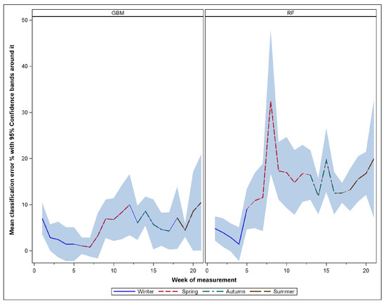
Figure 2.
Classification error variation by measurement period and season for each model.
Further detail provided in the right-hand panel of Figure 2 generally illustrates an increasing pattern of classification inaccuracies from winter through to autumn, with some fluctuations within and between seasons. It is also noticeable from this figure that the measurements gathered during the winter month (from June to August) produced relatively lower classification errors (ranging from approximately 1.4% to 9%) compared to other seasons. The highest classification inaccuracies (exceeding 30% error rate) were obtained from one of the measurements collected during one of the spring months (specifically Time 8, on the 28th day of September), with the highest possible error almost reaching 50% as per the upper confidence limit.
Regarding the results of GBM, the classification inaccuracies were generally lower (average classification error of 5.6%) than those of the random forest model. At a detailed level, the average error classification at each of the measurement times ranged from a minimum average error of about 0.8% observed from the beginning of the spring season to the largest classification error of about 10.5% observed from measurements gathered in autumn. However, the temporal pattern of the GBM classification errors was not as variable as that of the RF errors since larger error fluctuations were more pronounced in the random forest models.
Having observed temporal variability in the pattern of classification errors resulting from both models, it was important to examine whether there is enough statistical evidence to suggest that the average difference in classification errors is due to differences in the times at which these hyperspectral leaf measurements were gathered. In addition, we quantified the amount of variation that time accounts for in explaining the observed variations.
A statistical analysis was conducted in which a generalised linear model was used to determine whether the average classification error for the measurement time varied significantly. To determine whether there were significant changes in the mean error, specifically over time, we used the least squares difference (LSD) at an alpha () level of . The model suggested that at least one of the time points is statistically different with respect to classification errors obtained from the random forest model and that the measurement time accounts for approximately 46% of the variation in these errors. A multiple comparison of the effect of time on classification errors is shown in Figure 3, with distinct pairs of time shown by blue diagonal lines, while those that are not statistically different are indicated by red diagonal lines. In this figure, the mean classification error for time is shown along the x-axis, with the mean error of the other time along the y-axis with a dot at the intersection. The identity line represents the equality of means such that if a vector does not cross this line, we can conclude that the means’ mean errors are significantly different between relevant time periods. Otherwise, the means are similar if the lines cross the identity line. Red vectors are used to identify significant differences between time periods, whereas blue lines indicate time vectors with similar classification errors with respect to their average errors. It is most noticeable in Figure 3 that most error differences occurred between Time 8 (with the largest mean error of about 32% and representing a measurement period in September) and the rest of the other measurement periods. Other pairs of time where distinct differences occur mostly include time pairs that are farther apart. For example, the earlier time periods that included measurements gathered between June and July consistently differ (in terms of average classification inaccuracies) from the later measurements taken in January and May of the following year. Regarding understanding the variation of errors from the boosted model, the analysis indicates that measurement time has an effect on the variation of classification errors and accounts for nearly 21% of these differences. Generally, differences in the temporal pattern of these errors are not as pronounced as differences obtained from the random forest model.
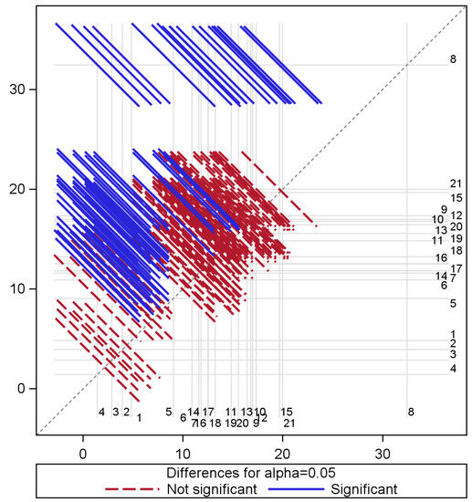
Figure 3.
Multiple comparisons of random forest class prediction error means for time.
Figure 4 shows pairs of time periods that are statistically different with respect to their average prediction errors. From this model, the mean error from Time 21 (from end-of-May measurements) significantly differs from the earlier measurements (taken from the start of data collection in June to the end of September, as well as in February and March). Time 12 errors representing classification errors from measurements gathered towards the end of November are also distinct from the average errors of measurements gathered from June through to the end of September. Therefore, the variation of errors in time is more evident from the random forest model as compared to the GBM model.
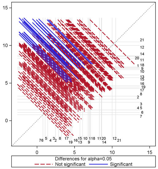
Figure 4.
Multiple comparisons of GBM class prediction error means for time.
Figure 5 provides a graphical view of classification inaccuracy patterns from the random forest model at various measurement time periods, for each of the eight species. The plotted points represent the time interval values at which the spectral reflectance of each species was gathered across the distribution range of class prediction errors to highlight the time periods that influence classification inaccuracies. These results generally show that discrimination between species is not constant in time and that some species appear to be more accurately distinguishable at different times than others.
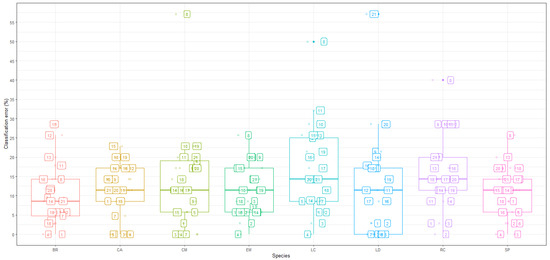
Figure 5.
Random forest: Classification errors of species at specific time points.
Tree species that appeared to be easily separated via the random forest model include Celtis africana, Englerophytum magalis, Brachylaena rotundata, and Strychnos pungens as their classification inaccuracies were largely below 30%. Meanwhile, species such as Combretum molle and Lannea discolour had at least one time point in which their classification rate was no better than the random allocation (classification errors exceeding 50% and the highest reaching 57%) for both CM and LD at time 8 (30 September) and 21 (25 May), respectively.
The smallest classification inaccuracies occurred in the June to August measurements for all tree species. The pattern of inaccuracies observed at a species level corresponds to the generic patterns discussed above. However, additional information suggested that even though the highest average classification error came from the random forest model, species-level classification errors were subject to larger variations in classification rates. The influence of these larger errors, with seemingly outlier properties, had an influence on the average errors in Figure 2, particularly for Time 8, which stands out as having the largest inaccuracies.
Species-level classification inaccuracies from the GBM model are shown in Figure 6, and the variation of these errors is not very different from that of the random forest model, even though there is a slight reduction in the magnitude of errors obtained from GBM. Similar species that were highlighted as having the largest classification errors at certain time periods, by the random forest model, maintained that pattern from the GBM results as well. The major difference, however, is that the measurement periods that generate larger errors (those greater than 20%) from GBM are different. This is with the exception of Time 21, which appears in both models as one of the highest error time periods where species such as LD and RC were not easily distinguishable. Another difference, for instance, is that larger errors from GBM were associated with clusters of times including periods in May (times 20 and 21), April (Time 18) and November (Time 11 and 12). Another important element of classification involves performing a diagnostic assessment of the model performance by summarising the resulting confusion matrix (matrices) rather than observing the accuracy or error rate on a generic scale.
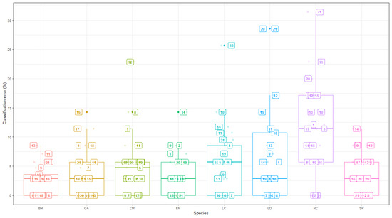
Figure 6.
GBM: Species classification errors at specific time points.
Figure 7 compares the classifiers’ performance based on the micro AUC, demonstrating that both models provided an adequate categorisation of the tree species, with GBM offering a slightly superior discriminatory ability than RF for a majority of the periods in question. The pattern of variability in accuracy through time appears to be consistent with the insights which have already been revealed in preceding results.
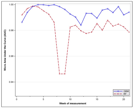
Figure 7.
Model evaluation: Micro AUC variation by time of measurement.
Table 2 provides a summary of the model accuracy statistics including accuracies and their confidence limits (CI) as well as the Kappa coefficient. The Kappa coefficient is sometimes viewed as a more robust measure since it also accounts for the likelihood of agreement between a true and predicted classification of categories by mere chance. As can be observed from Table 2, the values of kappa are slightly lower than those of accuracies because kappa penalises the statistic by incorporating random chance as compared to a percentage measure. Since there are no agreed-upon threshold values for levels of agreement, different areas of research assign various thresholds to indicate poor, good, or exceptional discrimination between objects. The findings indicate that accuracy in categorizing tree species varies over time, demonstrating that time could influence the level of discrimination between trees because of the changes in spectral properties through time.

Table 2.
Model accuracy with 95% confidence intervals and Kappa values for each measurement period.
Time periods with relatively lower classification accuracies and kappa values are highlighted in yellow and blue in Table 2 to highlight those times when the models achieved moderate classification performance. The confidence intervals for overall accuracies also show the degree of uncertainty surrounding the classification, with certain time periods having wider confidence limits, suggesting more fluctuation around the values.
Figure 8 presents important variables in the prediction of the eight species for the initial measurement periods (winter months) with the top 25 variables (wavelength bands denoted by a prescript ’B’) identified using an unbiased feature selection for the random forest. Time 1, which corresponds to the time period (10 June) when measurements of the relevant species’ leaf reflectance properties were first collected, reveals that the most relevant spectral signatures for species discrimination were largely from the NIR part of the electromagnetic spectrum, with some of the few red-edge position bands located between 670 nm and 780 nm which are closely associated with the pigment status and physical and chemical properties of vegetation [27]. Time 2 consists of bands from similar regions as Time 1 but also contains a few more signatures from the VIS region, 401 nm and 669 nm. The VIS bands are known to have strong chlorophyll absorption and are sensitive to photosynthetic pigments and characteristics including biochemicals such as carotenoids (responsible for the orange pigment), chlorophyll (green pigment) and xanthophyll (yellow pigment).
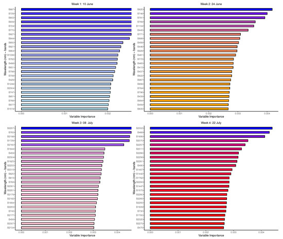
Figure 8.
Random forest: Important variables (reflectance bands) for tree species discrimination, per measurement time.
The classification of species in Time 3 seems to be driven largely by the bands from the SWIR part of the spectrum which generally provide information about leaf structure, proteins and nutrients, whereas Time 4 shows a somewhat different profile of signatures which played a significant role in the discrimination of species.
The classification of species in Time 3 appears to be largely driven by bands from the SWIR part of the spectrum, and these bands typically provide information about leaf structure, proteins, and nutrients. Time 4, meanwhile, shows a slightly different profile of signatures that played a significant role in species discrimination. Additional graphs are provided in the Appendix A and Appendix B, demonstrating the changing spectral attributes which may be useful in the characterisation of tree species based on leaf properties or temporal condition.
Figure 9 depicts the bands identified as the most important by the GBM model in relevant winter weeks. Regarding Time 1, GBM mostly selected the signatures from the NIR range of the EMS, especially those in the red-edge region, and very few SWIR signatures, as the most important bands in discriminating between species. For Time 2, the strongest signatures identified by GBM were predominantly those from the VIS (with mainly blue, a few red, and green bands), NIR and the SWIR regions. Time 3 had a number of SWIR bands, a mix of red, blue, and green bands from VIS, and only one NIR signature, just as in the previous two time points. The important bands in separating species from Time 4 include those from SWIR, VIS (with no yellow bands included), and a few NIR bands.
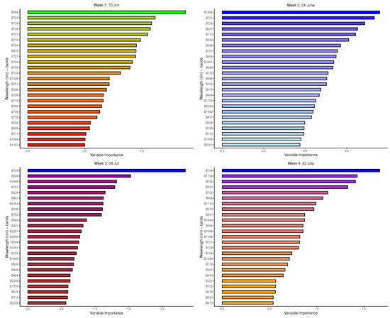
Figure 9.
GBM: Important variables (reflectance bands) in the prediction of the 8-class tree species.
It is important to note from the analysis of important variables that, while the random forest and GBM produced somewhat different lists of variables at various measurement times, these models did identify these variables largely from the same regions of the EMS. In general, this analysis shows that different wavelength bands from various regions of the electromagnetic spectrum contribute differently to the discrimination of the species depending on the time at which the measurements were taken. The main observation from the results is that the different parts of the electromagnetic spectrum can play different roles in the discrimination of trees depending on the time at which these measurements are gathered.
5. Discussion of the Results
This investigation is part of a larger project that aims to improve separability between similar tree species using hyperspectral measurements by incorporating variability in leaf characteristics that occurs over time due to seasonal changes during the annual growing cycle of plants. Because of high spectral dimensionality, ensemble learning techniques involving random forest and GBM were used in distinguishing between tree species at different times. Second, it was important, from an ecological perspective, to identify the time period at which the separability between the relevant tree species (from a leaf-level perspective) could be most favourable. The discussion of the results is anchored around these two main aspects.
5.1. Comparative Assessment of Class Prediction Accuracy between Random Forest and GBM
Previous studies that have compared the prediction accuracy between random forest and gradient boosting methods, particularly in remote sensing applications, have not reached the same conclusions regarding their performance. In the recent review involving the use of random forests in remote sensing [8] the included studies made a comparative assessment of the classification accuracy results between random forests and boosting ensemble techniques such as adaptive boosting and concluded that random forests provided better classification results than boosting ensembles. Meanwhile, specific studies in the same review [8] found that these two sets of methods provided similar classification results, with RF gaining favour due to its stability and less computationally intensive requirements [28,29]. However, in an investigation by [29], however, slightly improved classification results were obtained from specific booting techniques (AdaBoost tree and AdaBoost random) compared to random forest and bagging tree methods. Another recent study by [30], which applied extreme gradient boosting (XgBoost), random forest, and SVM for object-based classification of the relevant types of Land Use-Land Cover (LULC) types, found that XgBoost outperformed random forest and SVM.
From the results obtained in our study, a stochastic gradient boosting technique outperformed the random forest with respect to the accuracy of the classification across time intervals. It is important to note, however, that the random forest was able to account for larger differences between species at various measurement periods. This could be explained by a known phenomenon associated with random forests being sensitive to imbalanced training samples, thus favouring the most represented classes. In our case, class imbalances occurred, particularly because deciduous trees had fewer samples during leaf shedding times. Moreover, it appears that the random forest was more sensitive to intra-species-level variability. For example, the random forest achieved the largest average classification error at measurement time period 8 (consisting of measurements collected at the end of September), where larger errors were generated from (Combretum molle) reflectance measurements with a few newly emerging leaves. Generally, species with fewer measurements tended to have the highest average classification inaccuracies, and errors were obtained from deciduous tree species with lesser measurements at relevant time periods. Therefore, the random forest maximised the degree of differences between measurements collected at different time points, accounting for double the amount of temporal variability compared to the boosted ensemble.
5.2. Important Variables
Although opportunities exist to reduce the high dimension of wavebands from hyperspectral measurements without losing much useful information, high correlations between adjacent bands of these measurements make it challenging to perform the exact band selection. Therefore, the intention for identifying bands with high discriminatory potential was not to directly pinpoint the exact bands, but rather to identify prominent regions of the EMS, as well as to assess their contribution based on known reflectance properties.
Other phenological-based applications that have used phenological analysis to understand periodic patterns of change in vegetation characteristics and the extent to which these are altered by changes in seasonal or climatic variations; mostly based on remote sensing, in situ, and laboratory data to examine such changes. A study by [16] is among a few studies in which phenological events were studied to establish the potential to improve the classification between tree species. Specifically, this study used laboratory measurements gathered from two simulated stages, including flowering and nonflowering stages, and established that the classification between species was enhanced during the flowering stage (measurements gathered in July), with prominent differences from the VIS part of the electromagnetic spectrum. In a study by [31], where leaf properties were examined based on laboratory measurements, the authors discovered that signatures in the visible range explained variations in the relevant properties. Everitt et al. [32] studied the impact of flowering on VIS and NIR spectra of Drummond goldenweed species and found that these species were only distinguishable from others based on VIS bands during the flowering stage. However, during non-flowering, the NIR bands of the goldenweed species were separable from other relevant species. Hence, from these studies we can conclude that even though VIS has a greater influence on the separation at certain times, other regions have a significant contribution depending on the measurement time and prevailing characteristics.
Generally, our study established that leaf phenology variations and the potential to spectrally distinguish target tree species classes were driven by various spectral characteristics at different time periods. Different sets of VIS bands were consistently identified as being some of the important bands in discriminating between tree species, at different times. There was, however, a strong combination of NIR and/or SWIR bands along with the VIS wavebands, which provided a better discriminatory ability. This indicates that photosynthetic characteristics were predominantly driving the prediction of species while SWIR and NIR, which characterise leaf structure, proteins and starches, age, leaf health and nutrients, also played a significant discriminatory role. Since two different models were applied in this study, it is important to note that these models did not always select similar spectral characteristics when looking at the top 25 important variables. It is, however, worth noting that similar sets of bands, especially those in the VIS range, were identified in both models, while most inconsistencies were with respect to the selection of NIR and SWIR wavebands. In the view of the changing spectral properties with time, this study suggests that it may be limiting to use the same set of bands (drivers of separability) for prediction at other times, especially when using band-level information.
5.3. Best Time to Distinguish between Species
Since it can be relatively costly to acquire high resolution satellite imagery, the optimal time for acquiring images has been studied for monitoring and managing ecological applications or agricultural sites with varied imaging technologies. Some of these investigations have been conducted on multiple temporal images to capture the variability across the growing season and to determine the best time for observing and identifying specific characteristics as well as classifying crop types, trees and grass species, as these have changing characteristics over time. Using aerial images, Lisein et al. (2015) [33] were able to determine that spring and fall (end of leaf flushing) were the best times for species separation. Hill et al. (2010) [34] combined temporal images to find that using a combination of 17 March, 16 July, and 27 October had the greatest overall classification accuracy, at 84 percent (green-up and full-leaf phases were optimum). In this study, which used in situ temporal hyperspectral leaf measurements, we discovered that the best time for differentiating tree species was during the winter and spring seasons.
6. Conclusions
This study explored the applicability of ensemble classification methods, including random forest and gradient-boosting machines that use decision trees for base learning, while employing a variety of techniques in attempts to correctly assign observations to their respective groups. Most importantly, this study sought to establish the effect of time on the classification inaccuracies of the target tree species, since their leaf hyperspectral measurements were collected at frequent time intervals. We model temporal spectral characteristics changes that can enhance the separability between these spectrally similar tree species. The gradient boost performance was generally superior to that of the random forest, since GBM produced relatively lower classification inaccuracies (mean classification error of 5.6%) across different measurement periods, while the random forest had an average OOB error of approximately 13.5%. The GBM classification errors did not have a distinct temporal pattern compared to the errors resulting from the random forest model. Classification errors obtained from GBM did not vary greatly and had overlapping distributions across measurement periods, while RF errors showed an increasing pattern from winter measurement periods through to autumn of the following year. Relatively, winter measurements had the lowest class prediction inaccuracies, whereas autumn had an outlying time period where classification errors were the largest. Further analysis of inaccuracies from the random forest model indicated that average classification errors are statistically different, and that time accounted for about 46% of the variation in the mean classification error, while the effect of time accounted for about 21% of the mean error from the gradient boosting technique. The study therefore shows that leaf-level discrimination of tree species can be improved depending on the time of measurement since spectral profiles of trees vary with changing weather conditions.
In terms of the evaluation of important variables, two models were useful in identifying the variables that contribute the most to the separation of relevant tree species at different measurement periods and those with little or no influence on the model. These models produced slightly different sets of important predictor variables at various time periods, while some similarities were observed for other time periods. Here, the idea was not to search for individual variables but to establish whether spectral bands of similar characteristics over the wavelength range were consistently identified as being of high relative importance in both models at similar measurement times. Although variables of high importance varied across measurement periods, indicating changing spectral reflectances due to time conditions, the changes were not similar between models, making it difficult to establish which are the key distinguishing drivers (spectral regions) across time. However, due to the fluctuating nature of optical spectral features over time, predicting band-level categorisation using a selected set of bands across consecutive periods may not yield satisfactory results.
Author Contributions
The authors affirm their contributions to the paper as follows: Study conception and design, N.D.-T., M.A.C. and P.D.; Methodology, N.D.-T., M.A.C. and P.D.; data processing and analysis, N.D.-T.; writing—original draft preparation, N.D.-T.; writing—review and editing, O.M., P.D. and M.A.C. All authors have read and agreed to the published version of the manuscript.
Funding
This research received no external funding and the APC was funded by the Council for Scientific and Industrial Research (CSIR).
Data Availability Statement
The data presented in this study may be obtained from the corresponding author upon request. Due to intellectual property and confidentiality concerns, the data is not publicly available.
Conflicts of Interest
The authors declare no conflict of interest.
Abbreviations
The following abbreviations are used in this manuscript:
| EMS | Electromagnetic Spectrum |
| GBM | Gradient Bossting Machine |
| LSD | Least squares difference |
| LULC | Land-Use Land Cover |
| NIR | Near infra-red |
| OOB | Out-of-bag error estimate |
| RF | Random Forest |
| SVM | Support Vector Machine |
| SWIR | Shortwave infra-red |
| VIS | Visible |
| XGBoost | eXtreme Gradient Boosting |
Appendix A. Important Variables from Random Forest for Measurement Times 5 to 21
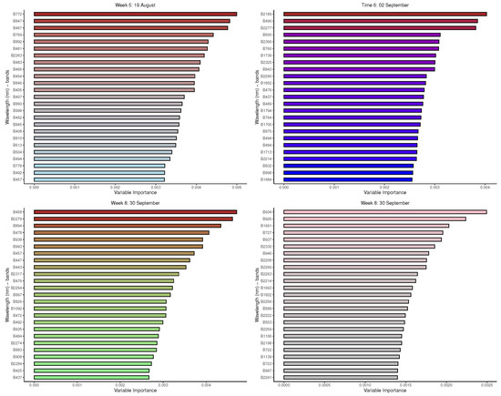
Figure A1.
Random forest: Important variables in predicting 8-class tree species by measurement period: 5 to 8.
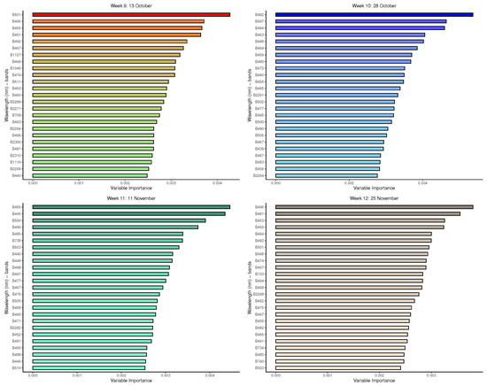
Figure A2.
Random forest: Important variables in predicting 8-class tree species by measurement period: 9 to 12.
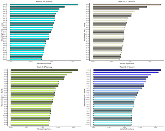
Figure A3.
Random forest: Important variables in predicting 8-class tree species by measurement period: 13 to 16.
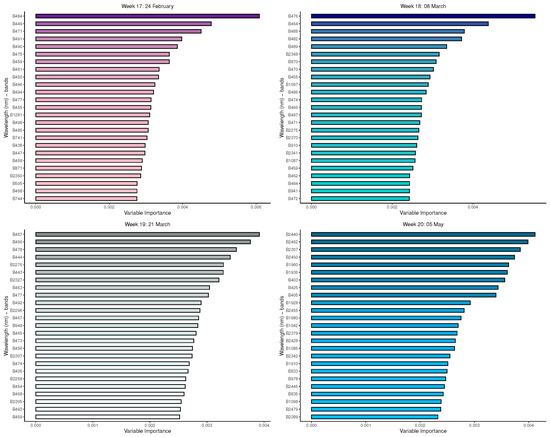
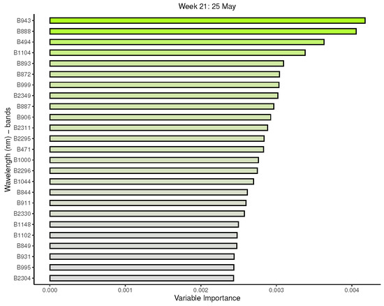
Figure A4.
Random forest: Important variables in predicting 8-class tree species by measurement period: 17 to 21.
Appendix B. Important Variables from GBM for Measurement Times 5 to 21
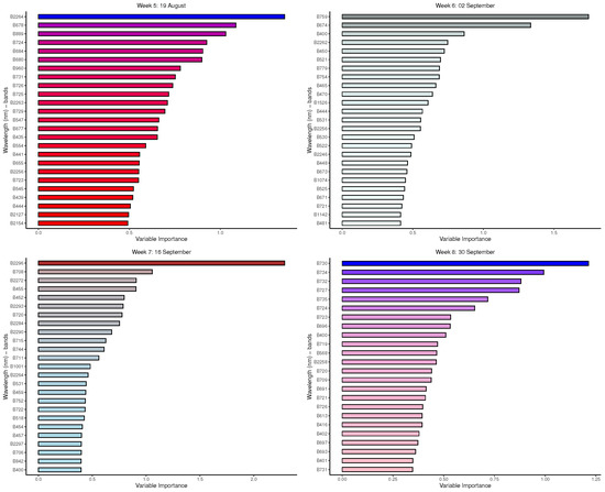
Figure A5.
GBM: Important variables in predicting 8-class tree species by measurement period: 5 to 8.
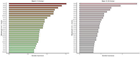
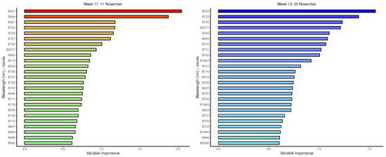
Figure A6.
GBM: Important variables in predicting 8-class tree species by measurement period: 9 to 12.
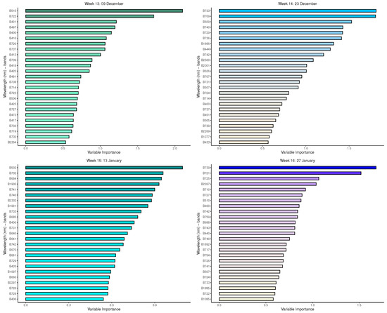
Figure A7.
GBM: Important variables in predicting 8-class tree species by measurement period: 13 to 16.
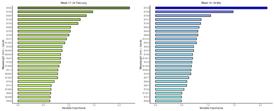
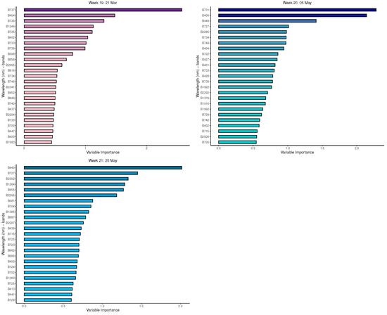
Figure A8.
GBM: Important variables in predicting 8-class tree species by measurement period: 17 to 21.
References
- Mustapha, A.; Aris, A.Z.; Ramli, M.F.; Juahir, H. Temporal aspects of surface water quality variation using robust statistical tools. Sci. World J. 2012, 2012, 294540. [Google Scholar] [CrossRef] [PubMed]
- Mutanga, O.; Van Aardt, J.; Kumar, L. Imaging spectroscopy (hyperspectral remote sensing) in southern Africa: An overview. S. Afr. J. Sci. 2009, 105, 193–198. [Google Scholar] [CrossRef]
- Zou, H. Classification with high dimensional features. Wiley Interdiscip. Rev. Comput. Stat. 2019, 11, e1453. [Google Scholar] [CrossRef]
- James, G.; Witten, D.; Hastie, T.; Tibshirani, R. An Introduction to Statistical Learning; Springer: Berlin/Heidelberg, Germany, 2013; Volume 112. [Google Scholar]
- Dietterich, T.G. An experimental comparison of three methods for constructing ensembles of decision trees: Bagging, boosting, and randomization. Mach. Learn. 2000, 40, 139–157. [Google Scholar] [CrossRef]
- Zhang, C.; Ma, Y. Ensemble Machine Learning: Methods and Applications; Springer: Berlin/Heidelberg, Germany, 2012. [Google Scholar]
- Scornet, E. Tuning parameters in random forests. ESAIM Proc. Surv. 2017, 60, 144–162. [Google Scholar] [CrossRef]
- Belgiu, M.; Drăguţ, L. Random forest in remote sensing: A review of applications and future directions. ISPRS J. Photogramm. Remote Sens. 2016, 114, 24–31. [Google Scholar] [CrossRef]
- Goel, E.; Abhilasha, E. Random forest: A review. Int. J. Adv. Res. Comput. Sci. Softw. Eng. 2017, 7, 251–257. [Google Scholar] [CrossRef]
- Qi, Y. Random forest for bioinformatics. In Ensemble Machine Learning; Springer: Berlin/Heidelberg, Germany, 2012; pp. 307–323. [Google Scholar]
- Genuer, R.; Poggi, J.M.; Tuleau-Malot, C.; Villa-Vialaneix, N. Random forests for big data. Big Data Res. 2017, 9, 28–46. [Google Scholar] [CrossRef]
- Cutler, D.R.; Edwards, T.C., Jr.; Beard, K.H.; Cutler, A.; Hess, K.T.; Gibson, J.; Lawler, J.J. Random forests for classification in ecology. Ecology 2007, 88, 2783–2792. [Google Scholar] [CrossRef]
- Majeke, B.; Cho, M.A.; Debba, P.; Mathieu, R.S.; Ramoelo, A. Species Discrimination of African Savannah Trees at Leaf Level Using Hyperspectral Remote Sensing. 2009. Available online: https://researchspace.csir.co.za/dspace/handle/10204/3291 (accessed on 7 August 2023).
- Dudeni, N.; Debba, P.; Cho, M.; Mathieu, R. Spectral band discrimination for species observed from hyperspectral remote sensing. In Proceedings of the 2009 First Workshop on Hyperspectral Image and Signal Processing: Evolution in Remote Sensing, Grenoble, France, 26–28 August 2009; pp. 1–4. [Google Scholar]
- Naidoo, L.; Cho, M.A.; Mathieu, R.; Asner, G. Classification of savanna tree species, in the Greater Kruger National Park region, by integrating hyperspectral and LiDAR data in a Random Forest data mining environment. ISPRS J. Photogramm. Remote Sens. 2012, 69, 167–179. [Google Scholar] [CrossRef]
- Sobhan, I. Species Discrimination from a Hyperspectral Perspective; Wageningen University and Research: Wageningen, The Netherlands, 2007. [Google Scholar]
- Van Deventer, H.; Cho, M.A.; Mutanga, O.; Naidoo, L.; Dudeni-Tlhone, N. Identifying the Best Season for Mapping Evergreen Swamp and Mangrove Species Using Leaf-Level Spectra in an Estuarine System in KwaZulu-Natal, South Africa. 2014. Available online: http://researchspace.csir.co.za/dspace/handle/10204/8093 (accessed on 7 August 2023).
- CSIR Strategic Communication and Stakeholder Relations. Weeding Out Alien Invasive Plants at the CSIR. 2012. Available online: http://intraweb.csir.co.za/news/articles/2012/02/Working_for_Water.php (accessed on 20 March 2021).
- Analytical Spectral Devices. FieldSpec Pro–User’s Guide; Analytical Spectral Devices: Boulder, CO, USA, 2002. [Google Scholar]
- Deng, H.; Runger, G. Gene selection with guided regularized random forest. Pattern Recognit. 2013, 46, 3483–3489. [Google Scholar] [CrossRef]
- Hapfelmeier, A.; Ulm, K. A new variable selection approach using random forests. Comput. Stat. Data Anal. 2013, 60, 50–69. [Google Scholar] [CrossRef]
- Hothorn, T.; Hornik, K.; Zeileis, A. Unbiased recursive partitioning: A conditional inference framework. J. Comput. Graph. Stat. 2006, 15, 651–674. [Google Scholar] [CrossRef]
- Jiang, H.; Deng, Y.; Chen, H.S.; Tao, L.; Sha, Q.; Chen, J.; Tsai, C.J.; Zhang, S. Joint analysis of two microarray gene-expression data sets to select lung adenocarcinoma marker genes. BMC Bioinform. 2004, 5, 1–12. [Google Scholar] [CrossRef] [PubMed]
- Friedman, J.H. Greedy function approximation: A gradient boosting machine. Ann. Stat. 2001, 29, 1189–1232. [Google Scholar] [CrossRef]
- Mohri, M.; Rostamizadeh, A.; Talwalkar, A. Foundations of Machine Learning; MIT Press: Cambridge, MA, USA, 2018. [Google Scholar]
- Friedman, J.H. Stochastic gradient boosting. Comput. Stat. Data Anal. 2002, 38, 367–378. [Google Scholar] [CrossRef]
- Kang, Y.; Meng, Q.; Liu, M.; Zou, Y.; Wang, X. Crop classification based on red edge features analysis of GF-6 WFV data. Sensors 2021, 21, 4328. [Google Scholar] [CrossRef]
- Chan, J.C.W.; Paelinckx, D. Evaluation of Random Forest and Adaboost tree-based ensemble classification and spectral band selection for ecotope mapping using airborne hyperspectral imagery. Remote Sens. Environ. 2008, 112, 2999–3011. [Google Scholar] [CrossRef]
- Miao, X.; Heaton, J.S.; Zheng, S.; Charlet, D.A.; Liu, H. Applying tree-based ensemble algorithms to the classification of ecological zones using multi-temporal multi-source remote-sensing data. Int. J. Remote Sens. 2012, 33, 1823–1849. [Google Scholar] [CrossRef]
- Georganos, S.; Grippa, T.; Vanhuysse, S.; Lennert, M.; Shimoni, M.; Wolff, E. Very High Resolution Object-Based Land Use–Land Cover Urban Classification Using Extreme Gradient Boosting. IEEE Geosci. Remote Sens. Lett. 2018, 15, 607–611. [Google Scholar] [CrossRef]
- Verdebout, J.; Jacquemoud, S.; Schmuck, G. Optical properties of leaves: Modelling and experimental studies. In Imaging Spectrometry—A Tool for Environmental Observations; Springer: Berlin/Heidelberg, Germany, 1994; pp. 169–191. [Google Scholar]
- Everitt, J.H.; Alaniz, M.A.; Escobar, D.E.; Davis, M.R. Using remote sensing to distinguish common (Isocoma coronopifolia) and Drummond goldenweed (Isocoma drummondii). Weed Sci. 1992, 40, 621–628. [Google Scholar] [CrossRef]
- Lisein, J.; Michez, A.; Claessens, H.; Lejeune, P. Discrimination of deciduous tree species from time series of unmanned aerial system imagery. PLoS ONE 2015, 10, e0141006. [Google Scholar] [CrossRef] [PubMed]
- Hill, R.; Wilson, A.; George, M.; Hinsley, S. Mapping tree species in temperate deciduous woodland using time-series multi-spectral data. Appl. Veg. Sci. 2010, 13, 86–99. [Google Scholar] [CrossRef]
Disclaimer/Publisher’s Note: The statements, opinions and data contained in all publications are solely those of the individual author(s) and contributor(s) and not of MDPI and/or the editor(s). MDPI and/or the editor(s) disclaim responsibility for any injury to people or property resulting from any ideas, methods, instructions or products referred to in the content. |
© 2023 by the authors. Licensee MDPI, Basel, Switzerland. This article is an open access article distributed under the terms and conditions of the Creative Commons Attribution (CC BY) license (https://creativecommons.org/licenses/by/4.0/).