

Sparse Signal Models for Data Augmentation in Deep Learning ATR


Abstract
1. Introduction
1.1. Related Work
1.2. Contributions
2. Model-Based SAR Data Augmentation
2.1. Exploiting SAR Phenomenology for Data Augmentation
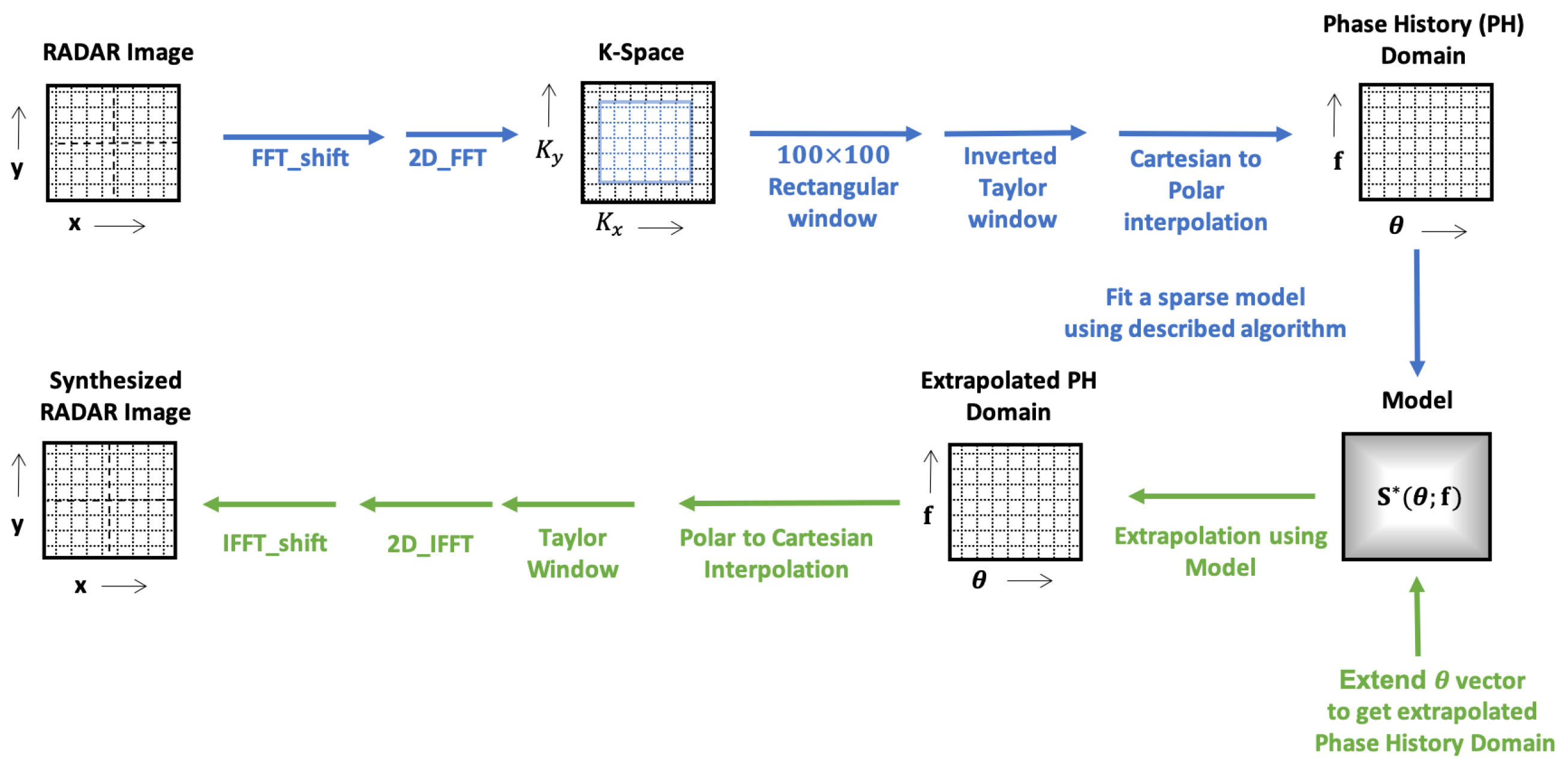
2.2. Modeling and Pose Synthesis Methodology
3. Experiments
3.1. MSTAR Data Set
3.2. Network Architecture
3.3. Experimental Setup
3.4. Determining Hyper Parameters
4. Results
4.1. Ablation Study of the Proposed Approach
4.2. Comparison with Existing SAR-ATR Models
5. Conclusions and Future Directions
Author Contributions
Funding
Data Availability Statement
Conflicts of Interest
References
- Moses, R.L.; Potter, L.C.; Cetin, M. Wide-angle SAR imaging. In Proceedings of the Algorithms for Synthetic Aperture Radar Imagery XI, Orlando, FL, USA, 12–16 April 2004; International Society for Optics and Photonics: Bellingham, WA, USA, 2004; Volume 5427, pp. 164–175. [Google Scholar]
- Potter, L.C.; Moses, R.L. Attributed scattering centers for SAR ATR. IEEE Trans. Image Process. 1997, 6, 79–91. [Google Scholar] [CrossRef]
- Çetin, M.; Stojanović, I.; Önhon, N.O.; Varshney, K.; Samadi, S.; Karl, W.C.; Willsky, A.S. Sparsity-Driven Synthetic Aperture Radar Imaging: Reconstruction, autofocusing, moving targets, and compressed sensing. IEEE Signal Process. Mag. 2014, 31, 27–40. [Google Scholar] [CrossRef]
- Potter, L.C.; Ertin, E.; Parker, J.T.; Cetin, M. Sparsity and Compressed Sensing in Radar Imaging. Proc. IEEE 2010, 98, 1006–1020. [Google Scholar] [CrossRef]
- Dungan, K.; Potter, L. Classifying transformation-variant attributed point patterns. Pattern Recognit. 2010, 43, 3805–3816. [Google Scholar] [CrossRef]
- Dungan, K.E.; Potter, L.C. Classifying Vehicles in Wide-Angle Radar Using Pyramid Match Hashing. IEEE J. Sel. Top. Signal Process. 2011, 5, 577–591. [Google Scholar] [CrossRef]
- Abdelrahman, T.; Ertin, E. Mixture of factor analyzers models of appearance manifolds for resolved SAR targets. In Proceedings of the Algorithms for Synthetic Aperture Radar Imagery XXII, Baltimore, MD, USA, 23 April 2015; International Society for Optics and Photonics: Bellingham, WA, USA, 2015; Volume 9475, p. 94750G. [Google Scholar]
- Hegde, C.; Sankaranarayanan, A.C.; Yin, W.; Baraniuk, R.G. NuMax: A Convex Approach for Learning Near-Isometric Linear Embeddings. IEEE Trans. Signal Process. 2015, 63, 6109–6121. [Google Scholar] [CrossRef][Green Version]
- Teng, D.; Ertin, E. WALD-Kernel: A method for learning sequential detectors. In Proceedings of the 2016 IEEE Statistical Signal Processing Workshop (SSP), Palma de Mallorca, Spain, 26–29 June 2016; pp. 1–5. [Google Scholar] [CrossRef]
- Cui, J.; Gudnason, J.; Brookes, M. Hidden Markov models for multi-perspective radar target recognition. In Proceedings of the 2008 IEEE Radar Conference, Rome, Italy, 26–30 May 2008; pp. 1–5. [Google Scholar] [CrossRef]
- Lecun, Y.; Bottou, L.; Bengio, Y.; Haffner, P. Gradient-based learning applied to document recognition. Proc. IEEE 1998, 86, 2278–2324. [Google Scholar] [CrossRef]
- Krizhevsky, A.; Sutskever, I.; Hinton, G.E. ImageNet Classification with Deep Convolutional Neural Networks. Commun. ACM 2017, 60, 84–90. [Google Scholar] [CrossRef]
- Hinton, G.E.; Salakhutdinov, R.R. Reducing the Dimensionality of Data with Neural Networks. Science 2006, 313, 504–507. [Google Scholar] [CrossRef]
- Chen, S.; Wang, H.; Xu, F.; Jin, Y. Target Classification Using the Deep Convolutional Networks for SAR Images. IEEE Trans. Geosci. Remote Sens. 2016, 54, 4806–4817. [Google Scholar] [CrossRef]
- Zhong, Y.; Ettinger, G. Enlightening deep neural networks with knowledge of confounding factors. In Proceedings of the IEEE International Conference on Computer Vision, Venice, Italy, 22–29 October 2017; pp. 1077–1086. [Google Scholar]
- Russakovsky, O.; Deng, J.; Su, H.; Krause, J.; Satheesh, S.; Ma, S.; Huang, Z.; Karpathy, A.; Khosla, A.; Bernstein, M.; et al. ImageNet Large Scale Visual Recognition Challenge. Int. J. Comput. Vis. (IJCV) 2015, 115, 211–252. [Google Scholar] [CrossRef]
- Yosinski, J.; Clune, J.; Bengio, Y.; Lipson, H. How transferable are features in deep neural networks? In Proceedings of the Advances in Neural Information Processing Systems, Montreal, QC, Canada, 8–13 December 2014; pp. 3320–3328. [Google Scholar]
- Oquab, M.; Bottou, L.; Laptev, I.; Sivic, J. Learning and transferring mid-level image representations using convolutional neural networks. In Proceedings of the IEEE Conference on Computer Vision and Pattern Recognition, Columbus, OH, USA, 23–28 June 2014; pp. 1717–1724. [Google Scholar]
- Simonyan, K.; Zisserman, A. Very Deep Convolutional Networks for Large-Scale Image Recognition. arXiv 2014, arXiv:1409.1556. [Google Scholar]
- Gunasekar, S.; Lee, J.; Soudry, D.; Srebro, N. Characterizing Implicit Bias in Terms of Optimization Geometry. In Proceedings of the 35th International Conference on Machine Learning, Stockholm, Sweden, 10–15 July 2018; Volume 80, pp. 1832–1841. [Google Scholar]
- Ruhi, N.A.; Hassibi, B. Stochastic Gradient/Mirror Descent: Minimax Optimality and Implicit Regularization. In Proceedings of the 7th International Conference on Learning Representations, ICLR 2019, New Orleans, LA, USA, 6–9 May 2019. [Google Scholar]
- Srivastava, N.; Hinton, G.; Krizhevsky, A.; Sutskever, I.; Salakhutdinov, R. Dropout: A simple way to prevent neural networks from overfitting. J. Mach. Learn. Res. 2014, 15, 1929–1958. [Google Scholar]
- Ioffe, S.; Szegedy, C. Batch normalization: Accelerating deep network training by reducing internal covariate shift. arXiv 2015, arXiv:1502.03167. [Google Scholar]
- Neyshabur, B.; Li, Z.; Bhojanapalli, S.; LeCun, Y.; Srebro, N. The role of over-parametrization in generalization of neural networks. In Proceedings of the 7th International Conference on Learning Representations, ICLR 2019, New Orleans, LA, USA, 6–9 May 2019. [Google Scholar]
- Pan, S.J.; Yang, Q. A survey on transfer learning. IEEE Trans. Knowl. Data Eng. 2009, 22, 1345–1359. [Google Scholar] [CrossRef]
- Huang, Z.; Pan, Z.; Lei, B. Transfer learning with deep convolutional neural network for SAR target classification with limited labeled data. Remote Sens. 2017, 9, 907. [Google Scholar] [CrossRef]
- Huang, Z.; Dumitru, C.O.; Pan, Z.; Lei, B.; Datcu, M. Classification of Large-Scale High-Resolution SAR Images with Deep Transfer Learning. IEEE Geosci. Remote Sens. Lett. 2021, 18, 107–111. [Google Scholar] [CrossRef]
- Zhou, F.; Wang, L.; Bai, X.; Hui, Y. SAR ATR of Ground Vehicles Based on LM-BN-CNN. IEEE Trans. Geosci. Remote Sens. 2018, 56, 7282–7293. [Google Scholar] [CrossRef]
- Zhang, F.; Wang, Y.; Ni, J.; Zhou, Y.; Hu, W. SAR Target Small Sample Recognition Based on CNN Cascaded Features and AdaBoost Rotation Forest. IEEE Geosci. Remote Sens. Lett. 2020, 17, 1008–1012. [Google Scholar] [CrossRef]
- Pei, J.; Huang, Y.; Sun, Z.; Zhang, Y.; Yang, J.; Yeo, T.S. Multiview Synthetic Aperture Radar Automatic Target Recognition Optimization: Modeling and Implementation. IEEE Trans. Geosci. Remote Sens. 2018, 56, 6425–6439. [Google Scholar] [CrossRef]
- Zhang, T.; Zhang, X. A polarization fusion network with geometric feature embedding for SAR ship classification. Pattern Recognit. 2022, 123, 108365. [Google Scholar] [CrossRef]
- Shao, Z.; Zhang, T.; Ke, X. A Dual-Polarization Information-Guided Network for SAR Ship Classification. Remote Sens. 2023, 15, 2138. [Google Scholar] [CrossRef]
- Sugavanam, N.; Ertin, E.; Burkholder, R. Compressing bistatic SAR target signatures with sparse-limited persistence scattering models. IET Radar Sonar Navig. 2019, 13, 1411–1420. [Google Scholar] [CrossRef]
- Shao, J.; Qu, C.; Li, J.; Peng, S. A Lightweight Convolutional Neural Network Based on Visual Attention for SAR Image Target Classification. Sensors 2018, 18, 3039. [Google Scholar] [CrossRef] [PubMed]
- Chen, H.; Zhang, F.; Tang, B.; Yin, Q.; Sun, X. Slim and Efficient Neural Network Design for Resource-Constrained SAR Target Recognition. Remote Sens. 2018, 10, 1618. [Google Scholar] [CrossRef]
- Min, R.; Lan, H.; Cao, Z.; Cui, Z. A Gradually Distilled CNN for SAR Target Recognition. IEEE Access 2019, 7, 42190–42200. [Google Scholar] [CrossRef]
- Zhang, F.; Liu, Y.; Zhou, Y.; Yin, Q.; Li, H.C. A Lossless Lightweight CNN Design for SAR Target Recognition. Remote Sens. Lett. 2020, 11, 485–494. [Google Scholar] [CrossRef]
- Dong, G.; Wang, N.; Kuang, G. Sparse representation of monogenic signal: With application to target recognition in SAR images. IEEE Signal Process. Lett. 2014, 21, 952–956. [Google Scholar]
- Song, S.; Xu, B.; Yang, J. SAR target recognition via supervised discriminative dictionary learning and sparse representation of the SAR-HOG feature. Remote Sens. 2016, 8, 683. [Google Scholar] [CrossRef]
- Song, H.; Ji, K.; Zhang, Y.; Xing, X.; Zou, H. Sparse representation-based SAR image target classification on the 10-class MSTAR data set. Appl. Sci. 2016, 6, 26. [Google Scholar] [CrossRef]
- Huang, Y.; Liao, G.; Zhang, Z.; Xiang, Y.; Li, J.; Nehorai, A. SAR automatic target recognition using joint low-rank and sparse multiview denoising. IEEE Geosci. Remote Sens. Lett. 2018, 15, 1570–1574. [Google Scholar] [CrossRef]
- Yu, Q.; Hu, H.; Geng, X.; Jiang, Y.; An, J. High-Performance SAR Automatic Target Recognition Under Limited Data Condition Based on a Deep Feature Fusion Network. IEEE Access 2019, 7, 165646–165658. [Google Scholar] [CrossRef]
- Lin, Z.; Ji, K.; Kang, M.; Leng, X.; Zou, H. Deep convolutional highway unit network for SAR target classification with limited labeled training data. IEEE Geosci. Remote Sens. Lett. 2017, 14, 1091–1095. [Google Scholar] [CrossRef]
- Fu, Z.; Zhang, F.; Yin, Q.; Li, R.; Hu, W.; Li, W. Small sample learning optimization for ResNet based SAR target recognition. In Proceedings of the IGARSS 2018-2018 IEEE International Geoscience and Remote Sensing Symposium, Valencia, Spain, 22–27 July 2018; IEEE: Piscataway, NJ, USA, 2018; pp. 2330–2333. [Google Scholar]
- Yue, Z.; Gao, F.; Xiong, Q.; Wang, J.; Huang, T.; Yang, E.; Zhou, H. A Novel Semi-Supervised Convolutional Neural Network Method for Synthetic Aperture Radar Image Recognition. Cogn. Comput. 2021, 13, 795–806. [Google Scholar] [CrossRef]
- Wang, C.; Shi, J.; Zhou, Y.; Yang, X.; Zhou, Z.; Wei, S.; Zhang, X. Semisupervised Learning-Based SAR ATR via Self-Consistent Augmentation. IEEE Trans. Geosci. Remote Sens. 2021, 59, 4862–4873. [Google Scholar] [CrossRef]
- Chen, K.; Pan, Z.; Huang, Z.; Hu, Y.; Ding, C. Learning from Reliable Unlabeled Samples for Semi-Supervised SAR ATR. IEEE Geosci. Remote Sens. Lett. 2022, 19, 4512205. [Google Scholar] [CrossRef]
- Zhang, C.; Bengio, S.; Hardt, M.; Recht, B.; Vinyals, O. Understanding deep learning requires rethinking generalization. In Proceedings of the 5th International Conference on Learning Representations, ICLR 2017, Toulon, France, 24–26 April 2017. [Google Scholar]
- Goodfellow, I.; Bengio, Y.; Courville, A. Deep Learning; MIT Press: Cambridge, MA, USA, 2016; Available online: http://www.deeplearningbook.org (accessed on 11 July 2023).
- Ding, J.; Chen, B.; Liu, H.; Huang, M. Convolutional neural network with data augmentation for SAR target recognition. IEEE Geosci. Remote Sens. Lett. 2016, 13, 364–368. [Google Scholar] [CrossRef]
- Yan, Y. Convolutional Neural Networks Based on Augmented Training Samples for Synthetic Aperture Radar Target Recognition. J. Electron. Imaging 2018, 27, 023024. [Google Scholar] [CrossRef]
- Marmanis, D.; Yao, W.; Adam, F.; Datcu, M.; Reinartz, P.; Schindler, K.; Wegner, J.D.; Stilla, U. Artificial generation of big data for improving image classification: A generative adversarial network approach on SAR data. arXiv 2017, arXiv:1711.02010. [Google Scholar]
- Lewis, B.; DeGuchy, O.; Sebastian, J.; Kaminski, J. Realistic SAR Data Augmentation Using Machine Learning Techniques. In Proceedings of the Algorithms for Synthetic Aperture Radar Imagery XXVI, Baltimore, MD, USA, 18 April 2019; SPIE: Bellingham, WA, USA, 2019; Volume 10987, pp. 12–28. [Google Scholar] [CrossRef]
- Gao, F.; Yang, Y.; Wang, J.; Sun, J.; Yang, E.; Zhou, H. A deep convolutional generative adversarial networks (DCGANs)-based semi-supervised method for object recognition in synthetic aperture radar (SAR) images. Remote Sens. 2018, 10, 846. [Google Scholar] [CrossRef]
- Cui, Z.; Zhang, M.; Cao, Z.; Cao, C. Image Data Augmentation for SAR Sensor via Generative Adversarial Nets. IEEE Access 2019, 7, 42255–42268. [Google Scholar] [CrossRef]
- Sun, Y.; Wang, Y.; Liu, H.; Wang, N.; Wang, J. SAR Target Recognition with Limited Training Data Based on Angular Rotation Generative Network. IEEE Geosci. Remote Sens. Lett. 2020, 17, 1928–1932. [Google Scholar] [CrossRef]
- Shi, X.; Zhou, F.; Yang, S.; Zhang, Z.; Su, T. Automatic Target Recognition for Synthetic Aperture Radar Images Based on Super-Resolution Generative Adversarial Network and Deep Convolutional Neural Network. Remote Sens. 2019, 11, 135. [Google Scholar] [CrossRef]
- Cha, M.; Majumdar, A.; Kung, H.; Barber, J. Improving SAR automatic target recognition using simulated images under deep residual refinements. In Proceedings of the 2018 IEEE International Conference on Acoustics, Speech and Signal Processing (ICASSP), Calgary, AB, Canada, 15–20 April 2018; IEEE: Piscataway, NJ, USA, 2018; pp. 2606–2610. [Google Scholar]
- Zhai, Y.; Ma, H.; Liu, J.; Deng, W.; Shang, L.; Sun, B.; Jiang, Z.; Guan, H.; Zhi, Y.; Wu, X.; et al. SAR ATR with full-angle data augmentation and feature polymerisation. J. Eng. 2019, 2019, 6226–6230. [Google Scholar] [CrossRef]
- Lv, J.; Liu, Y. Data Augmentation Based on Attributed Scattering Centers to Train Robust CNN for SAR ATR. IEEE Access 2019, 7, 25459–25473. [Google Scholar] [CrossRef]
- Agarwal, T.; Sugavanam, N.; Ertin, E. Sparse signal models for data augmentation in deep learning ATR. In Proceedings of the 2020 IEEE Radar Conference (RadarConf20), Florence, Italy, 21–25 September 2020; IEEE: Piscataway, NJ, USA, 2020; pp. 1–6. [Google Scholar]
- Sugavanam, N.; Ertin, E. Limited persistence models for SAR automatic target recognition. In Proceedings of the Algorithms for Synthetic Aperture Radar Imagery XXIV, Anaheim, CA, USA, 13 April 2017; International Society for Optics and Photonics: Bellingham, WA, USA, 2017; Volume 10201, p. 102010M. [Google Scholar]
- Sugavanam, N.; Ertin, E.; Burkholder, R. Approximating Bistatic SAR Target Signatures with Sparse Limited Persistence Scattering Models. In Proceedings of the International Conference on Radar, Brisbane, Australia, 27–31 August 2018. [Google Scholar]
- Sugavanam, N.; Ertin, E. Models of anisotropic scattering for 3D SAR reconstruction. In Proceedings of the 2022 IEEE Radar Conference (RadarConf22), New York, NY, USA, 21–25 March 2022; IEEE: Piscataway, NJ, USA, 2022; pp. 1–6. [Google Scholar]
- Sugavanam, N.; Ertin, E. Interrupted SAR imaging with limited persistence scattering models. In Proceedings of the 2017 IEEE Radar Conference (RadarConf), Seattle, WA, USA, 8–12 May 2017; IEEE: Piscataway, NJ, USA, 2017; pp. 1770–1775. [Google Scholar]
- Sugavanam, N.; Ertin, E. Recovery guarantees for MIMO radar using multi-frequency LFM waveform. In Proceedings of the 2016 IEEE Radar Conference (RadarConf), Philadelphia, PA, USA, 2–6 May 2016; IEEE: Piscataway, NJ, USA, 2016; pp. 1–6. [Google Scholar]
- Sugavanam, N.; Ertin, E. Recovery Guarantees for High-Resolution Radar Sensing with Compressive Illumination. In Compressive Sensing of Earth Observations; CRC Press: Boca Raton, FL, USA, 2017; pp. 83–104. [Google Scholar]
- Sugavanam, N.; Baskar, S.; Ertin, E. High Resolution MIMO Radar Sensing With Compressive Illuminations. IEEE Trans. Signal Process. 2022, 70, 1448–1463. [Google Scholar] [CrossRef]
- Brito, A.E.; Chan, S.H.; Cabrera, S.D. SAR image formation using 2D reweighted minimum norm extrapolation. In Proceedings of the Algorithms for Synthetic Aperture Radar Imagery VI, Orlando, FL, USA, 5–9 April 1999; International Society for Optics and Photonics: Bellingham, WA, USA, 1999; Volume 3721, pp. 78–91. [Google Scholar]
- Cetin, M. Feature-Enhanced Synthetic Aperture Radar Imaging. Ph.D. Thesis, Boston University, Boston, MA, USA, 2001. [Google Scholar]
- Jackson, J.A.; Rigling, B.D.; Moses, R.L. Canonical Scattering Feature Models for 3D and Bistatic SAR. IEEE Trans. Aerosp. Electron. Syst. 2010, 46, 525–541. [Google Scholar] [CrossRef]
- Sarabandi, K.; Chiu, T.C. Optimum corner reflectors for calibration of imaging radars. IEEE Trans. Antennas Propag. 1996, 44, 1348–1361. [Google Scholar] [CrossRef]
- Potter, L.C.; Chiang, D.M.; Carriere, R.; Gerry, M.J. A GTD-based parametric model for radar scattering. IEEE Trans. Antennas Propag. 1995, 43, 1058–1067. [Google Scholar] [CrossRef]
- Rauhut, H.; Ward, R. Interpolation via weighted L1 minimization. Appl. Comput. Harmon. Anal. 2016, 40, 321–351. [Google Scholar] [CrossRef]
- Greengard, L.; Lee, J.Y. Accelerating the nonuniform fast Fourier transform. SIAM Rev. 2004, 46, 443–454. [Google Scholar] [CrossRef]
- Duijndam, A.; Schonewille, M. Nonuniform fast Fourier transform. Geophysics 1999, 64, 539–551. [Google Scholar] [CrossRef]
- Burns, B.L.; Cordaro, J.T. SAR image-formation algorithm that compensates for the spatially variant effects of antenna motion. In Proceedings of the Algorithms for Synthetic Aperture Radar Imagery, Orlando, FL, USA, 6–7 April 1994; International Society for Optics and Photonics: Bellingham, WA, USA, 1994; Volume 2230, pp. 14–24. [Google Scholar] [CrossRef]
- Luo, P.; Wang, X.; Shao, W.; Peng, Z. Towards Understanding Regularization in Batch Normalization. arXiv 2018, arXiv:1809.00846. [Google Scholar]
- Abadi, M.; Barham, P.; Chen, J.; Chen, Z.; Davis, A.; Dean, J.; Devin, M.; Ghemawat, S.; Irving, G.; Isard, M.; et al. Tensorflow: A system for large-scale machine learning. In Proceedings of the 12th USENIX Symposium on Operating Systems Design and Implementation (OSDI 16), Berkeley, CA, USA, 2–4 November 2016; pp. 265–283. [Google Scholar]
- Belloni, C.; Balleri, A.; Aouf, N.; Merlet, T.; Le Caillec, J.M. SAR image dataset of military ground targets with multiple poses for ATR. In Proceedings of the Target and Background Signatures III, Warsaw, Poland, 11–12 September 2017; SPIE: Bellingham, WA, USA, 2017; Volume 10432, pp. 218–225. [Google Scholar]
- Lewis, B.; Scarnati, T.; Sudkamp, E.; Nehrbass, J.; Rosencrantz, S.; Zelnio, E. A SAR dataset for ATR development: The Synthetic and Measured Paired Labeled Experiment (SAMPLE). In Proceedings of the Algorithms for Synthetic Aperture Radar Imagery XXVI, Baltimore, MD, USA, 18 April 2019; SPIE: Bellingham, WA, USA, 2019; Volume 10987, pp. 39–54. [Google Scholar]
- Huang, L.; Liu, B.; Li, B.; Guo, W.; Yu, W.; Zhang, Z.; Yu, W. OpenSARShip: A dataset dedicated to Sentinel-1 ship interpretation. IEEE J. Sel. Top. Appl. Earth Obs. Remote Sens. 2017, 11, 195–208. [Google Scholar] [CrossRef]
- Sarroff, A.M. Complex Neural Networks for Audio. Ph.D. Thesis, Dartmouth College, Hanover, NH, USA, 2018. [Google Scholar]
- Jojoa, M.; Garcia-Zapirain, B.; Percybrooks, W. A Fair Performance Comparison between Complex-Valued and Real-Valued Neural Networks for Disease Detection. Diagnostics 2022, 12, 1893. [Google Scholar] [CrossRef]


| Sub-Sampling Ratio () | Baseline Data (B) | Adding Our Sub-Pixel Shifts (B + S) | Adding Our Poses and Sub-Pixel Shifts (B + S + P) | Full-Data Features (F) |
|---|---|---|---|---|
| 0.50 | 0.58 | 0.37 | 0.50 | |
| 1.44 ± 0.33 | 1.03 ± 0.08 | 0.54 ± 0.00 | 0.72 ± 0.06 | |
| 4.21 ± 0.83 | 2.33 ± 0.33 | 1.00 ± 0.34 | 0.99 ± 0.17 | |
| 10.99 ± 0.73 | 5.68 ± 0.67 | 3.32 ± 1.31 | 1.22 ± 0.26 | |
| 18.78 ± 2.40 | 14.02 ± 0.28 | 7.33 ± 0.54 | 2.07 ± 0.21 | |
| 32.38 ± 2.93 | 29.98 ± 2.62 | 18.66 ± 3.22 | 4.55 ± 0.57 |
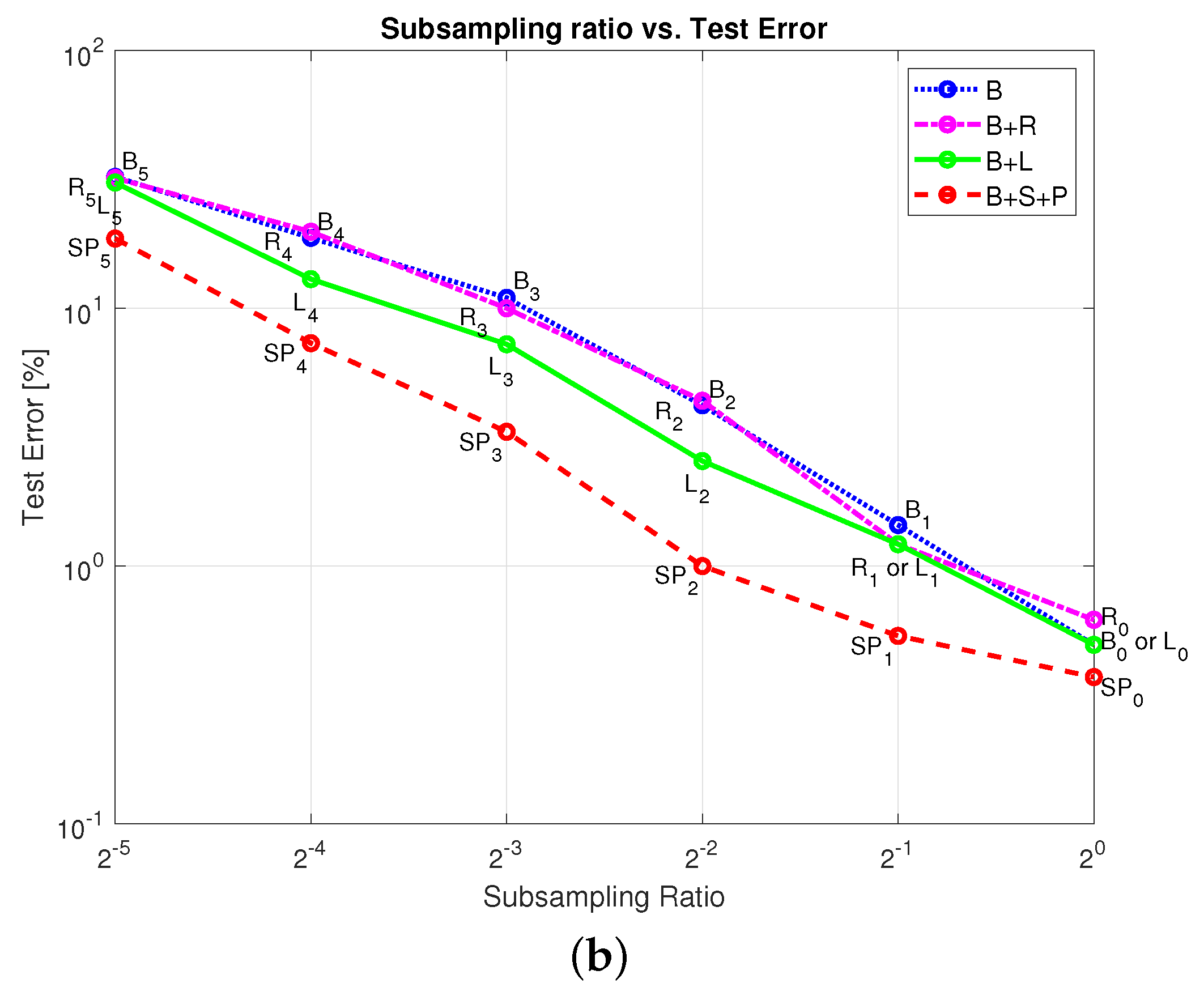
| Sub-Sampling Ratio () | Baseline Data (B) | Augmenting with Naively Rotated Poses (B + R) | Augmenting with Linearly Interpolated Poses (B + L) | Augmenting with Our Poses and Sub-Pixel Shifts (B + S + P) |
|---|---|---|---|---|
| 0.50 | 0.62 | 0.50 | 0.37 | |
| 1.44 ± 0.33 | 1.22 ± 0.19 | 1.22 ± 0.14 | 0.54 ± 0.00 | |
| 4.21 ± 0.83 | 4.38 ± 0.72 | 2.56 ± 0.21 | 1.00 ± 0.34 | |
| 10.99 ± 0.73 | 10.01 ± 1.72 | 7.26 ± 2.56 | 3.32 ± 1.31 | |
| 18.78 ± 2.40 | 19.83 ± 2.21 | 12.99 ± 1.10 | 7.33 ± 0.54 | |
| 32.38 ± 2.93 | 32.05 ± 7.58 | 30.79 ± 3.04 | 18.66 ± 3.22 |
| Class | 2S1 | BMP2 | BRDM2 | BTR60 | BTR70 | D7 | T62 | T72 | ZIL131 | ZSU234 | Error (%) |
|---|---|---|---|---|---|---|---|---|---|---|---|
| 2S1 | 196 | 0 | 1 | 0 | 3 | 1 | 40 | 5 | 18 | 10 | 28.467 |
| BMP2 | 21 | 117 | 2 | 18 | 10 | 0 | 1 | 23 | 3 | 0 | 40.0 |
| BRDM2 | 9 | 1 | 256 | 1 | 0 | 1 | 0 | 0 | 6 | 0 | 6.569 |
| BTR60 | 2 | 2 | 4 | 161 | 10 | 3 | 2 | 4 | 4 | 3 | 17.436 |
| BTR70 | 21 | 13 | 1 | 23 | 130 | 1 | 0 | 6 | 0 | 1 | 33.673 |
| D7 | 0 | 0 | 0 | 0 | 0 | 264 | 1 | 0 | 7 | 2 | 3.65 |
| T62 | 5 | 0 | 0 | 2 | 0 | 1 | 234 | 4 | 22 | 5 | 14.286 |
| T72 | 5 | 2 | 0 | 3 | 0 | 1 | 16 | 164 | 5 | 0 | 16.327 |
| ZIL131 | 1 | 0 | 0 | 0 | 0 | 34 | 4 | 0 | 234 | 1 | 14.599 |
| ZSU234 | 0 | 0 | 0 | 0 | 0 | 17 | 11 | 0 | 29 | 217 | 20.803 |
| Overall | 18.639 | ||||||||||
| Class | 2S1 | BMP2 | BRDM2 | BTR60 | BTR70 | D7 | T62 | T72 | ZIL131 | ZSU234 | Error (%) |
|---|---|---|---|---|---|---|---|---|---|---|---|
| 2S1 | 251 | 0 | 0 | 1 | 0 | 1 | 9 | 8 | 4 | 0 | 8.394 |
| BMP2 | 4 | 169 | 0 | 4 | 0 | 0 | 4 | 12 | 1 | 1 | 13.333 |
| BRDM2 | 16 | 8 | 243 | 0 | 0 | 0 | 0 | 0 | 6 | 1 | 11.314 |
| BTR60 | 2 | 1 | 4 | 172 | 6 | 1 | 3 | 1 | 1 | 4 | 11.795 |
| BTR70 | 7 | 2 | 1 | 0 | 184 | 0 | 0 | 2 | 0 | 0 | 6.122 |
| D7 | 0 | 0 | 0 | 0 | 0 | 263 | 0 | 0 | 0 | 11 | 4.015 |
| T62 | 6 | 0 | 0 | 4 | 0 | 1 | 257 | 4 | 1 | 0 | 5.861 |
| T72 | 1 | 0 | 0 | 0 | 0 | 0 | 10 | 183 | 0 | 2 | 6.633 |
| ZIL131 | 6 | 0 | 0 | 0 | 0 | 8 | 6 | 1 | 244 | 9 | 10.949 |
| ZSU234 | 0 | 0 | 0 | 0 | 0 | 0 | 2 | 0 | 0 | 272 | 0.73 |
| Overall | 7.711 | ||||||||||
| Method | Error (%) Using 100% Data | Error (%) Using ≤20% Data |
|---|---|---|
| SVM (2016) [40] | 13.27 | 47.75 (at ) |
| SRC (2016) [40] | 10.24 | 36.35 (at ) |
| A-ConvNet (2016) [14] | 0.87 | 35.90 (at ) |
| Ensemble DCHUN (2017) [43] | 0.91 | 25.94 (at ) |
| CNN-TL-bypass (2017) [26] | 0.91 | 2.85 (at ) |
| ResNet (2018) [44] | 0.33 | 5.70 (at ) |
| DFFN (2019) [42] | 0.17 | 7.71 (at ) |
| Our Method | 0.37 | 1.53 (at ) |
Disclaimer/Publisher’s Note: The statements, opinions and data contained in all publications are solely those of the individual author(s) and contributor(s) and not of MDPI and/or the editor(s). MDPI and/or the editor(s) disclaim responsibility for any injury to people or property resulting from any ideas, methods, instructions or products referred to in the content. |
© 2023 by the authors. Licensee MDPI, Basel, Switzerland. This article is an open access article distributed under the terms and conditions of the Creative Commons Attribution (CC BY) license (https://creativecommons.org/licenses/by/4.0/).
Share and Cite
Agarwal, T.; Sugavanam, N.; Ertin, E. Sparse Signal Models for Data Augmentation in Deep Learning ATR. Remote Sens. 2023, 15, 4109. https://doi.org/10.3390/rs15164109
Agarwal T, Sugavanam N, Ertin E. Sparse Signal Models for Data Augmentation in Deep Learning ATR. Remote Sensing. 2023; 15(16):4109. https://doi.org/10.3390/rs15164109
Chicago/Turabian StyleAgarwal, Tushar, Nithin Sugavanam, and Emre Ertin. 2023. "Sparse Signal Models for Data Augmentation in Deep Learning ATR" Remote Sensing 15, no. 16: 4109. https://doi.org/10.3390/rs15164109
APA StyleAgarwal, T., Sugavanam, N., & Ertin, E. (2023). Sparse Signal Models for Data Augmentation in Deep Learning ATR. Remote Sensing, 15(16), 4109. https://doi.org/10.3390/rs15164109