Article

Solid Precipitation and Visibility Measurements at the Centre for Atmospheric Research Experiments in Southern Ontario and Bratt’s Lake in Southern Saskatchewan

by
Faisal S. Boudala
1,* and
Jason A. Milbrandt
2
1
Meteorological Research Division, Environment and Climate Change Canada, North York, ON M3H 5T4, Canada
2
Meteorological Research Division, Environment and Climate Change Canada, Dorval, QC H9P 1J3, Canada
*
Author to whom correspondence should be addressed.
Remote Sens. 2023, 15(16), 4079; https://doi.org/10.3390/rs15164079
Submission received: 26 June 2023 / Revised: 10 August 2023 / Accepted: 12 August 2023 / Published: 18 August 2023
(This article belongs to the Section Atmospheric Remote Sensing)

Abstract

:
Accurate measurement of solid precipitation ( S ) has a critical importance for proper understanding of the Earth’s hydrological cycle, validation of emerging technologies and weather prediction models, and developing parameterizations of severe weather elements such as visibility ( V i s ). However, measuring S is still a challenging problem, due mainly to wind effects. The wind effects are normally mitigated by using a Double-Fence Automated Reference (DFAR) system to reduce the wind speed ( U g ). To contribute towards addressing some of these problems, we have analyzed datasets collected at two sites, Center for Atmospheric Research Experiments (CARE) and Bratt’s Lake, located in southern Ontario and southern Saskatchewan, Canada, respectively, using several instruments. The instruments at CARE include two Geonor gauges, one placed inside a DFAR ( S D F A R ) and the other inside a double Alter shield ( D A S G ), a Pluvio2 gauge inside a single Alter shield ( S A S P ), a HotPlate, a PARSIVEL2 disdrometer that measures S and fall velocity ( V ), and an FD12P senor that measures S and type and Vis. The instruments deployed in Bratt’s Lake includes a similar DFAR system and DAS Pluvio2 gauge. The results show that for the U g observed in this study ( U g < 6 ms−1), both D A S G and S A S P have similar collection efficiency (CE) of near 70%. The transfer functions (TF) for D A S G and S A S P as a function of U g and also U g , and V were derived. The TF developed for the D A S G that includes both U g and V showed better agreement with observation than just U g alone. The TF developed for D A S G at CARE site was tested using the data collected in Bratt’s Lake and correlated well (R = 0.86), but slightly overestimated the S accumulation by about 12%. The S measured at CARE site using all the other instruments were correlated well with   S D F A R (R = 0.9), but the PARSIVEL2 and FD12P overestimated and underestimated the snow amount, respectively, as compared the S D F A R . However, the HotPlate captured similar amount of S as the S D F A R . According to this study, the S D F A R showed good correlation with Vis.

1. Introduction

Accurate measurement of solid precipitation (S) is critical for understanding of the hydrological cycle and validation of numerical weather prediction (NWP) models, particularly for severe weather forecasting and nowcasting applications that are relevant for aviation and ground transportation. Reduction in visibility (Vis) due to snow is one of the major causes of aviation related delays [1] and ground transportation accidents [2,3].). In fact, solid precipitation intensity is estimated based on visibility, particularly for aviation application [4,5]. Many of the current NWP models parameterize Vis in terms of S [4,5,6]. These parameterizations were mainly developed based on low temporal resolution (e.g., hourly, daily) manually determined S or non-standard snow gauge data. Developing a better parametrization is also challenging due to the difficulty associated with characterization of scattering properties of snow particles [4,5,7].
One of the ways to mitigate the effects of wind speed that normally diminishes the catch efficiency of many traditional snow gauges is by using a standard wind shied referred to as Double Fence Intercomparison Reference (DFIR) as recommended by the World Meteorological Organization (WMO) [8] (see Figure 1). Using this as a reference, correction or adjustment factors normally referred to as transfer functions (TF) of various precipitation gauges without or with shields (single or double Alter) can be developed. Previously, these transfer functions were derived based on coarse time resolution data (e.g., daily accumulated precipitation data) [8,9]. Currently there are a number of studies of solid precipitation catch efficiency of automated Geonor or Pluvio2 gauge with a single Alter shield configuration set to collect data at high temporal resolution [10,11,12,13]. These studies are also mainly related to the effects of wind speed normally captured using some type of adjustment or TF as summarized in recent publications [12,14].
Using the Solid Precipitation Intercomparison Experiment (SPICE) datasets collected from eight different sites in Europe, US, and Canada including CARE site, the authors of [10] developed TFs as a function of wind speed and temperature and wind speed alone for a single Alter shielded (SAS) Geonor and Pluvio2 gauges by combining the data from these sites. The TF derived using the combined datasets were referred to as a universal TF (see in Table 1). When this universal TF was tested using data collected from different climate regions, however, it showed significate variability from site to site in the adjustment error indicating the influence of local climatology ([10,15]). The functional form used to parameterize the catch efficiency, particularly related to wind speed alone has a tendency to unrealistically over-predict the catch efficiency at low wind speeds [16]. A similar TF using temperature and wind speed was also developed for a SAS Geonor gauge based on Bayesian analysis approach using data collected in [17]. The authors of [18], however, suggested to use precipitation intensity in place of temperature and developed collection efficiency as a function of precipitation intensity and wind speed for a SAS Geonor gauge and found that their approach gave better results than the one that included temperature. There are, however, relatively limited studies of catch efficiency of the automated Geonor with double Alter shield configuration [11,19]. The authors of [19], developed a TF for double Alter shielded (DAS) Geonor (given Table 1) using data collected at Marshall site in the US. The authors of [11] developed transfer functions as a function of wind speed and temperature for both DAS Geonor and Pluvio2 gauges. Although there are a number of studies that considered such as temperature and precipitation intensity in addition to wind speed, the catch efficiency or TFs that explicitly consider other parameters such as fall velocity are also limited in the literature, particularly based on in situ measurements ([20,21].
Using the CARE site data and computational fluid dynamics modeling (CFDM), [21] developed TFs as a function of both wind and fall velocity for unshielded Geonor gauge and showed the addition of fall velocity improved the collection efficiency. Similarly [22] also developed a number of TFs as a function of wind speed and fall velocity using a CFDM for a SA Geonor gauge. More recently [20] developed a TF as a function of wind speed for two different fall velocity regions (V < 1.2 ms−1 and V > 1.2 ms−1) for a SA Geonor, but their TF does not explicitly include fall velocity. There is a continued interest to operationally use DAS gauges (Pluvio or Geonor) because of their ability capturing more falling snow particles than the SA gauges, and thus developing transfer function suitable for these types of gauges has a critical importance.
In order to test a number of TFs developed elsewhere and develop new and better TFs, high-time-resolution solid precipitation data collected at CARE, Ontario and Bratt’s Lake, Saskatchewan, Canada were analyzed. The datasets collected using an automated Geonor gauge placed inside a DFAR is used to develop and test the new TFs for Geonor and Pluvio2 gauges with a DAS and OTT Pluvio2 gauge with a SAS. The TFs are developed based on both wind speed and fall velocity and wind speed alone where the fall velocity measurements were available. A number of nontraditional precipitation sensors were also evaluated using the DFAR data. By taking advantage of the DFAR solid precipitation intensity data, new Vis parameterizations are also developed and compared against the one found in the literature. The paper is organized as follows: materials and methods are discussed in Section 2, the results are presented in Section 3, and the conclusions are given in Section 4.

2. Materials and Methods
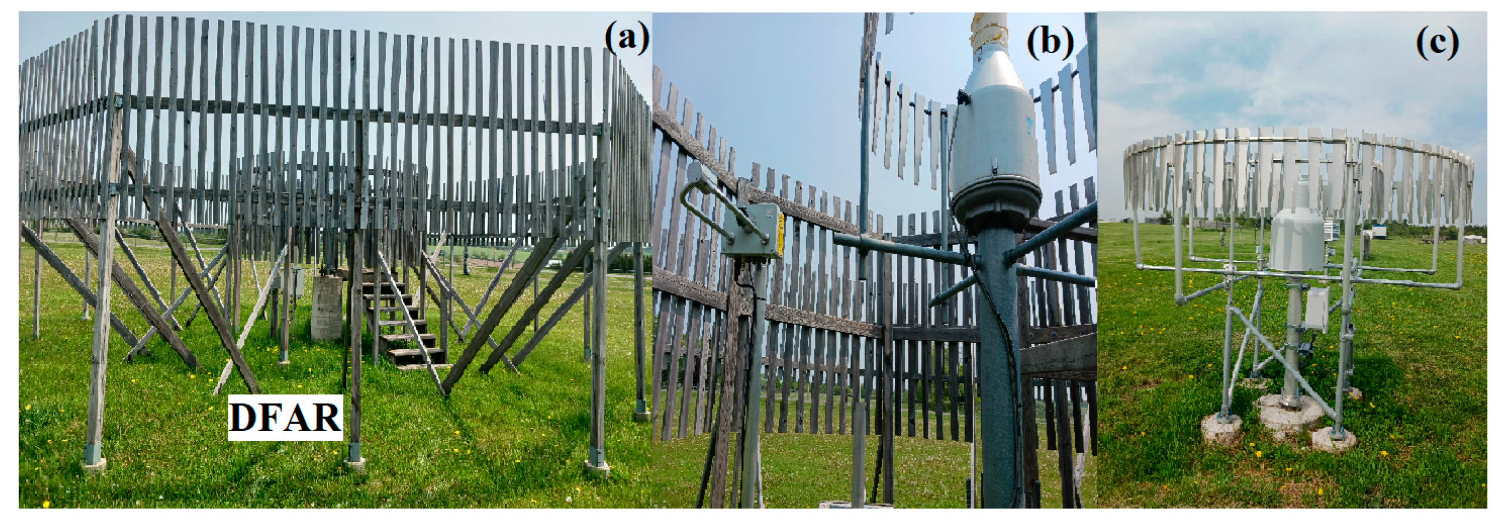
2.1. CARE Site

CARE site is located in Egbert, Ontario, Canada (44.23N, 79.78W, 251 m ASL). The area is influenced by lake effects mainly coming from Georgian Bay and Lake Huron from north, Lake Simcoe from the east and Lake Ontario to the south. The area is generally open farmland or pasture with some mixed forest trees and bushes surrounding the site and hence generally not very windy and as a result no significant blowing snow condition is expected. The typical weather conditions observed during the measurement period will be discussed later.

2.2. Bratt’s Lake Site

The Bratt’s Lake site on the other is located in southern Saskatchewan, Canada (50.16N, 104.68W, 585 ASL) and generally situated in an exposed open field with no bushes or tress to reduce the wind field. A brief climatology of the area is given in [23]. It is characterized by cold winter with light snow and windy conditions that produces occasional blowing snow with a mean wind speed of 4.4 ms1. The typical weather conditions during the measurement period considered in this study will be given later. The data collected at the site were primarily used as an independent dataset to test the transfer function developed using the CARE site data.

2.3. The Gauge Data Analysis

The Pluvio2 and Geonor gauge datasets used in this study are mainly based on data collected during 2012–2013 period at CARE site as part of the SPICE project [24] and also after the SPICE measurements at Baratt’s Lake during 2021–2022 period using DAS Pluvio2 [23,25]. The solid precipitation rate or accumulation being discussed in this paper is defined as liquid water equivalent (LWE) ([19,26]. The Geonor T-200B3 precipitation gauge used in this study is described in many publications including [10,11,19,20,25,26]. A brief description of the gauge is given Appendix A. The Geonor gauge with a SAS was installed at 3 m height inside an orthogonal double fence, the DFAR as shown in Figure 1 to minimize the effect of wind. The raw data contain precipitation accumulation corresponding to each wire calculated at 6 s time intervals. At such a high temporal resolution, the Geonor raw data can be quite noisy even with reduced wind effects, particularly under clear and light precipitation conditions, and hence requires careful assessment of each dataset. For this study we have selected mostly snow days based on measurements of present weather sensors and temperature measurements. The algorithm used for data analysis is described in [27]
The first step is removing any suspicious artifacts in the data by carefully analyzing the raw data each day. After removing the artifact, the data are de-noised using coefficients of Gaussian low-pass filter and zero-phase forward and reverse digital filtering method. The digitally filtered data are assessed for possible false precipitation events using the FD12P probe and if found they are removed from the data. The average of the three wires was used unless one of the wires deviated from the mean by twice the minimum standard deviation of one of the wires (see [27]). For precipitation type, wind speed and temperature studies, 10-min averaged data were used, for the catch efficiency study, 30-min averaged data were used, and for the precipitation data, less than 0.2 mm measured in 30 min were ignored. The threshold used for the gauge under test ( T g ) was determined using equation following [10] as
T g = m e d i a n P g P D F A R × 0.2 ,
where P g is the 30-min snow accumulation based on the gauge under test and the P D F A R   30-min accumulation of the DFAR reference system. Similar analysis was carried out using the Bratt’s Lake data. The detailed methods used to quality control the data is given in [23]. The physical description and operating principles of the OTT Pluvio2 200 gauge used in this study is also described in SPICE reports [24,26]. Brief description of the gauge is given in Appendix A.
The functional form of the collection efficiency (CE) for Geonor or Pluvio2 gauges generally follow [28] in a form
C E u g = 1 a   e x p b U g
or
CE u g , v = exp ( a U g b + c V d )
where U g is the wind speed at the gauge height level given in m s1, and V is the measured fall velocity is also in m s1, and a, b, c, and d are some constants determined using list square regression model. The functional form given in Equation (2) was chosen so that it will never exceed the CE from unity hence it has not limitation of overpricing the efficiency at low wind speeds. The correlations coefficients provided in this paper are the adjusted values. These results will be presented in Section 3.

2.4. Precipitation Intensity, Type, and Fall Velocity

Precipitation intensity and type were also measured using the Vaisala FD12P present weather sensor and he OTT PARSIVEL2 disdrometer. The precipitation intensity was also measured using the HotPlate sensor, and the fall velocity was obtained using the PARSIVEL2. These specialized instruments were deployed by the High Impact Weather Research (HIWR) section of the Meteorological Research Section of Environment and Climate Change Canada. The detailed descriptions of the FD12P are given in [5,29] and the PARSIVEL disdrometer probe is originally developed by [30] and also described in a number of publications [31,32] and references there in). The Yankees HotPlate is described in [33] as well as in [34]. In this paper, only brief descriptions of the instruments will be presented in Appendix A.

2.5. Visibility and Solid Precipitation Intensity Data Analysis

As discussed, accurate determination of solid precipitation has very important implications for nowcasting and forecasting of Vis during snowfall, particularly for aviation where Vis information is also used for aircraft ground operation. Although there is a weak temperature dependence, it is mainly the Vis data that are used to estimate solid precipitation intensity by assuming the existence of strong correlation between Vis and S . Thus, testing the validity of this assumption using the DFAR data has critical importance, particularly for aviation. In additions, since many of the traditional gauges used operationally and including those found in the airports utilized to measure solid precipitation are not well shielded, thus the TFs developed in this study can be used to perform catch efficiency adjustment of these gauges in order to calculate Vis accurately.
Some applications of the Vis   S relationship in aviation, for example, include under daytime and temperatures (T < −1 °C) conditions (that is consistent with Vis data used in this paper), the S thresholds adapted by Transport Canada (TC) based on Vis are: Very light (Vis > 3.219 km), light (1.408 km < Vis < 3.219 km), moderate (0.604 km < Vis < 1.408 km), and heavy (Vis ≤ 0.604 km) [35]. This information is used as a guideline for estimating aircraft holdover time and de-icing operation [35]. In the guidance table, the Vis data are also segregated according to daytime and nighttime conditions [35], and this issue is discussed extensively in the previous studies [4,36,37]. According to Boudala et al., (2012), the nighttime visibility ( V n ) can be related to daytime visibility ( V d ) as
V n = 1.31 V d 0.71 ,
where V d is given in km. Most automated present weather sensors including the FD12P used in this study are not equipped to distinguish between V d and V n as a result, they report Vis only relative to V d , but can be adjusted for nighttime condition using Equation (4).
There are no universally accepted thresholds for LWE solid precipitation intensity for application in aviation. In this study we use as a reference the LWE snow intensity thresholds as very light (0.3 < S < 0.4 m m h 1 ), light (0.4 < S < 1 m m h 1 ), moderate (1 < S < 2.5 m m h 1 ), and heavy (S ≥ 2.5 m m h 1 ), adapted by Society of Automotive Engineers (SAE) to select de-icing fluids [38].

3. Results

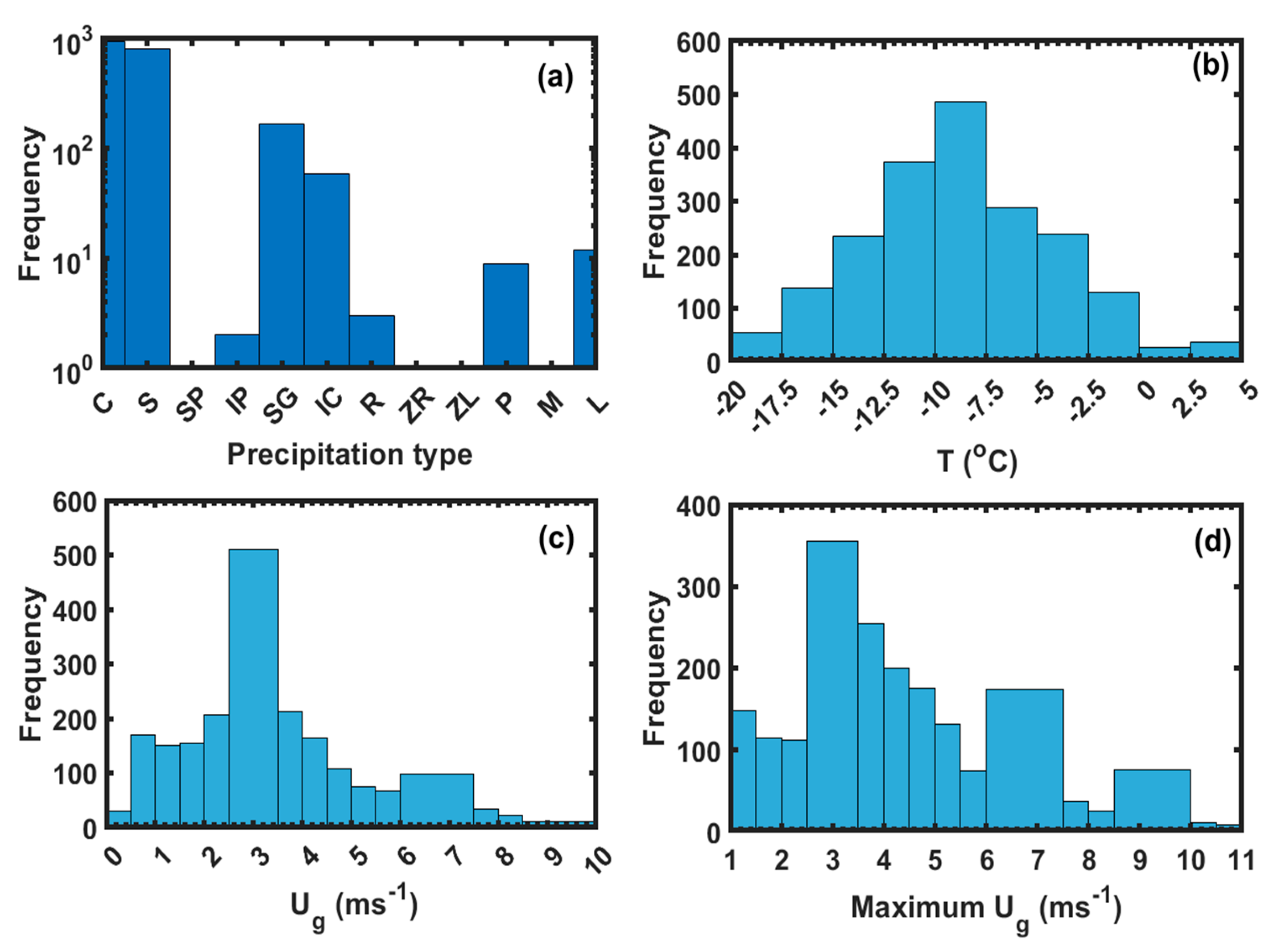
3.1. Precipitation Type and Temeprature at CARE Site
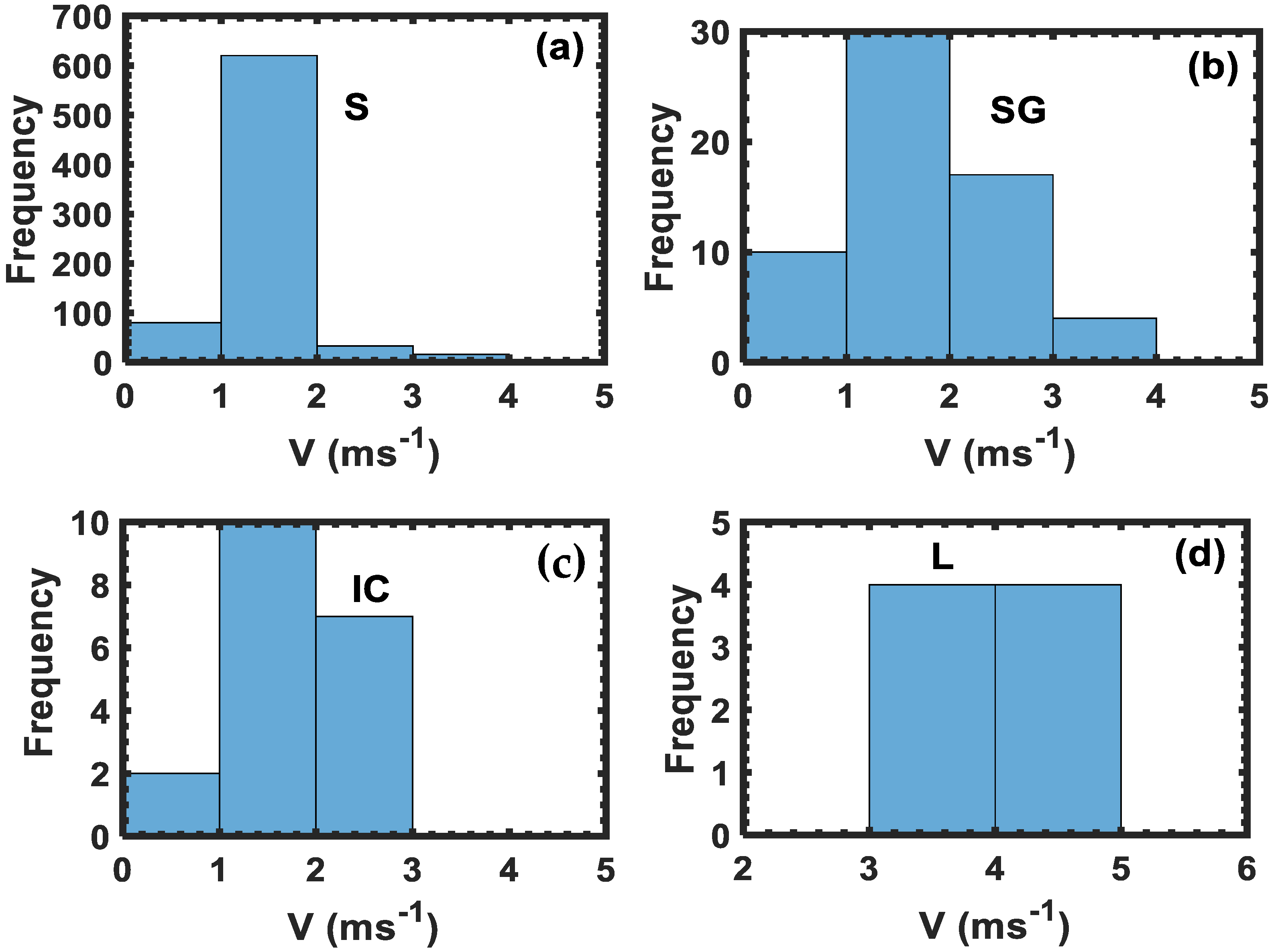
Figure 2 shows the distributions of most probable precipitation type within 10-min interval based on the FD12P probe (Figure 2a), 10-min averaged temperature (Figure 2b) and wind speed (Figure 2c), and maximum wind within 10-min time interval of 1-min averaged data (Figure 2d). Based on these results, the dominant precipitation type in this dataset is snow (S) followed by snow grains (SG) and ice crystals (IC). There have been a few rain (R) and drizzle (L) events, but no mixed-phase precipitation conditions were observed although the probe reported a few unknown precipitation types. The dominance of solid phase precipitation type is consistent with the distribution of temperature (Figure 2b) that shows mainly cold temperature conditions (−20 °C < T < 0 °C). It should be noted here that in these temperature ranges, it is possible to have mixed-phase supercooled icing condition, but for these studies all solid precipitation case datasets were chosen using both temperature and precipitation type measurements. The 10-min averaged wind speed measured using the Vaisala NWS425 ultrasonic wind sensor reached 8 m s−1, but the majority of wind speeds ranged between 2 and 4 ms−1 (Figure 2c), and the maximum wind events that exceeded 8 ms−1 occurred at relatively lower frequencies (Figure 2d). Nonetheless, as will be discussed later, these wind speeds are still quite significant for degrading the collection efficiency of the gauges being tested, but no significant blowing snow conditions are expected. Since the precipitation is measured at 6-s time intervals, the wind gust at such a high temporal resolution (not discussed here) could be quite significantly higher than the 1-min averaged wind speed (Figure 2d) that can potentially enhance the wind effect.

3.2. Fall Velocity

Figure 3 shows the distribution of 10-min averaged fall velocity ( V ) of different kind of solid precipitation types based on the PARSIVEL measurements (Figure 3a–c) including some drizzle events (Figure 3d). The dominant fall speeds of solid phase precipitation particles range 1–2 ms−1 and for the drizzle drops, the fall speeds were larger ranging between 3–4 ms−1. Particle fall velocity increases with increasing snow density and size [39] and studies show that snow catch efficiency improves with increasing fall velocity [18,20,40]. Note also that there are some overlaps of fall velocity between solid and drizzle particles. This is most likely related to size, particle habit, and snow density variations, as mentioned earlier, which normally complicate the fall velocity and size relationships. In this study the 30-min averaged fall velocity will be used for characterization of CE of a Geonor gauge, and this will be discussed in Section 3.3.

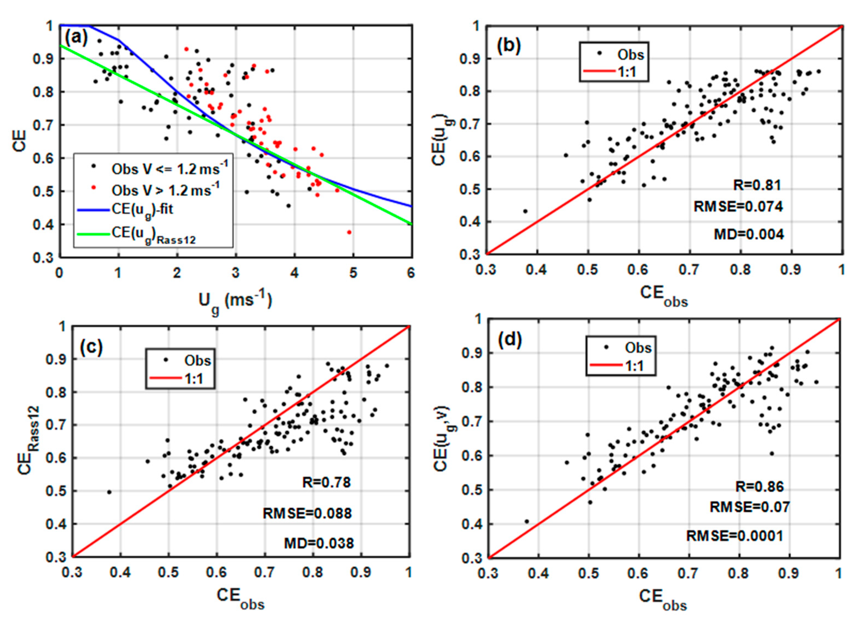
3.3. Solid Precipitation and Collection Efficiency of Geonor Gauge at CARE Site

Figure 4 shows collection efficiency of the Geonor gauge with a DAS segregated based on fall velocity values and two fitted curves as a function of U g alone based on this study ( C E U g - f i t ) and [19] ( C E U g R a s s 12 ) (see Table 1) (Figure 4a) and the associated comparisons against observation (Figure 4b,c). Based on these results, there is some evidence that particles having relatively higher fall velocities are captured better, particularly at higher wind speeds (Figure 4a) confirming the theoretical modeling studies [22,40] as well as measurements [20,21]. The comparisons of the two curves agree reasonably well with observation with correlation coefficient (R = 0.8), but the one based on [19] that was developed based on data at Marshall site in the US is slightly underestimated the efficiency with root mean square error (RMSE) value of 0.09 and mean difference (MD) (mean(Obs-fitted data) or mean bias of 0.04 as compared to 0.074 and 0.004, respectively (Figure 4b), particularly at lower wind speeds (Figure 4a,c). A TF that includes both U g and V is also derived using a multiple linear regression model and given in Table 1 and the comparison of this function against observation is shown in Figure 4d. Based on results showed in Figure 4d, the addition of fall velocity improves both the correlation coefficient and RMSE values as compared to those use wind speed alone (Figure 4b,c). As indicated in Figure 4b–d, it is evident that all the TFs systematically underestimate the CE between 0.8 and 0.9, which would be under calm conditions (1< U g < 2 ms−1) (Figure 4a), this is particularly evident in the Rass12 TF that tends to underestimate CE at wind speeds ( U g < 3 ms−1). These could be associated with many factors including uncertainty in the functional form of the TF under relatively calm conditions when the effect of wind is relatively low and other factors such as temperature and particle type can play some roles, but not properly captured in the TF.
Figure 5 shows the collection efficiency of none tradition optical probes the HotPlate (Figure 5a), Vaisala FD12P (Figure 5b), and PARIVEL2 (Figure 5c). As indicated in the figure, there is no well defined wind speed dependence of the collection efficiency of HotPlate or FD12P, particularly the FD12P as would be expected (Figure 5a,b). However, for HotPlate, there is a tendency of decreasing collection efficiency with wind speed for wind speeds ( U g < 3 m s−1) as indicated by the linear fit (R = 0.67), but for higher wind speeds no significant wind speed dependence as also shown with a poorly correlated (R = 0.2) linearly fitted line (Figure 5a), thus in this study no additional wind speed correction was applied as has been for example in Rasmussen et al., (2011). In case of the PARSIVEL, the collection efficiency slightly decreases with wind speeds ( U g < 3 ms−1), but increases with wind speed for wind speeds ( U g > 3 ms−1) and linearly fitted curves are also shown. Generally, the PARSIVEL disdrometer overestimates the solid precipitation rate for all wind speed range (Figure 5c) similar to studies reported earlier under very low wind speed conditions ([32]. These discrepancies could be also related to uncertainty related to derivation of precipitation intensity implemented in the internal algorithm used in the probe. This is particularly true for lower wind speeds ( U g < 3 ms−1) where the instrument overall showed overestimation of S. As discussed in [32], the use of different snow density–size relationships that resulted more reasonable solid precipitation intensities. In this study, no such modifications or assumptions were made for calculating the solid precipitation intensity based on the velocity and size spectra measurements.
Figure 6 show scattered plots and the best fit lines of the solid precipitation rates measured using the PARSIVEL2 (Figure 6a), HotPlate (Figure 6b), and FD12P (Figure 6c) against the S D F A R . All the intensities measured by all the instruments correlated quite well, with correlation coefficients (R) better than 0.9, but the PARSIVEL probe overestimates S from both light to high S as compared to the S D F A R (Figure 6a). The HotPlate, however, overestimates light values (S < 0.5 mm h−1), but underestimates S for values greater than 0.5 mm h−1 (Figure 6b). In contrast, the FD12P generally underestimates S for all solid precipitation range.
Figure 7 shows the accumulation (Figure 7a) and intensity of S (Figure 7b) based on all instruments and those adjusted (adj) based on unadjusted DAS Geonor, adjusted with a C E ( u g ) and C E ( u g , v ) represented by D A S u g and D A S u g v , respectively. The transfer function C E ( u g ) able to adjust the CE with a slight overestimation of S D F A R by about 6%. For the one based on the Marshall site data, D A S u g r a s s 12 was also able adjust the undercatch with a similar overestimation (8.2%) as compared to the S D F A R . The TF D A S u g v , however, adjusted the DAS gauge without any bias. The PARSIVEL2 overestimates the accumulation relative to the S D F A R by close to 28%. On the other hand, the accumulation based on the HotPlate is relatively quite close to the S D F A R with only 3.5% under estimation. The FD12P performed as well as the unadjusted DAS, but unadjusted DAS underestimates the snow accumulation as compared to the S D F A R by close to 32% which is similar to the estimated errors reported in the users’ manual.

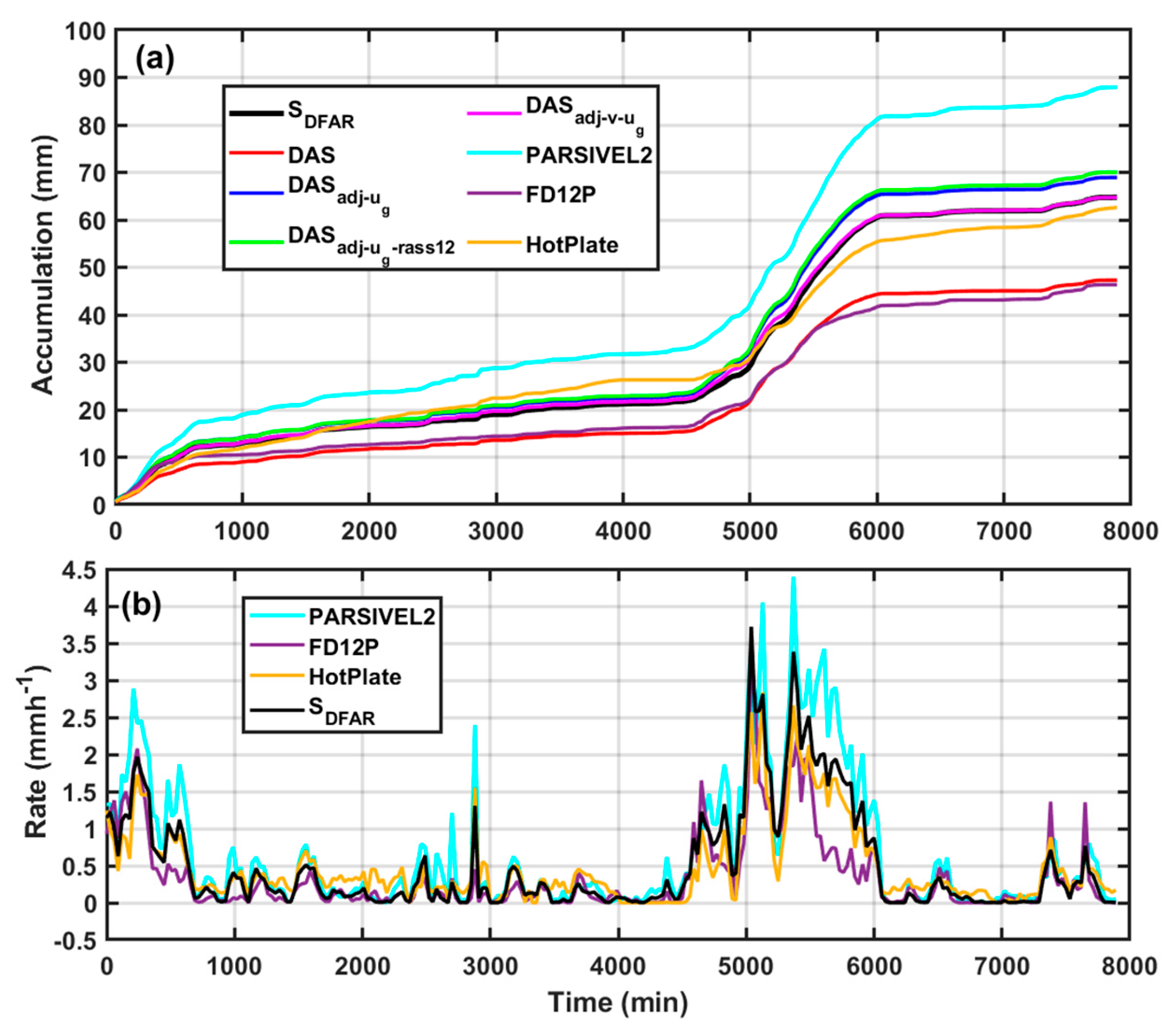
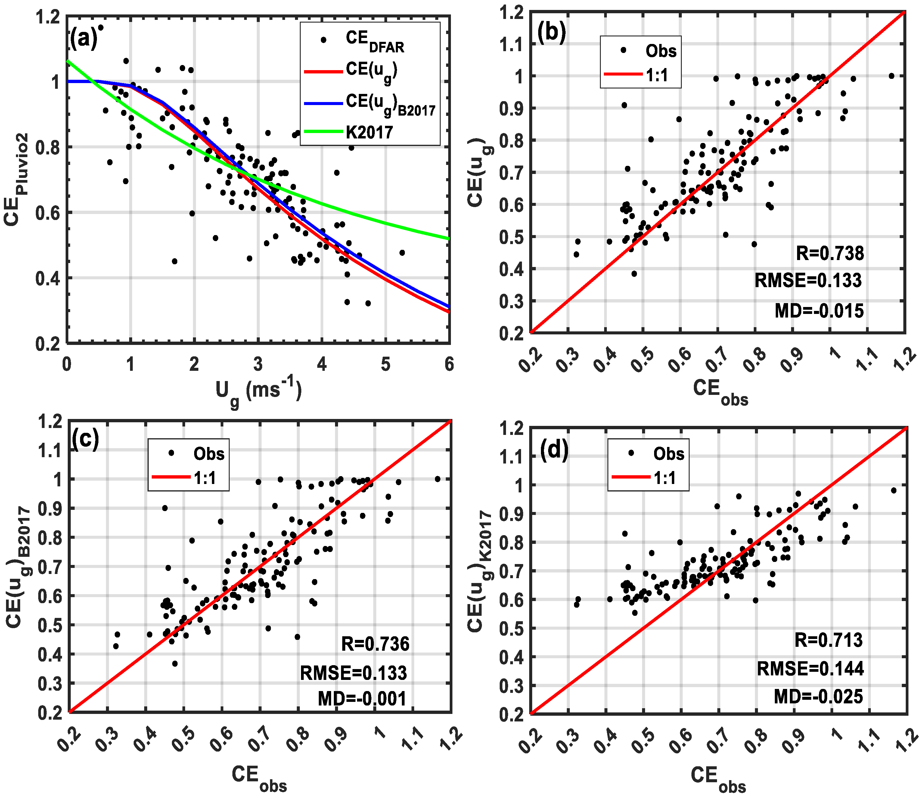
3.4. Solid Precipitation and Collection Efficiency of Pluvio2 Gauge at CARE Site

In order to compare collection efficiency of Pluvio2 with a SAS reported in [10,28] similar data analysis to Geonor gauge was performed and the results are given in Figure 8. The collection efficiency calculated here is relative to S D F A R and SAS Pluvio2 gauge. According to [10,11], S D F A R measured using Geonor and Pluvio2 were identical and hence the uncertainty associated with using the S D F A R as a reference is expected to be negligible. The collection efficiency of SAS Pluvio2 gauge derived based on data at Cold Lake, Alberta [28] ( C E u g B 2017 ) is identical to CE of SAS Pluvio2 ( C E u g   Figure 7a) and both are shown in Table 2. For comparison, the CE reported in [10] ( C E u g K 2017 ) is also shown. The functional form of this CE is different as compared to the one derived in this study and as a result there are some differences particularly at wind speeds ( U g > 3 ms−1 and U g   < 2 ms−1), but as will be discussed later both transfer functions gave very similar accumulation. The TF based on this study, B2017 and K2017 are given in Figure 8b–d, respectively. The correlation coefficients are similar (0.84–0.86), B2017 and the one derived in this study is slightly higher. The RMSE values are also similar (0.13–0.14), although the K2017 gave slightly higher MD or mean bias. It can be noted also the K2017 TF clearly shows overestimation of CE for CE < 0.6 and underestimation of CE for CE > 0.9.
Figure 9 Shows the accumulation based on S D F A R , SAS Pluvio2 without correction, and adjusted based on this study ( S A S u g ) ,   S A S u g B 2017 , and S A S u g K 2017 . As mentioned earlier all the collection efficiencies gave similar accumulations, although K2017 gave slightly lower accumulation by about 3% and including slight overestimation of B2017 (3.6%), the new CE based on this study gave a better result with only 0.85% difference. However, the unadjusted SAS Pluvio2 underestimated the S as compared to the S D F A R by about 31% based on this study.

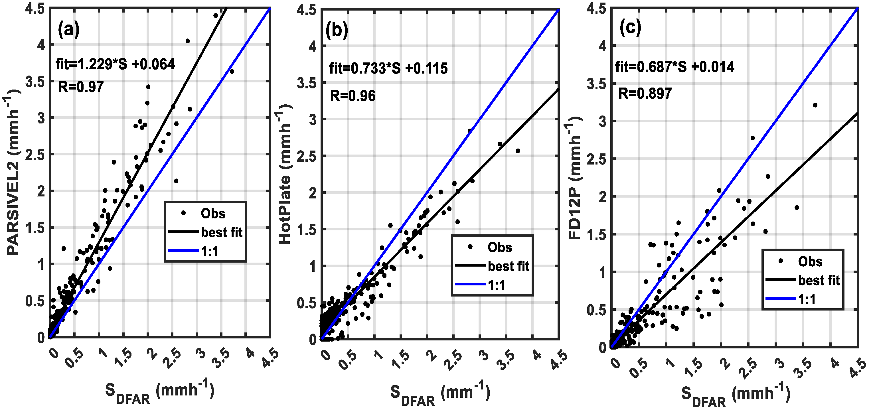
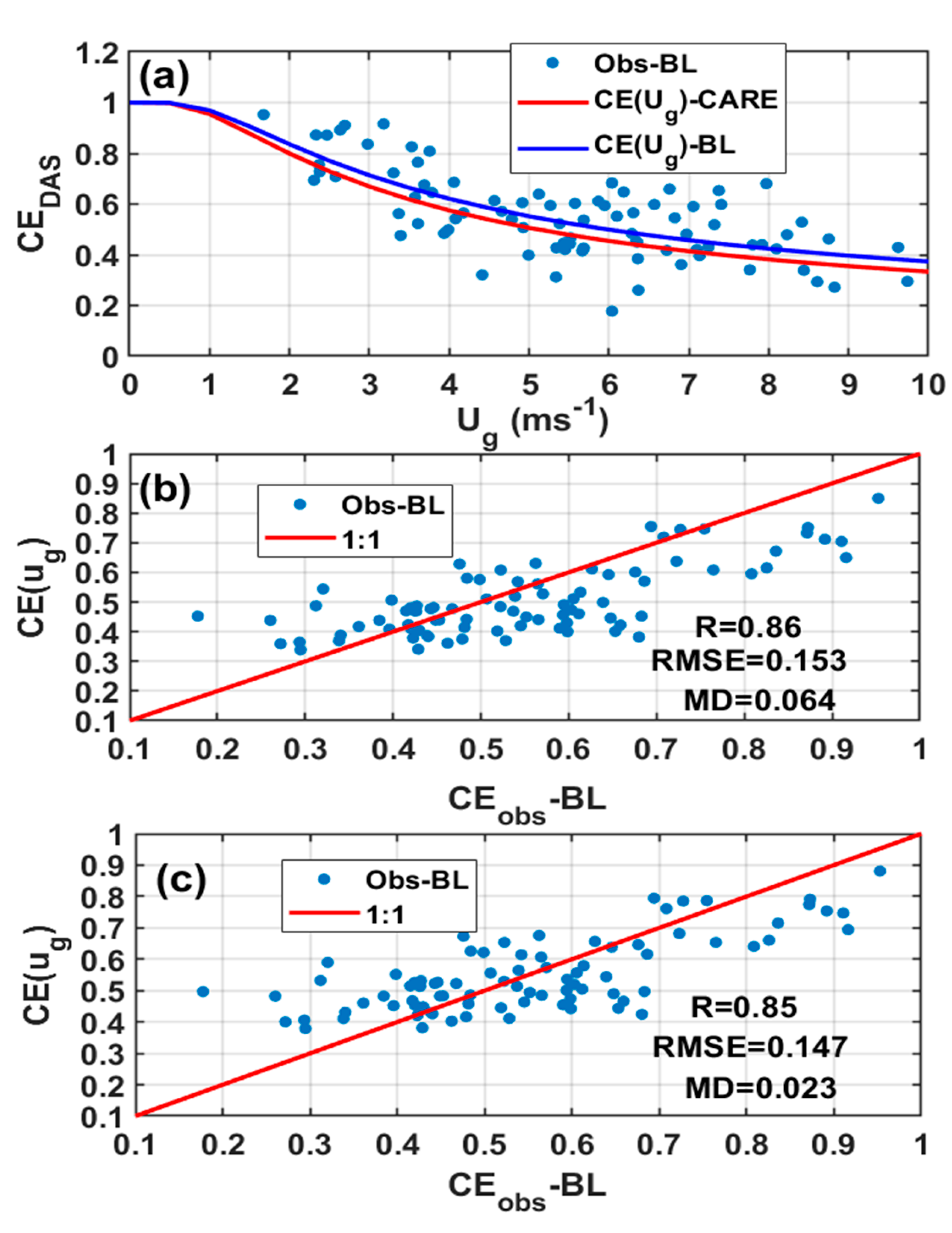
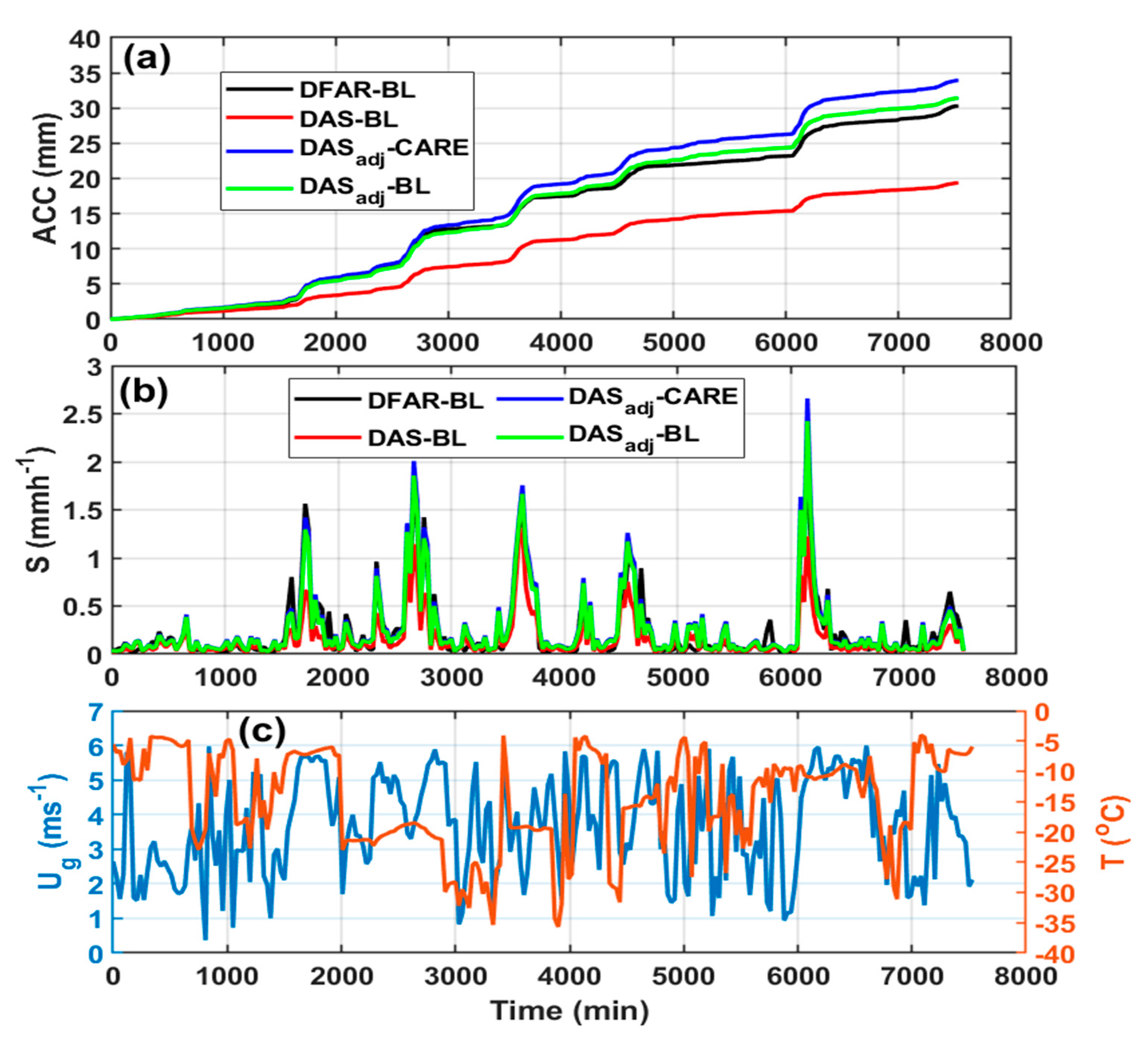
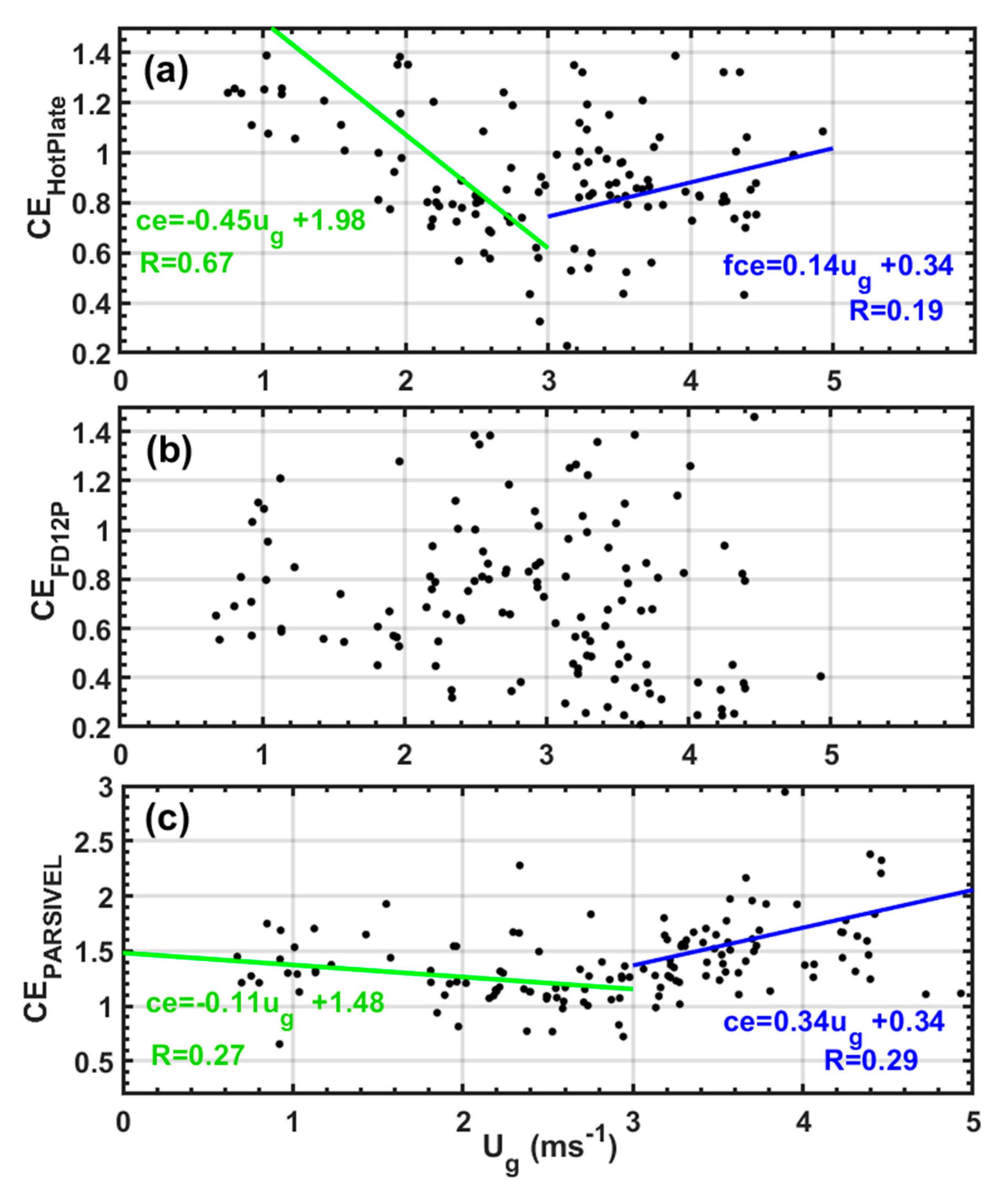
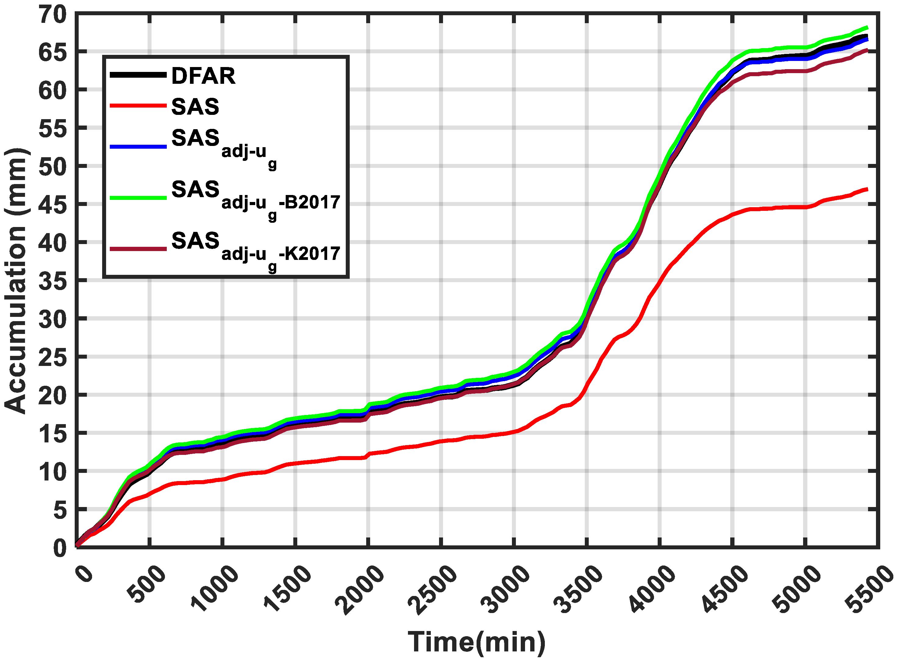
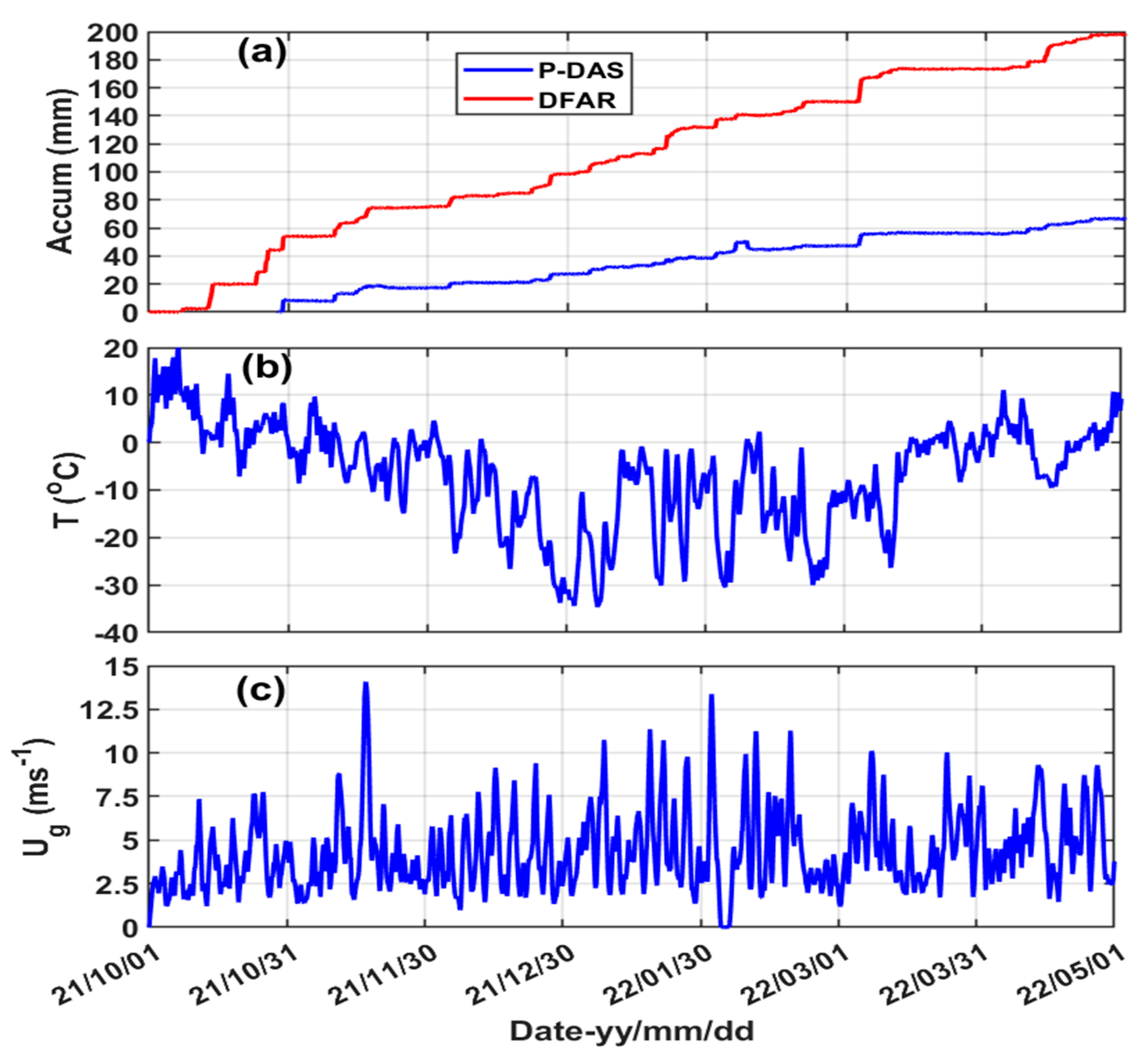
3.5. Bratt’s Lake Data

Figure 10 shows 1-min averaged precipitation accumulation based on DFAR and DAS Pluvio2 gauge (Figure 10a), temperature (Figure 10b), and gauge height wind speed (Figure 10d) observed between October 2021 and May 2022 period. During this period the precipitation accumulation (includes liquid phase) reached 200 mm according to the DFAR, but the DAS Geonor measured much less precipitation as expected partly because the gauge was active only after late October 2021. The temperature varied from 20 °C in late October 2021 to −35 °C at the end of December 2021 showing significant variability with a mean and standard deviation of −6.7 °C and 10 °C, respectively. Similarly, the wind speed varied from about 2 ms−1 to near 15 ms−1. The low wind speed (near zero) shown in February 2022 appears to be suspicious and hence have removed from the data used for this study. The mean and standard deviation of the wind speed were 4.4 m s−1and 2.7 m s−1, respectively, showing similar variability and windy conditions. Thus, it is an excellent location to test the TF of DAS gauge developed at CARE site. Unfortunately, there are no reliable disdrometer data to extract fall velocity at the site, and hence the TF that includes fall velocity cannot be evaluated.
For the collection efficiency study, from the 1-min averaged datasets shown in Figure 10, 30-min averaged data were prepared the same way as the CARE site data. In the absence of present weather sensor, the solid precipitation phase was identified based on temperature (T < −2 °C).

3.6. Comparisons of Transfer Function Based on Bratt’s Lake and CARE Data

Figure 11 shows collection efficiency of DAS Pluvio2 gauge based on the Bratts’s Lake data (Figure 11a). The transfer functions developed at CARE site and Bratt’s Lake (BL) are also shown. The new TF based on the BL data is given as
C E B L u g = 1 0.876 E x p 3.347 U g ,
As indicated in Figure 11a, the TF based on the CARE data slightly overestimated the collection efficiency. The scatter plots of the observed CE and those calculated based on TF developed using the CARE and Bratts’s Lake shown in Figure 11b,c, respectively. Based on these results, both transfer functions yield similar correlation coefficient (R = 0.85) and RMSE values (0.15), but the one based on the Bratt’s Lake gave smaller MD or mean bias value of 0.02 as compared to 0.06 which is a factor of 3 difference.
Figure 12 shows comparisons of the accumulation based on DFAR, DAS Pluvio2 (DAS), and those adjusted using the TF based on CARE data (DASadj-CARE) and based on the Bratt’s Lake (DASadj-BL) (Figure 12a), and the associated 30-min averaged S (Figure 12b) and wind speed and temperature (Figure 12c). According to these results, the DASadj-CARE slightly overestimated S by close to 12%, but the one developed based on the BL data agreed quite well. The unadjusted DAS gauge underestimates S by more than 34%. As shown in Figure 12c, the wind speed range (Ug < 6 m s−1) chosen for comparison since the TF based on CARE site data is only valid for Ug < 6 m s−1.

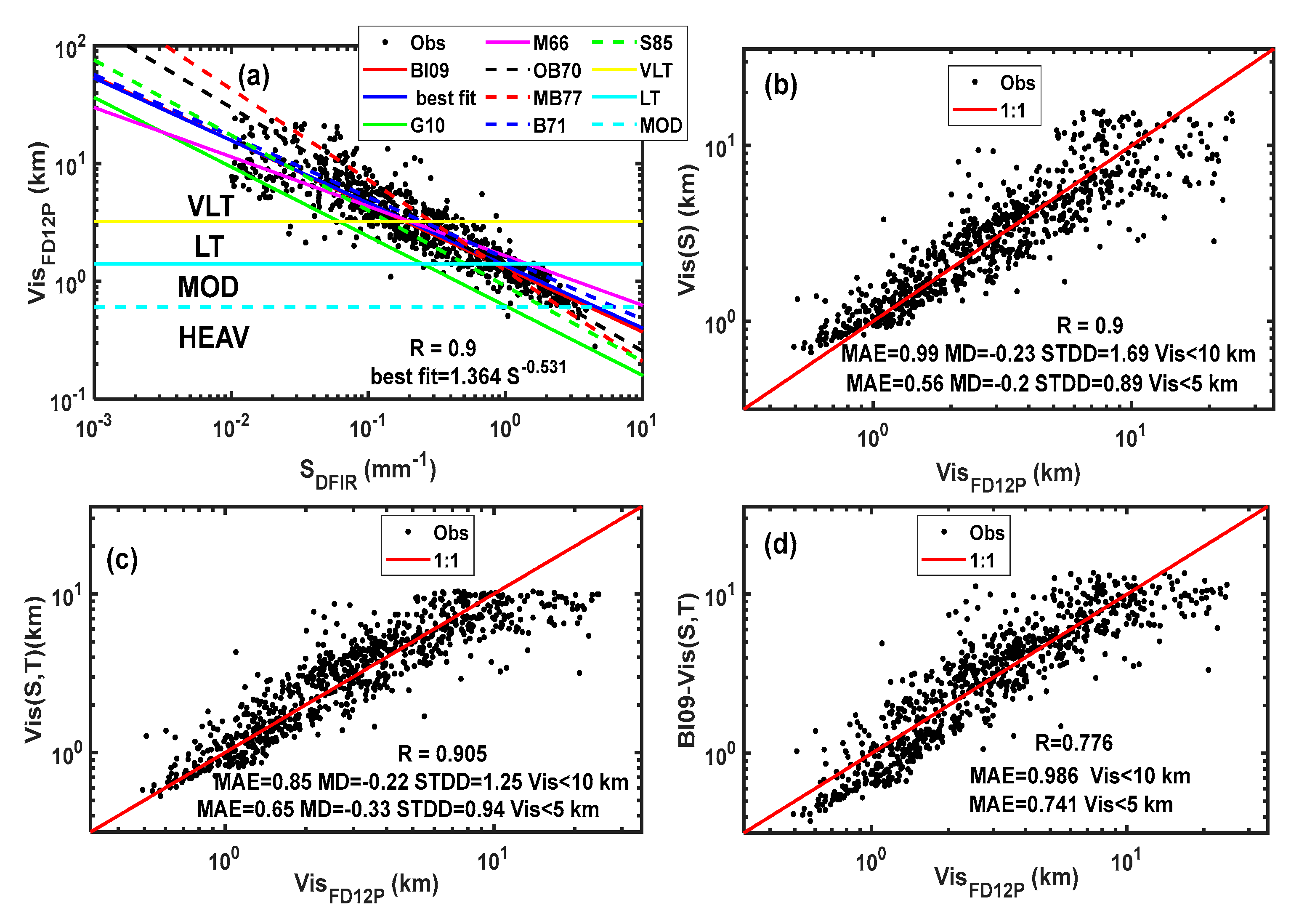
3.7. Visibility and Precipitation Intensity

Figure 13 shows 10-min averaged visibility measured using the FD12P plotted against the 10-min averaged S D F A R . According to this result, there is a tight correlation between the observed visibility and S D F A R ( R = 0.9 ) (Figure 13a), showing better agreement as compared to the previous studies that used non-standard or manually determined solid precipitation data [4,5,6]. A number of Vis parameterizations are also shown (see Table 3) as well as the Vis thresholds for solid precipitation intensity (very light (VLT), light (LT), moderate (MOD), and heavy (HEAV) based on the TC intensity thresholds as depicted in the figure. The best fit V i s ( S ) (Figure 10b), V i s ( S , T ) (Figure 10c), and based on Boudala and Isaac, (2009) ( B I 09 V i s ( S , T ) ) (Figure 10d) are also compared against observation ( V i s F D 12 P ). As indicated in Figure 13a, many of the Vis parameterizations show some discrepancies at lower visibilities (Vis < 1 km), the lower bound is based on G10 and the upper bound is based on M66. On the other hand B09 agreed well with the current parameterization (best fit) also given Figure 10b (Vis(S)). The correlation coefficient, mean absolute error (MAE), MD, and standard deviation of the difference (STDD) values calculated for Vis < 10 km and Vis < 5 km (Instrument Flight Rule (IFR) condition) for Vis(S) and Vis(S,T) are also given (Figure 10b,c). Based on these calculations, both Vis(S) and Vis(S,T) have similar MAE and MD close to 1 km and −0.2 km, respectively, indicting that both regression models overestimate Vis on average by about 0.2 km. The calculated STDD value for Vis(S) was slightly higher than the one calculated for Vis(S,T), 1.7 km and 1.3 km, respectively. For IFR conditions, the Vis(s) gives slightly better results as compared to the Vis(S,T) (Figure 13b,c). Based on visual inspection, the Vis(S,T) agrees with observation at lower Vis values better than Vis(S). The BI09-Vis(S,T) (Figure 13d) that includes temperature does not make a significant difference and generally has very similar MAE and R values of 1 km and 0.8, respectively. However when they are compared under IFR condition, BI09-Vis(S,T) has slightly higher MAE (Figure 10d).
The estimated S in m m h 1 based on Vis(S) and Vis(S,T) using the Vis thresholds adapted by the TC mentioned earlier are (0.2 < S, 0.2 < S < 1, 1 < S < 4.6, S > 4.6) and (S < 0.3, 0.3 < S < 1, 1 < S < 3.4 and S > 3.4), respectively, corresponding to VLT, LT, MOD, and HEAV intensity conditions. Both regression models gave similar results except at lower Vis where the temperature dependent version gave slightly lower intensity value. These are within the ballpark of the SAE S intensity thresholds considering the uncertainties associated with the parameterizations, particularly the one based on the Vis (S,T) except that the upper bound is overestimated by a factor of 1.36 as compared 1.84 for Vis (S). Based on physical seasoning, ref. [4] showed that under some conditions solid precipitation rate and Vis are poorly correlated, thus further studies using good quality high resolution solid precipitation data similar to the one used in this study can give better insights to reconfirm the results found in this study.

4. Conclusions

In order to contribute towards addressing some of the issues associated with solid precipitation and visibility measurements, particularly related to wind induced under or over-catchment problems of both traditional gauges and other optical probes, we have analyzed datasets collected at two sites: At the Center for Atmospheric Research experiments (CARE) and Bratt’s Lake located in southern Ontario and Saskatchewan, Canada, respectively. At the CARE site, the solid precipitation data were collected using two Geonor gauges, one placed inside a Double Fence Automated Reference (DFAR) system ( S D F A R ) and the other inside a double Alter shielded (DAS), as well as a Pluvio2 gage with a single Alter shielded configuration (SAS). The data collected at the Bratt’s Lake include a similar DFAR system and DAS Pluvio2 gauge, no present weather data are available. The solid precipitation intensity was also measured using the Yankees HotPlate, the OTT PARSIVEL2 Disdrometer, and the Vaisala FD12P present weather senor. The precipitation type and fall velocity   ( V ) were measured using the FD12P and PARSIVEL2 probes, respectively. At these sites, some auxiliary meteorological parameters such as wind speed ( U g ) and temperature (T) were also measured.
Using the data collected at CARE, we analyzed the catch efficiency (CE) of each instrument and developed a number of transfer functions as a function of U g and one other that explicitly includes V . We have tested the transfer function developed for the DAS Geonor at CARE site against the data collected at Bratt’s Lake. We have also tested two transfer functions developed based on data collected at the Marshal site in the USA ( C E R a s s 12 u g ) and eight different sites in the USA, Canada and Europe ( C E ( u g ) K 2017 ) . A new similar transfer function that is locally suitable for Bratt’s lake is also developed and tested. Using the observed visibility (Vis) and S D F A R at CARE site we have tested a number of Vis–S relationships found in the literature, and new parameterizations of visibility as a function of S and T and S lone are also developed and tested. Summary of the main findings the data analysis are given below:
Based on the data collected at CARE site, both the DAS Geonor and SAS Pluvio2 have similar catch efficiency (CE) close to 70%, but at Bratt’s Lake, the DAS Pluvio has slightly lower catch efficiency of 66%. The transfer functions developed for both DAS and SAS gauges as a function of U g at CARE site are able to adjust the solid precipitation by close to 6% and 1% difference, respectively. The transfer function developed for DAS using both U g and V performed better with no bias in the accumulation as compared to the S D F A R . The transfer function developed for SAS gauge based on data collected from the different sites in the Europe and USA ( C E ( u g ) K 2017 ) has a tendency to overestimate the CE at low and higher wind speeds ( U g > 3 ms−1), but when used for adjusting the SAS gauge, slightly underestimated the accumulation (3%). On the other hand, the TF developed for DAS gauge using the data at the Marshall site ( C E R a s s 12 u g ) in the US has a tendency to underestimate CE at low wind speeds ( U g < 3 ms−1) and adjusted the under-catch by about 8% difference.
The test performed on the DAS TF developed based on the CARE data reveals that it is well correlated (R = 0.86) with data obtained at the Bratt’s Lake data. However, the TF overestimated the snow accumulation about 12%, which is a factor of two more than when tested using the CARE datasets showing the importance of different climatology. The adjustment based on the TF developed using the Bratt’s Lake data, however, produced excellent results. We were not able to test the TF that includes fall velocity due to the lack of reliable fall velocity data.
The calculations of the CE of the solid precipitation of the non-traditional probes the FD12P, HotPlate, and PARSIVEL2 showed that the FD12P is independent of wind speed, but for the HotPlate the efficiency is decreasing and no significant systematic wind dependence for U g   < 3 ms−1 and U g   > 3 ms−1, respectively. The PARSIVEL2, however, showed some decreasing and increasing trends for wind speed ( U g   < 3 ms−1) and U g   > 3 ms−1, respectively. Generally, the solid precipitation rate measurements were correlated well with the S D F A R , but the FD12P and PARSIVEL2 underestimated and overestimated the solid precipitation by 32% and 28%, respectively. However, the HotPlate collected snow very close to the S D F A R and in this sense the HotPlate performed better than the other non-traditional optical probes with only 3.4% base as compared the DFAR measurements.
Based on this study, a tight correlation ( R = 0.9 ) was found between the observed visibility ( V i s F D 12 P ) and S D F A R and hence this has important implication for aviation application. Using the observation data S D F A R and   V i s F D 12 P , a new Vis–S relationship was derived, and the result agreed reasonably with the one given in Boudala and Isaac, (2009). The addition of temperature in visibility parameterization made no significant improvement, but the liquid water equivalent solid precipitation intensity thresholds calculated based on this equation agrees better with the one adapted by Society of Automotive Engineers.
The parameterizations developed in this study can be used for correcting solid precipitation measurements that can be applicable for validating remote sensing and NWP model data. In particular, the operationally oriented monitoring groups are now adapting the double Alter shielded gauge and hence TFs that include such as fall velocity can be useful although it may not be easily implemented for real-time applications. One of the important applications of an accurate snowfall data would be the estimation of realistic visibility, particularly for aviation applications. It should be also noted that such parameterizations, particularly the transfer functions have some limitations. As indicated in this study, although these transfer functions can be used with a reasonable accuracy when applied knowing their limitations, since they are generally site specific. Thus, when used elsewhere, they need to be used with some cautions.

Author Contributions

Project administration, funding acquisition, conceptualization, methodology, validation, formal analysis, data curation, writing—original draft preparation, F.S.B.; writing—review and editing J.A.M. All authors have read and agreed to the published version of the manuscript.

Funding

This research received no external funding.

Data Availability Statement

The data can be requested from the lead author.

Acknowledgments

The authors would like to thank Craig Smith for providing the Bratt’s Lake data, relevant information, and some valuable comments. The authors also like to thank Roy Rasmussen for his constructive comments at the earlier stage of the manuscript. The first author would like to express his deepest gratitude to Michael Di Lena, without his support this would not be possible.

Conflicts of Interest

The authors declare no conflict of interest.

Appendix A

Appendix A.1. The Description of the Geonor T-200B3

The Geonor gauge used in this study employs three transducers/wires combinations for precipitation accumulation measurements. The transducers cause the wires to vibrate, and their vibrational frequency measurements are used to determine the depth through a frequency-dependent quadratic equation, and this is converted to liquid equivalent solid precipitation.

Appendix A.2. The Description of the Pluvio2 Gauge

The Pluvio2 gauge has a sampling area of 200 cm2 and collection capacity of 1500 mm. The operating principle is based on collecting the precipitation particle in bucket and weighing the content using a high density-precision stainless steel load cell. The load cell is hermetically sealed in order to be protected from unwanted environmental effects. The sampling resolution was 6 s similar to the Geonor data. The accumulated total non-real time liquid equivalent solid precipitation was used.

Appendix A.3. The Descrption of the Vaisala FD12P Presnt Weather Senor

The Vaisala FD12P present weather sensor is an optical probe that measures precipitation intensity, precipitation type, and visibility. Its operating principle is based on forward scattering of laser light at wavelength of λ = 0.875 µm at scattering angle of 33° and also equipped with a Rain Detector (DRD12) that measures the precipitation mass. Vaisala uses a proprietary software to estimate visibility based on the observed forward scattered intensity by assuming 5% visual threshold [36]. Based on the users’ manual (https://www.manualslib.com/manual/538824/Vaisala-Fd12p.html, (accessed on 9 August 2023), the visibility is also calibrated using the Vaisala Transmissometer (Vaisala MTRAS), which operates at visible light λ = 0.550 µm. The optical precipitation intensity is estimated based on change in forward scattered light intensity and some precipitation information is also obtained from the DRD12 data. By using the fact that the optical scattering measurement is proportional to volume of falling particles and the DRD12 data are proportional to mas, ratio of the DRD12 to optical scattering data with additional temperature measurements provides the precipitation type information. The visibility is measured in range 10m–50km and the accuracy of the visibility measurements within 10 m–10 km is estimated to be ±10%, and the precipitation intensity is measured in range 0–999 mmh−1 with estimated sensitivity of 0.05 mmh−1 or less within 10 min. The accuracy of the precipitation measurements (range 0.5–20 mmh−1) is estimated to be ±30%.

Appendix A.4. The Descrption of the OTT PARSIVEL2 Disdrometer

The PARSIVEL Disdrometer measures fall velocity and size distribution of falling precipitation particles. Some descriptions of the probe can be found in the user’s manual following this link https://www.ott.com/download/operating-instructions-present-weather-sensor-ott-parsivel2-without-screen-heating-1/, (accessed on 9 August 2023). The instrument is equipped with two sensor heads, a transmitter and a receiver housed inside splash protection units. The transmitter produces 30 mm wide and 180 mm long strip of light at λ = 0.650 µm and the intensity of this light is measured by the horizontally aligned receiver. As a given precipitation particle passes through the light beam, the intensity of the light is diminished, and this is related to the particle size. The velocity of the particle is estimated using the time it takes the particle completely exit the strip of light which has about 1 mm thickness. The precipitation intensity is calculated based on velocity and size distributions, and sampling area of the probe [30,32]. The precipitation type is identified based on velocity and size measurements. In this study, no modification was applied to solid precipitation rate.

Appendix A.5. The Descrption of the HotPlate Instrument

The HotPlate instrument is interesting in sense that the precipitation intensity can be calculated directly using the first principle of heat transfer [33,34]. This is achieved by using two identical circular aluminum plates are vertically stacked together exposing the area of upper plate to falling particle while the lower plate is facing downward is sheltered from falling particles. The dimeter of these plates is 13 cm and there are smaller concentric circle within inside the bigger circle to help prevent falling particles from sliding off of the upper plate. Both plates are heated to the same temperature of about 75 °C, but the plates are insulated so that no heat transfers between them. In the absence of precipitation, both plates cool due to forced convection, and hence the difference is expected to be near zero. Under precipitation, the difference in cooling rate between the two plates can be related to precipitation rate. As discussed in [33] the major problems associated with the HotPlate instrument are the effect of wind and false precipitation because of imbalance in forced convection of the two plates under clear conditions. The detailed description of the heat transfer equations and associated correction factors are given in [33]. All the optically based instruments and the HotPlate have been set to collect data at 1 min temporal resolution.

References

  1. Ballesteros, J.A.A.; Hitchens, N.M. Meteorological Factors Affecting Airport Operations during the Winter Season in the Midwest. Weather. Clim. Soc. 2018, 10, 307–322. [Google Scholar] [CrossRef]
  2. Das, S.; Brimley, K.B.; Lindheimer, E.T.; Zupancich, M. Association of reduced visibility with crash outcomes. IATSS Res. 2018, 42, 143–151. [Google Scholar] [CrossRef]
  3. Eisenberg, D.; Warner, E.K. Effects of Solid precipitations on Motor Vehicle Collisions, Injuries, and Fatalities. Am. J. Public Health 2005, 95, 120–124. [Google Scholar] [CrossRef] [PubMed]
  4. Rasmussen, R.M.; Vivekanandan, J.; Cole, J.; Myers, B.; Masters, C. The estimation of solid precipitation rate using visibility. J. Appl. Meteor. 1999, 38, 1542–1563. [Google Scholar] [CrossRef]
  5. Boudala, F.S.; Isaac, G.A. Parameterization of visibility in snow: Application in numerical weather prediction models. J. Geophys. Res. 2009, 114, D19202. [Google Scholar] [CrossRef]
  6. Gultepe, I.; Milbrandt, J.; Zhou, B.-B. Visibility parameterization for forecasting model applications. In Proceedings of the 5th International Conference onFog, Fog Collection and Dew, Münster, Germany, 25–30 July 2010; pp. 227–230. [Google Scholar]
  7. Falconi, M.T.; von Lerber, A.; Ori, D.; Marzano, F.S.; Moisseev, D. Solid precipitation retrieval at X, Ka and W bands: Consistency of backscattering and microphysical properties using BAECC ground-based measurements. Atmos. Meas. Tech. 2018, 11, 3059–3079. [Google Scholar] [CrossRef]
  8. Goodison, B.E.; Louie, P.Y.T.; Yang, D. WMO Solid Precipitation Measurement Intercomparison. In World Meteorological Organization, Instruments and Observing Methods; Report No. 67, WMO/TD—No. 872; 1998; 88p. Available online: https://library.wmo.int/doc_num.php?explnum_id=9694 (accessed on 9 August 2023).
  9. Goodison, B.E.; Yang, D. In-situ measurement of solid precipitation in high latitudes: The need for correction. In Proceedings of the ACSYS Solid Precipitation Climatology Project Workshop, Reston, VA, USA, 12–15 September 1995; WMO/TD- No.739, WMO, 1–12. Available online: https://library.wmo.int/doc_num.php?explnum_id=9637 (accessed on 9 August 2023).
  10. Kochendorfer, J.; Nitu, R.; Wolffm, M.; Mekis, E.; Rasmussen, R.; Baker, B.; Earle, M.E.; Reverdin, A.; Wong, K.; Smith, C.; et al. Analysis of single- Alter-shielded and unshielded measurements of mixed and solid precipitation from WMO-SPICE. Hydrol. Earth Syst. Sci. 2017, 21, 3525–3542. [Google Scholar] [CrossRef]
  11. Kochendorfer, J.; Rasmussen, R.; Wolff, M.; Baker, B.; Hall, M.E.; Meyers, T.; Landolt, S.; Jachcik, A.; Isaksen, K.; Brækkan, R.; et al. The quantification and correction of windinduced precipitation measurement errors. Hydrol. Earth Syst. Sci. 2017, 21, 1973–1989. [Google Scholar] [CrossRef]
  12. Kochendorfer, J.; Earle, M.; Rasmussen, R.; Smith, C.; Yang, D.; Morin, S.; Mekis, E.; Buisan, S.; Roulet, Y.-A.; Landolt, S.; et al. How well are we measuring snow post-SPICE. Am. Meteorol. Soc. 2022, 103, 370–378. [Google Scholar] [CrossRef]
  13. Smith, C.D.; Yang, D. An assessment of the Geonor T-200B used with a large octagonal double fence wind shield as an automated reference for the gauge measurement of solid precipitation. In Proceedings of the 90th AMS Annual Meeting/15th SMOI, Atlanta, GA, USA, 16–21 January 2010; Available online: https://ams.confex.com/ams/pdfpapers/158669.pdf (accessed on 9 August 2023).
  14. Pierre, A.; Jutras, S.; Kochendorfer, J.; Smith, C.; Fortin, V.; Anctil, F. Evaluation of catch efficiency transfer functions for unshielded and single-Alter-shielded solid precipitation measurements. J. Atmos. Ocean. Technol. 2019, 36, 865–881. [Google Scholar] [CrossRef]
  15. Køltzow, M.; Casati, B.; Haiden, T.; Valkonen, T. Verification of Solid Precipitation Forecasts from Numerical Weather Prediction Models in Norway. Wea. Forecasting. 2020, 35, 2279–2292. [Google Scholar] [CrossRef]
  16. Kochendorfer, J.; Nitu, R.; Wolff, M.; Mekis, E.; Rasmussen, R.; Baker, B.; Earle, M.E.; Reverdin, A.; Wong, K.; Smith, C.D.; et al. Testing and development of transfer functions for weighing precipitation gauges in WMO-SPICE, Hydrol. Earth Syst. Sci. 2020, 22, 1437–1452. [Google Scholar] [CrossRef]
  17. Wolff, M.A.; Isaksen, K.; Petersen-Øverleir, A.; Ødemark, K.; Reitan, T.; Brækkan, R. Derivation of a new continuous adjustment function for correcting wind-induced loss of solid precipitation: Results of a Norwegian field study. Hydrol. Earth Syst. Sci. 2015, 19, 951–967. [Google Scholar] [CrossRef]
  18. Colli, M.; Stagnaro, M.; Lanza, L.G.; Rasmussen, R.; Thériault, J.M. Adjustments for Wind-Induced Undercatch in Snowfall Measurements Based on Precipitation Intensity. J. Hydrometeorol. 2020, 21, 1039–1050. [Google Scholar] [CrossRef]
  19. Rasmussen, R.M.; Baker, B.; Kochendorfer, J.; Meyers, T.; Landolt, S.; Fischer, A.P.; Black, J.; Thériault, J.M.; Kucera, P.; Gochis, D.; et al. How well are we measuring snow: The NOAA/FAA/NCAR winter precipitation test bed. Bull. Amer. Meteor. Soc. 2012, 93, 811–829. [Google Scholar] [CrossRef]
  20. Leroux, N.R.; Thériault, J.M.; Rasmussen, R. Improvement of snow gauge collection efficiency through a knowledge of solid precipitation fall speed. J. Hydrometeor. 2021, 22, 997–1006. [Google Scholar] [CrossRef]
  21. Hoover, J.; Earle, M.E.; Joe, P.I.; Sullivan, P.E. Unshielded precipitation gauge collection efficiency with wind speed and hydrometeor fall velocity. Hydrol. Earth Syst. Sci. 2021, 25, 5473–5491. [Google Scholar] [CrossRef]
  22. Thériault, J.M.; Rasmussen, R.; Ikeda, K.; Landolt, S. Dependence of snow gauge collection efficiency on snowflake characteristics. J. Appl. Meteor. Climatol. 2012, 51, 745–762. [Google Scholar] [CrossRef]
  23. Smith, C.D.; Yang, D.; Ross, A.; Barr, A. The Environment and Climate Change Canada solid precipitation intercomparison data from Bratt’s Lake and Caribou Creek, Saskatchewan. Earth Syst. Sci. 2019, 11, 1337–1347. [Google Scholar] [CrossRef]
  24. Nitu, R.; Roulet, Y.-A.; Wolff, M.; Earle, M.; Reverdin, A.; Smith, C.; Kochendorfer, J.; Morin, S.; Rasmussen, R.; Wong, K.; et al. WMO Solid Precipitation Intercomparison Experiment (SPICE) (2012–2015); Instruments and Observing Methods Report No. 131; World Meteorological Organization: Geneva, Switzerland, 2018. [Google Scholar]
  25. Smith, C.D.; Ross, A.; Kochendorfer, J.; Earle, M.E.; Wolff, M.; Buisán, S.; Roulet, Y.-A.; Laine, T. Evaluation of the WMO Solid Precipitation Intercomparison Experiment (SPICE) transfer functions for adjusting the wind bias in solid precipitation measurements. Hydrol. Earth Syst. Sci. 2020, 24, 4025–4043. [Google Scholar] [CrossRef]
  26. Nitu, R. Proposed configuration of intercomparison sites and of the field references. In Second Session of the International Organization Committee for the WMO Solid Precipitation Intercomparison Experiment; World Meteorological Organization: Boulder, CO, USA, 2012. [Google Scholar]
  27. Boudala, F.S.; Hudak, D.; Boodoo, S.; Donaldson, N.; Nitu, R.; Wong, K. Improved Algorithms for Radar Remote Sensing of Solid precipitation Rate Using Dual Polarization C Band Radar. In Proceedings of the 17th International Conference on Clouds and Precipitation, ICCP 2016, Manchester, UK, 25–29 July 2016. [Google Scholar]
  28. Boudala, F.S.; Isaac, G.A.; Filman, P.; Crawford, R.; Hudak, D. Performance of Emerging Technologies for Measuring Solid and Liquid Precipitation in Cold Climate as Compared to the Traditional Manual Gauges. J. Atmos. Oceanic Technol. 2017, 34, 167–184. [Google Scholar] [CrossRef]
  29. Haavasoja, T.; Nnqvist, J.L.; Nylander, P. ‘Present Weather and Fog Detection for Highways. In Proceedings of the Seventh Road Conference, Seefeld, Austria, 21–22 March 1994. [Google Scholar]
  30. Loffler-Mang, M.; Joss, J. An optical Disdrometer for measuring size and velocity of hydrometeors. J. Atmos. Oceanic Technol. 2000, 17, 130–139. [Google Scholar] [CrossRef]
  31. Battaglia, A.; Rustemeier, E.; Tokay, A.; Blahak, U.; Simmer, C. Parsivel snow observations: A critical assessment. J. Atmos. Ocean. Tech. 2010, 27, 333–344. [Google Scholar] [CrossRef]
  32. Boudala, F.S.; Isaac, G.A.; Rasmussen, R.; Cober, S.; Scott, B. Comparisons of snowfall measurements in complex terrain made during the 2010 Winter Olympics in Vancouver. Pure Appl. Geophys. 2014, 171, 113. [Google Scholar] [CrossRef]
  33. Boudala, F.S.; Rasmussen, R.; Isaac, G.A.; Scott, B. Performance of hot plate for measuring solid precipitation in complex terrain during the 2010 Vancouver Winter Olympics. J. Atmos. Oceanic Technol. 2014, 31, 437–446. [Google Scholar] [CrossRef]
  34. Rasmussen, R.M.; Hallett, J.; Purcell, R.R.; Landolt, S.D.; Cole, J. The hotplate precipitation gauge. J. Atmos. Oceanic Technol. 2011, 28, 148–164. [Google Scholar] [CrossRef]
  35. Transport Canada (TC), 2020–2021. Transport Canada Holdover Time (HOT) Guidelines Winter 2020–2021. Available online: https://tc.canada.ca/en/aviation/general-operating-flight-rules/holdover-time-hot-guidelines-icing-anti-icing-aircraft (accessed on 9 August 2023).
  36. Boudala, F.S.; Isaac, G.A.; Crawford, R.; Reid, J. Parameterization of runway visual range as a function of visibility: Application in in numerical weather prediction models. J. Atmos. Ocean. Technol. 2012, 29, 177–191. [Google Scholar] [CrossRef]
  37. Boudala, F.S.; Wu, D.; Isaac, G.A.; Gultepe, I. Seasonal and Microphysical Characteristics of Fog at a Northern Airport in Alberta, Canada. Remote Sens. 2022, 14, 4865. [Google Scholar] [CrossRef]
  38. Leroux, 2022. Guide to Aircraft Deicing. Available online: https://www.sae.org/works/committeeResources.do?resourceID=900393 (accessed on 9 August 2023).
  39. Mitchell, D.L. Use of mass- and area-dimensional power laws for determining precipitation particle terminal velocities. J. Atmos. Sci. 1996, 53, 1710–1723. [Google Scholar] [CrossRef]
  40. Thériault, J.M.; Rasmussen, R.; Petro, E.; Colli, M.; Lanza, L. Impact of wind direction, wind speed and particle characteristics on the collection efficiency of the Double Fence Intercomparison. J. Appl. Met. Clim. 2015, 54, 1918–1930. [Google Scholar] [CrossRef]
  41. Mellor, M. Light scattering and particle aggregation in snow-storms. J. Glaciol. 1966, 6, 237–248. [Google Scholar] [CrossRef]
  42. Warner, C.; Gunn, K.L.S. Measurement of solid precipitation by optical attenuation. J. Appl. Meteorol. 1969, 8, 110–121. [Google Scholar] [CrossRef]
  43. O’Brien, H.W. Visibility and light attenuation in falling snow. J. Appl. Meteorol. 1970, 9, 671–683. [Google Scholar] [CrossRef]
  44. Stallabrass, J.R. Measurements of the concentration of falling snow. Tech. Memo. 140. In Proceedings of the Snow Property Measurements Workshop, Lake Louise, AB, Canada, 1–3 April 1985. [Google Scholar]
  45. Fujiyoshi, Y.; Wakahamam, G.; Endoh, T.; Irikawa, S.; Konishi, H.; Takeuchi, M. Simultaneous observation of solid precipitation intensity and visibility in winter at Saporro. Low Temp. Sci. 1983, 42A, 147–156. [Google Scholar]
  46. Bisyarin, V.P.; Bisyarina, I.P.; Rubash, V.K.; Sokolov, A.K. Attenuation of 10.6 and 0.63 mm laser radiation in atmospheric precipitation. Radio Eng. Electron. Phys. 1971, 16, 1594. [Google Scholar]
  47. Muench, H.S.; Brown, H.A. Measurement of Visibility and Radar Reflectivity during Snowstorms in the AFGL Mesonet; Project 8628; 1977. Available online: https://apps.dtic.mil/sti/citations/ADA049258 (accessed on 15 May 2023).
Figure 1. The configuration of the DFAR (a), a single Alter shielded Geonor inside an orthogonal shield (b) and double Alter shielded Geonor (c).
Remotesensing 15 04079 g001
Figure 2. Precipitation type represented by symbols (C = clear, snow, S = snow, SP = snow pellets, IP = ice pellets, snow grain = SG, IC = ice crystal, R = rain, L = Drizzle, P = unknown, M = mixed phase, ZL = freezing drizzle, and ZR = freezing rain, (a), temperature (b), and 10 min averaged wind speed ( U G ) (c) and 1 min averaged maximum wind measured at 3 m height (d).
Remotesensing 15 04079 g002
Figure 3. The frequency distribution of fall velocity ( V ) of snow (a), snow grain (b), ice crystals (c), and drizzle (d) based on the PARSIVEL2 data.
Remotesensing 15 04079 g003
Figure 4. Collection efficiency (CE) of Geonor with double Alter shield as a function of gauge height wind speed ( U g ) and fall velocity (V) (a), comparisons of the parameterization of CE as a function of U g (b), based on [19] (Rass12) (c) and as a function of U g and V (d) against observation. The Root Mean Square Errors (RMSE) and the mean difference (MD) or mean bias values are also indicated.
Remotesensing 15 04079 g004
Figure 5. Collection efficiency of HotPlate (a), FD12P (b), and PARSIVEL2 (c) as a function of wind speed ( U g ) measured at gauge height level (c). Linearly fitted CE lines for HotPlate and PARSIVEL are also given.
Remotesensing 15 04079 g005
Figure 6. Comparisons of the solid precipitation S D F I R and PARSIVEL2 (a), HotPlate (b), and FD12P (c).
Remotesensing 15 04079 g006
Figure 7. Comparisons of snow accumulation of SDFAR, and several instruments given in Figure 6, unadjusted ( D A S ), adjusted (adj) based on the transfer functions in Table 1 ( D A S u g ), ( D A S u g v ), and ( D A S u g r a s s 12 ) (a) and the associated solid precipitation intensities (b).
Remotesensing 15 04079 g007
Figure 8. Collection efficiency of Pluvio2 with a single Alter shield ( C E P l u v i o 2 ) (a), the observed ( C E o b s ) compared to C E u g (b), C E ( u g ) B 2017 , [28] (c) and C E ( u g ) K 2017 [10] (d). The RMSE and MD or mean bias values are also indicated.
Remotesensing 15 04079 g008
Figure 9. Accumulation of S based on the S D F A R , adjusted (adj) with C E u g ( S A S u g ) , C E u g B 2017 ( S A S u g B 0217 ) , and C E u g K 2017 ( S A S u g K 2027 ) .
Remotesensing 15 04079 g009
Figure 10. The precipitation based on double Alter shielded Pluvio2 gauge (P-DAS) and DFAR (a), temperature (T) (b) and wind speed ( U g ) (c) observed in Baratt’s Lake site.
Remotesensing 15 04079 g010
Figure 11. The observed collection efficiency (CE) of DAS Pluvio2 ( C E u g D A S ) and the transfer functions based on Bratt’s Lake (BL) and CARE site (a), comparisons of the observed collection efficiency in BL ( C E o b s B L ) and CE-based TF at CARE site (b) and based on BL (c). The RMSE and MD or mean bias values are also given.
Remotesensing 15 04079 g011
Figure 12. The observed solid precipitation accumulation in Bratt’s Lake based on the DFAR (DFAR-BL) and DAS-BL Pluvio2 gauge, and the adjusted DAS using the CARE TF (DASadj-CARE) and based on BL TF (DASadj-BL) (a), and associated 30 min averaged precipitation intensity (b), and wind speed (Ug) and temperature (T) (c).
Remotesensing 15 04079 g012
Figure 13. Comparisons of visibility measured using the FD12P ( V i s F D 12 P ) and S D F I R , a number of parameterizations in Table 2 of (a), the best fit lines V i s ( S ) (b) and V i s ( S , T ) (c), and based on [5] (d). Water equivalent solid precipitation intensity thresholds very light (VLT), light (LT), moderate (MOD), and heavy (HEAV) based on visibility adapted by Transport Canada are shown including the calculated MAE, MD, and STDD.
Remotesensing 15 04079 g013
Table 1. Transfer functions for collection efficiency of double Alter shielded Geonor gauge.
SourcesCatch Efficiency ParameterizationRMSE
In this work-Geonor double Alter shield, at CARE site C E u g = 1 0.9 exp ( 3 U g ) 0.074
In this work at CARE site C E u g , v = exp ( 0.0233 U g 2.275 + 0.3553 V 0.4483 ) 0.07
Rasmussen et al., 2012 based on data at Marshall site, USA [19] C E R a s s 12 u g = 0.94 0.09 U g 0.09
Table 2. Transfer functions for collection efficiency (CE) for single Alter shield Pluvio2.
SourcesCatch Efficiency ParameterizationRMSE
In this work at CARE site C E u g = 1 1.522 exp ( 4.758 U g ) 0.13
Boudala et al., (2017) in Cold Lake Alberta [28] C E B 17 u g = 1 1.517 exp ( 4.595 U g ) 0.13
Kochendorfer et al., (2017a) [10]
Based on 8 different sites
C E B 17 u g = 0.336 + 0.728 exp ( 0.23 U g ) 0.14
Table 3. Visibility parameterizations based on solid precipitation.
SourceParameterization
This work -Vis(S) exp ( 0.31 0.531 l n ( S ) )
Boudala and Isaac, 2009 (BI09(S)) [5] exp ( 0.3 0.547 l n ( S ) )
This work -Vis(S,T) exp ( 0.33 + 0.0034 T 0.678 ln S + 0.04 )
Boudala and Isaac, 2009 (BI09(S,T) [5] exp ( 0.399 + 0.0288 T 0.783 ln S + 0.04 )
Mellor (1966) (M66) [41] exp ( 0.501 0.42 ln S )
Warner and Gunn (1969) [42] exp ( 0.432 l n ( S ) )
O’Brien (1970) (OB70) [43] exp ( 0.223 0.69 l n ( S ) )
Gultepe et al. (2010) (G10) [44] exp ( 0.478 0.59 ln S )
Stallabrass (1985) (S85) exp ( 0.089 0.64 ln S )
Fujiyoshi et al. (1983) [45] exp ( 0.66 ln S )
Bisyarin et al. (1971) (B71) [46] exp ( 0.451 0.52 ln S )
Muench and Brown (1977) (MB77) [47] exp ( 0.215 0.77 ln S )
Disclaimer/Publisher’s Note: The statements, opinions and data contained in all publications are solely those of the individual author(s) and contributor(s) and not of MDPI and/or the editor(s). MDPI and/or the editor(s) disclaim responsibility for any injury to people or property resulting from any ideas, methods, instructions or products referred to in the content.

