Article

Robust Dual Spatial Weighted Sparse Unmixing for Remotely Sensed Hyperspectral Imagery

1
Jiangxi Province Key Laboratory of Water Information Cooperative Sensing and Intelligent Processing, School of Information Engineering, Nanchang Institute of Technology, Nanchang 330099, China
2
Guangzhou Institute of Building Science Group Co., Ltd., Guangzhou 510440, China
*
Author to whom correspondence should be addressed.
Remote Sens. 2023, 15(16), 4056; https://doi.org/10.3390/rs15164056
Submission received: 22 June 2023 / Revised: 7 August 2023 / Accepted: 12 August 2023 / Published: 16 August 2023
(This article belongs to the Special Issue Spectral Unmixing of Hyperspectral Remote Sensing Imagery II)

Abstract

:
Sparse unmixing plays a crucial role in the field of hyperspectral image unmixing technology, leveraging the availability of pre-existing endmember spectral libraries. In recent years, there has been a growing trend in incorporating spatial information from hyperspectral images into sparse unmixing models. There is a strong spatial correlation between pixels in hyperspectral images (that is, the spatial information is very rich), and many sparse unmixing algorithms take advantage of this to improve the sparse unmixing effect. Since hyperspectral images are susceptible to noise, the feature separability of ground objects is reduced, which makes most sparse unmixing methods and models face the risk of degradation or even failure. To address this challenge, a novel robust dual spatial weighted sparse unmixing algorithm (RDSWSU) has been proposed for hyperspectral image unmixing. This algorithm effectively utilizes the spatial information present in the hyperspectral images to mitigate the impact of noise during the unmixing process. For the proposed RDSWSU algorithm, which is based on 1 sparse unmixing framework, a pre-calculated superpixel spatial weighting factor is used to smooth the noise, so as to maintain the original spatial structure of hyperspectral images. The RDSWSU algorithm, which builds upon the 1 sparse unmixing framework, employs a pre-calculated spatial weighting factor at the superpixel level. This factor aids in noise smoothing and helps preserve the inherent spatial structure of hyperspectral images throughout the unmixing process. Additionally, another spatial weighting factor is utilized in the RDSWSU algorithm to capture the local smoothness of abundance maps at the sub-region level. This factor helps enhance the representation of piecewise smooth variations within different regions of the hyperspectral image. Specifically, the combination of these two spatial weighting factors in the RDSWSU algorithm results in an enhanced sparsity of the abundance matrix. The RDSWSU algorithm, which is a sparse unmixing model, offers an effective solution using the alternating direction method of multiplier (ADMM) with reduced requirements for tuning the regularization parameter. The proposed RDSWSU method outperforms other advanced sparse unmixing algorithms in terms of unmixing performance, as demonstrated by the experimental results on synthetic and real hyperspectral datasets.

1. Introduction

Hyperspectral imaging spectrometers have the ability to capture images of specific regions in the electromagnetic spectrum, enabling the detection of objects that are unidentifiable in wide-band imaging remote sensing [1]. The use of hyperspectral remote sensing images enables the acquisition of data containing abundant information about the Earth surface, thereby providing the potential for achieving quantitative and refined ground observation [2]. Hyperspectral remote sensing imagery has been widely utilized in diverse fields, encompassing marine exploration [3], environmental monitoring [4], forestry monitoring [5], geological exploration [6], modern military affairs [7], and precision agriculture [4]. Owing to the limited spatial resolution of imaging sensors and the intricate variability of ground features, hyperspectral remote sensing images often exhibit mixed pixels. This phenomenon poses challenges in accurately interpreting the information related to ground objects. This seriously restricts the development and application of quantitative analysis in hyperspectral remote sensing [8]. To cope with the problem of mixed pixels, spectral unmixing [9] techniques have been introduced to effectively identify the spectral characteristics of different ground features in each pixel, called endmembers, and estimate their corresponding percentages, called abundance. This is a key method for analyzing hyperspectral images.
The linear mixture model (LMM) becomes an active research line in hyperspectral imaging analysis owing to its simplicity and mathematical tractability [10]. LMM assumes that the spectral signature of a mixed pixel can be represented as a linear combination of the spectra of multiple endmembers. Building upon LMM, various unsupervised spectral unmixing methods have been developed, including geometry-based approaches [11,12,13] and statistics-based approaches [14,15]. However, most of these methods require extracting endmembers directly from the given scene, which can lead to obtaining virtual endmembers that have no physical meaning from mixed hyperspectral images [16]. Sparse unmixing methods have emerged as a solution to tackle this issue [17,18,19]. These methods adopt a semi-supervised approach, aiming to identify the optimal subset of entries from a known endmember spectral library that effectively represents the mixed pixels in a hyperspectral image. By leveraging sparsity constraints, they seek to achieve a sparse representation of the mixed pixels using a reduced set of endmembers [20,21].
In the context of sparse unmixing, the abundance vector associated with a mixed pixel is characterized by containing far fewer elements than the total number of spectral signatures present in a given spectral library. As a result, the abundance vector exhibits sparsity as a prominent feature [22]. To enhance the sparsity of solutions, several typical methods have been proposed. For example, the renowned SUnSAL [17] algorithm utilizes the 1 regularizer to promote sparsity in the fractional abundances, yielding promising outcomes. Moreover, the collaborative SUnSAL algorithm, known as CLSUnSAL [23], incorporates the 2 , 1 regularizer to leverage collaborative row sparsity across all pixels. In order to further punish the abundance coefficient, some studies introduce the weight factor into the sparse unmixing models [24,25,26]. The DRSU [27] algorithm employs dual weight factors to efficiently boost the sparsity of the fractional abundance. While the aforementioned sparse unmixing algorithms demonstrate promising potential, they primarily emphasize the utilization of spectral information from hyperspectral images while overlooking the incorporation of spatial information, which impacts the accuracy of unmixing.
Spatial-contextual information is a valuable resource that can be harnessed to enhance the effectiveness of unmixing techniques in practical applications [28]. The incorporation of spatial information into sparse unmixing models has become a prominent approach, leading to the development of numerous sparse unmixing algorithms that leverage spatial information. For example, the SUnSAL-TV [29] algorithm utilizes anisotropic total variation regularization to encourage the smoothing of spatial neighborhoods in images. The NLSU [30] algorithm utilizes a non-local spatial regularization technique to identify and capture resemblances in patterns and structures present in the abundance map. Furthermore, a S 2 WSU method is introduced, incorporating spectral and spatial weight factors to enhance the sparsity of solutions within the 1 sparse regularization framework. The proposed DRSU-TV [31] method is developed, which utilizes a combination of double weighted factors and TV regularization to improve the sparsity of solutions while simultaneously achieving smoothness in the abundance map. A novel approach, based on superpixels and graph regularization, has been proposed for sparse unmixing [32]. This method leverages spectral weighting factors to encourage sparsity in the solutions, while utilizing a graph regularization term to enhance the spatial correlation of the resulting images. These methods can enhance the accuracy of abundance estimation to a certain degree. Nevertheless, in scenarios where hyperspectral images are heavily corrupted by high levels of noise, these methods often struggle and achieving satisfactory accuracy in unmixing becomes challenging. For this problem, a self-supervised robust deep unmixing model (SSRDMF) is presented [33], which decreases the influence of Gaussian noise and sparse noise through the deep autoencoder, thereby enhancing unmixing capabilities. The spectral-spatial robust NMF unmixing model (SSRNMF) is introduced [34], leveraging double regularization norms to attain noise robustness, resulting in favorable outcomes. The SSNPNMF unmixing model [35] is presented, building a graph based on spatial-spectral information to modify the reconstruction weight values of pixels and neighboring pixels, mitigating noise effects.
In recent years, superpixel segmentation technology has gained widespread adoption in the field of hyperspectral image processing due to its effectiveness in enhancing data interpretation performance [36], such as hyperspectral image classification [37,38], spectral unmixing [39], denoising [40], fusion [41] and other fields. For example, a superpixel-based weighting method was proposed in [42] to exploit the spatial correlation of images. In [43], a sparse unmixing model incorporating superpixel reweighted low-rank constraint and TV regularization is introduced, aiming to promote the smoothness of the image.
In order to effectively deal with spectral unmixing task under low signal-to-noise ratio (SNR) [44], in view of the advantages of superpixel segmentation strategy, a novel robust dual spatial weighted sparse unmixing (RDSWSU) algorithm is proposed in this paper. The main objective of the proposed RDSWSU algorithm is to acquire more precise spatial context information in order to mitigate the adverse impact of noise on the unmixing process. Specifically, for the proposed RDSWSU algorithm, which is based on the 1 sparse regularization framework, on the one hand, the pre-calculated spatial weighting factor based on superpixel is used to smooth the noise. On the other hand, the utilization of a spatial weighting factor enhances the spatial coherence of the abundance map.
The efficient solution to the optimization problem of the proposed RDSWSU algorithm can be achieved by leveraging the ADMM technique [45]. To sum up, we can summarize the contribution of this paper. For the newly proposed RDSWSU method, based on the 1 sparse unmixing framework, it introduced two key enhancements: the utilization of pre-calculated superpixel spatial weighting factor and spatial neighborhood weighting factor. These improvements aimed to reduce the impact of noise on unmixing and capture the localized smoothness characteristics of the abundance map, respectively. The RDSWSU unmixing model, as proposed, demonstrates a notable enhancement in its ability to handle high levels of noise in challenging scenes. Furthermore, it effectively preserves the precise spatial information of images, thereby leading to improved accuracy in the unmixing process. Moreover, our proposed model has a simple formulation with only one regularization parameter, which makes it easy to tune.
The remaining sections of the paper are outlined as follows. Section 2 is dedicated to the introduction of the linear spectral unmixing model. In Section 3, a detailed description of our proposed robust dual spatial weighted sparse unmixing model is provided. Section 4 specifically presents the experimental results using synthetic hyperspectral data, whereas Section 5 focuses on showcasing experimental results using actual hyperspectral data. Finally, Section 6 concludes the paper by providing a summary, remarks, and suggestions for future research topics.

2. Linear Spectral Unmixing

Suppose we have an observed hyperspectral image denoted by Y R L × n , where n represents the total number of pixel vectors and L represents the number of spectral bands. Let A R L × m be a comprehensive spectral library comprising m spectral signatures. The aim of sparse unmixing is to identify the most suitable subset of endmembers from the spectral library A in order to represent mixed pixels in a hyperspectral image. To sum up, the LMM can be represented by the following equation:
Y = A X + N s . t . : X 0 ,
where X R m × n denotes the fractional abundance matrix, and N R L × n denotes the noise or the model error. The abundance nonnegativity constraint (ANC) states that X must be greater than or equal to zero (i.e., X 0 ), while the abundance sum-to-one constraint (ASC) requires that the sum of the elements in each column of X equals one (i.e., 1 T x = 1 ). In principle, the abundance matrix X should satisfy these two physical constraints. However, it should be noted that, for some reasons regarding ASC in [17], the ASC constraint is not explicitly enforced here, only ANC constraint is enforced. In practical applications, the number of endmembers constituting mixed pixels is usually much less than that of the large spectral library A , which means that the abundance matrix X contains many zero values [46].
In practical scenarios, the number of endmembers present in mixed pixels is often significantly smaller compared to the size of the extensive spectral library A . As a consequence, the abundance matrix X tends to have numerous zero values (i.e., the abundance matrix X exhibits sparsity.) [46]. Taking these factors into account, the problem of sparse unmixing can be formulated as follows.
min X 1 2 | | A X Y | | F 2 + λ | | X | | 0 s . t . : X 0 ,
where · F represents the Frobenius norm, and λ 0 serves as a regularization parameter in the equation. The minimization of the 0 norm in objective function (2) is a computationally difficult problem, known to be NP-hard [47]. However, an alternative approach is possible by leveraging the Restricted Isometric Property (RIP) [48,49], which allows us to relax the problem and approximate it using the 1 norm instead. The formal expression for this approximation is as follows.
min X 1 2 | | A X Y | | F 2 + λ | | X | | 1 , 1 s . t . : X 0 ,
where | | X | | 1 , 1 = j = 1 n | | X j | | 1 , the jth column of the fractional abundance matrix X is represented by X j . Then the optimization problem in (3) can be solved efficiently by the SUnSAL algorithm under the ADMM.
Earlier approaches to sparse unmixing typically emphasized the examination of spectral information while neglecting the integration of spatial information within the image. To achieve greater consistency in abundance estimation, a Total Variation (TV) regularizer is utilized to encourage the piecewise smoothness of fractional abundance. The optimization problem is expressed in an alternative formulation.
min X 1 2 | | A X Y | | F 2 + λ | | X | | 1 , 1 + λ T V T V ( X ) s . t . : X 0 .
where λ T V 0 denotes the regularization parameter. T V ( X ) p , q ϕ | | x p x q | | 1 represents an extended version of nonisotropic TV [29], where x p refers to the vector of abundances for pixel p, and x q denotes the vector of abundances for pixel q. ϕ represents the collection of neighboring pixels in the abundance map, including both horizontal and vertical directions. TV regularization can smooth the abundance map in some regions, but it usually leads to oversmoothing and boundary blurring in the abundance maps. Moreover, the estimation results of SUnSAL-TV rely on the selection of two regularization parameters.

3. The Robust Dual Spatial Weighted Sparse Unmixing Model

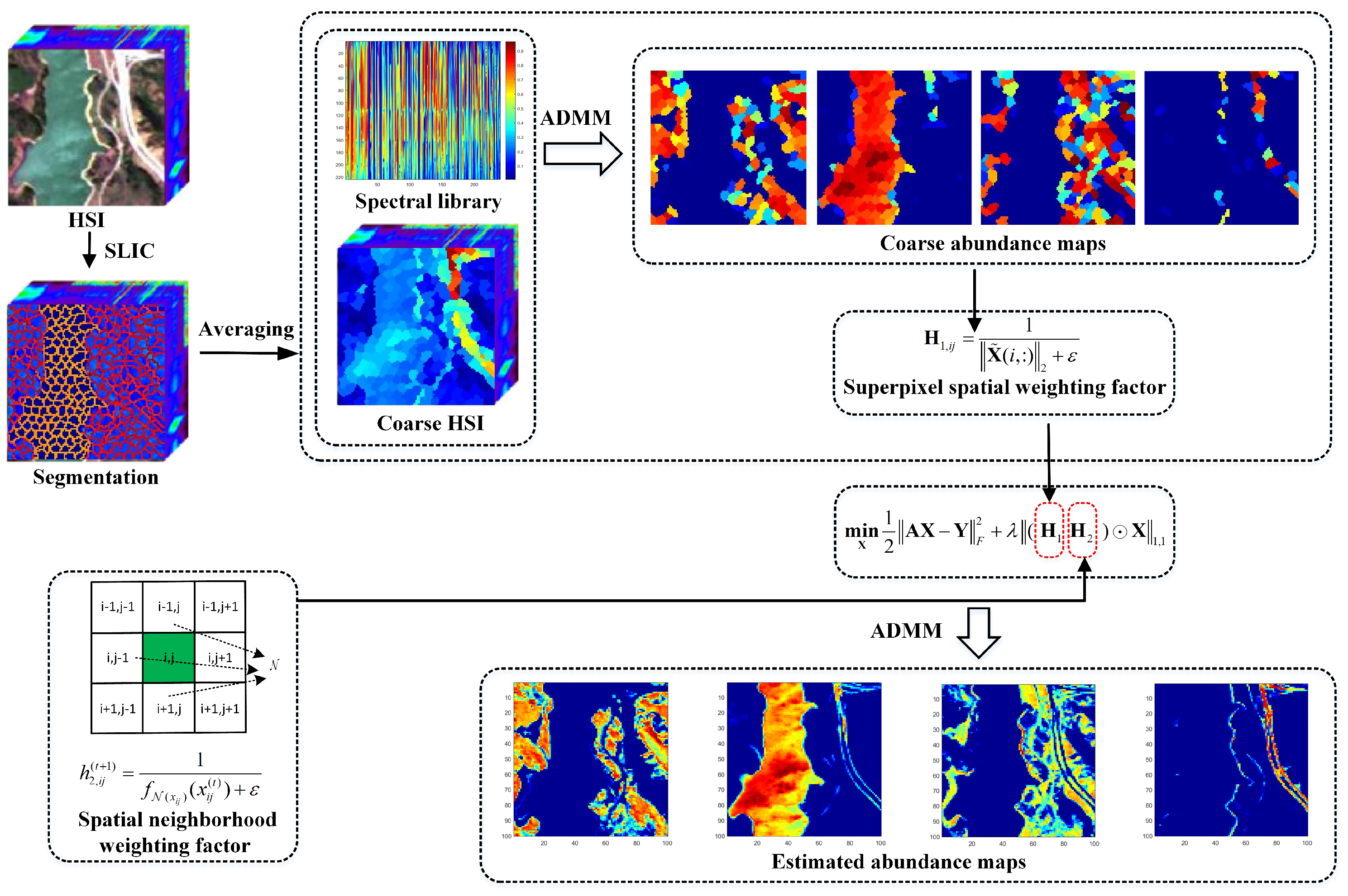
3.1. Proposed RDSWSU Method

Drawing on the achievements of the sparse unmixing technique utilizing reweighted 1 -norm, it can effectively impose a penalty on the abundance coefficients. This paper presents a novel approach called the robust dual spatial weighted sparse unmixing algorithm (RDSWSU) to address the challenges of noise reduction in unmixing and improve the spatial smoothness of abundance mapping. The flowchart of the proposed RDSWSU method is shown in Figure 1.
To enhance the robustness of the unmixing algorithm against noise, the superpixel spatial weight H 1 is constructed based on a coarse hyperspectral image, serving as a guidance for abundance estimation. It should be noted that the coarse hyperspectral image is reconstructed by a superpixel segmentation algorithm, which considered the similarity of pixels in terms of both spatial location and spectral characteristics. This reconstruction process resembles a mean filter and effectively suppresses noise in the image. Subsequently, a coarse-scale weight guide matrix is established predictively using the reconstructed hyperspectral image. H 1 is then calculated row by row from the coarse-scale weight guide matrix, making it insensitive to noise. Overall, the RDSWSU algorithm does not involve any denoising process. Instead, it mitigates the impact of noise on unmixing by performing superpixel segmentation on the original hyperspectral image and constructing superpixel spatial weights based on the segmented image. The optimization objective of the proposed RDSWSU algorithm can be defined as follows.
min X 1 2 | | A X Y | | F 2 + λ ( H 1 H 2 ) X 1 , 1 s . t . : X 0 .
where the operator ⊙ represents the elementwise multiplication of two variables. It should be noted that H 1 R m × m is the pre-calculated superpixel spatial weighting matrix, and H 2 R m × n is the spatial neighborhood weighting matrix.
As stated earlier, superpixel segmentation technology [43,50] refers to a method utilized for extracting spatial information from hyperspectral images. This technique allows for the analysis and characterization of the spatial structure within the image.
The superpixel spatial weighting matrix H 1 is designed to preserve the original spatial contextual information of hyperspectral images, particularly in scenarios with high levels of noise. Its purpose is to ensure that the spatial details in the image are accurately represented, even under challenging conditions with significant noise interference. To obtain the superpixel spatial weighting matrix H 1 , the initial hyperspectral image Y R L × n is segmented into g superpixel blocks using the SLIC algorithm [36,51]. Importantly, the SLIC algorithm is fast, simple to implement, and produces superpixels of good quality. It balances segmentation performance against computational complexity, serving as a useful and efficient image oversegmentation approach. This segmentation process divides the image into compact and homogeneous regions, each referred to as a superpixel block. By utilizing the SLIC algorithm, the hyperspectral image is effectively partitioned into g coherent and visually meaningful superpixels. Let Y t R L × n t ( t = 1 , , g , t = 1 g n t = n ) represent the t-th superpixel block, which consists of n t pixels. Within this block, we can refer to any pixel (column) as y k R L × 1 ( k = 1 , , n t ) . This notation allows us to refer to and manipulate individual pixels within specific superpixel blocks for further analysis or computations. Then, based on the segmentation result, the pixels within each superpixel block are averaged to obtain the coarse image Y ˜ R L × n . The statement is reformulated as follows.
y ˜ k = 1 n t k = 1 n t y k
In the given context, when referring to y ˜ k , it represents a column from the coarse image Y ˜ t that corresponds to a superpixel block in Y t . It is important to note that all elements within a single superpixel block possess identical values.
The SUnSAL method [17] is utilized to derive the coarse fractional abundance matrix X ˜ . The corresponding optimization model is expressed as follows.
min X ˜ 1 2 | | A X ˜ Y ˜ | | F 2 + λ | | X ˜ | | 1 , 1 , s . t . : X ˜ 0 .
where the low-resolution fractional abundance matrix X ˜ can keep the spatial information among the pixels. Finally, the superpixel-based weighting factor H 1 can be calculated as follows:
H 1 , i j = 1 | | X ˜ ( i , : ) | | 2 + ε , i = 1 , , m , j = 1 , , n
where ε > 0 represents a small constant. The ith row vector of the abundance matrix X ˜ is represented as X ˜ ( i , : ) , where ( i = 1 , , m ) . H 1 is influenced by the coarse abundance matrix X ˜ and can increase the sparsity of the row in the fractional abundance matrix.
Moreover, all the entries in each homogeneous region are averaged by the coarse hyperspectral image, so the impact of noise can be mitigated effectively. Therefore, the superpixel-based weighting matrix H 1 is not sensitive to noise.
To enhance the smoothness of abundance maps, the spatial weighting matrix H 2 takes into account the correlation between neighboring regions, following a similar approach as described in [52]. Let h 2 , i j t + 1 represent the entry in the t + 1 iteration of the weight matrix H 2 at the ith row and jth column. The spatial weighting factor H 2 can be iteratively updated as follows:
h 2 , i j ( t + 1 ) = 1 f N ( x i j ) ( x i j ( t ) ) + ε
where N ( x i j ) is the adjacent set for elements x i j , f ( · ) is a function that calculates the fractional abundance of pixels using a neighborhood system, with the goal of utilizing spatial correlations in images.
In this work, a new value of a pixel can be calculated by using the values of its 8-neighboring pixels and their importance (i.e., Euclidean distance). The function f ( · ) can be defined as follows:
f N ( x i j ) ( x i j ) = x a N 8 ( x i j ) Λ a x a x a N 8 ( x i j ) Λ a
where N 8 ( x i j ) represents adjacent elements ( x a ) of the central pixel x i j . Λ = 1 i m ( x a , x i j ) represents the neighboring importance. Where the function i m ( · ) represents the importance of the elements x a and x i j . Considering the European distance, Λ a is written as follows: Λ a = 1 / ( ( u m ) 2 + ( v n ) 2 ) 1 / 2 , where ( u , v ) and ( m , n ) represent the spatial coordinates of x a and x i j , respectively.

3.2. Optimization Model with the ADMM

In order to address the optimization difficulties of model (5), we adopt the ADMM technique as a solution method. The central concept of the ADMM method involves introducing a set of additional variables and subsequently transforming it into a sequence of more manageable sub-problems derived from the original problem. The optimization problem expressed as Equation (5) can be reformulated in the following manner.
min X , V 1 , V 2 , V 3 1 2 V 1 Y F 2 + λ ( H 1 H 2 ) V 2 1 , 1 + ι R + ( V 3 ) s . t . : V 1 = AX , V 2 = X , V 3 = X
the equation states that ι R + ( X ) = i = 1 n ι R + ( x i ) is an indicator function, and ι R + ( x i ) = 0 if x i belongs to the nonnegative orthant and ι R + ( x i ) = + otherwise.
Define V ( V 1 , V 2 , V 3 ) T , G = [ A , I , I ] T and B = diag ( I ) , where I is the identity matrix, and
g ( V ) 1 2 V 1 Y F 2 + λ ( H 1 H 2 ) V 2 1 , 1 + ι R + ( V 3 )
We can express Equation (10) in a condensed form as follows.
min X , V g ( V ) subject to GX + BV = 0 ,
We can denote the augmented Lagrangian function as given below.
L ( X , V , D ) g ( V ) + μ 2 GX + BV D F 2
where μ > 0 represents a positive constant, and D = ( D 1 , D 2 , D 3 ) T is the Lagrange multiplier related to the constraint GX + BV = 0 . Subsequently, we can minimize the augmented Lagrangian function L ( X , V , D ) to obtain the values for X and V . Simultaneously, we update D according to the following procedure.
X ( k + 1 ) = arg min X L ( X , V ( k ) , D ( k ) ) V ( k + 1 ) = arg min V L ( X ( k + 1 ) , V , D ( k ) ) D ( k + 1 ) = D ( k ) G X ( k + 1 ) B V ( k + 1 )
Afterwards, we can utilize the aforementioned framework to calculate the X and V -problems. First, the equivalent solution of the X subproblem is as follows.
min X μ 2 AX V 1 ( k ) D 1 ( k ) F 2 + μ 2 X V 2 ( k ) D 2 ( k ) F 2 + μ 2 X V 3 ( k ) D 3 ( k ) F 2
The solution for X is denoted as
X ( k + 1 ) = ( A T A + 2 I ) 1 ( A T ξ 1 + ξ 2 + ξ 3 )
where A T denotes the transpose of matrix A , and ξ 1 = V 1 ( k ) + D 1 ( k ) , ξ 2 = V 2 ( k ) + D 2 ( k ) , ξ 3 = V 3 ( k ) + D 3 ( k ) .
The subproblem of V decouples into three subparts about V 1 , V 2 , and V 3 . V 1 is calculated as follows:
min V 1 1 2 V 1 Y F 2 + μ 2 A X ( k + 1 ) V 1 D 1 ( k ) F 2
It clearly follows that
V 1 ( k + 1 ) = 1 1 + μ Y + μ ( AX ( k + 1 ) D 1 ( k ) )
V 2 is obtained by solving the problem using the following method.
min V 2 λ ( H 1 H 2 ) V 2 1 , 1 + μ 2 X ( k + 1 ) V 2 D 2 ( k ) F 2
The solution is
V 2 ( k + 1 ) = soft ( X ( k + 1 ) D 2 ( k ) , λ μ H 1 H 2 )
the function soft ( · , τ ) represents a soft-threshold function, which is defined as soft ( y , τ ) = sign ( y ) max { | y | τ , 0 } .
For the V 3 , it can be obtained by solving as
min V 3 ι R + ( V 3 ) + μ 2 X ( k + 1 ) V 3 D 3 ( k ) F 2
The solution is
V 3 ( k + 1 ) = max ( X ( k + 1 ) D 3 ( k ) , 0 )
Lastly, the Lagrange multipliers are updated in the following manner.
D 1 ( k + 1 ) = D 1 ( k ) A X ( k + 1 ) + V 1 ( k + 1 ) D 2 ( k + 1 ) = D 2 ( k ) X ( k + 1 ) + V 2 ( k + 1 ) D 3 ( k + 1 ) = D 3 ( k ) X ( k + 1 ) + V 3 ( k + 1 )
To summarize, Algorithm 1 outlines the use of the ADMM method to solve the optimization problem in the RDSWSU model. The RDSWSU algorithm, suggested in the study, is composed of an inner loop and an outer loop. In the inner loop, the Lagrange multipliers in the ADMM method are updated. On the other hand, the weight coefficients are updated in the outer loop. The maximum number of iterations in the inner loop is set to 5, while the number of iterations in the outer loop is set to 120. The iterative optimization of the model is similar to the well-known SUnSAL method in complexity due to the simplicity of the model.
Proving formal convergence for Algorithm 1 is difficult, however empirically the residual of the original problem is seen to decrease with more iterations. As illustrated in Figure 2, the residual GX ( t ) + BV ( t ) F 1 × 10 5 as a function of outer loop counts reaches a stable near-zero level after only 40 iterations. The dual loop structure exhibits good empirical convergence and speed overall. The full algorithm halts when hitting the maximum iterations or once the residual satisfies a tolerance threshold.
Algorithm 1: The pseudocode representation for RDSWSU
1: Input: Y, A, and parameters of the SLIC algorithm
2: Perform:
3: Use the SLIC algorithm to segment image Y.
4: Compute Equation (6) to reconstruct the Y ˜
5: X ˜ obtained by solving the optimization problem (7)
6: H 1 , i j 1 | | X ˜ ( i , : ) | | 2 + ε
7: Initialization:
8: set k , t = 0 , choose λ , μ , ε > 0 , X ( 0 ) , V 1 ( 0 ) , V 2 ( 0 ) , V 3 ( 0 ) , D 1 ( 0 ) , D 2 ( 0 ) , D 3 ( 0 )
9: Repeat:
10: H 2 ( t + 1 ) h 2 , 11 ( t ) h 2 , 1 n ( t ) h 2 , i j ( t ) h 2 , m 1 ( t ) h 2 , m n ( t ) ,
11: where h 2 , i j ( t + 1 ) = 1 f N ( x i j ) ( x i j ( t ) d 2 , i j ( t ) ) + ε , x i j and d 2 , i j are respectively the elements in the ith row and jth column of X and D 2 .
12: Repeat:
13: X ( k + 1 ) ( A T A + 2 I ) 1 A T ( V 1 ( k ) + D 1 ( k ) ) + V 2 ( k ) + D 2 ( k ) + V 3 ( k ) + D 3 ( k )
14: V 1 ( k + 1 ) 1 1 + μ Y + μ ( A X ( k + 1 ) D 1 ( k ) )
15: V 2 ( k + 1 ) soft ( X ( k + 1 ) D 2 ( k ) , λ μ H 1 H 2 ( t ) )
16: V 3 ( k + 1 ) max ( X ( k + 1 ) D 3 ( k ) , 0 )
17: Revise the Lagrange multipliers:
18: D 1 ( k + 1 ) D 1 ( k ) A X ( k + 1 ) + V 1 ( k + 1 )
19: D 2 ( k + 1 ) D 2 ( k ) X ( k + 1 ) + V 2 ( k + 1 )
20: D 3 ( k + 1 ) D 3 ( k ) X ( k + 1 ) + V 3 ( k + 1 )
21: Refresh the iteration:  k k + 1
22: X ( t + 1 ) X ( k )
23: D 2 ( t + 1 ) D 2 ( k )
24: Refresh the iteration:  t t + 1
25: until certain stopping criteria are satisfied.

4. Experiments with Synthetic Data

In these experiments, we will showcase the performance of the proposed RDSWSU method by conducting two simulated hyperspectral datasets. In our experiments, we will conduct a comparison between the proposed RDSWSU method and five other advanced sparse unmixing methods: SUnSAL [17], SUnSAL-TV [29], DRSU [27], DRSU-TV [31] and S 2 WSU [52]. It is worth mentioning that the last three algorithms utilize weighted sparse regression techniques.
Furthermore, two commonly utilized quality metrics are employed to assess the efficacy of sparse unmixing. The signal reconstruction error ratio (SRE), measured in decibels (dB), is a commonly used metric in quantitative analysis. It serves as an indicator to evaluate the accuracy of unmixing and gauge the performance of various unmixing algorithms. The calculation formula of SRE (dB) is:
SRE ( dB ) = 10 · log 10 E ( | | x | | 2 2 ) E ( | | x x ^ | | 2 2 )
where x ^ denotes the estimated fractional abundance, x denotes the true fractional abundance, and E ( · ) indicates the expected function. The greater the value of SRE (dB), the higher the quality of unmixing achieved by this method.
In addition, we also adopt another measure, that is, the probability of success p s . It represents an estimation of the likelihood that the relative error in power is below a certain threshold. The p s can be obtained by formally calculating as follows: p s P ( x ^ x 2 / x 2 t h r e s h o l d ) . In previous studies [17], it has been shown that the abundance estimation is deemed successful when x ^ x 2 / x 2 3.16 (5 dB). The unmixing performance improves as the p s value increases.

4.1. Simulated Data Sets

In this paper, we utilized two spectral libraries in the synthetic data analysis, both of which were extracted from the mineral dictionary of the US Geological Survey (USGS) spectral library (Available online at http://speclab.cr.usgs.gov/spectral.lib06 (accessed on 21 June 2023)). The spectral library A 1 R 224 × 240 comprises m = 240 spectral signatures with reflectance values across L = 224 spectral bands, evenly distributed within the wavelength range of 0.4–2.5 μ m. Similar to A 1 , the spectral library A 2 R 221 × 222 consists of m = 222 spectral signatures with L = 221 spectral bands. According to LMM, two distinct simulated datasets were generated from spectral libraries A 1 and A 2 . The fractional abundances were enforced with ANC and ASC constraints. Subsequently, a detailed description of the two simulated datasets will be provided.
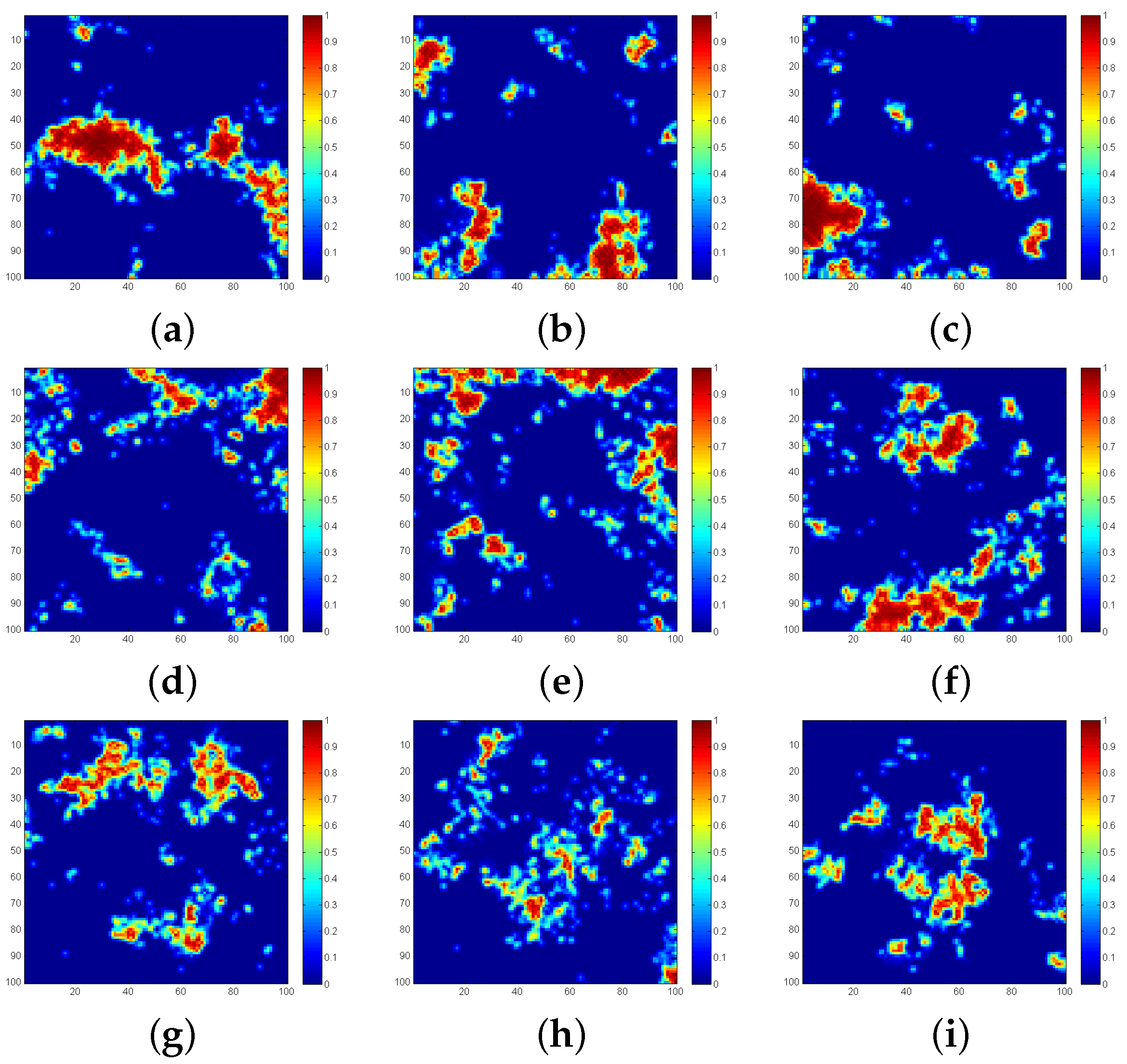
  • Simulated Data Cube 1 (DC1): DC1 comprises 100 × 100 pixels, with each pixel containing 224 spectral bands. DC1 was generated by randomly selecting nine spectral signatures from spectral library A 1 . Figure 3 illustrates the actual abundance maps associated with the nine endmembers. The simulated hyperspectral data generation process involved the introduction of independent and identically distributed (i.i.d.) Gaussian noise at five different SNR levels: 10 dB, 20 dB, 30 dB, 40 dB, and 50 dB.
  • Simulated Data Cube 2 (DC2): DC2 has 100 × 100 pixels, with each pixel containing 221 spectral bands. Simulated data DC2 was generated by randomly selecting nine spectral signatures from spectral library A 2 , as detailed in [53,54]. Figure 4 displays the genuine abundance maps corresponding to the nine endmembers. In the experiments, similar to DC1, the simulated data for DC2 was also subjected to independent and i.i.d. Gaussian noise at five different SNR levels: 10 dB, 20 dB, 30 dB, 40 dB, and 50 dB.

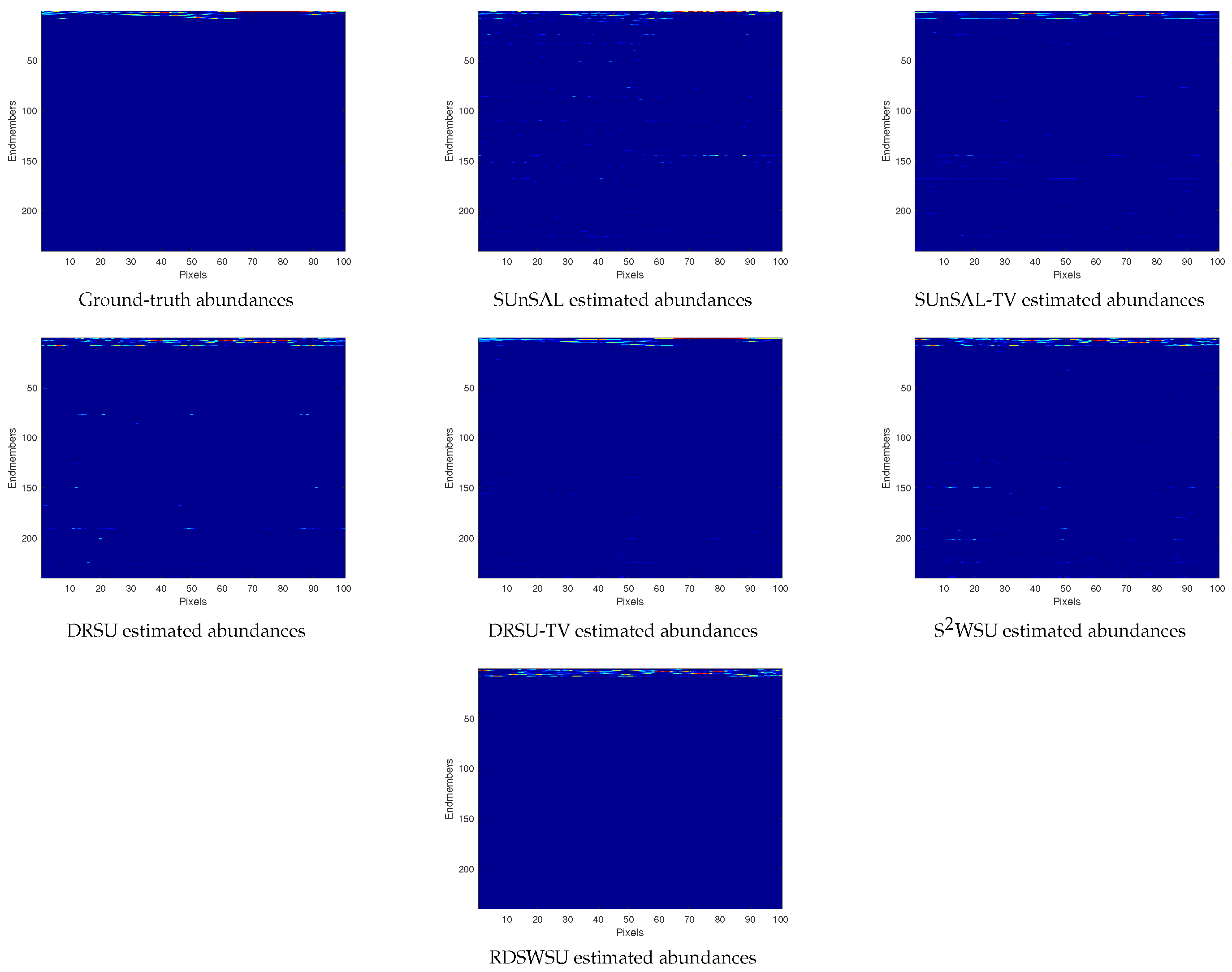
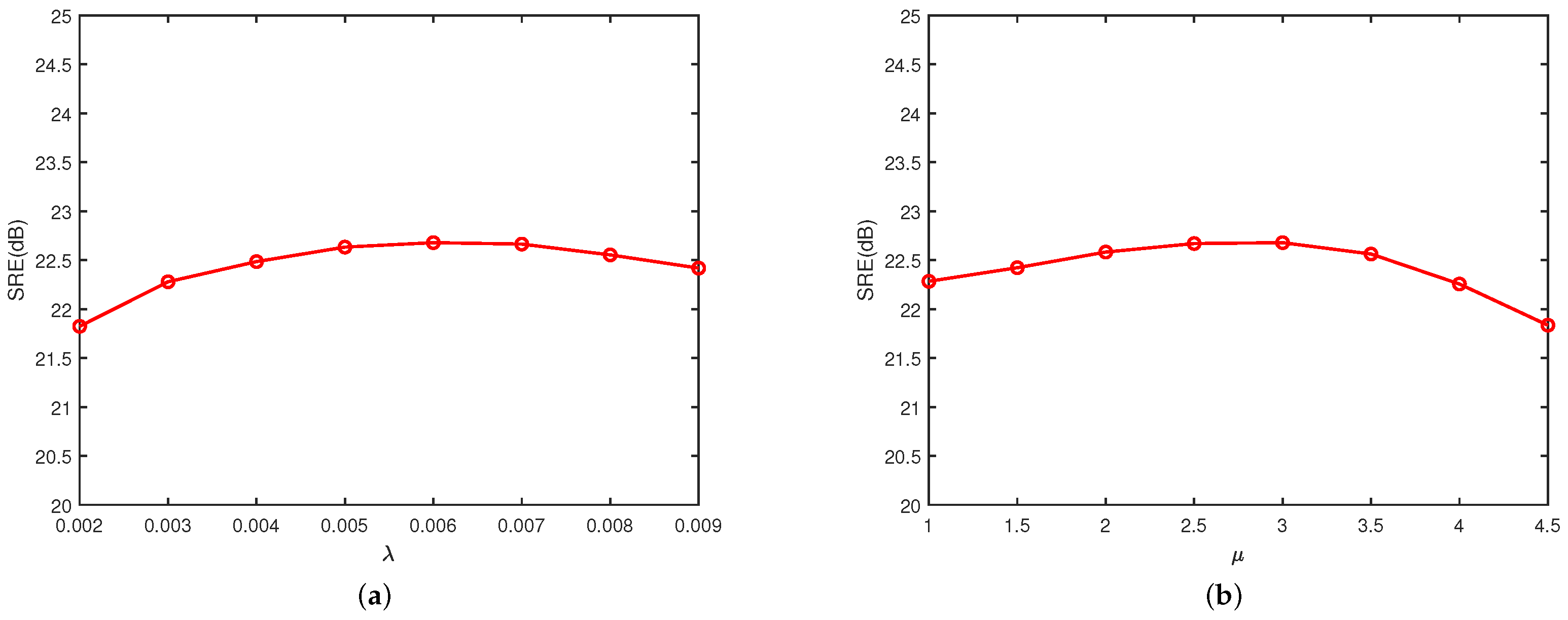
4.2. Results and Discussion

In this section, we use two simulated datasets to test the proposed unmixing performance based on a dual spatial weighting strategy. For the parameter settings in the experiments, each method was tested with different combinations of parameter settings to ensure the optimal results. Table 1 and Table 2 exhibit the SRE (dB) and p s values obtained by each tested unmixing method on the two simulated datasets at different SNR levels. The tables show the optimal values obtained within the specified parameter range.
Table 1 and Table 2 demonstrate a trend where the performance of the listed algorithms for unmixing worsens as the noise level increases. Compared with other methods, the RDSWSU method achieves the highest SRE (dB) values across all noise levels. It is noteworthy that the proposed algorithm exhibits a significant advantage in low signal-to-noise ratio situations, and can achieve more accurate separation performance. For example, in DC1 and DC2, when the SNR is 10 dB (i.e., in high noise conditions), our method has increased the SRE (dB) by more than 2 dB compared to other methods, indicating that the RDSWSU method has stronger noise resistance. Furthermore, compared with several other algorithms, the algorithm presented in this paper also achieves superior results in terms of p s value, especially in low SNR conditions, which validates the high robustness of the dual-spatial weighting strategy. In summary, based on the dual-spatial weighting strategy, it has provided a good prospect for improving the unmixing accuracy in two different scenes.
To facilitate a direct comparison between different unmixing algorithms, we select DC1 and DC2 as examples at an SNR of 20 dB. This selection aims to demonstrate the improved sparsity of the solution achieved by the proposed RDSWSU algorithm. Figure 5 and Figure 6 demonstrate the corresponding fractional abundances estimated by each unmixing algorithm and the ground-truth abundances. It should be noted that each line represents a nonzero vector of the abundance matrix (with 100 randomly selected pixels shown here for display). It is evident that both the SUnSAL and SUnSAL-TV algorithms produce inaccurate estimations of the number of recovered endmembers. In contrast, the RDSWSU algorithm exhibits a remarkable ability to accurately estimate the number of endmembers, surpassing the performance of the DRSU, DRSU-TV, and S 2 WSU algorithms in this regard. Therefore, compared with SUnSAL-TV, DRSU, DRSU-TV, and S 2 WSU, the proposed RDSWSU algorithm can accurately identify the optimal subset of endmembers from the spectral library. Compared with other unmixing methods, the RDSWSU algorithm improved the ability to identify endmembers from a spectral library while also enhancing the sparsity of the abundance matrix.
Figure 7 and Figure 8 present the abundance maps of the first endmember achieved using various unmixing algorithms in DC1 and DC2 when the SNR is set to 20 dB. For a more intuitive comparison, the difference maps, which are generated by subtracting the estimated abundances from the ground truth abundances, are also shown in the figures. From Figure 7 and Figure 8, it can be observed that the abundance maps derived from SUnSAL and SUnSAL-TV lack accuracy. The abundance maps generated by the SUnSAL algorithm exhibit noticeable noise, indicating a relatively high level of noise present in the results. The SUnSAL-TV algorithm, on the one hand, enhances the quality of abundance estimation to some extent by incorporating spatial information. On the other hand, the abundance maps produced by the SUnSAL-TV algorithm appear over-smoothness phenomenon and blurred in their visual representation. The unmixing outcomes achieved by RDSWSU exhibit a remarkable resemblance to the true abundance maps, distinguishing it from other algorithms. Additionally, its abundance maps demonstrate a greater amount of spatial detail information across various homogeneous regions. In Figure 7 and Figure 8, it is evident that the abundance map obtained by the RDSWSU algorithm is smoother at the boundary compared to the results of the SUnSAL, DRSU, and S 2 WSU algorithms. However, it does not exhibit over-smoothing like the SUnSAL-TV and DRSU-TV algorithms. The RDSWSU algorithm integrates the dual spatial weighting factor with the estimated abundance through element-wise multiplication, and minimizes the 1 norm of their product. Thereinto, the superpixel spatial weighting factor is established at the scale of superpixels, where each superpixel corresponds to a homogeneous region in the image. During the unmixing process, the pixels within the same superpixel block are assigned identical weights, while the weights for pixels in different superpixel blocks differ. In a sense, the superpixel spatial weighting factor helps to preserve the spatial heterogeneity of the image. Furthermore, even within a superpixel, the final weight of each pixel can vary because there is another spatial neighborhood weighting factor that affects the final weight. The spatial neighborhood weighting factor is determined by the abundance vectors of its neighboring pixels within an 8-neighborhood. Each pixel is assigned a unique weight and dynamically changes with iterations. Unlike the TV regularization that directly constrains the differences in the abundance vectors of each pixel in the horizontal and vertical directions, the spatial neighborhood weighting factor induces the pixel with lower neighboring abundance to have an even lower abundance, rather than forcing its abundance to be equal to that of the neighboring pixels. As a result, the dual spatial weighting factor effectively utilizes the spatial correlation between pixels while also maintaining the heterogeneity of different homogeneous regions and promoting sparsity of abundance, thus avoiding excessive smoothing. It is proved that the weight factors based on superpixels and spatial neighborhood can significantly improve the effect of sparse unmixing.
Table 3 shows the computational time taken by different algorithms to process DC1 at SNR = 20 dB. All algorithms were coded using MATLAB (R2018b) and tested in a standardized computing environment. The testing was conducted on a desktop computer equipped with an Intel Core i7 dual-core processor running at 3.6 GHz and 16 GB of RAM.
It is noteworthy that the RDSWSU method did not include the time for superpixel segmentation and spatial weighting computation in its computational time, as both of these steps were preprocessed and the generated weight values were introduced as constants. Consequently, there is no necessity to recompute or make adjustments to the superpixel segmentation and spatial weighting while performing the unmixing procedure. By referring to Table 3, it can be noted that the SUnSAL algorithm exhibits the shortest processing time. On the other hand, the remaining algorithms are comparatively slower as they are derived from the SUnSAL algorithm. The SUnSAL-TV and DRSU-TV methods, which employ TV regularization, exhibit longer processing times due to the high computational cost associated with solving the TV spatial regularization term. This results in a longer duration compared to other algorithms. The processing times of the three algorithms without TV regularization are nearly identical, indicating that the proposed RDSWSU algorithm achieves superior unmixing performance in comparison to other algorithms without introducing additional computational complexity.
Furthermore, we examined the effects of varying the two ADMM parameters—regularization λ and Lagrangian multiplier μ - on unmixing performance. Using the DC1 dataset at 30 dB SNR as an example, Figure 9a shows our proposed RDSWSU algorithm can readily achieve suboptimal tuning by first fixing μ randomly, then selecting λ from a set. As Figure 9b demonstrates, μ selection is robust over a wide range, producing minimal variability in the results.

5. Experiments with Real Hyperspectral Data

We employ two real hyperspectral data sets in this section—the Cuprite data and Houston data—to assess the performance of the various algorithms.

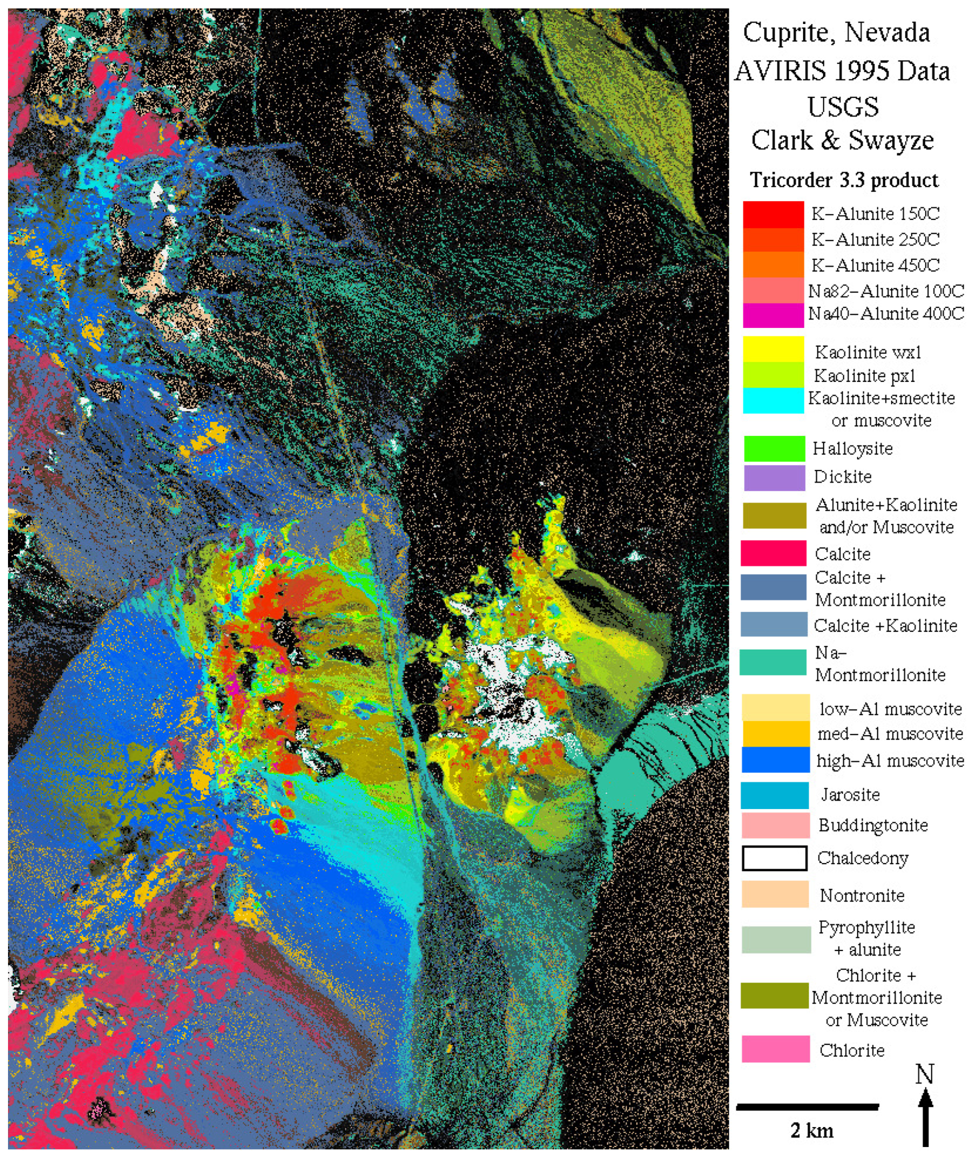
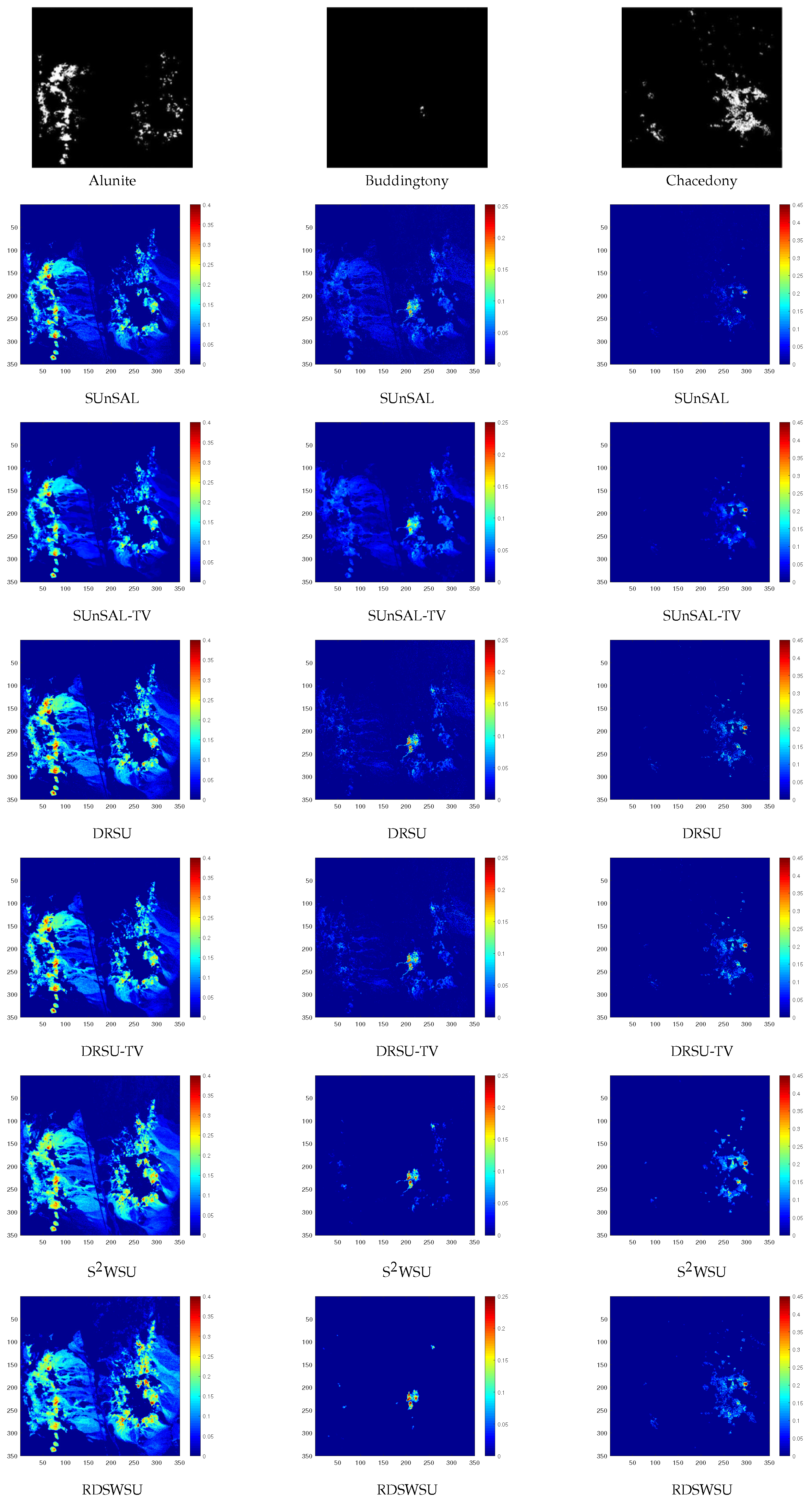
5.1. Experiment on Cuprite Data

The performance of the proposed method was evaluated using the well-known Cuprite dataset from the Airborne Visible/Infrared Imaging Spectrometer (AVIRIS). The Cuprite site holds significant recognition in the field of mineralogy. The scene has been extensively utilized as a benchmark for validating the effectiveness of unmixing algorithms due to several exposed minerals. The experimental part focuses on a subset of the scene that measures 350 × 350 pixels. This subset includes 224 spectral bands with wavelengths spanning from 0.4 to 2.5 μ m, and each band has a spectral resolution of 10 nm. Before conducting the analysis, certain bands were excluded due to their low water absorption and inadequate SNR. Specifically, bands 1–2, 105–115, 150–170, and 223–224 were removed from consideration. As a result, there were 188 spectral bands remaining for the analysis after the exclusion of the aforementioned bands. More specifically, the spectral library utilized in this experiment is equivalent to the spectral library A 1 that was employed in our simulation experiments. In addition, bands with a low SNR and those exhibiting low water absorption were also excluded from A 1 . Furthermore, Tricorder software was utilized to generate classification maps depicting the distribution of these minerals. Unfortunately, the classification map was producted in 1995, and the publicly accessible Cuprite data was collected in 1997, a direct comparison between the classification map and the AVIRIS Cuprite data is not feasible. Therefore, the classification accuracy is not provided. Nonetheless, the classification map proves to be a valuable tool for qualitatively assessing the fractional abundance maps generated by the unmixing algorithms. Figure 10 illustrates a mineral map drawn by the USGS utilizing Tricorder 3.3 software [55] to represent the spatial distribution of various minerals within the Cuprite mining area.
Figure 11 presents a visual comparison of the classification maps produced by the USGS Tricorder algorithm in real hyperspectral scenes, along with three distinct mineral abundance maps (Alunite, Buddingtonite, and Chalcedony) generated by the SUnSAL, SUnSAL-TV, DRSU, DRSU-TV, S 2 WSU, and RDSWSU algorithms. In this experiment, the regularization parameters were set as λ = 0.001 , λ = 0.0001 , λ = 0.002 , and λ = 0.003 for SUnSAL, DRSU, S 2 WSU, and RDSWSU, respectively. For SUnSAL-TV and DRSU-TV, the regularization parameters were set to λ = 0.001 , λ T V = 0.001 and λ = 0.002 , λ T V = 0.0001 , respectively. The reasonable unmixing results achieved by all methods in Figure 11 demonstrate the effectiveness of sparse unmixing algorithms in interpreting the considered real hyperspectral datasets. As shown in Figure 11, the abundance maps (such as Buddingtonite) produced by SUnSAL and SUnSAL-TV algorithms displayed many noisy points. The results obtained using the SUnSAL-TV algorithm display an over-smoothness phenomenon, particularly noticeable in the estimation of Alunite and Buddingtonite. Additionally, the abundance map generated by DRSU algorithm has a mediocre performance in terms of spatial consistency (e.g., Chalcedony). We can observe that compared to the DRSU-TV and S 2 WSU algorithms, the abundance map generated by RDSWSU algorithm (such as Buddingtonite) is more similar to the reference image and shows smaller noise, demonstrating good spatial detail information. Considering qualitative criteria, it can be inferred that the proposed RDSWSU method outperforms other methods in terms of interpretability for the given real hyperspectral scene. To quantitatively assess the unmixing results in the real hyperspectral data experiment, we introduce a new evaluation metric, known as sparsity. This metric quantifies the ratio of elements in the estimated abundance that exceed 0.005 to the total number of elements. A lower sparsity value indicates a more sparse unmixing outcome, aligning with the expectations of sparse regression-based unmixing algorithms. The sparsity achieved by SUnSAL, SUnSAL-TV, DRSU, DRSU-TV, S 2 WSU and RDSWSU is 0.0682, 0.0743, 0.0428, 0.0422, 0.0421, and 0.0408 respectively. From these minor differences, we can infer that the proposed method represents the data with fewer components, improving sparsity. This qualitative analysis indicates the potential of the newly proposed RDSWSU algorithm to boost unmixing capabilities in real-world applications.

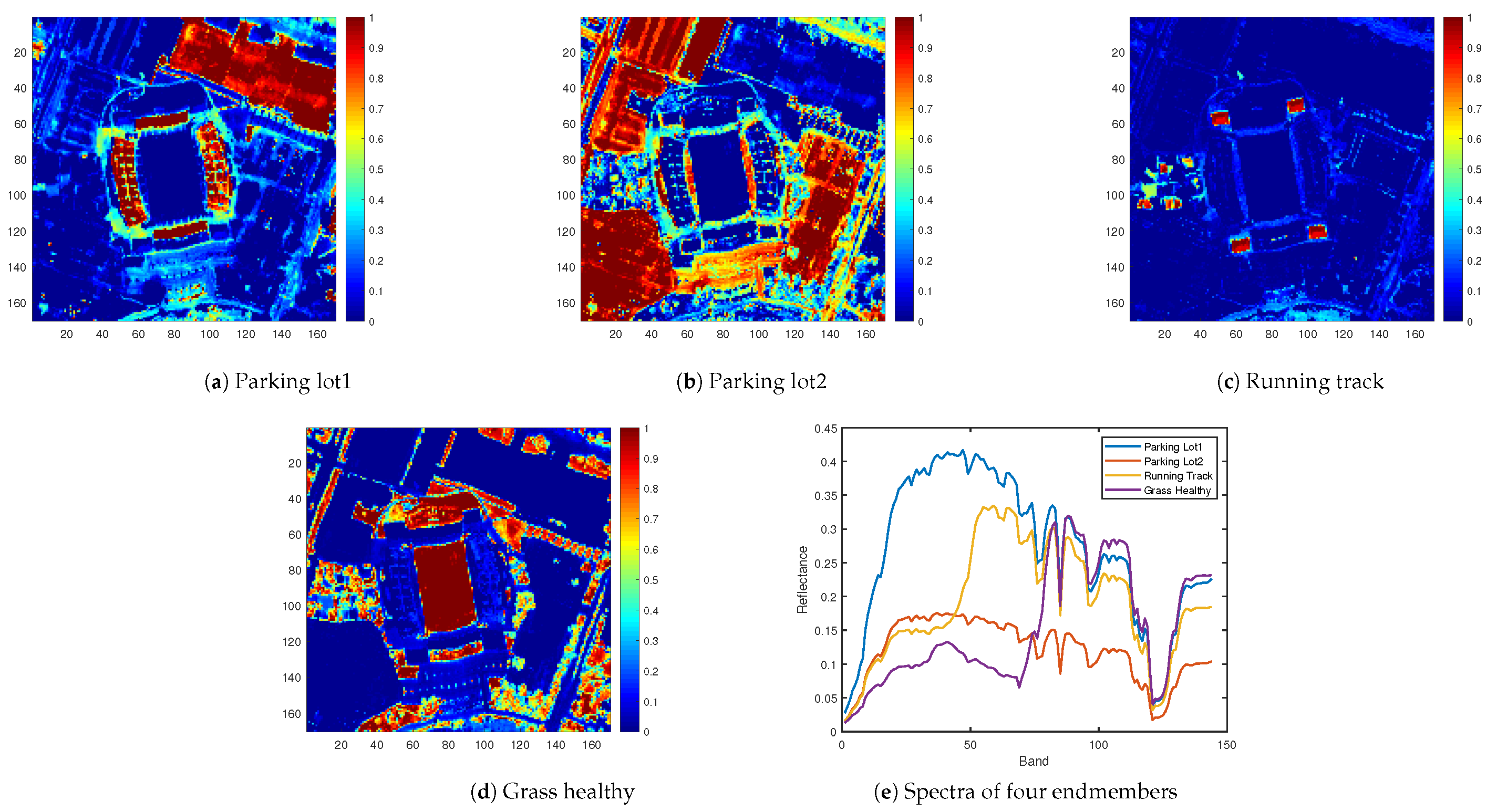
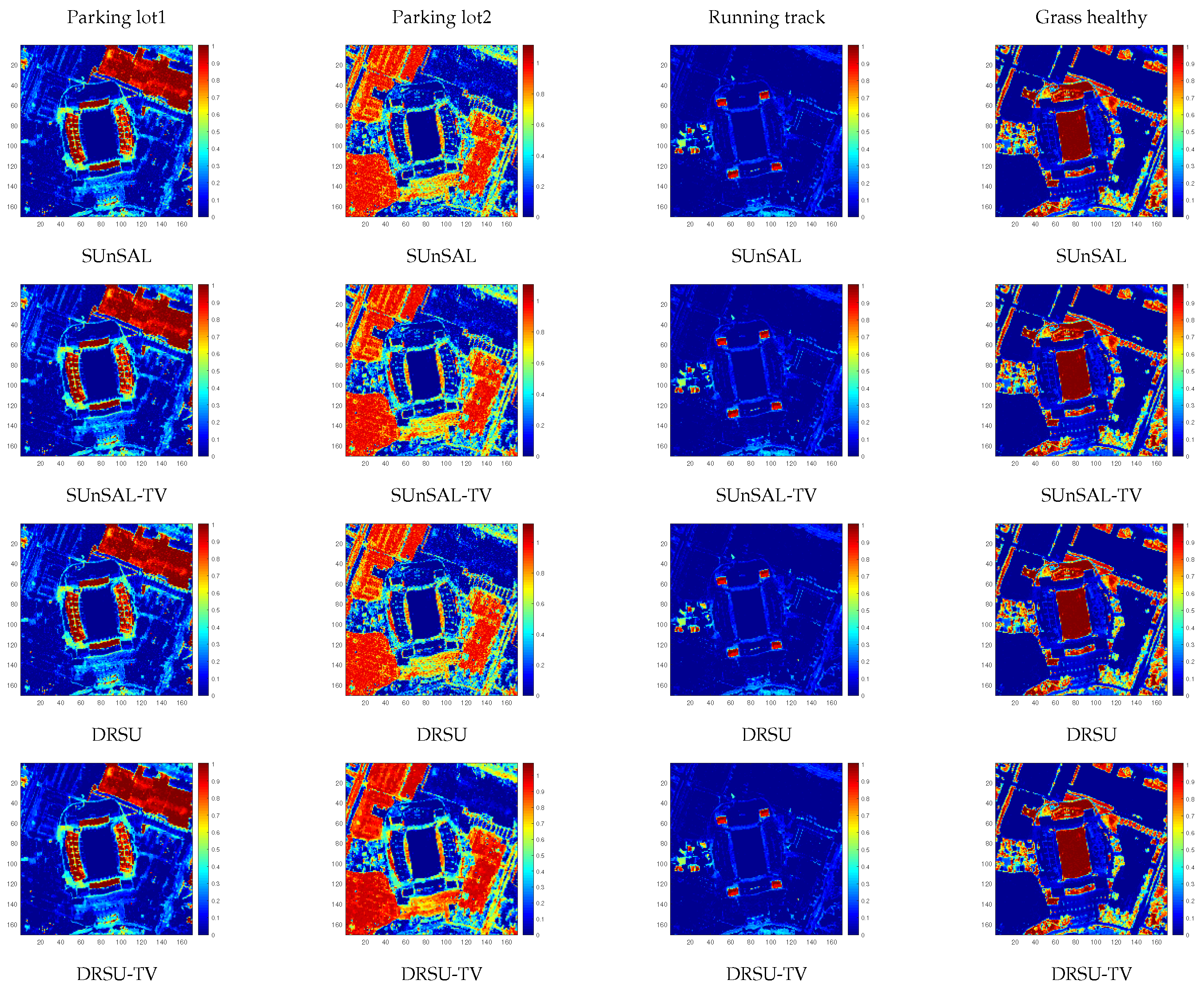
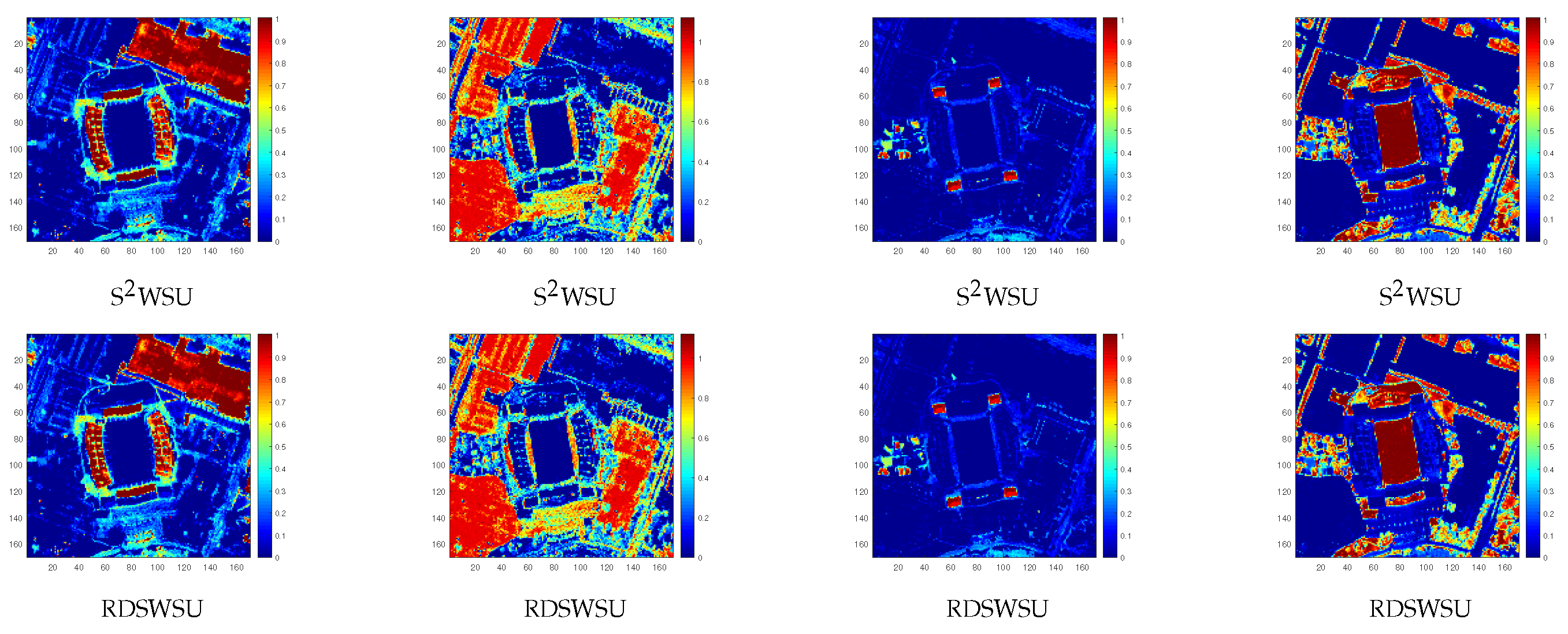
5.2. Experiment on Houston Data

In addition, we have introduced another commonly used benchmark dataset, the Houston dataset [56], for real hyperspectral data experiments to further demonstrate the superiority of the proposed RDSWSU algorithm. The Houston dataset was acquired by the ITRES CASI-1500 sensor over the University of Houston campus in June 2012 (Available online at http://hyperspectral.ee.uh.edu (accessed on 21 June 2023)). It comprises 170 × 170 pixels, with 144 spectral bands spanning 364 nm to 1046 nm. Four endmembers are present in the data: Running track, Parking lot1, Parking lot2 and Grass healthy. Figure 12 shows the Houston data along with the real abundance maps and spectral signatures of the four endmembers. Notably, the endmember spectral library A 3 R 144 × 4 used here only contains the actual spectral signatures of the four endmembers.
Figure 13 presents the abundance maps estimated by the six unmixing methods for the four endmembers. The obtained SRE (dB) values are 20.5499, 21.5405, 20.5757, 21.5473, 21.5537, and 21.5805 for SUnSAL, SUnSAL-TV, DRSU, DRSU-TV, S 2 WSU and RDSWSU, respectively. The quantitative results demonstrate our proposed method achieves comparable or slightly better performance versus other approaches. Notably, the differences are marginal, largely owing to the endmember spectral library containing only the four actual spectral signatures, which limits the full potential of weighted sparse unmixing algorithms. Still, the stable results from our method signify its merits.

6. Conclusions

This paper introduces a novel algorithm called robust dual spatial weighted sparse unmixing (RDSWSU) to enhance the outcomes of sparse unmixing. The RDSWSU algorithm presented in this study leverages superpixel-based spatial weighting and spatial neighborhood weighting factors for effectively utilizing the spatial information embedded in hyperspectral images. This can achieve accurate and stable unmixing results in high-noise environments. Additionally, this method utilizes an inner and outer loop strategy aimed at accelerating the convergence speed of the iterative optimization process of the model. The experimental results obtained from simulated and real hyperspectral datasets have showcased the remarkable capabilities of the proposed RDSWSU method. It exhibits substantial potential in enhancing unmixing performance, particularly in high-noise scenarios. While the experimental results obtained in this study are highly promising, it is important to acknowledge the need for conducting experiments on additional datasets in order to comprehensively assess the effectiveness of the proposed algorithm. In future endeavors, novel techniques such as low-rank prior [57] and deep learning [58] will be employed to effectively leverage the intrinsic feature information in images. This approach aims to enhance data interpretability and extract more valuable insights from the data.

Author Contributions

Conceptualization, C.D. and S.Z.; methodology, Y.C.; software, S.Z. and Y.C.; validation, M.H. and P.L.; writing—original draft preparation, Y.C.; writing—review and editing, S.Z.; supervision, F.L. and D.S.; funding acquisition and project administration, S.W. All authors have read and agreed to the published version of the manuscript.

Funding

This work was supported in part by the Training Program for Academic and Technical Leaders of Jiangxi Province under Grant 20225BCJ23019, in part by the Jiangxi Provincial Natural Science Foundation under Grant 20224ACB202002 and Grant 20224BAB202007, in part by the Chinese Ministry of Education Chunhui Plan Collaborative Research Project 202201108, in part by the Jiangxi Provincial Key Research and Development Program under Grant 20202BBGL73081, in part by the Guangdong Provincial Department of Housing and Urban-Rural Development Science and Technology Plan Project under Grant 2021-K1-140626, in part by the Science and Technology Project of Guangzhou Municipal Construction Group Co., Ltd. under Grant [2021]-KJ059.

Institutional Review Board Statement

Not applicable.

Informed Consent Statement

Not applicable.

Data Availability Statement

Not applicable.

Acknowledgments

The authors would like to gratefully thank the Editor, Associate Editor and the Anonymous Reviewers for their outstanding comments and suggestions, which greatly helped us to improve the technical quality and presentation of this manuscript.

Conflicts of Interest

The authors declare no conflict of interest.

References

  1. Bioucas-Dias, J.M.; Plaza, A.; Camps-Valls, G.; Scheunders, P.; Nasrabadi, N.; Chanussot, J. Hyperspectral Remote Sensing Data Analysis and Future Challenges. IEEE Geosci. Remote Sens. Mag. 2013, 1, 6–36. [Google Scholar] [CrossRef]
  2. He, L.; Li, J.; Liu, C.; Li, S. Recent Advances on Spectral-Spatial Hyperspectral Image Classification: An Overview and New Guidelines. IEEE Trans. Geosci. Remote Sens. 2018, 56, 1579–1597. [Google Scholar] [CrossRef]
  3. Qi, J.; Gong, Z.; Yao, A.; Liu, X.; Li, Y.; Zhang, Y.; Zhong, P. Bathymetric-Based Band Selection Method for Hyperspectral Underwater Target Detection. Remote Sens. 2021, 13, 3798. [Google Scholar] [CrossRef]
  4. Lu, B.; Dao, P.D.; Liu, J.; He, Y.; Shang, J. Recent Advances of Hyperspectral Imaging Technology and Applications in Agriculture. Remote Sens. 2020, 12, 2659. [Google Scholar] [CrossRef]
  5. Sankey, T.; Donager, J.; McVay, J.; Sankey, J.B. UAV lidar and hyperspectral fusion for forest monitoring in the southwestern USA. Remote Sens. Environ. 2017, 195, 30–43. [Google Scholar] [CrossRef]
  6. Tan, Y.; Lu, L.; Bruzzone, L.; Guan, R.; Chang, Z.; Yang, C. Hyperspectral Band Selection for Lithologic Discrimination and Geological Mapping. IEEE J. Sel. Topics Appl. Earth Observ. Remote Sens. 2020, 13, 471–486. [Google Scholar] [CrossRef]
  7. Tu, B.; Wang, Z.; Ouyang, H.; Yang, X.; Li, J.; Plaza, A. Hyperspectral Anomaly Detection Using the Spectral-Spatial Graph. IEEE Trans. Geosci. Remote Sens. 2022, 60, 1–14. [Google Scholar] [CrossRef]
  8. Bioucas-Dias, J.; Plaza, A.; Dobigeon, N.; Parente, M.; Du, Q.; Gader, P.; Chanussot, J. Hyperspectral Unmixing Overview: Geometrical, Statistical, and Sparse Regression-Based Approaches. IEEE J. Sel. Topics Appl. Earth Observ. Remote Sens. 2012, 5, 354–379. [Google Scholar] [CrossRef]
  9. Keshava, N.; Mustard, J. Spectral unmixing. IEEE Signal Process. Mag. 2002, 19, 44–57. [Google Scholar] [CrossRef]
  10. Hong, D.; Gao, L.; Yao, J.; Yokoya, N.; Chanussot, J.; Heiden, U.; Zhang, B. Endmember-Guided Unmixing Network (EGU-Net): A General Deep Learning Framework for Self-Supervised Hyperspectral Unmixing. IEEE Trans. Neural Netw. Learn. Syst. 2022, 33, 6518–6531. [Google Scholar] [CrossRef]
  11. Nascimento, J.; Bioucas-Dias, J. Vertex component analysis: A fast algorithm to unmix hyperspectral data. IEEE Trans. Geosci. Remote Sens. 2005, 43, 898–910. [Google Scholar] [CrossRef]
  12. Li, J.; Agathos, A.; Zaharie, D.; Bioucas-Dias, J.; Plaza, A.; Li, X. Minimum Volume Simplex Analysis: A Fast Algorithm for Linear Hyperspectral Unmixing. IEEE Trans. Geosci. Remote Sens. 2015, 53, 5067–5082. [Google Scholar]
  13. Zhang, S.; Agathos, A.; Li, J. Robust Minimum Volume Simplex Analysis for Hyperspectral Unmixing. IEEE Trans. Geosci. Remote Sens. 2017, 55, 6431–6439. [Google Scholar] [CrossRef]
  14. Li, Z.; Altmann, Y.; Chen, J.; Mclaughlin, S.; Rahardja, S. Sparse Linear Spectral Unmixing of Hyperspectral Images Using Expectation-Propagation. IEEE Trans. Geosci. Remote Sens. 2022, 60, 1–13. [Google Scholar] [CrossRef]
  15. Nascimento, J.M.; Bioucas-Dias, J. Does independent component analysis play a role in unmixing hyperspectral data. IEEE Trans. Geosci. Remote Sens. 2005, 43, 175–187. [Google Scholar] [CrossRef]
  16. Li, F.; Zhang, S.; Liang, B.; Deng, C.; Xu, C.; Wang, S. Hyperspectral Sparse Unmixing With Spectral-Spatial Low-Rank Constraint. IEEE J. Sel. Top. Appl. Earth Observ. Remote Sens. 2021, 14, 6119–6130. [Google Scholar] [CrossRef]
  17. Iordache, M.D.; Bioucas-Dias, J.; Plaza, A. Sparse Unmixing of Hyperspectral Data. IEEE Trans. Geosci. Remote Sens. 2011, 49, 2014–2039. [Google Scholar] [CrossRef]
  18. Zhang, G.; Mei, S.; Xie, B.; Ma, M.; Zhang, Y.; Feng, Y.; Du, Q. Spectral Variability Augmented Sparse Unmixing of Hyperspectral Images. IEEE Trans. Geosci. Remote Sens. 2022, 60, 1–13. [Google Scholar] [CrossRef]
  19. Zhang, X.; Yuan, Y.; Li, X. Reweighted Low-Rank and Joint-Sparse Unmixing With Library Pruning. IEEE Trans. Geosci. Remote Sens. 2022, 60, 1–16. [Google Scholar] [CrossRef]
  20. Tang, W.; Shi, Z.; Wu, Y.; Zhang, C. Sparse Unmixing of Hyperspectral Data Using Spectral A Priori Information. IEEE Trans. Geosci. Remote Sens. 2015, 53, 770–783. [Google Scholar] [CrossRef]
  21. Zhu, F.; Wang, Y.; Xiang, S.; Fan, B.; Pan, C. Structured Sparse Method for Hyperspectral Unmixing. ISPRS J. Photogramm. Remote Sens. 2014, 88, 101–118. [Google Scholar] [CrossRef]
  22. Huang, J.; Di, W.C.; Wang, J.J.; Lin, J.; Huang, T.Z. Bilateral Joint-Sparse Regression for Hyperspectral Unmixing. IEEE J. Sel. Top. Appl. Earth Observ. Remote Sens. 2021, 14, 10147–10161. [Google Scholar] [CrossRef]
  23. Iordache, M.D.; Bioucas-Dias, J.; Plaza, A. Collaborative Sparse Regression for Hyperspectral Unmixing. IEEE Trans. Geosci. Remote Sens. 2014, 52, 341–354. [Google Scholar] [CrossRef]
  24. Wang, S.; Huang, T.Z.; Zhao, X.L.; Liu, G.; Cheng, Y. Double Reweighted Sparse Regression and Graph Regularization for Hyperspectral Unmixing. Remote Sens. 2018, 10, 1046. [Google Scholar] [CrossRef]
  25. Qi, L.; Li, J.; Wang, Y.; Huang, Y.; Gao, X. Spectral-Spatial-Weighted Multiview Collaborative Sparse Unmixing for Hyperspectral Images. IEEE Trans. Geosci. Remote Sens. 2020, 58, 8766–8779. [Google Scholar] [CrossRef]
  26. Li, F.; Zhang, S.; Deng, C.; Liang, B.; Cao, J.; Wang, S. Robust Double Spatial Regularization Sparse Hyperspectral Unmixing. IEEE J. Sel. Top. Appl. Earth Observ. Remote Sens. 2021, 14, 12569–12582. [Google Scholar] [CrossRef]
  27. Wang, R.; Li, H.C.; Liao, W.; Pižurica, A. Double reweighted sparse regression for hyperspectral unmixing. In Proceedings of the 2016 IEEE International Geoscience and Remote Sensing Symposium (IGARSS), Beijing, China, 10–15 July 2016; pp. 6986–6989. [Google Scholar]
  28. Shi, C.; Wang, L. Incorporating spatial information in spectral unmixing: A review. Remote Sens. Environ. 2014, 149, 70–87. [Google Scholar] [CrossRef]
  29. Iordache, M.D.; Bioucas-Dias, J.; Plaza, A. Total Variation Spatial Regularization for Sparse Hyperspectral Unmixing. IEEE Trans. Geosci. Remote Sens. 2012, 50, 4484–4502. [Google Scholar] [CrossRef]
  30. Zhong, Y.; Feng, R.; Zhang, L. Non-Local Sparse Unmixing for Hyperspectral Remote Sensing Imagery. IEEE J. Sel. Topics Appl. Earth Observ. Remote Sens. 2014, 7, 1889–1909. [Google Scholar] [CrossRef]
  31. Wang, R.; Li, H.C.; Pizurica, A.; Li, J.; Plaza, A.; Emery, W.J. Hyperspectral Unmixing Using Double Reweighted Sparse Regression and Total Variation. IEEE Geosci. Remote Sens. Lett. 2017, 14, 1146–1150. [Google Scholar] [CrossRef]
  32. Ince, T. Superpixel-Based Graph Laplacian Regularization for Sparse Hyperspectral Unmixing. IEEE Geosci. Remote Sens. Lett. 2022, 19. [Google Scholar] [CrossRef]
  33. Li, H.C.; Feng, X.R.; Zhai, D.H.; Du, Q.; Plaza, A. Self-Supervised Robust Deep Matrix Factorization for Hyperspectral Unmixing. IEEE Trans. Geosci. Remote Sens. 2022, 60, 1–14. [Google Scholar] [CrossRef]
  34. Huang, R.; Li, X.; Zhao, L. Spectral-Spatial Robust Nonnegative Matrix Factorization for Hyperspectral Unmixing. IEEE Trans. Geosci. Remote Sens. 2019, 57, 8235–8254. [Google Scholar] [CrossRef]
  35. Dong, L.; Lu, X.; Liu, G.; Yuan, Y. A Novel NMF Guided for Hyperspectral Unmixing From Incomplete and Noisy Data. IEEE Trans. Geosci. Remote Sens. 2022, 60, 1–15. [Google Scholar] [CrossRef]
  36. Achanta, R.; Shaji, A.; Smith, K.; Lucchi, A.; Fua, P.; Süsstrunk, S. SLIC Superpixels Compared to State-of-the-Art Superpixel Methods. IEEE Trans. Pattern Anal. Mach. Intell. 2012, 34, 2274–2282. [Google Scholar] [CrossRef] [PubMed]
  37. Liu, C.; Li, J.; He, L. Superpixel-Based Semisupervised Active Learning for Hyperspectral Image Classification. IEEE J. Sel. Topics Appl. Earth Observ. Remote Sens. 2019, 12, 357–370. [Google Scholar] [CrossRef]
  38. Zhao, C.; Qin, B.; Feng, S.; Zhu, W. Multiple Superpixel Graphs Learning Based on Adaptive Multiscale Segmentation for Hyperspectral Image Classification. Remote Sens. 2022, 14, 681. [Google Scholar] [CrossRef]
  39. Borsoi, R.A.; Imbiriba, T.; Bermudez, J.C.M.; Richard, C. A Fast Multiscale Spatial Regularization for Sparse Hyperspectral Unmixing. IEEE Geosci. Remote Sens. Lett. 2019, 16, 598–602. [Google Scholar] [CrossRef]
  40. Fan, F.; Ma, Y.; Li, C.; Mei, X.; Huang, J.; Ma, J. Hyperspectral image denoising with superpixel segmentation and low-rank representation. Inf. Sci 2017, 397–398, 48–68. [Google Scholar] [CrossRef]
  41. Jia, S.; Zhan, Z.; Zhang, M.; Xu, M.; Huang, Q.; Zhou, J.; Jia, X. Multiple Feature-Based Superpixel-Level Decision Fusion for Hyperspectral and LiDAR Data Classification. IEEE Trans. Geosci. Remote Sens. 2021, 59, 1437–1452. [Google Scholar] [CrossRef]
  42. Zhang, S.; Deng, C.; Li, J.; Wang, S.; Li, F.; Xu, C.; Plaza, A. Superpixel-Guided Sparse Unmixing for Remotely Sensed Hyperspectral Imagery. In Proceedings of the IGARSS 2019–2019 IEEE International Geoscience and Remote Sensing Symposium, Yokohama, Japan, 28 July–2 August 2019; pp. 2155–2158. [Google Scholar]
  43. Li, H.; Feng, R.; Wang, L.; Zhong, Y.; Zhang, L. Superpixel-Based Reweighted Low-Rank and Total Variation Sparse Unmixing for Hyperspectral Remote Sensing Imagery. IEEE Trans. Geosci. Remote Sens. 2021, 59, 629–647. [Google Scholar] [CrossRef]
  44. Ince, T. Double Spatial Graph Laplacian Regularization for Sparse Unmixing. IEEE Geosci. Remote Sens. Lett. 2022, 19. [Google Scholar] [CrossRef]
  45. Bioucas-Dias, J.; Figueiredo, M. Alternating direction algorithms for constrained sparse regression: Application to hyperspectral unmixing. In Proceedings of the 2010 2nd Workshop on Hyperspectral Image and Signal Processing: Evolution in Remote Sensing, Reykjavik, Iceland, 14–16 June 2010; pp. 1–4. [Google Scholar]
  46. Xu, X.; Pan, B.; Chen, Z.; Shi, Z.; Li, T. Simultaneously Multiobjective Sparse Unmixing and Library Pruning for Hyperspectral Imagery. IEEE Trans. Geosci. Remote Sens. 2021, 59, 3383–3395. [Google Scholar] [CrossRef]
  47. Candès, E.; Tao, T. Near-Optimal Signal Recovery From Random Projections: Universal Encoding Strategies. IEEE Trans. Inf. Theory 2006, 52, 5406–5425. [Google Scholar] [CrossRef]
  48. Candès, E.; Tao, T. Decoding by linear programming. IEEE Trans. Inf. Theory 2005, 51, 4203–4215. [Google Scholar] [CrossRef]
  49. Candès, E.; Romberg, J.; Tao, T. Stable Signal Recovery from Incomplete and Inaccurate Measurements. Commun. Pure Appl. Math 2006, 59, 1207–1223. [Google Scholar] [CrossRef]
  50. Zhang, Y.; Chen, Y. Multiscale Weighted Adjacent Superpixel-Based Composite Kernel for Hyperspectral Image Classification. Remote Sens. 2021, 13, 820. [Google Scholar] [CrossRef]
  51. Wang, X.; Zhong, Y.; Zhang, L.; Xu, Y. Spatial Group Sparsity Regularized Nonnegative Matrix Factorization for Hyperspectral Unmixing. IEEE Trans. Geosci. Remote Sens. 2017, 55, 6287–6304. [Google Scholar] [CrossRef]
  52. Zhang, S.; Li, J.; Li, H.C.; Deng, C.; Plaza, A. Spectral-Spatial Weighted Sparse Regression for Hyperspectral Image Unmixing. IEEE Trans. Geosci. Remote Sens. 2018, 56, 3265–3276. [Google Scholar] [CrossRef]
  53. Martin, G.; Plaza, A. Region-Based Spatial Preprocessing for Endmember Extraction and Spectral Unmixing. IEEE Geosci. Remote Sens. Lett. 2011, 8, 745–749. [Google Scholar] [CrossRef]
  54. Martin, G.; Plaza, A. Spatial-Spectral Preprocessing Prior to Endmember Identification and Unmixing of Remotely Sensed Hyperspectral Data. IEEE J. Sel. Top. Appl. Earth Observ. Remote Sens. 2012, 5, 380–395. [Google Scholar] [CrossRef]
  55. Clark, R.; Swayze, G.; Livo, K.; Kokaly, R.; Sutley, S.; Dalton, J.; McDougal, R.; Gent, C. Imaging spectroscopy: Earth and planetary remote sensing with the USGS Tetracorder and expert systems. J. Geophys. Res. 2003, 108, 5131–5135. [Google Scholar] [CrossRef]
  56. Han, Z.; Hong, D.; Gao, L.; Yao, J.; Zhang, B.; Chanussot, J. Multimodal Hyperspectral Unmixing: Insights From Attention Networks. IEEE Trans. Geosci. Remote Sens. 2022, 60, 1–13. [Google Scholar] [CrossRef]
  57. Huang, J.; Huang, T.Z.; Deng, L.J.; Zhao, X.L. Joint-Sparse-Blocks and Low-Rank Representation for Hyperspectral Unmixing. IEEE Trans. Geosci. Remote Sens. 2019, 57, 2419–2438. [Google Scholar] [CrossRef]
  58. Han, W.; Li, J.; Wang, S.; Zhang, X.; Dong, Y.; Fan, R.; Zhang, X.; Wang, L. Geological Remote Sensing Interpretation Using Deep Learning Feature and an Adaptive Multisource Data Fusion Network. IEEE Trans. Geosci. Remote Sens. 2022, 60, 1–14. [Google Scholar] [CrossRef]
Figure 1. The flowchart of RDSWSU method.
Remotesensing 15 04056 g001
Figure 2. Residual GU ( t ) + BV ( t ) F as a function of outer loop iteration count.
Remotesensing 15 04056 g002
Figure 3. The actual score abundance of the endmembers in DC1. (ai) Endmember # 1–# 9.
Remotesensing 15 04056 g003
Figure 4. The actual fractional abundances of the endmembers in DC2. (a) Sphene HS189.3B. (b) Kaolinite KGa-1. (c) Dumortierite HS190.3B. (d) Halloysite NMNH106236. (e) Alunite GDS83 Na63. (f) Pyrophyllite PYS1A fine g. (g) Halloysite NMNH106236. (h) Muscovite GDS108. (i) Kaolinite CM9.
Remotesensing 15 04056 g004
Figure 5. The actual abundance values present in the ground and the estimated abundances acquired for 100 selected pixels in DC1 under an SNR of 20 dB.
Remotesensing 15 04056 g005
Figure 6. The actual abundance values present in the ground and the estimated abundances acquired for 100 selected pixels in DC2 under an SNR of 20 dB.
Remotesensing 15 04056 g006
Figure 7. Abundance mapping results for endmember 1 in DC1, obtained using the SUnSAL, SUnSAL-TV, DRSU, DRSU-TV, S 2 WSU, and RDSWSU algorithms under an SNR of 20 dB. Here are the comparison maps depicting the disparities between the true abundance values and the estimates obtained from (a) SUnSAL, (b) SUnSAL-TV, (c) DRSU, (d) DRSU-TV, (e) S 2 WSU, and (f) RDSWSU algorithms.
Remotesensing 15 04056 g007
Figure 8. Abundance mapping results for endmember 1 in DC2, obtained using the SUnSAL, SUnSAL-TV, DRSU, DRSU-TV, S 2 WSU, and RDSWSU algorithms under an SNR of 20 dB. Here are the comparison maps depicting the disparities between the true abundance values and the estimates obtained from (a) SUnSAL, (b) SUnSAL-TV, (c) DRSU, (d) DRSU-TV, (e) S 2 WSU, and (f) RDSWSU algorithms.
Remotesensing 15 04056 g008
Figure 9. Algorithm parameter analysis on DC1 with SRE = 30 dB.
Remotesensing 15 04056 g009
Figure 10. A mineral map provided by the USGS displays the distribution of various minerals within the Cuprite mining district situated in Nevada.
Remotesensing 15 04056 g010
Figure 11. Abundance maps for the AVIRIS Cuprite scene estimated using different algorithms, namely SUnSAL, SUnSAL-TV, DRSU, DRSU-TV, S 2 WSU, and RDSWSU.
Remotesensing 15 04056 g011
Figure 12. The real abundance maps in the ground and spectra of the four endmembers.
Remotesensing 15 04056 g012
Figure 13. Abundance maps for the Houston scene estimated using different algorithms.
Remotesensing 15 04056 g013aRemotesensing 15 04056 g013b
Table 1. The SRE (dB) values achieved by various unmixing algorithms on DC1 and DC2 are as follows, with the optimal parameters indicated in parentheses.
Date CubeSNRSUnSALSUnSAL-TVDRSUDRSU-TVS 2 WSURDSWSU
101.65823.90922.19984.32123.40885.6387
( λ = 2 )( λ = 4 · 10 1 ;( λ = 6 · 10 1 )( λ = 1 · 10 1 ;( λ = 2 · 10 1 )( λ = 1 · 10 1 )
λ T V = 6 · 10 1 ) λ T V = 8 · 10 3 )
204.19665.31754.56208.43897.875214.2101
( λ = 2 · 10 1 )( λ = 1 · 10 1 ;( λ = 1 · 10 1 )( λ = 2 · 10 2 ;( λ = 9 · 10 3 )( λ = 3 · 10 2 )
λ T V = 2 · 10 2 ) λ T V = 3 · 10 2 )
DC1308.510811.949715.298518.942521.871822.6783
( λ = 2 · 10 2 )( λ = 1 · 10 2 ;( λ = 6 · 10 4 )( λ = 2 · 10 3 ;( λ = 4 · 10 3 )( λ = 6 · 10 3 )
λ T V = 4 · 10 3 ) λ T V = 2 · 10 3 )
4015.238817.811929.546431.016332.147032.3118
( λ = 5 · 10 3 )( λ = 5 · 10 3 ;( λ = 1 · 10 3 )( λ = 3 · 10 3 ;( λ = 2 · 10 3 )( λ = 1 · 10 3 )
λ T V = 1 · 10 3 ) λ T V = 1 · 10 3 )
5023.106626.051941.207740.822341.508941.9386
( λ = 1 · 10 3 )( λ = 2 · 10 3 ;( λ = 3 · 10 3 )( λ = 6 · 10 4 ;( λ = 4 · 10 4 )( λ = 2 · 10 4 )
λ T V = 2 · 10 4 ) λ T V = 1 · 10 4 )
100.69932.48220.96982.60091.98696.1135
( λ = 1 )( λ = 1 · 10 1 ;( λ = 6 · 10 1 )( λ = 6 · 10 2 ;( λ = 2 · 10 1 )( λ = 1 · 10 1 )
λ T V = 4 · 10 1 ) λ T V = 1 · 10 1 )
202.65694.95532.77307.65424.540811.9055
( λ = 2 · 10 1 )( λ = 2 · 10 2 ;( λ = 7 · 10 2 )( λ = 1 · 10 2 ;( λ = 9 · 10 3 )( λ = 8 · 10 3 )
λ T V = 2 · 10 2 ) λ T V = 4 · 10 2 )
DC2305.97999.550315.604018.869319.819020.1171
( λ = 8 · 10 3 )( λ = 4 · 10 3 ;( λ = 2 · 10 3 )( λ = 2 · 10 3 ;( λ = 5 · 10 3 )( λ = 2 · 10 3 )
λ T V = 2 · 10 3 ) λ T V = 2 · 10 3 )
4011.834015.253526.988128.261828.603328.6337
( λ = 2 · 10 3 )( λ = 6 · 10 5 ;( λ = 6 · 10 4 )( λ = 9 · 10 4 ;( λ = 7 · 10 4 )( λ = 5 · 10 4 )
λ T V = 9 · 10 4 ) λ T V = 4 · 10 4 )
5018.711524.615035.307036.551736.780737.0450
( λ = 3 · 10 4 )( λ = 5 · 10 5 ;( λ = 1 · 10 4 )( λ = 2 · 10 4 ;( λ = 5 · 10 5 )( λ = 2 · 10 5 )
λ T V = 9 · 10 5 ) λ T V = 9 · 10 5 )
Table 2. The p s values achieved by various unmixing algorithms on DC1 and DC2 are as follows, with the optimal parameters indicated in parentheses.
Date CubeSNRSUnSALSUnSAL-TVDRSUDRSU-TVS 2 WSURDSWSU
100.29330.52060.37770.58990.50580.6810
( λ = 2 )( λ = 4 · 10 1 ;( λ = 6 · 10 1 )( λ = 1 · 10 1 ;( λ = 2 · 10 1 )( λ = 1 · 10 1 )
λ T V = 6 · 10 1 ) λ T V = 8 · 10 3 )
200.55940.64060.61850.83870.80050.9716
( λ = 2 · 10 1 )( λ = 1 · 10 1 ;( λ = 1 · 10 1 )( λ = 2 · 10 2 ;( λ = 9 · 10 3 )( λ = 3 · 10 2 )
λ T V = 2 · 10 2 ) λ T V = 3 · 10 2 )
DC1300.79920.94920.97820.999411
( λ = 2 · 10 2 )( λ = 1 · 10 2 ;( λ = 6 · 10 4 )( λ = 2 · 10 3 ;( λ = 4 · 10 3 )( λ = 6 · 10 3 )
λ T V = 4 · 10 3 ) λ T V = 2 · 10 3 )
400.99020.99961.00001.00001.00001
( λ = 5 · 10 3 )( λ = 5 · 10 3 ;( λ = 1 · 10 3 )( λ = 3 · 10 3 ;( λ = 2 · 10 3 )( λ = 1 · 10 3 )
λ T V = 1 · 10 3 ) λ T V = 1 · 10 3 )
50111111
( λ = 1 · 10 3 )( λ = 2 · 10 3 ;( λ = 3 · 10 3 )( λ = 6 · 10 4 ;( λ = 4 · 10 4 )( λ = 2 · 10 4 )
λ T V = 2 · 10 4 ) λ T V = 1 · 10 4 )
100.18120.30290.19030.40150.34510.6368
( λ = 1 )( λ = 1 · 10 1 ;( λ = 6 · 10 1 )( λ = 6 · 10 2 ;( λ = 2 · 10 1 )( λ = 1 · 10 1 )
λ T V = 4 · 10 1 ) λ T V = 1 · 10 1 )
200.37660.50310.43590.71860.60130.9076
( λ = 2 · 10 1 )( λ = 2 · 10 2 ;( λ = 7 · 10 2 )( λ = 1 · 10 2 ;( λ = 9 · 10 3 )( λ = 8 · 10 3 )
λ T V = 2 · 10 2 ) λ T V = 4 · 10 2 )
DC2300.59000.80230.97950.997611
( λ = 8 · 10 3 )( λ = 4 · 10 3 ;( λ = 2 · 10 3 )( λ = 2 · 10 3 ;( λ = 5 · 10 3 )( λ = 2 · 10 3 )
λ T V = 2 · 10 3 ) λ T V = 2 · 10 3 )
400.91930.98841.00001.00001.00001
( λ = 2 · 10 3 )( λ = 6 · 10 5 ;( λ = 6 · 10 4 )( λ = 9 · 10 4 ;( λ = 7 · 10 4 )( λ = 5 · 10 4 )
λ T V = 9 · 10 4 ) λ T V = 4 · 10 4 )
500.999911111
( λ = 3 · 10 4 )( λ = 5 · 10 5 ;( λ = 1 · 10 4 )( λ = 2 · 10 4 ;( λ = 5 · 10 5 )( λ = 2 · 10 5 )
λ T V = 9 · 10 5 ) λ T V = 9 · 10 5 )
Table 3. Computation times of different algorithms on processing DC1 with SNR = 20 dB.
AlgorithmSUnSALSUnSAL-TVDRSUDRSU-TVS 2 WSURDSWSU
Time(s)23.29231.1372.45250.0079.5380.84
Disclaimer/Publisher’s Note: The statements, opinions and data contained in all publications are solely those of the individual author(s) and contributor(s) and not of MDPI and/or the editor(s). MDPI and/or the editor(s) disclaim responsibility for any injury to people or property resulting from any ideas, methods, instructions or products referred to in the content.

