Landsat-7 ETM+, Landsat-8 OLI, and Sentinel-2 MSI Surface Reflectance Cross-Comparison and Harmonization over the Mediterranean Basin Area

Abstract

In the Mediterranean area, vegetation dynamics and phenology analysed over a long time can have an important role in highlighting changes in land use and cover as well as the effect of climate change. Over the last 30 years, remote sensing has played an essential role in bringing about these changes thanks to many types of observations and techniques. Satellite images are to be considered an important tool to grasp these dynamics and evaluate them in an inexpensive and multidisciplinary way thanks to Landsat and Sentinel satellite constellations. The integration of these tools holds a dual potential: on the one hand, allowing us to obtain a longer historical series of reflectance data, while on the other hand making data available with a higher frequency even within a specific timeframe. The study aims to conduct a comprehensive cross-comparison analysis of long-time-series pixel values in the Mediterranean regions. For this scope comparisons between Landsat-7 (ETM+), Landsat-8 (OLI), and Sentinel-2 (MSI) satellite sensors were conducted based on surface reflectance products. We evaluated these differences using Ordinary Least Squares (OLS) and Major Axis linear regression (RMA) analysis on points extracted from over 15,000 images across the Mediterranean basin area from 2017 to 2020. Minor but consistent differences were noted, necessitating the formulation of suitable adjustment equations to better align Sentinel-2 reflectance values with those of Landsat-7 or Landsat-8. The results of the analysis are compared with the most-used harmonization coefficients proposed in the literature, revealing significant differences. The root-mean-square deviation, the mean difference and the orthogonal distance regression (ODR) slope show an improvement of the parameters for both models used (OLS and RMA) in this study. The discrepancies in reflectance values leads to corresponding variations in the estimation of biophysical parameters, such as NDVI, showing an increase in the ODR slope of 0.3. Despite differences in spatial, spectral, and temporal characteristics, we demonstrate that integration of these datasets is feasible through the application of band-wise regression corrections for a sensitive and heterogeneous area like those of the Mediterranean basin area.

1. Introduction

Over the past few decades, remote sensing has emerged as a powerful tool with great potential in numerous areas of land monitoring. It plays a crucial role in supporting global efforts in ecology and forest management [1]. The availability of approximately 40 years of free satellite data has transformed the approach to ecological monitoring practices [2].

Remote sensing has a wide range of applications in the field of ecology, utilizing information from satellite constellations such as Landsat, Sentinel, and MODIS. The diverse applications include land cover change/use analysis [3], estimation of fractional vegetation cover [4], crop monitoring [5,6], analysis of forest vegetation health [7,8,9], biodiversity [10] and soil erosion [11] assessment and monitoring.

The analysis of historical time series of vegetation indices and indicators offers huge potential for investigating temporal dynamics such as land cover change and understanding the impacts of climate change. By studying the changing patterns over time with a hight frequency of data, we can gain valuable insights into the effects of climate change on vegetation and its ecosystems.

Therefore, there is a widespread acknowledgement regarding the significance of investigating prolonged changes in the Earth’s land surface and establishing a reliable, uninterrupted series of vegetation index data that accurately captures the fluctuations in vegetation patterns; this is crucial for extracting valuable information about seasonal vegetation characteristics such as green vegetation cover and leaf area index, as well as comprehending interannual variations related to land degradation, forest disturbances, climate changes, and vegetation classification [12,13,14].

The effects of global climate change on terrestrial ecosystems have been significant over the last century [15,16,17,18]; therefore, exploring the spatial and temporal patterns of ecosystem responses to climate change is fundamental [19].

Given the vast amount of data covering a wide historical range, the use of satellite products is an important opportunity in the field of environmental monitoring; among the most utilized products in this field are those derived from NASA’s Landsat-7 and Landsat-8 satellites, launched in 1999 and 2013, respectively, and the Sentinel-2 satellite, part of the European Space Agency’s Copernicus program launched in 2015; all satellites are equipped with advanced sensors providing valuable multispectral imagery, making them indispensable tools for various environmental applications.

A combination of Landsat-7, Landsat-8, Sentinel-2A, and Sentinel-2B satellite data can yield a worldwide median average revisit interval of 2.9 days and, over one year, this combination can also provide a median minimum revisit interval of 14 min (±1 min) and a maximum revisit interval of 7.0 days [20].

The potential of these tools becomes particularly relevant when they are compared and integrated. Numerous studies in the literature have documented various instances of data integration between Sentinel and Landsat datasets, addressing diverse issues such as geological exploration [21], forest and environmental applications [22,23], and land cover change assessments [24]. However, it is worth noting that most of these studies do not delve into the aspect of spectral feature consistency between the datasets and simply assume its validity. Despite this, it is well known that significant differences can exist between the sensors of different satellites [25,26,27]. The standardization of the spatial resolution of spectral bands across satellite platforms allows us to obtain a greater quantity of data available for those areas or periods of the year in which the image quality is disrupted by atmospheric phenomena (e.g., cloud cover) [28].

Furthermore, the analysis of the effects of climate change is sometimes localized and linked to specific breakpoints, making the greater frequency of data important to detect ecosystem responses to climate change effects [29]. A high frequency of data is a limitation in studies of climate change effects and land cover change, especially in particularly heterogeneous areas.

The Mediterranean Basin region is a highly heterogeneous area that is very sensitive to the effects of climate change and anthropogenic activities, such as floods, wildfires, and deforestation [30,31]. In particular, Mediterranean landscapes have some peculiar traits that make them unique compared to all other types of environmental landscapes and their geographical composition is characterized by high spatiotemporal heterogeneity of the vegetation pattern [32]. The nature and complexity of environmental ecosystems in the Mediterranean basin leads to the necessity for robust and integrated analysis to identify the changes in the landscape and apply efficient environmental monitoring.

Several studies have leveraged the opportunity to harmonize satellite products from the Landsat-8 and Sentinel-2 constellations for investigations conducted in the Mediterranean basin region [33,34,35]. Few studies have integrated data from the Landsat-7 satellite in the Mediterranean basin area, focusing on specific areas [36,37]. Moreover, the literature has highlighted the need to integrate these products for the estimation of biophysical variables, as calculating such variables using time-series data from non-appropriately-integrated sensors often leads to inaccurate estimations [38]. No study has been conducted on the entire Mediterranean basin area, considering the full variability of reflectance values. The purpose of this work is to address the needs identified in the literature and fill the gap regarding regional-scale studies in this specific area of the world. The aim is to propose a robust harmonization method that can be utilized for future research within this region.

In this study, we sampled surface reflectance images from Landsat-7 ETM+, Landsat-8 OLI and Sentinel-2 MSI. The main objective of this study was to evaluate the differences between Sentinel-2 MSI, Landsat-8 OLI and Landsat-7 ETM+ surface reflectance data, and to propose cross-sensor transformation coefficients using different regression models (OLS and RMA) to facilitate the integration of these data sources for the entire area of the Mediterranean basin regions.

This study represents an advancement compared to the existing literature as it aims to harmonize, for the first time, the surface reflectance products of ETM+, OLI, and MSI sensors specifically for the Mediterranean basin region.

We compared pairs of ETM+, OLI, and MSI image observations and developed regression models to describe the differences between the surface reflectance values of the common spectral bands across these sensors. The potential of integrating reflectance values for the Mediterranean basin area was verified by applying different metrics of difference between the values of the models used in this study (OLS, RMA) compared to the coefficients reported in the literature. The comparison with harmonization coefficients proposed by Chastain et al. (2019) [39] and those proposed by Claverie et al. (2018) for the Harmonized Landsat-8 and Sentinel-2 (HLS) [40] data set was implemented to assess a site-specific approach for the harmonization procedure.

This comparison will highlight the need for focused analyses that consider the unique characteristics and dynamics of the Mediterranean area. Finally, the impact of this comparison on the estimation of biophysical variables is shown by calculating the widely used vegetation index, the Normalized Difference Vegetation Index (NDVI).

2. Materials and Methods

The spectral bands of the MSI, OLI and ETM+ sensors were compared by using pairs of images from different sensors captured on the same day or one day different for OLI and ETM+ comparisons, extracting the values of randomly selected points within the Mediterranean basin area. In the following sections, the study area characteristics and the methodological approach used are discussed.

2.1. Study Area

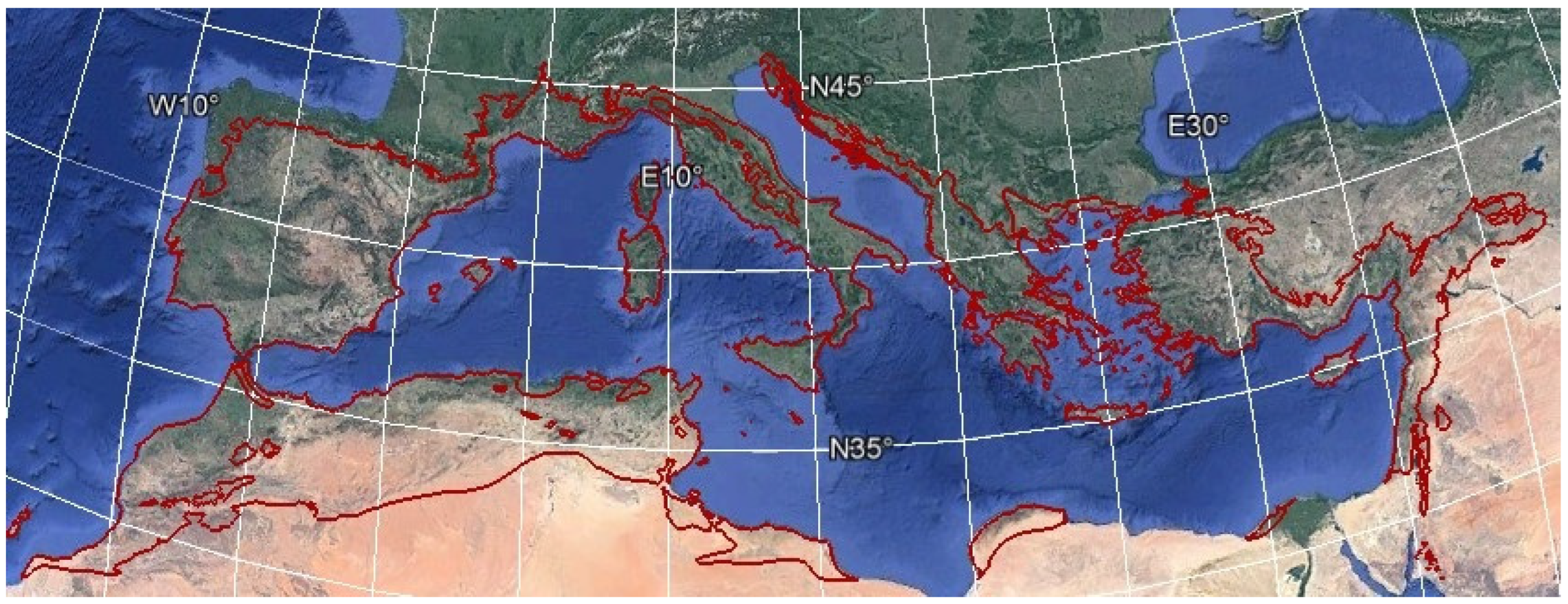
In this study, we defined the Mediterranean region as roughly spanning the area between 10°W–40°E and 30°N–45°N (Figure 1) [41]. The Mediterranean region includes the territories bordering the Mediterranean Sea and specific sets of biogeographical and bioclimatic characteristics distinguish it. Covering an approximate area of 2 million of km² this region is a convergence point for three continents: Europe, Asia, and Africa. The Mediterranean basin is a transition between arid ecosystems located in North Africa and the Near East, and temperate forest ecosystems found in the European mountains. As reported in Köppen–Geiger classification [42], the Mediterranean climate is categorized as a temperate mid-latitude climate with a dry summer season that can be either warm or hot. It is the most extensive among the five regions worldwide that exhibit a Mediterranean-type climate, and the most intricate in terms of geography, encompassing over 40,000 km of rugged coastline that comprises distinct peninsulas and islands [43]. The region hosts a diverse range of plant communities, spanning from Mediterranean evergreen sclerophyllous forests and maquis formations to steppe-like grasslands and coastal dune systems [44]. The Mediterranean Basin shows remarkable landscape heterogeneity, particularly in terms of vegetation, owing to a combination of biogeographic, climatic, and historical factors [45].

2.2. Data Collection and Analysis

2.2.1. Google Earth Engine

The processing and extraction of satellite data were conducted using Google Earth Engine (GEE), which is a vast repository of satellite imagery and geospatial datasets encompassing several petabytes, equipped with the capability to perform analysis on a planetary scale. GEE seamlessly integrates with a high-performance computing service and is accessible through an internet-based application programming interface (API) written in JavaScript, allowing for efficient data analysis and swift visualization of results [46]. This cloud-based spatial analysis platform is freely available to all users, offering a vast array of datasets and algorithms within a unified online environment, significantly reducing data processing times and enhancing computational efficiency. Thanks to the remarkable features of this platform, simultaneous processing of the Landsat-7, Landsat-8 and Sentinel-2 image collections was conducted.

2.2.2. Satellite Data

In this paper, surface reflectance images of Landsat-7, Landsat-8 and Sentinel-2 over the Mediterranean region were used.

The Landsat-7 satellite carries the Enhanced Thematic Mapper Plus (ETM+) sensor. It was launched on 15 April 1999, and provided scientific information for 23 years until 6 April 2022 [47]. The USGS Landsat-7 surface reflectance (SR) product was used (Landsat-7 level 2 collection 2); this dataset contains atmospherically corrected and orthorectified surface reflectance [46,48]. The Landsat-7 SR dataset was developed with the Landsat Ecosystem Disturbance Adaptive Processing System (LEDAPS) algorithm (version 3.4.0) [49]. The Landsat-7 SR data used in this study were archived in GEE as the “LANDSAT/LE07/C02/T1_L2” dataset.

The Landsat-8 satellite carries two sensors on board, the Operational Land Imager (OLI) and the Thermal Infrared Sensor (TIRS), and it was launched on 11 February 2013 [50,51]. The USGS Landsat-8 SR dataset (Landsat-8 level 2 collection 2) which contains atmospherically corrected, orthorectified surface reflectance data was used [46]. Landsat-8 SR products are developed with the Land Surface Reflectance Code (LaSRC) [40,48,52,53]. The Landsat-8 SR data used in this study were archived in GEE as the “LANDSAT/LC08/C02/T1_L2” dataset. Both Landsat-7 and Landsat-8 have a revisit cycle of 16 days.

The Sentinel-2 mission is a constellation of two polar-orbiting satellites that carries Multispectral Instruments (MSI): Sentinel-2A launched on 24 June 2015; Sentinel-2B launched on 7 March 2017 [54]. The combined Sentinel-2 constellation revisit is 5 days. Sentinel-2 MSI surface reflectance data (Sentinel-2, level-2) are generated by the Sen2Cor software [55,56,57].

SR products were preferred to minimize differences due to atmospheric effects [58]. The Sentinel-2 SR data used in this study were archived in GEE as the “COPERNICUS/S2_SR_HARMONIZED” dataset.

Despite the visually similar appearance of the data collected by the sensors, they differ in terms of the number of bands, band centre, bandwidth, and spatial resolution (

Table 1. The nominal band centres, bandwidths, and spatial resolution of Sentinel-2 MSI, Landsat-8 OLI and Landsat-7 ETM+. The asterisk (*) indicates bands that are not assessed in this study. Source of Landsat-7 ETM + and Landsat-8 OLI specifications, USGS (https://earthexplorer.usgs.gov/ (accessed on 2 June 2023)). Sentinel-2 MSI specifications, ESA Copernicus data centre (https://scihub.copernicus.eu/dhus/#/home (accessed on 2 June 2023)).

Sentinel-2/MSI
Band ID	B1 *	B2	B3	B4	B5 *	B6 *	B7	B8	B8A	B9 *	B10 *	B11	B12
Band centre (nm)	442.7	492.4	559.8	664.6	704.1	740	782.8	832.8	864.7	1373.5	945.1	1613.7	2202.4
Nominal bandwidth (nm)	21	66	36	31	15	15	20	106	21	31	20	91	175
Spatial resolution (m)	60	10	10	10	20	20	20	10	20	60	60	20	20
Landsat-8/OLI
Band ID	B1 *	B2	B3	B4	B5	B6	B7	B8 *	NA	B9 *	B10 *	B11 *	NA
Band centre (nm)	443	482.5	562.5	655	865	1610	2200	865	/	1375	10,895	12,005	/
Nominal bandwidth (nm)	20	65	75	50	40	100	200	40	/	30	590	1010	/
Spatial resolution (m)	30	30	30	30	30	30	30	15	/	30	100	100	/
Landsat-7/ETM+
Band ID	B1	B2	B3	B4	B5	B6 *	B7	B8 *	NA	NA	NA	NA	NA
Band centre (nm)	485	560	660	835	1650	11,450	2220	710	/	/	/	/	/
Nominal bandwidth (nm)	70	80	60	130	200	2100	260	380	/	/	/	/	/
Spatial resolution (m)	30	30	30	30	30	60	30	15	/	/	/	/	/

).

Our study was based on the six common bands among the sensors: blue, green, red, near infrared (NIR), shortwave-infrared 1 (SWIR1) and shortwave-infrared 2 (SWIR2) (

Table 2. Nominal spectral band and corresponding band numbers for each sensor. The wavelength ranges (nm) are included in parentheses.

Spectral Band	Sentinel-2	Landsat-8	Landsat-7
Blue	2 (458–522 nm)	2 (450–510 nm)	1 (450–520 nm)
Green	3 (543–578 nm)	3 (530–590 nm)	2 (520–600 nm)
Red	4 (650–680 nm)	4 (640–670 nm)	3 (630–690 nm)
Near Infra-Red (NIR)	8 (785–900 nm)	5 (850–880 nm)	4 (770–900 nm)
	8A (855–875 nm)
Short Wave Infra-Red 1 (SWIR1)	11 (1565–1655 nm)	6 (1570–1650 nm)	5 (1550–1750 nm)
Short Wave Infra-Red 2 (SWIR2)	12 (2100–2280 nm)	7 (2110–2290 nm)	7 (2090–2350 nm)

).

In this paper, we will refer to satellites by using the names of their respective sensors.

2.2.3. Data Processing and Sampling Design

The surface reflectance images were sampled from MSI, OLI and ETM+ sensors lasting from 2017 to 2021. This specific time range was chosen as it represents the last full calendar years in which complete image collections for all three sensors were fully available at the time of the study.

Clouds and cloud shadows can affect the spectral bands and distort their results. Masking was performed using the CFmask algorithm [59,60] for ETM+ and OLI products. The quality assessment band (QA60) in the metadata of Sentinel-2 was used to detect and mask clouds and cloud shadows. The cloudy pixel percentage permitted was less than 20% to minimize cloud and cloud shadow effects.

To facilitate a project that produces 30 m spatial resolution outputs, the last processing step entailed reprojecting all image pairs to the projection and 30-m grid of the initial Landsat OLI image (WGS 84, UTM Zone n—where n denotes the zone number associated with the corresponding Landsat OLI image). To adjust the 10 m and 20 m MSI bands to a 30 m spatial resolution, bicubic interpolation was selected over bilinear or nearest-neighbour interpolation due to its ability to yield a smoother surface. To ensure a comprehensive representation of the variability within the study area, we took into careful consideration both the land cover types and the availability of images for each pairwise comparison.

The final dataset of sampling points was obtained from uniformly distributed random points across each land cover type using the European Space Agency (ESA) “WorldCover” map at 10 m spatial resolution (https://esa-worldcover.org/en (accessed on 2 May 2023)) [61]. The ESA cover map used in this study was archived in GEE as the “ESA/WorldCover/v200”. To meet the requirement for each pairwise comparison in the studied years, the number of observations was increased to 1500 points. This approach ensures a robust and reliable analysis of the area under investigation. The available ETM+, OLI, and MSI values between 2017 and 2021 were extracted for each of these points.

The distinct orbits and swath widths of OLI/ETM+ and MSI sensors facilitate the identification of numerous instances where both satellites capture the same ground locations on the same day. For OLI and ETM+ there are no same-day instances, but instances of 1-day lag were sampled. It is reasonable to assume that there are no significant changes in land surface and atmospheric conditions between the two acquisitions on the same day or adjacent days. Since both satellites are sun-synchronous and have mid-morning overpass time, the pairs of observations are generally only minutes apart, and it can be inferred that no significant changes in land surface occur between the two observations, as demonstrated by Flood (2017) [25].

The pixel values intersecting the sample point location were extracted for the blue, green, red, NIR, SWIR1, and SWIR2 bands for each platform-sensor pair.

To remove any remaining undetected cloud or shadow, the blue band ratio between two sensors (MSI vs. OLI, MSI vs. ETM+, OLI vs. ETM+) was computed. Any data points exhibiting a ratio greater than 2 or less than 0.5 were excluded, on the assumption that these pixels were corresponding to areas that were cloud-free in one image but appeared brighter due to cloud presence or darker due to shadowing in the other image [25]. Following a procedure similar to that reported by Chastain et al. [39], all outlier values beyond four standard deviations were checked and removed (

Table 3. Sample points numbers of each pairwise comparison.

Sensor	Sample Points
MSI vs. OLI	35,234
MSI vs. ETM+	25,880
OLI vs. ETM+	25,640

).

2.3. Method of Analysis

In this study, all sample observations were split into a training (70%) and test (30%) dataset of pairwise pixels (

Table 4. Sample points numbers of each pairwise comparison split into a training and test set.

	Training Set	Test Set
MSI vs. OLI	24,664	10,570
MSI vs. ETM+	18,116	7764
OLI vs. ETM+	17,948	7692

).

Scatterplots were computed to visualize the comparison, where the x-axis stood for the pixel values of Sentinel-2 or Landsat-8 bands, and the y-axis represented the pixel values of Landsat-7 or Landsat-8 bands.

Each scatterplot also displayed the slope of the Orthogonal Distance Regression (ODR) that shows the linear relationship value considering errors in both the independent and dependent variables. The ODR slope measures the change in the dependent variable (e.g., pixel values) for a unit change in the independent variable (e.g., another set of pixel values) in a regression model.

The ODR slope closer to one suggests that the two sets of pixel values have a direct, proportional relationship, where an increase or decrease in one set corresponds to an equal increase or decrease in the other set. It indicates a stronger and more consistent linear relationship between the pixel values.

Two types of regression models were computed to estimate the relationship between the sensor bands: Ordinary Least Squares (OLS) and Major Axis (RMA) regression models. OLS regression models were used to assess the difference between bands for the respective sensors. To fit prediction models, Equation (1) was fitted for each band:

$$p_{xi}=a+b{p}_{xj}$$

(1)

where $p_{xi}$ is the surface reflectance for Landsat 7/8 and Sentinel-2 at a given wavelength, based on the training set pairwise and parameters $a$ and $b$ are intercept and slope applicable to each band, respectively.

The RMA regression model, used by Chastain et al. [39] was also employed to determine the value of differences between each sensor band. Unlike OLS models, RMA assumes that both the dependent and independent variables can be subject to error [62]. This analysis was implemented using the ‘maregress’ function available in MATLAB (https://www.mathworks.com/matlabcentral/fileexchange/27916-maregress (accessed on 5 May 2023)). The regression coefficients (intercept and slope) derived from the two regression models for each band comparison were employed as correction factors for sensor band harmonization, adapting Equation (1), where $p_{xj}$ was replaced with the SR value of the specific band being corrected for each comparison (MSI vs. OLI, MSI vs. ETM+, OLI vs. ETM+). A t-test was used with a significance p-value < 0.05 to assess the relationship between pairs of band reflectance values and determine the accuracy of regression model coefficients. Additionally, two metrics of difference were utilized: the mean difference (Δ) and the root-mean-square deviation (RMSD). The mean difference metric (Equation (2)) provided insights into the average deviation between the predicted and observed reflectance values, indicating systematic bias in the regression model.

$$∆=\sum _i^n\frac{(v_i^a-w_i^b)}{n}$$

(2)

The mean difference represents the arithmetic average of the individual differences between paired values from the two distributions $\left(v_i^a\right)$ and $\left(w_i^b\right)$, capturing the overall directional discrepancy.

RMSD is a statistical measure commonly used in data analysis and computational modelling to quantify the discrepancy or difference between two distributions of data points. It provides a robust estimate of the average deviation or dispersion between corresponding data points, from the two distributions $\left(v_i^a\right)$ and $\left(w_i^b\right)$, respectively (Equation (3)).

$$\mathrm{R}\mathrm{M}\mathrm{S}\mathrm{D}=\sqrt{\frac{1}{N}\sum _i^n\ast {(v_i^a-w_i^b)}^2}$$

(3)

For both metrics, $v_i^a$ and $w_i^b$ vary following the relationship investigated (MSI vs. OLI, MSI vs. ETM+, OLI vs. ETM+).

In the last step, the coefficients obtained for data harmonization were compared with those proposed by Claverie et al. [40] for the NASA HLS product and by Chastain et al. [39] for the CONUS area.

At the time of writing the paper, no harmonization coefficients between the MSI and ETM+ sensors have been released for the NASA HLS product.

The Normalized Difference Vegetation Index (NDVI) for the test dataset pairwise was calculated aiming to compare the reflectance’s value and assess the effectiveness of the correction. It is computed by normalizing the difference between near-infrared and red spectral reflectance for both, harmonized and non-harmonized data. Moreover, NDVI was calculated by using both uncorrected and corrected reflectance values obtained from the OLS and RMA regression models.

3. Results

The results of the conducted analyses are presented to highlight the differences and similarities among the various pairs of sensor surface reflectance values. To better appreciate the differences observed before and after applying the adjusted coefficients, the values related to the analyses conducted on the training sets are reported in the text. These analyses were confirmed and implemented on the test sets, as demonstrated by the results reported in the Appendix A (Appendix A,

Table A1. Statistical differences in surface reflectance between the MSI and OLI band values. Mean difference, and RMSD values for each pairwise band of the test set, comprising a total of 10,570 data points. The asterisk (*) indicates the significance of the t-test, with a p-value < 0.05.

Band	Mean Difference	RMSD
Blue	0.0117 *	0.0207
Green	0.0076 *	0.0194
Red	0.0072 *	0.0194
NIR	0.0025 *	0.0356
NIRa	0.0109 *	0.0367
SWIR1	0.0247 *	0.0443
SWIR2	0.0308 *	0.0456

,

Table A2. Statistical differences in surface reflectance between test set MSI and OLI band values after transformation functions. Mean difference (a) and RMSD values (b) for each pairwise band of the training set subjected to OLS/RMA regression model coefficients in this study, Chastain et al. (2019) and HLS transformation functions (Claverie et al. 2018). The asterisk (*) indicates the significance of the t-test, with a p-value < 0.05. “NA” indicates the absence of a transformation coefficient between band 8 and band 5 of the MSI and OLI sensors, respectively.

(a) Mean Difference MSI vs. OLI Adjusted TEST SET
Band	OLS	RMA	Chastain et al. Coeff.	HLS Coeff.
Blue	1.06 × 10−4	1.68 × 10−4	0.0151 *	0.0057 *
Green	1.91 × 10−4	1.77 × 10−4	0.0044 *	0.0072 *
Red	2.51 × 10−4	−0.0092 *	0.0053 *	0.0106 *
NIR	5.93 × 10−5	−0.0207 *	0.0305 *	NA
NIRa	1.88 × 10−4	6.66 × 10−5	0.0046 *	0.0026 *
SWIR1	1.77 × 10−4	1.90 × 10−4	0.0167 *	0.0249 *
SWIR2	−0.0822 *	1.03 × 10−4	0.0261 *	0.0289 *
(b) RMSD MSI vs. OLI adjusted TEST SET
Band	OLS	RMA	Chastain et al. Coeff.	HLS coeff.
Blue	0.0162	0.0165	0.0222	0.0177
Green	0.0176	0.0177	0.0184	0.0194
Red	0.0225	0.0244	0.0232	0.0256
NIR	0.0354	0.0416	0.0471	NA
NIRa	0.0349	0.0356	0.0356	0.0356
SWIR1	0.0367	0.0371	0.0403	0.0444
SWIR2	0.0935	0.0323	0.0426	0.0443

,

Table A3. Statistical differences in surface reflectance between the MSI and ETM+ band values. Mean difference, and RMSD values for each pairwise band of the test set, comprising a total of 7764 data points. The asterisk (*) indicates the significance of the t-test, with a p-value < 0.05.

Band	Mean Difference	RMSD
Blue	0.0061 *	0.0194
Green	0.0051 *	0.0208
Red	0.0078 *	0.0271
NIR	0.0153 *	0.0421
NIRa	0.0232 *	0.0458
SWIR1	0.0270 *	0.0502
SWIR2	0.0326 *	0.0493

,

Table A4. Statistical differences in surface reflectance between the MSI and ETM+ band values after transformation functions. Mean difference (a) and RMSD values (b) for each pairwise band of the training set subjected to OLS/RMA regression model coefficients in this study and Chastain et al. (2019) transformation functions. The asterisk (*) indicates the significance of the t-test, with a p-value < 0.05.

(a) Mean Difference MSI vs. ETM+ Adjusted TEST SET
Band	OLS	RMA	Chastain et al. Coeff.
Blue	−4.83 × 10−4	−4.38 × 10−4	0.0112 *
Green	−3.51 × 10−4	−3.00 × 10−4	0.0022 *
Red	−4.75 × 10−4	−4.79 × 10−4	0.0006
NIR	−2.15 × 10−4	−3.24 × 10−4	0.0216 *
NIRa	−7.36 × 10−5	−9.69 × 10−5	−0.0061 *
SWIR1	−2.36 × 10−4	−2.56 × 10−4	0.0118 *
SWIR2	−2.49 × 10−4	−2.94 × 10−4	0.0146 *
(b) RMSD MSI vs. ETM adjusted TEST SET
Band	OLS	RMA	Chastain et al. Coeff.
Blue	0.0172	0.0176	0.0206
Green	0.0199	0.0202	0.0203
Red	0.0252	0.0254	0.0252
NIR	0.0392	0.0401	0.0448
NIRa	0.0395	0.0404	0.0426
SWIR1	0.0423	0.0429	0.0443
SWIR2	0.0367	0.0371	0.0395

,

Table A5. Statistical differences in surface reflectance between the OLI and ETM+ band values. Mean difference, and RMSD values for each pairwise band of the test set, comprising a total of 7692 data points. The asterisk (*) indicates the significance of the t-test, with a p-value < 0.05.

Band	Mean Difference	RMSD
Blue	−0.0142 *	0.0188
Green	−0.0132 *	0.0197
Red	−0.0137 *	0.0202
NIR	−0.0063 *	0.0271
NIRa	−0.0162 *	0.0374
SWIR1	−0.0133 *	0.0332
SWIR2	−0.0142 *	0.0188

and

Table A6. Statistical differences in surface reflectance between the OLI and ETM+ band values after transformation functions. Mean difference (a) and RMSD values (b) for each pairwise band of the training set subjected to OLS/RMA regression model coefficients in this study and Chastain et al. (2019) transformation functions. The asterisk (*) indicates the significance of the t-test, with a p-value < 0.05.

(a) Mean Difference OLI vs. ETM+ Adjusted TEST SET
Band	OLS	RMA	Chastain et al. Coeff.
Blue	−1.01 × 10−4	−1.18 × 10−4	−0.0120
Green	−6.78 × 10−5	−1.13 × 10−4	−0.0137
Red	−9.40 × 10−6	−4.98 × 10−5	−0.0186
NIR	−3.36 × 10−4	−2.60 × 10−4	−0.0327
NIRa	−4.07 × 10−4	−3.27 × 10−4	−0.0263
SWIR1	−3.84 × 10−4	−2.95 × 10−4	−0.0296 *
SWIR2	−1.01 × 10−4	−1.18 × 10−4	−0.0120
(b) RMSD OLI vs. ETM adjusted TEST SET
Band	OLS	RMA	Chastain et al. Coeff.
Blue	0.0121	0.0122	0.0175
Green	0.0141	0.0141	0.0202
Red	0.0182	0.0182	0.0276
NIR	0.0261	0.0264	0.0449
NIRa	0.0326	0.0326	0.0443
SWIR1	0.0286	0.0288	0.0448
SWIR2	0.0121	0.0122	0.0175

).

3.1. MSI vs. OLI

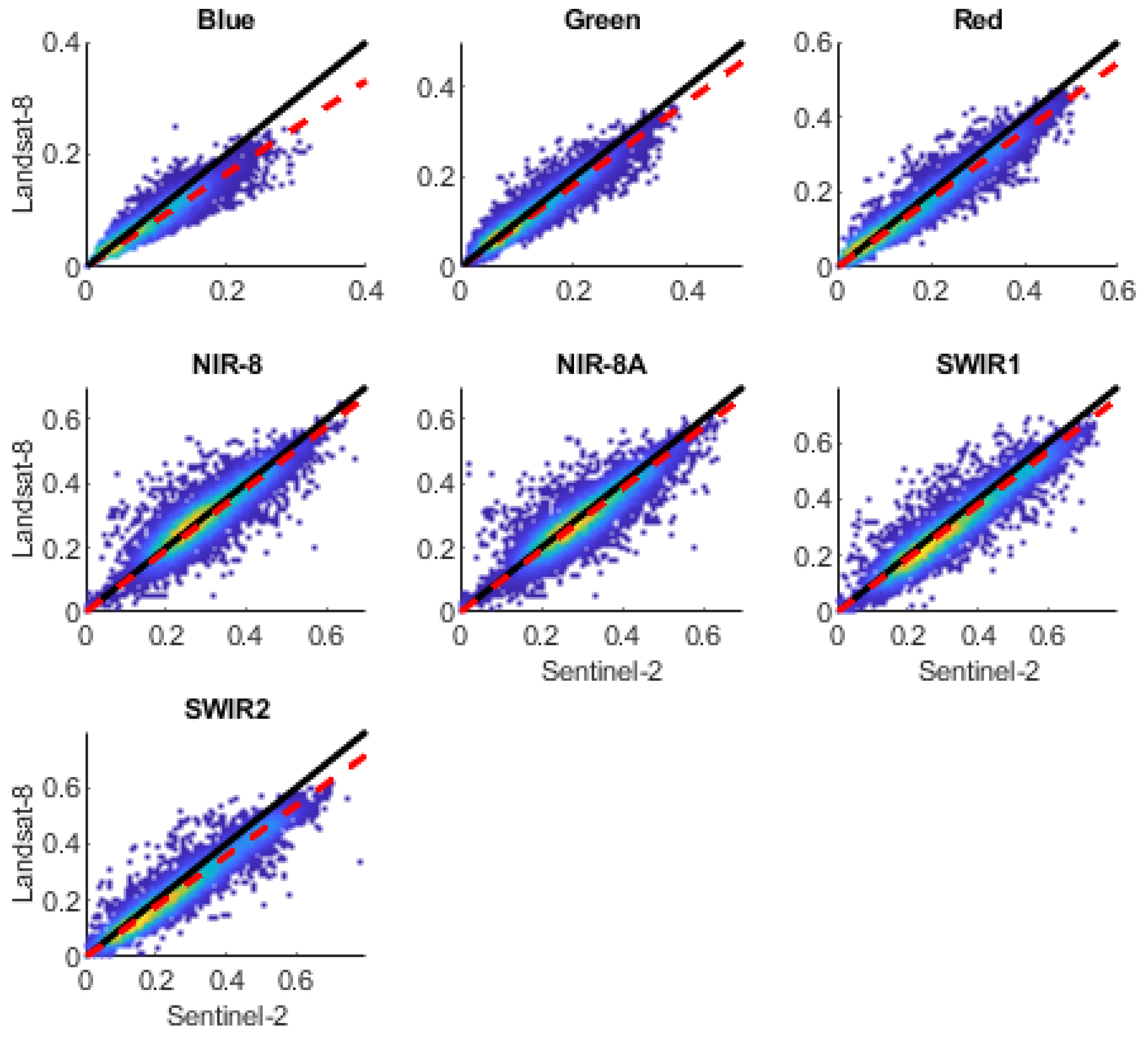
Regarding the comparison of surface reflectance between resampled MSI and OLI pixel values, a reference scatterplot was observed using the training dataset (70%) (Figure 2).

The values exhibit a good level of agreement, as indicated by the dashed line representing the ODR slope, whose values (

Table 5. Statistical differences in surface reflectance between the MSI and OLI band values. ODR slope, mean difference, and RMSD values for each pairwise band of the training set, including a total of 24,664 data points. The asterisk (*) indicates the significance of the t-test, with a p-value < 0.05.

Band	ODR Slope	Mean Difference	RMSD
Blue	0.8284	0.0115 *	0.0206
Green	0.9158	0.0074 *	0.0197
Red	0.9064	0.0122 *	0.0272
NIR	0.9586	0.0025 *	0.0368
NIRa	0.9563	0.0108 *	0.0379
SWIR1	0.9484	0.0246 *	0.0451
SWIR2	0.8958	0.0307 *	0.0464

) are close to 1. The blue band has a higher degree of disagreement (0.8284). Nevertheless, the mean difference values for all bands (Table 5) are statistically significant (p-value < 0.05). The RMSD values (Table 2) range from 0.0197 (Green band) to 0.0464 (SWIR2 band).

Significant differences were identified when adjustment factors found here (

Table 6. Intercept and slope values obtained by applying both OLS and RMA regression models for each pair of MSI surface reflectance as a function of OLI surface reflectance.

Regression Model	Blue	Green	Red	NIR	NIRa	SWIR1	SWIR2
OLS Intercept	0.0016	0.0009	−0.0005	0.0133	0.0204	0.02	0.0113
OLS Slope	1.1297	1.0518	1.0773	0.9637	0.9677	1.0147	1.0829
RMA Intercept	−0.0044	0.0041	0.0047	0.0103	−0.0028	0.0077	0.0035
RMA Slope	1.2071	1.0919	1.1032	1.0432	1.0457	1.0544	1.1163

) were compared with those available in the literature by Chastain et al. [39] and Claverie et al. [40] (

Table 7. Statistical differences in surface reflectance between the training set MSI and OLI band values after transformation functions. Mean difference (a) and RMSD values (b) for each pairwise band of the training set subjected to OLS and RMA regression models in this study and to Chastain et al. [39] and Claverie et al. HLS [40] transformation functions. The asterisk (*) indicates the significance of the t-test, with a p-value < 0.05. “NA” indicates the absence of a transformation coefficient between band 8 and band 5 of the MSI and OLI sensors, respectively.

(a) Mean Difference MSI vs. OLI Adjusted
Band	OLS	RMA	Chastain et al. Coeff.	HLS Coeff.
Blue	−2.54 × 10−5	2.67 × 10−5	0.015 *	0.0055 *
Green	2.78 × 10−5	6.69 × 10−6	0.0043 *	0.0071 *
Red	1.73 × 10−5	−9.42 × 10−3 *	0.0051 *	0.0104 *
NIR	4.81 × 10−5	−2.06 × 10−2 *	0.0304 *	NA
NIRa	−8.24 × 10−3	−8.27 × 10−3	−0.0038 *	0.0026 *
SWIR1	8.04 × 10−7	1.06 × 10−6	0.0165 *	0.0247 *
SWIR2	−8.20 × 10−2 *	4.74 × 10−6	0.0261 *	0.0288 *
(b) RMSD MSI vs. OLI adjusted
Band	OLS	RMA	Chastain et al. Coeff.	HLS Coeff.
Blue	0.0162	0.0165	0.0221	0.0177
Green	0.018	0.0182	0.0187	0.0197
Red	0.023	0.025	0.0237	0.026
NIR	0.0366	0.0426	0.048	NA
NIRa	0.0375	0.0383	0.0372	0.0368
SWIR1	0.0378	0.0382	0.0413	0.0452
SWIR2	0.0938	0.0333	0.0434	0.045

).

The coefficients available in the literature and applied to our dataset revealed statistically significant differences (p-value < 0.05) (Table 7a) for all comparisons between MSI and OLI bands adjusted, with RMSD values (Table 7b) ranging from 0.0187 (green band) to 0.0480 (NIR band) for Chastain et al. (2019) [39] transformation functions, and RMSD values ranging from 0.0177 (blue band) to 0.0452 (SWIR1 band) for the HSL [40] transformation functions.

The regression models developed in this study (OLS and RMA) both improved the fitting of the data for all band pairs (Table 7). The OLS model showed a statistically significant difference only in the SWIR2 band, with RMSD values of 0.0375 and 0.0938, respectively, and a p-value of 2.20 × 10⁻¹⁶. The RMA transformation function showed a statistically significant difference (Table 7a) in the red band (RMSD 0.0250), NIR band (RMSD 0.0426), (Table 7b), with an average p-value of 4.27 × 10⁻²¹. Although some difference values were not significant, an improvement can be observed compared to the initial RMSD values (Table 5). Similarly, for these values, the ODR slope is much closer to the 1-to-1 line (

Table 8. ODR slope values of MSI and OLI comparison after transformation function application.

MSI vs. OLI ODR Adjusted
Band	OLS	RMA
Blue	0.9424	1.0108
Green	0.9649	1.0030
Red	0.9781	1.0021
NIR	0.9211	1.0034
NIRa	0.9231	1.0035
SWIR1	0.9629	1.0020
SWIR2	1.0262	1.0031

).

3.2. MSI vs. ETM+

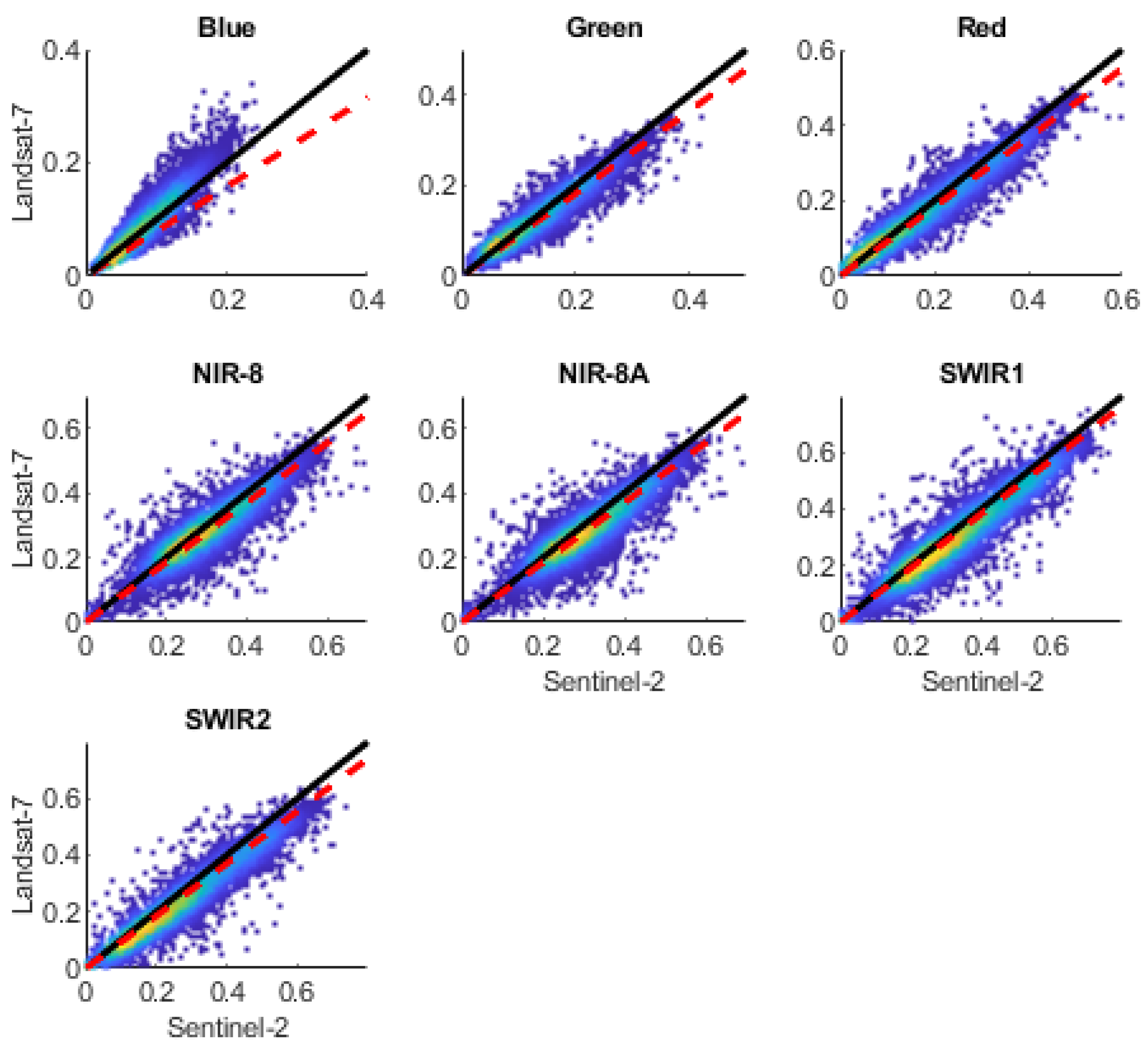
The scatterplot representing the comparison between paired surface reflectance pixel values of satellites Sentinel-2 and Landsat-7 (training dataset) was reported in Figure 3. This comparison between sensors also demonstrates a good level of agreement, as evidenced by the dashed line representing the ODR slope values (Figure 3;

Table 9. Statistical differences in surface reflectance between the MSI and ETM+ band values. ODR slope, mean difference, and RMSD values for each pairwise band of the training set, comprising a total of 18,116 data points. The asterisk (*) indicates the significance of the t-test, with a p-value < 0.05.

Band	ODR Slope	Mean Difference	RMSD
Blue	0.7901	0.0065 *	0.0196
Green	0.9119	0.0055 *	0.0210
Red	0.9164	0.0083 *	0.0274
NIR	0.9243	0.0156 *	0.0422
NIRa	0.9238	0.0232 *	0.0457
SWIR1	0.9564	0.0273 *	0.0505
SWIR2	0.9251	0.0329 *	0.0498

).

The blue band has a higher degree of disagreement (ODR slope, 0.7901).

Nevertheless, the mean difference values for all band comparisons are statistically significant (p-value < 0.05) and the RMSD values range from 0.0196 (Blue band) to 0.0505 (SWIR1 band) (Table 9).

Applying adjustment coefficients of the regression models from this study (OLS/RMA) (

Table 10. Intercept and slope values obtained by applying both OLS and RMA regression models for each pair of MSI surface reflectance as a function of ETM+ surface reflectance.

Regression Model	Blue	Green	Red	NIR	NIRa	SWIR1	SWIR2
OLS Intercept	−0.0083	−0.0037	−0.0041	0.0065	0.0038	0.0067	−0.0083
OLS Slope	0.9375	0.934	0.9325	0.959	0.9416	0.9246	0.9375
RMA Intercept	−0.0119	−0.0067	−0.0067	−0.0063	−0.0054	0.0010	−0.0119
RMA Slope	0.9764	0.9554	0.9464	1.0009	0.9688	0.9462	0.9764

) and those available in the literature, by Chastain et al. [39], statistical differences were appreciated (

Table 11. Statistical differences in surface reflectance between the MSI and ETM+ band values after transformation functions. Mean difference (a) and RMSD values (b) for each pairwise band of the training set subjected to OLS and RMA regression models in this study and to Chastain et al. [39] transformation functions. The asterisk (*) indicates the significance of the t-test, with a p-value < 0.05.

(a) Mean Difference MSI vs. ETM+ Adjusted
Band	OLS	RMA	Chastain et al. Coeff.
Blue	−7.68 × 10−6	4.40 × 10−5	0.0116 *
Green	1.91 × 10−6	4.54 × 10−5	0.0026 *
Red	4.62 × 10−6	−1.05 × 10−5	0.001
NIR	3.68 × 10−5	−1.24 × 10−5	0.0219 *
NIRa	−5.09 × 10−5	−1.40 × 10−5	−0.006 *
SWIR1	6.16 × 10−5	4.80 × 10−5	0.0121 *
SWIR2	3.66 × 10−5	−3.22 × 10−5	0.0149 *
(b) RMSD MSI vs. ETM+ adjusted
Band	OLS	RMA	Chastain et al. Coeff.
Blue	0.0172	0.0176	0.0209
Green	0.0201	0.0204	0.0206
Red	0.0253	0.0255	0.0253
NIR	0.0392	0.0401	0.0449
NIRa	0.0394	0.0404	0.0426
SWIR1	0.0425	0.043	0.0445
SWIR2	0.0369	0.0373	0.0398

).

The coefficients available in the literature and applied to our dataset revealed statistically significant differences (p-value < 0.05) (Table 11a) for all comparisons between MSI and ETM+ bands adjusted, except for the red band. RMSD values (Table 11b) range from 0.0026 (green band) to 0.0449 (NIR band) for Chastain et al. [39] transformation functions.

The regression models developed in this study (OLS and RMA) both improved the fitting of the data for all band pairs (Table 11). No statistically significant difference was revealed by the t-test p-value. An improvement can be observed compared to the initial RMSD values (Table 9) and post-transformation RMSD values; those range from 0.0172 (blue band) to 0.0425 (SWIR1 band), and from 0.0176 (blue band) to 0.0430 (SWIR1 band) following the OLS and RMA transformation functions, respectively.

At the same time, the post-transformed ODR slope is much closer to the 1-to-1 line (

Table 12. ODR slope values of MSI and ETM+ comparison after transformation function application.

MSI vs. ETM+ ODR Adjusted
Band	OLS	RMA
Blue	0.9339	1.0155
Green	0.9555	1.0041
Red	0.9734	1.0023
NIR	0.9134	1.0068
NIRa	0.9124	1.0070
SWIR1	0.9542	1.0020
SWIR2	0.9658	1.0026

) with respect to the initial value (Table 9).

3.3. OLI vs. ETM+

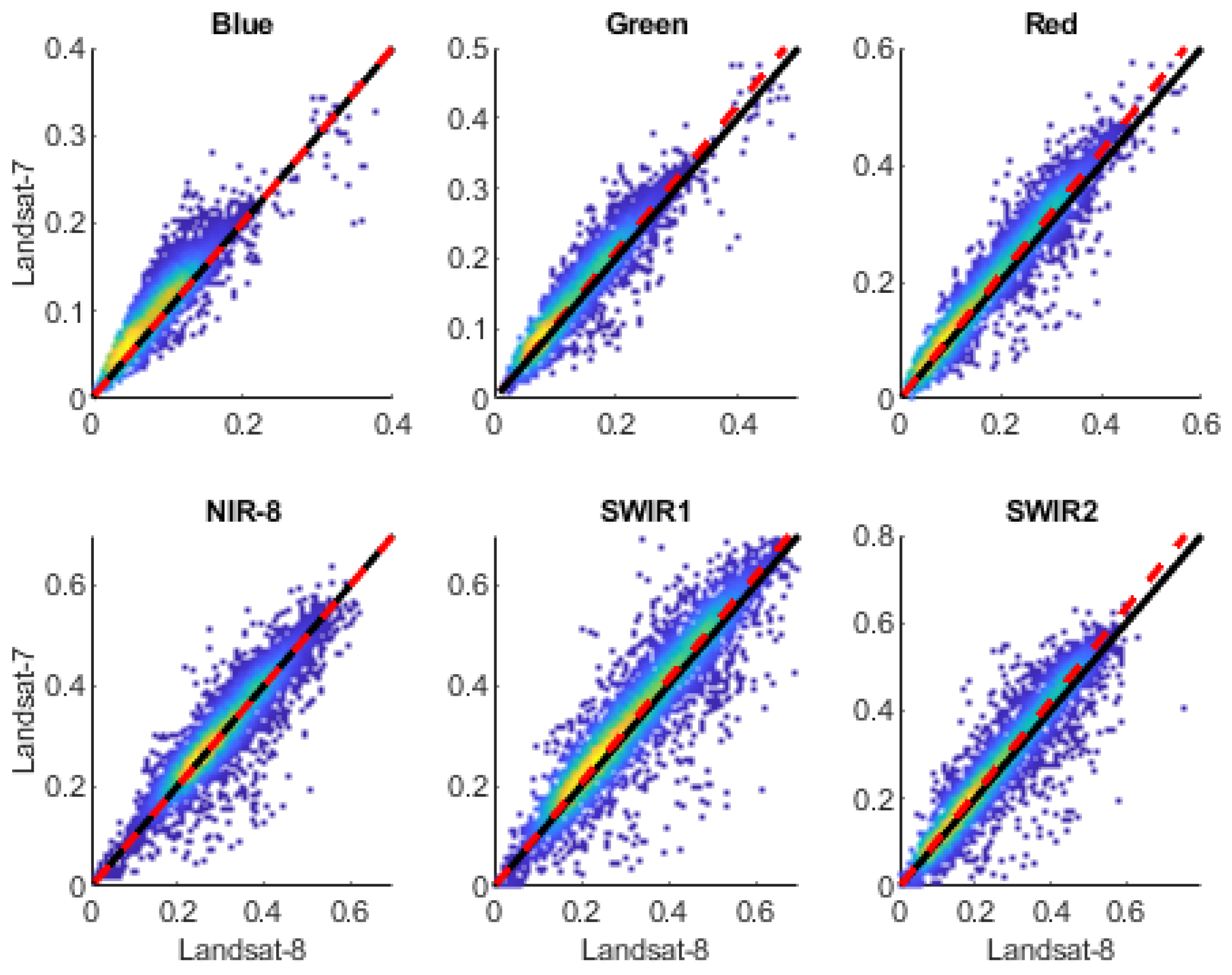
The scatterplot standing for the comparison between paired surface reflectance pixel values of satellites Landsat-8 and Landsat-7 (training dataset) was reported in Figure 4. This inter-comparison between sensors has the best grade of agreement, as evidenced by the dashed line representing the ODR slope values which—in some cases—coincides with the 1-to-1 line (Blue band) (Figure 4;

Table 13. Statistical differences in surface reflectance between the OLI and ETM+ band values. ODR slope, mean difference, and RMSD values for each pairwise band of the training set, comprising a total of 25,640 data points. The asterisk (*) indicates the significance of the t-test, with a p-value < 0.05.

Band	ODR Slope	Mean Difference	RMSD
Blue	1.0026	−0.0141 *	0.0186
Green	1.0467	−0.0131 *	0.0196
Red	1.0566	−0.0169 *	0.0256
NIR	0.9992	−0.0060 *	0.0267
SWIR1	1.0322	−0.0159 *	0.0366
SWIR2	1.0569	−0.0130 *	0.0327

). The NIR band has the higher degree of disagreement (0.9992).

The mean difference values for all band comparisons (Table 13) are statistically significant (p-value < 0.05). The RMSD values range from 0.0186 (Blue band) to 0.0366 (SWIR1 band).

A statistical difference was observed applying adjustment coefficients of the regression models from this study (OLS/RMA) (

Table 14. Intercept and slope values obtained by applying both OLS and RMA regression models for each pair of OLI surface reflectance as a function of ETM+ surface reflectance.

Regression Model	Blue	Green	Red	NIR	SWIR1	SWIR2
OLS Intercept	−0.0083	−0.0037	−0.0041	0.0065	0.0038	0.0067
OLS Slope	0.9375	0.934	0.9325	0.959	0.9416	0.9246
RMA Intercept	−0.0119	−0.0067	−0.0067	−0.0063	−0.0054	0.0010
RMA Slope	0.9764	0.9554	0.9464	1.0009	0.9688	0.9462

) and those available in the literature by Chastain et al. [39].

The coefficients available in the literature and applied to our dataset revealed statistically significant differences (p-value < 0.05) (

Table 15. Statistical differences in surface reflectance between the OLI and ETM+ band values after transformation functions. Mean difference (a) and RMSD values (b) for each pairwise band of the training set subjected to OLS and RMA regression models in this study and to the Chastain et al. [39] transformation functions. The asterisk (*) indicates the significance of the t-test, with a p-value < 0.05.

(a) Mean Difference OLI vs. ETM+ Adjusted
Band	OLS	RMA	Chastain et al. Coeff.
Blue	1.06 × 10−7	4.88 × 10−6	−0.0118 *
Green	−5.29 × 10−7	−3.68 × 10−5	−0.0136 *
Red	3.49 × 10−5	−4.85 × 10−6	−0.0186 *
NIR	−1.80 × 10−5	1.49 × 10−5	−0.0326 *
SWIR1	−5.56 × 10−5	3.79 × 10−6	−0.026 *
SWIR2	−3.72 × 10−5	4.33 × 10−5	−0.0293 *
(b) RMSD OLI vs. ETM+ adjusted
Band	OLS	RMA	Chastain et al. Coeff.
Blue	0.0119	0.012	0.0173
Green	0.0139	0.0139	0.02
Red	0.0179	0.0179	0.0274
NIR	0.0258	0.026	0.0446
SWIR1	0.0319	0.0321	0.0435
SWIR2	0.0282	0.0284	0.0442

a) for all comparisons between OLI and ETM+ bands adjusted, RMSD ranging from 0.0173 (blue band) to 0.0446 (NIR band) for Chastain et al. (2019) [39] transformation functions (Table 15b).

The regression models developed in this study (OLS and RMA) both improved the fitting of the data for all band pairs (Table 15). No statistically significant difference was revealed by the t-test p-value. An improvement can be observed compared to the initial RMSD values (Table 13) and post-transformation RMSD values (Table 15). The RMSD range is very similar to the results obtained from the application of transformation coefficients of both regression models (OLS, RMA). The RMSD ranges from 0.12 for the blue band to 0.028 for the SWIR2 band.

The post-transformed ODR slope values did not show significant changes, as the original values were already very close to the 1-to-1 line (Appendix B,

Table A7. ODR slope values of OLI and ETM+ comparison after transformation function application.

OLI vs. ETM ODR Adjusted
Band	OLS	RMA
Blue	1.0026	1.0026
Green	0.9760	0.9989
Red	0.9842	0.9999
NIR	0.9564	1.0001
SWIR1	0.9701	0.9990
SWIR2	0.9753	0.9986

).

3.4. NDVI Computation

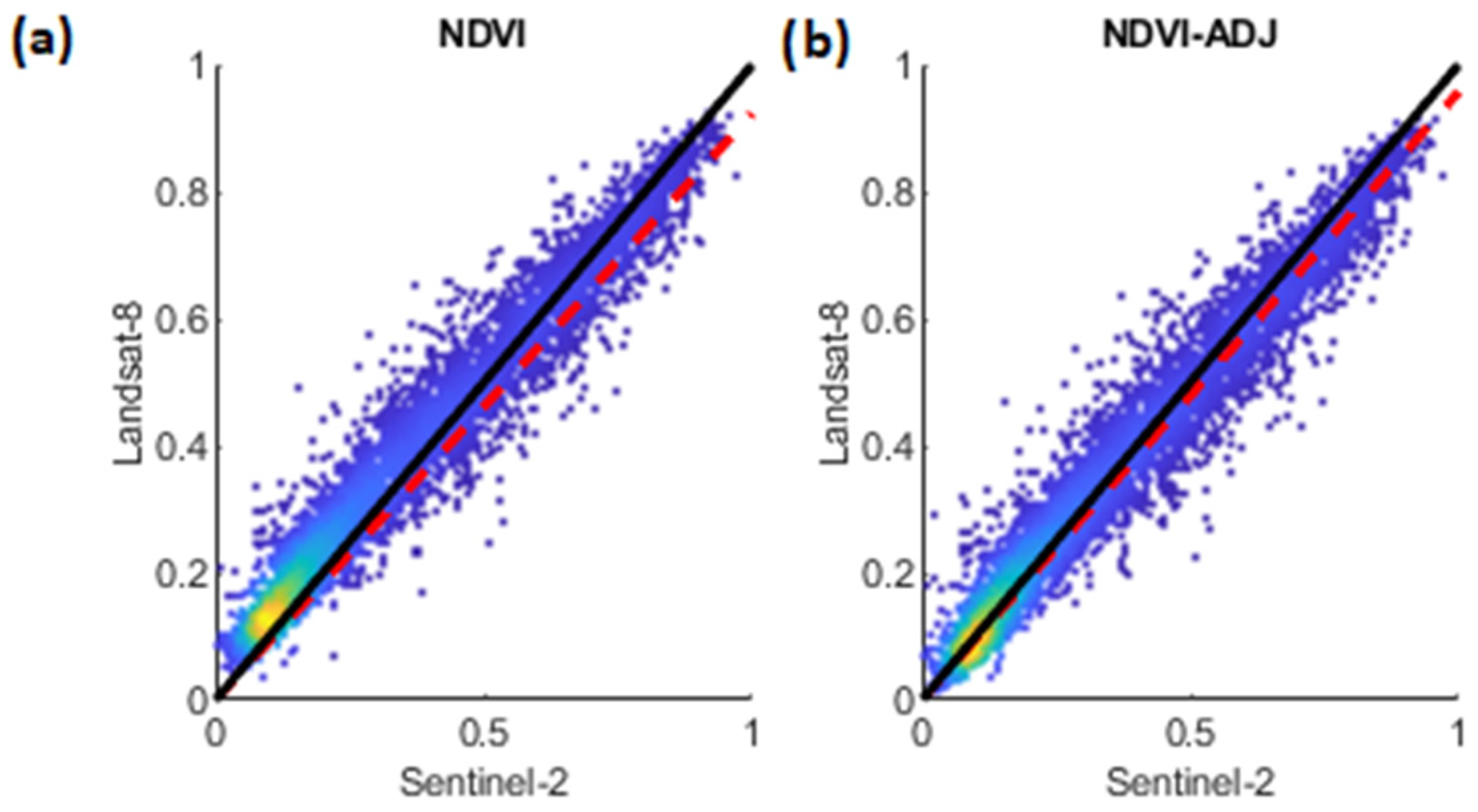
Figure 5 presents a comparison between NDVI computed from MSI and OLI sensors on the test set (10,570 pairwise samples). Specifically, it reports the comparison between the sensor value pairs before applying adjustment coefficients. The orthogonal distance regression (ODR) slope is measured at 0.92, and the mean difference with a value of −0.0243 shows statistical significance (t-test, p-value 1.63 × 10⁻¹⁴). Additionally, the Root-Mean-Square Deviation (RMSD) is computed to be 0.050 (Figure 5a).

The same comparison is made after applying the adjustment factors from the OLS model in Table 6 (Figure 5b). The ODR slope has increased to 0.95, and the mean difference, with a value of −0.0211, is no longer statistically significant (t-test, p-value 0.7204). The RMSD remains unchanged. The comparison with Landsat-7 is omitted for brevity; however, it exhibits very similar behaviour to the previous comparisons.

4. Discussion

This study aims to assess the differences and propose cross-sensor conversion factors derived from the integrated or exclusive use of OLS and RMA regression models between Landsat-7, Landsat-8, and Sentinel-2 surface reflectance products. The objective is to take advantage of the potential arising from the harmonization of these products. While the previous literature has primarily focused on integrating TOA reflectance products in different areas, this study, for the first time, concentrates on the highly heterogeneous Mediterranean Basin using surface reflectance products, representing a significant advancement in the integration of satellite products within this region.

Despite the good agreement observed in the comparison (Figure 2 and Figure 3) between Landsat-7/8 and Sentinel-2 products, significant variations exist between cross-sensor band pairs, as demonstrated by mean differences and RMSD (Table 5, Table 9 and Table 13). The slope of the ODR shows equivalent results for MSI vs. OLI (Table 5) and MSI vs. ETM+ (Table 9) comparisons, with values close to 1 for the visible bands, particularly the blue band. A higher disagreement was observed for the blue band between the MSI vs. ETM+ sensor pairs where a notable mismatched band width was reported (Table 2). In the case of the NIR band, MSI bands 8 and 8a exhibit remarkably similar ODR slopes and RMSD values when compared to OLI and ETM+ bands 5 and 4, respectively. For the comparison between Landsat 7/8 and Sentinel-2 the greatest deviation (RMSD) is observed in the SWIR bands. The SWIR1 (wavelength range 1565–1655 nm) and SWIR2 (wavelength range) bands of MSI exhibit greater deviation compared to the SWIR bands of ETM+ (SWIR1: wavelength range 1570–1750 nm, SWIR2: wavelength range 2090–2350 nm) with respect to the OLI ones (SWIR1: wavelength range 1570–1650 nm, SWIR2: wavelength range 2110–2290 nm). Overall, the RMSD resulting from the MSI vs. ETM+ comparison is higher than the RMSD of MSI vs. OLI.

As expected, the comparison between sensors from the same satellite family (OLI vs. ETM+) shows a higher degree of agreement, as confirmed by the ODR slope, which is still close to 1 (Table 13). In this case as well, the greatest RMSD is observed in the SWIR bands, despite slight differences in the wavelength range (Table 2). The comparison analysis between the bands of different sensors, supported by the calculated difference metrics, suggests that despite a general good level of agreement, the differences in the recorded values are statistically significant. Therefore, for the integrated use of the three sensors in the Mediterranean basin area, calibration and harmonization are necessary.

This study presents the results of two regression models, OLS, and RMA, suggesting a mixed band adjustment based on the coefficients of both models and supported by statistical analyses. Taking into consideration the RMSD, the mean difference and the ODR slope values, integrating the coefficients of the two models is suggested for band adjustment. For the harmonization between OLI and MSI bands, integrating the use of RMA coefficients for Blue, Green, NIRa, SWIR1 and SWIR2 bands, and OLS coefficients for Red and NIR bands, is suggested. For the harmonization between ETM+ and MSI bands, integrating the use of RMA coefficients for Blue and SWIR1 bands, and OLS coefficients for Red, NIR, Green, NIRa and SWIR2 bands, is suggested. Finally, for the harmonization between ETM+ and OLI bands, integrating the use of RMA coefficients for Red, NIR and SWIR2 bands, and OLS coefficients for Blue, Green and SWIR1 bands, is suggested. However, this approach is not mandatory, as shown in the results tables (Table 7, Table 11 and Table 15), where both models improve sensor calibration. Application of the proposed coefficients significantly enhances the agreement between sensors, as demonstrated by the calculation of NDVI. The NDVI comparison obtained after the band correction proposed shows a slight improvement in mean difference value. It is important to underline that following the adjustment, the difference between the variables decreased to such an extent that it was not statistically significant. Finally, the ODR analysis shows a better agreement between the variables, although the RMSD does not significantly change its value. This observation could be attributed to the NDVI equation; it is obtained from the normalized difference between NIR and RED bands, which does not exhibit a higher degree of disagreement between sensor pairs. It is expected that more complex indices, incorporating other spectral bands, may reinforce these findings. The use of coefficients for sensor calibration is strongly recommended, not only for long-term historical analysis but also to increase data frequency, which is crucial in land cover change analyses, and to overcome issues caused by clouds and shadows [28]. Large-scale studies underline the importance and potential of site-specific harmonization models, as observed by Flood et al. in Australia [25] and by Cao et al. in China [26]. These studies reveal that variations between SR values due to sensor differences are significant when comparing different satellite products, and each region is characterized by distinct variations in these values. Similar findings have been confirmed in this study within the Mediterranean basin area, where discrepancies in SR values were bridged through appropriate site-specific harmonization coefficients. The validity and utility of these coefficients were confirmed through conducted statistical analyses and comparisons with coefficients already reported in the literature [39,40]. As demonstrated in all the regional-scale studies presented in this work [25,26,39,40], the integration of long-time-series reflectance values and numerous sampling points distributed throughout the area of interest enables the creation of a highly robust experimental design. This work, for the first time, integrates the SR values from the MSI, OLI, and ETM+ sensors for all overlapping years (2017–2021) using a dataset of sample points that encompasses a wide range of reflectance variability in the Mediterranean basin. This integration significantly reinforces the reliability of the harmonization method. Several studies conducted in smaller areas within the Mediterranean basin have emphasized the need to thoroughly evaluate potential integration between satellite products [63,64]. Others, like Lessio et al. [38], have highlighted how differences in satellite reflectance values can adversely impact the assessment of time series for biophysical variables, often leading to an overestimation of them.

However, previous workflow harmonization efforts have been limited to local scales, as seen in the work by Mandanici et al. [65], resulting in coefficients with limited generalizability. This study addresses this literature gap by being the only work to harmonize different sensors within the Mediterranean basin and being the sole harmonization study at a regional scale in Europe. Given these insights, the process of harmonizing satellite products from the MSI, OLI, and ETM+ sensors in the Mediterranean basin, characterized by specific bioclimatic and biogeographic features, serves as an excellent test site for obtaining harmonization coefficients that encapsulate a unique variability, making it valuable for future research. In conclusion, the difference between the results obtained using the coefficients in this study and those proposed from the literature could be attributed to the sampling method. The work by Claverie et al. [40] on the HLS product was based on a global dataset with few sampled points in the Mediterranean Basin, while Chastain et al. (2019) [39] proposed a method based on points sampled in the CONUS region. Another explanation could be attributed to different techniques for transforming surface reflectance, which is why the authors of this study chose to utilize a pre-existing surface reflectance product available in the GEE library to avoid such issues for users [66].

5. Conclusions

The results obtained from this study aim to provide a harmonization procedure that allows for expanding the availability of comparable surface reflectance data for the Mediterranean basin area. The analysis of surface reflectance products demonstrates a good level of agreement, but the conducted analyses and comparisons with existing studies in the literature have highlighted the potential of integrating the available products with site-specific transformation factors.

Satellite data processing was conducted using open-source software GEE, a cloud-based platform that provides freely accessible surface reflectance datasets. The use of GEE made it possible to analyse and process the large geospatial datasets used in this study, which would have otherwise required significant computing and storage capacity. Working directly with the collections of the three sensors online through GEE’s library eliminated the need to download satellite images separately. The ability to post-process entire image collections simultaneously, extract values, and apply harmonization coefficients using GEE’s API makes the data used in this study easily analysable. Additionally, the use of atmospherically corrected products already available in GEE for all the sensors investigated facilitates the methodology’s application even for users with limited experience in remote-sensing techniques. These characteristics ensure the reproducibility of the methodological approach and enable its widespread application to other studies in the Mediterranean basin area.

The application of this experimental design encountered difficulties primarily due to the limited availability of disturbance-free images (clouds, shadows), necessitating an increase in sampling points and longer computational times, as well as a need for a reliable internet connection.

The authors did not apply BRDF and haze corrections since the aim of the study was to develop band-wise correction factors applicable to a broad range of users. It is assumed that the application of such corrections could further enhance the results already obtained in this study. The future challenge will undoubtedly involve integrating these corrections into the proposed model and assessing their contribution.

References

1. Lechner, A.M.; Foody, G.M.; Boyd, D.S. Applications in Remote Sensing to Forest Ecology and Management. One Earth 2020, 2, 405–412. [Google Scholar] [CrossRef]
2. Wulder, M.A.; Masek, J.G.; Cohen, W.B.; Loveland, T.R.; Woodcock, C.E. Opening the Archive: How Free Data Has Enabled the Science and Monitoring Promise of Landsat. Remote Sens. Environ. 2012, 122, 2–10. [Google Scholar] [CrossRef]
3. Gómez, C.; White, J.C.; Wulder, M.A. Optical Remotely Sensed Time Series Data for Land Cover Classification: A Review. ISPRS J. Photogramm. Remote Sens. 2016, 116, 55–72. [Google Scholar] [CrossRef] [Green Version]
4. Gao, L.; Wang, X.; Johnson, B.A.; Tian, Q.; Wang, Y.; Verrelst, J.; Mu, X.; Gu, X. Remote Sensing Algorithms for Estimation of Fractional Vegetation Cover Using Pure Vegetation Index Values: A Review. ISPRS J. Photogramm. Remote Sens. 2020, 159, 364–377. [Google Scholar] [CrossRef]
5. Segarra, J.; Buchaillot, M.L.; Araus, J.L.; Kefauver, S.C. Remote Sensing for Precision Agriculture: Sentinel-2 Improved Features and Applications. Agronomy 2020, 10, 641. [Google Scholar] [CrossRef]
6. Omia, E.; Bae, H.; Park, E.; Kim, M.S.; Baek, I.; Kabenge, I.; Cho, B.-K. Remote Sensing in Field Crop Monitoring: A Comprehensive Review of Sensor Systems, Data Analyses and Recent Advances. Remote Sens. 2023, 15, 354. [Google Scholar] [CrossRef]
7. Majasalmi, T.; Rautiainen, M. The Potential of Sentinel-2 Data for Estimating Biophysical Variables in a Boreal Forest: A Simulation Study. Remote Sens. Lett. 2016, 7, 427–436. [Google Scholar] [CrossRef]
8. Banskota, A.; Kayastha, N.; Falkowski, M.J.; Wulder, M.A.; Froese, R.E.; White, J.C. Forest Monitoring Using Landsat Time Series Data: A Review. Can. J. Remote Sens. 2014, 40, 362–384. [Google Scholar] [CrossRef]
9. Wang, L.; Jia, M.; Yin, D.; Tian, J. A Review of Remote Sensing for Mangrove Forests: 1956–2018. Remote Sens. Environ. 2019, 231, 111223. [Google Scholar] [CrossRef]
10. Cavender-Bares, J.; Schneider, F.D.; Santos, M.J.; Armstrong, A.; Carnaval, A.; Dahlin, K.M.; Fatoyinbo, L.; Hurtt, G.C.; Schimel, D.; Townsend, P.A.; et al. Integrating Remote Sensing with Ecology and Evolution to Advance Biodiversity Conservation. Nat. Ecol. Evol. 2022, 6, 506–519. [Google Scholar] [CrossRef]
11. Sepuru, T.K.; Dube, T. An Appraisal on the Progress of Remote Sensing Applications in Soil Erosion Mapping and Monitoring. Remote Sens. Appl. Soc. Environ. 2018, 9, 1–9. [Google Scholar] [CrossRef]
12. Zhang, X. Reconstruction of a Complete Global Time Series of Daily Vegetation Index Trajectory from Long-Term AVHRR Data. Remote Sens. Environ. 2015, 156, 457–472. [Google Scholar] [CrossRef]
13. Tan, B.; Morisette, J.T.; Wolfe, R.E.; Gao, F.; Ederer, G.A.; Nightingale, J.; Pedelty, J.A. An Enhanced TIMESAT Algorithm for Estimating Vegetation Phenology Metrics from MODIS Data. IEEE J. Sel. Top. Appl. Earth Obs. Remote Sens. 2011, 4, 361–371. [Google Scholar] [CrossRef]
14. Li, S.; Xu, L.; Jing, Y.; Yin, H.; Li, X.; Guan, X. High-Quality Vegetation Index Product Generation: A Review of NDVI Time Series Reconstruction Techniques. Int. J. Appl. Earth Obs. Geoinf. 2021, 105, 102640. [Google Scholar] [CrossRef]
15. Walther, G.-R.; Post, E.; Convey, P.; Menzel, A.; Parmesan, C.; Beebee, T.J.C.; Fromentin, J.-M.; Hoegh-Guldberg, O.; Bairlein, F. Ecological Responses to Recent Climate Change. Nature 2002, 416, 389–395. [Google Scholar] [CrossRef]
16. Kelly, A.E.; Goulden, M.L. Rapid Shifts in Plant Distribution with Recent Climate Change. Proc. Natl. Acad. Sci. USA 2008, 105, 11823–11826. [Google Scholar] [CrossRef]
17. Reichstein, M.; Bahn, M.; Ciais, P.; Frank, D.; Mahecha, M.D.; Seneviratne, S.I.; Zscheischler, J.; Beer, C.; Buchmann, N.; Frank, D.C.; et al. Climate Extremes and the Carbon Cycle. Nature 2013, 500, 287–295. [Google Scholar] [CrossRef]
18. Zhou, L.; Tian, Y.; Myneni, R.B.; Ciais, P.; Saatchi, S.; Liu, Y.Y.; Piao, S.; Chen, H.; Vermote, E.F.; Song, C.; et al. Widespread Decline of Congo Rainforest Greenness in the Past Decade. Nature 2014, 509, 86–90. [Google Scholar] [CrossRef]
19. Wu, D.; Zhao, X.; Liang, S.; Zhou, T.; Huang, K.; Tang, B.; Zhao, W. Time-Lag Effects of Global Vegetation Responses to Climate Change. Glob. Chang. Biol. 2015, 21, 3520–3531. [Google Scholar] [CrossRef]
20. Li, J.; Roy, D. A Global Analysis of Sentinel-2A, Sentinel-2B and Landsat-8 Data Revisit Intervals and Implications for Terrestrial Monitoring. Remote Sens. 2017, 9, 902. [Google Scholar] [CrossRef] [Green Version]
21. Nikolakopoulos, K.G.; Papoulis, D. A Preliminary Comparison between Landsat-8 OLI and Sentinel-2 MSI for Geological Applications. In Living Planet Symposium, Proceedings of the Conference Held in Prague, Czech Republic, 9–13 May 2016; Ouwehand, L., Ed.; ESA-SP: São Paulo, Brazil, 2016; Volume 740, p. 203. ISBN 978-92-9221-305-3. [Google Scholar]
22. Mantas, V.M.; Marques, J.C.; Pereira, A.J.S.C. A Data Fusion Approach for the Production of Impervious Surface Area Estimates Using Sentinel-1 A and Landsat-8 Data. In Living Planet Symposium, Proceedings of the Conference Held in Prague, Czech Republic, 9–13 May 2016; Ouwehand, L., Ed.; ESA-SP: São Paulo, Brazil, 2016; Volume 740, p. 112. ISBN 978-92-9221-305-3. [Google Scholar]
23. Li, Z.; Xu, D.; Guo, X. Remote Sensing of Ecosystem Health: Opportunities, Challenges, and Future Perspectives. Sensors 2014, 14, 21117–21139. [Google Scholar] [CrossRef] [Green Version]
24. Lefebvre, A.; Sannier, C.; Corpetti, T. Monitoring Urban Areas with Sentinel-2A Data: Application to the Update of the Copernicus High Resolution Layer Imperviousness Degree. Remote Sens. 2016, 8, 606. [Google Scholar] [CrossRef] [Green Version]
25. Flood, N. Comparing Sentinel-2A and Landsat 7 and 8 Using Surface Reflectance over Australia. Remote Sens. 2017, 9, 659. [Google Scholar] [CrossRef] [Green Version]
26. Cao, H.; Han, L.; Li, L. Harmonizing Surface Reflectance between Landsat-7 ETM+, Landsat-8 OLI, and Sentinel-2 MSI over China. Environ. Sci. Pollut. Res. 2022, 29, 70882–70898. [Google Scholar] [CrossRef]
27. Xiong, S.; Du, S.; Zhang, X.; Ouyang, S.; Cui, W. Fusing Landsat-7, Landsat-8 and Sentinel-2 Surface Reflectance to Generate Dense Time Series Images with 10 m Spatial Resolution. Int. J. Remote Sens. 2022, 43, 1630–1654. [Google Scholar] [CrossRef]
28. Senf, C.; Leitão, P.J.; Pflugmacher, D.; van der Linden, S.; Hostert, P. Mapping Land Cover in Complex Mediterranean Landscapes Using Landsat: Improved Classification Accuracies from Integrating Multi-Seasonal and Synthetic Imagery. Remote Sens. Environ. 2015, 156, 527–536. [Google Scholar] [CrossRef]
29. Adrian, R.; Gerten, D.; Huber, V.; Wagner, C.; Schmidt, S.R. Windows of Change: Temporal Scale of Analysis Is Decisive to Detect Ecosystem Responses to Climate Change. Mar. Biol. 2012, 159, 2533–2542. [Google Scholar] [CrossRef]
30. Vafeidis, A.T.; Abdulla, A.A.; Bondeau, A.; Brotons, L.; Ludwig, R.; Portman, M.; Reimann, L.; Vousdoukas, M.; Xoplaki, E. Managing Future Risks and Building Socioecological Resilience. In Climate and Environmental Hange in the Mediterranean Basin—Current Situation and Risks for the Future; First Mediterranean Assessment Report; Union for the Mediterranean, Plan Bleu, UNEP/MAP: Marseille, France, 2021. [Google Scholar] [CrossRef]
31. Appiagyei, B.D.; Belhoucine-Guezouli, L.; Bessah, E.; Morsli, B.; Fernandes, P.A.M. A Review on Climate Change Impacts on Forest Ecosystem Services in the Mediterranean Basin. J. Landsc. Ecol. 2022, 15, 1–26. [Google Scholar] [CrossRef]
32. Noce, S.; Santini, M. Mediterranean Forest Ecosystem Services and Their Vulnerability; Foundation Euro-Mediterranean Center on Climate Change (CMCC): Viterbo, Italy, 2018; Available online: https://www.cmcc.it/article/mediterranean-forest-key-ecosystem-services-and-their-vulnerability (accessed on 2 June 2023).
33. Falanga Bolognesi, S.; Pasolli, E.; Belfiore, O.; De Michele, C.; D’Urso, G. Harmonized Landsat 8 and Sentinel-2 Time Series Data to Detect Irrigated Areas: An Application in Southern Italy. Remote Sens. 2020, 12, 1275. [Google Scholar] [CrossRef] [Green Version]
34. Mourad, R.; Jaafar, H.; Anderson, M.; Gao, F. Assessment of Leaf Area Index Models Using Harmonized Landsat and Sentinel-2 Surface Reflectance Data over a Semi-Arid Irrigated Landscape. Remote Sens. 2020, 12, 3121. [Google Scholar] [CrossRef]
35. Sousa, D.; Davis, F.W. Scalable Mapping and Monitoring of Mediterranean-Climate Oak Landscapes with Temporal Mixture Models. Remote Sens. Environ. 2020, 247, 111937. [Google Scholar] [CrossRef]
36. Nguyen, M.; Baez-Villanueva, O.; Bui, D.; Nguyen, P.; Ribbe, L. Harmonization of Landsat and Sentinel 2 for Crop Monitoring in Drought Prone Areas: Case Studies of Ninh Thuan (Vietnam) and Bekaa (Lebanon). Remote Sens. 2020, 12, 281. [Google Scholar] [CrossRef] [Green Version]
37. Padró, J.-C.; Pons, X.; Aragonés, D.; Díaz-Delgado, R.; García, D.; Bustamante, J.; Pesquer, L.; Domingo-Marimon, C.; González-Guerrero, Ò.; Cristóbal, J.; et al. Radiometric Correction of Simultaneously Acquired Landsat-7/Landsat-8 and Sentinel-2A Imagery Using Pseudoinvariant Areas (PIA): Contributing to the Landsat Time Series Legacy. Remote Sens. 2017, 9, 1319. [Google Scholar] [CrossRef] [Green Version]
38. Lessio, A.; Fissore, V.; Borgogno-Mondino, E. Preliminary Tests and Results Concerning Integration of Sentinel-2 and Landsat-8 OLI for Crop Monitoring. J. Imaging 2017, 3, 49. [Google Scholar] [CrossRef] [Green Version]
39. Chastain, R.; Housman, I.; Goldstein, J.; Finco, M.; Tenneson, K. Empirical Cross Sensor Comparison of Sentinel-2A and 2B MSI, Landsat-8 OLI, and Landsat-7 ETM+ Top of Atmosphere Spectral Characteristics over the Conterminous United States. Remote Sens. Environ. 2019, 221, 274–285. [Google Scholar] [CrossRef]
40. Claverie, M.; Ju, J.; Masek, J.G.; Dungan, J.L.; Vermote, E.F.; Roger, J.-C.; Skakun, S.V.; Justice, C. The Harmonized Landsat and Sentinel-2 Surface Reflectance Data Set. Remote Sens. Environ. 2018, 219, 145–161. [Google Scholar] [CrossRef]
41. Gouveia, C.M.; Trigo, R.M.; Beguería, S.; Vicente-Serrano, S.M. Drought Impacts on Vegetation Activity in the Mediterranean Region: An Assessment Using Remote Sensing Data and Multi-Scale Drought Indicators. Glob. Planet. Chang. 2017, 151, 15–27. [Google Scholar] [CrossRef] [Green Version]
42. Kottek, M.; Grieser, J.; Beck, C.; Rudolf, B.; Rubel, F. World Map of the Köppen-Geiger Climate Classification Updated. Meteorol. Z. 2006, 15, 259–263. [Google Scholar] [CrossRef]
43. Keeley, J.E.; Bond, W.J.; Bradstock, R.A.; Pausas, J.G.; Rundel, P.W. Fire in Mediterranean Ecosystems: Ecology, Evolution and Management; Cambridge University Press: Cambridge, UK, 2011. [Google Scholar]
44. Tavşanoğlu, Ç.; Pausas, J.G. A Functional Trait Database for Mediterranean Basin Plants. Sci. Data 2018, 5, 180135. [Google Scholar] [CrossRef] [Green Version]
45. Sirami, C.; Nespoulous, A.; Cheylan, J.-P.; Marty, P.; Hvenegaard, G.T.; Geniez, P.; Schatz, B.; Martin, J.-L. Long-Term Anthropogenic and Ecological Dynamics of a Mediterranean Landscape: Impacts on Multiple Taxa. Landsc. Urban Plan. 2010, 96, 214–223. [Google Scholar] [CrossRef]
46. Gorelick, N.; Hancher, M.; Dixon, M.; Ilyushchenko, S.; Thau, D.; Moore, R. Google Earth Engine: Planetary-Scale Geospatial Analysis for Everyone. Remote Sens. Environ. 2017, 202, 18–27. [Google Scholar] [CrossRef]
47. Goward, S.N.; Masek, J.G.; Williams, D.L.; Irons, J.R.; Thompson, R.J. The Landsat 7 Mission. Remote Sens. Environ. 2001, 78, 3–12. [Google Scholar] [CrossRef]
48. Roy, D.P.; Kovalskyy, V.; Zhang, H.K.; Vermote, E.F.; Yan, L.; Kumar, S.S.; Egorov, A. Characterization of Landsat-7 to Landsat-8 Reflective Wavelength and Normalized Difference Vegetation Index Continuity. Remote Sens. Environ. 2016, 185, 57–70. [Google Scholar] [CrossRef] [Green Version]
49. Claverie, M.; Vermote, E.F.; Franch, B.; Masek, J.G. Evaluation of the Landsat-5 TM and Landsat-7 ETM+ Surface Reflectance Products. Remote Sens. Environ. 2015, 169, 390–403. [Google Scholar] [CrossRef]
50. Irons, J.R.; Dwyer, J.L.; Barsi, J.A. The next Landsat Satellite: The Landsat Data Continuity Mission. Remote Sens. Environ. 2012, 122, 11–21. [Google Scholar] [CrossRef] [Green Version]
51. Roy, D.P.; Wulder, M.A.; Loveland, T.R.; Woodcock, C.E.; Allen, R.G.; Anderson, M.C.; Helder, D.; Irons, J.R.; Johnson, D.M.; Kennedy, R.; et al. Landsat-8: Science and Product Vision for Terrestrial Global Change Research. Remote Sens. Environ. 2014, 145, 154–172. [Google Scholar] [CrossRef] [Green Version]
52. Vermote, E.; Justice, C.; Claverie, M.; Franch, B. Preliminary Analysis of the Performance of the Landsat 8/OLI Land Surface Reflectance Product. Remote Sens. Environ. 2016, 185, 46–56. [Google Scholar] [CrossRef]
53. Holden, C.E.; Woodcock, C.E. An Analysis of Landsat 7 and Landsat 8 Underflight Data and the Implications for Time Series Investigations. Remote Sens. Environ. 2016, 185, 16–36. [Google Scholar] [CrossRef] [Green Version]
54. Drusch, M.; Del Bello, U.; Carlier, S.; Colin, O.; Fernandez, V.; Gascon, F.; Hoersch, B.; Isola, C.; Laberinti, P.; Martimort, P.; et al. Sentinel-2: ESA’s Optical High-Resolution Mission for GMES Operational Services. Remote Sens. Environ. 2012, 120, 25–36. [Google Scholar] [CrossRef]
55. Louis, J.; Pflug, B.; Main-Knorn, M.; Debaecker, V.; Mueller-Wilm, U.; Iannone, R.Q.; Giuseppe Cadau, E.; Boccia, V.; Gascon, F. Sentinel-2 Global Surface Reflectance Level-2a Product Generated with Sen2Cor. In Proceedings of the IGARSS 2019–2019 IEEE International Geoscience and Remote Sensing Symposium, Yokohama, Japan, 28 July 2019–2 August 2019; pp. 8522–8525. [Google Scholar]
56. Sola, I.; García-Martín, A.; Sandonís-Pozo, L.; Álvarez-Mozos, J.; Pérez-Cabello, F.; González-Audícana, M.; Montorio Llovería, R. Assessment of Atmospheric Correction Methods for Sentinel-2 Images in Mediterranean Landscapes. Int. J. Appl. Earth Obs. Geoinf. 2018, 73, 63–76. [Google Scholar] [CrossRef]
57. Louis, J.; Debaecker, V.; Bringfried, P.; Magdalena, M.-K.; Jakub, B.; Mueller-Wilm, U.; Cadau, E.; Gascon, F. Sentinel-2 Sen2Cor: L2A Processor for Users. In Living Planet Symposium, Proceedings of the Conference Held in Prague, Czech Republic, 9–13 May 2016; Spacebooks Online: Prague, Czech Republic, 2016; pp. 1–8. ISBN 978-92-9221-305-3. [Google Scholar]
58. Zhang, H.K.; Roy, D.P.; Yan, L.; Li, Z.; Huang, H.; Vermote, E.; Skakun, S.; Roger, J.-C. Characterization of Sentinel-2A and Landsat-8 Top of Atmosphere, Surface, and Nadir BRDF Adjusted Reflectance and NDVI Differences. Remote Sens. Environ. 2018, 215, 482–494. [Google Scholar] [CrossRef]
59. Zhu, Z.; Woodcock, C.E. Object-Based Cloud and Cloud Shadow Detection in Landsat Imagery. Remote Sens. Environ. 2012, 118, 83–94. [Google Scholar] [CrossRef]
60. Foga, S.; Scaramuzza, P.L.; Guo, S.; Zhu, Z.; Dilley, R.D.; Beckmann, T.; Schmidt, G.L.; Dwyer, J.L.; Joseph Hughes, M.; Laue, B. Cloud Detection Algorithm Comparison and Validation for Operational Landsat Data Products. Remote Sens. Environ. 2017, 194, 379–390. [Google Scholar] [CrossRef] [Green Version]
61. Zanaga, D.; Van De Kerchove, R.; Daems, D.; De Keersmaecker, W.; Brockmann, C.; Kirches, G.; Wevers, J.; Cartus, O.; Santoro, M.; Fritz, S.; et al. ESA Worldcover 10 M 2021 V200 (Version v200); Zenodo: Geneva, Switzerland, 2022. [Google Scholar] [CrossRef]
62. Legendre, P.; Legendre, L. Numerical Ecology, 2nd ed.; Elsevier Science BV: Amsterdam, The Netherlands, 1998. [Google Scholar]
63. Mitri, G.; Nader, M.; Abou Dagher, M.; Gebrael, K. Investigating the Performance of Sentinel-2A and Landsat 8 Imagery in Mapping Shoreline Changes. J. Coast. Conserv. 2020, 24, 40. [Google Scholar] [CrossRef]
64. Quintano, C.; Fernández-Manso, A.; Fernández-Manso, O. Combination of Landsat and Sentinel-2 MSI Data for Initial Assessing of Burn Severity. Int. J. Appl. Earth Obs. Geoinf. 2018, 64, 221–225. [Google Scholar] [CrossRef]
65. Mandanici, E.; Bitelli, G. Preliminary Comparison of Sentinel-2 and Landsat 8 Imagery for a Combined Use. Remote Sens. 2016, 8, 1014. [Google Scholar] [CrossRef] [Green Version]
66. K C, M.; Leigh, L.; Pinto, C.T.; Kaewmanee, M. Method of Validating Satellite Surface Reflectance Product Using Empirical Line Method. Remote Sens. 2023, 15, 2240. [Google Scholar] [CrossRef]
Figure 1. In red the Mediterranean Basin region boundaries. The study area spanning the area between 10°W–40°E and 30°N–45°N, in white.
Remotesensing 15 04008 g001
Figure 2. Comparison of pairwise surface reflectance from Sentinel-2 and Landsat-8. In yellow the regions that represent larger numbers of points. The solid line is 1-to-1 relationship, dashed line is the ODR regression slope.
Remotesensing 15 04008 g002
Figure 3. Comparison of pairwise surface reflectance from Sentinel-2 and Landsat-7. In yellow are regions that represents larger numbers of points. The solid line is 1-to-1 relationship, dashed line is the ODR regression slope.
Remotesensing 15 04008 g003
Figure 4. Comparison of pairwise surface reflectance from Landsat-8 and Landsat-7. In yellow are the regions that represent larger numbers of points. The solid line is 1-to-1 relationship, dashed line is the ODR regression slope.
Remotesensing 15 04008 g004
Figure 5. Comparison of NDVI from Sentinel 2 and Landsat-8 from test dataset; (a) with uncorrected surface reflectance; (b) with adjusted OLS factor (Table 6). In yellow are the regions that represent larger numbers of points. The solid line is 1-to-1, dashed line is the ODR regression slope.
Remotesensing 15 04008 g005