Abstract
Rural roads play a crucial role in fostering economic and social development in Africa. Local Road Authorities (LRAs) struggle to collect road condition data using conventional means due to logistical and resource issues. Poor road conditions and restricted mobility have severe economic consequences for the transport of goods and services. Lack of maintenance can increase costs three-fold. In this work, a novel framework is proposed in which earth observations using high-resolution optical satellite imagery are applied to measure the condition of unpaved roads, providing a vital input to maintenance planning and prioritisation. A trial was conducted using this method on 83 roads in Tanzania totalling 131.7 km. The experimental results demonstrate that, by analysing variations in pixel intensity of the road surface, the condition can be estimated with an accuracy of 71.9% when compared to ground truth information. Machine Learning techniques are applied to the same network to test the performance of the system in predicting road conditions. A blended classifier approach achieves an accuracy of 88%. The proposed framework enables LRAs to define the information they receive based on their specific priorities, offering a rapid, objective, consistent and potentially cost-effective system that overcomes the current challenges faced by LRAs.
1. Introduction
Local Road Authorities (LRAs) in Africa face substantial challenges in collecting data on the condition of rural roads for the purpose of effective asset management. This lack of information impedes their ability to plan and prioritise maintenance [1,2]. Research by Harral [3] demonstrates that neglected or inadequate maintenance results in higher costs to the economy in comparison to the implementation of planned maintenance. Unpaved roads in Africa serve as vital links to rural communities, facilitating access to essential services such as healthcare, education and local markets [4].
According to the African Development Bank (AfDB), 53% of roads in Africa are unpaved and are expected to remain so for the foreseeable future [5]. These roads require regular maintenance to remain motorable and are more susceptible to deterioration from traffic and climatic conditions compared to paved roads [6]. Effective maintenance of unpaved roads is essential for supporting their role as catalysts for economic and social transformation in Low- and Middle-Income Countries (LMICs), with rural accessibility playing a key role in achieving several of the Sustainable Development Goals (SDGs), particularly SDG 9.1. [7].
LRAs encounter numerous challenges in acquiring accurate and timely data regarding the condition of their unpaved networks, relying predominantly on subjective traditional driven surveys that are labour intensive, costly and logistically demanding [8]. However, there is potential to rapidly and objectively collect information on such roads by leveraging the capabilities of optical satellite imagery. This novel approach offers a promising solution to overcome existing barriers and facilitate more focused and prioritised maintenance of unpaved road assets.
Therefore, this work had the overarching objective to assess the usefulness of optical satellite imagery in generating information that is useful for asset management, as well as outlining the necessary steps to achieve this goal. This has enabled a framework to be proposed for the implementation of this process by LRAs in LMICs.
Related Work
This initial study builds on previous research projects conducted in Nigeria [9] and in four other African countries [10], namely Ghana, Kenya, Uganda and Zambia. The initial research in Nigeria served as a proof of concept, aiming to explore the potential of satellite imagery in gathering information about both paved and unpaved roads in conflict-affected areas. Trials were then conducted in the four further countries to assess the subjective evaluation of road conditions by local engineers using satellite imagery [11]. These engineers applied their expertise and experience to assign conditions to roads based on a three-category or five-category system. The accuracy of these subjective assessments (manual assessment of imagery) in predicting the actual condition of unpaved roads (compared with that measured on site) ranged from 63% for the five-category system to 85% for the three-category system. This highlighted the potential for the application of imagery, but the manual analysis remained a labour-intensive task.
The potential for automated assessment of these types of images has been exploited previously. Cadamuro [12] conducted a study using Machine Learning (ML) to predict the condition of 20 paved and unpaved roads in Kenya using satellite imagery. However, this work focused on distinguishing between different road surfaces, rather than assessing road condition itself. Brewer et al. [13], in a research project in Nigeria and the USA, used ML to determine the condition of paved and unpaved roads. Images were categorised into low, middle or high quality to achieve a claimed 94% accuracy in predicting road quality. However, the research again primarily focused on the measurement of the condition of paved roads. However, this work provides a useful background to inform the approach taken to sample and assess images in the current research. Again, focusing on paved roads, Goulding [14] applied primarily Unmanned Aerial Vehicle (UAV) imagery and some satellite imagery in Zanzibar, achieving an accuracy of approximately 70% in matching predicted road conditions to actual conditions [14]. However, Goulding reported that satellite imagery alone could not effectively identify individual defects, unless they were of substantial size, such as washed-out bridges or culverts.
It is apparent that there is a notable gap in the existing research on objective/automated measurement of unpaved road conditions using satellite imagery. The identification of this gap has stimulated the present study.
2. Materials and Methods
This research investigates the use of Earth Observation (EO) as a reliable source of accurate and timely data for effective asset management. Leveraging EO technologies would contribute valuable knowledge and understanding of the asset management of roads and support LMICs to make rational decisions for road maintenance. By investigating the analysis of optical satellite imagery, this study aimed to establish an objective, rapid, sustainable solution for acquiring information on unpaved rural road networks in LMICs. This research was conducted in Africa but has the potential to be applied to a range of LMICs. Unpaved roads were selected over paved roads because of the different features visible in satellite imagery, and the lack of information on the unpaved network in Africa. Paved road condition is measured by defects such as cracking, rutting, potholing, roughness and ravelling, which are not visible on satellite imagery. Unpaved road condition is measured by loss of shape, deformation, gravel loss, erosion and washout, the result of which can be identified.
A novel framework is proposed for predicting the condition of unpaved roads using EO from high-resolution optical satellites. Whilst acknowledging the costs of high-resolution satellite imagery, this research explores the potential benefits of a more timely and targeted approach to road maintenance.
2.1. A Sustainable Approach
Three approaches were considered to provide objective measurement of condition from satellite imagery. The first two built on our previous research [9,10], which had suggested that the measurement of variation in road widths and pixel intensities within images could provide indicators of condition. However, as noted above, ML techniques have also been explored in this field (but focussing on paved roads, rather than the unpaved roads considered in this work), and therefore we have also considered this approach. A more detailed methodology for each method is included under each approach in the Results (Section 3).
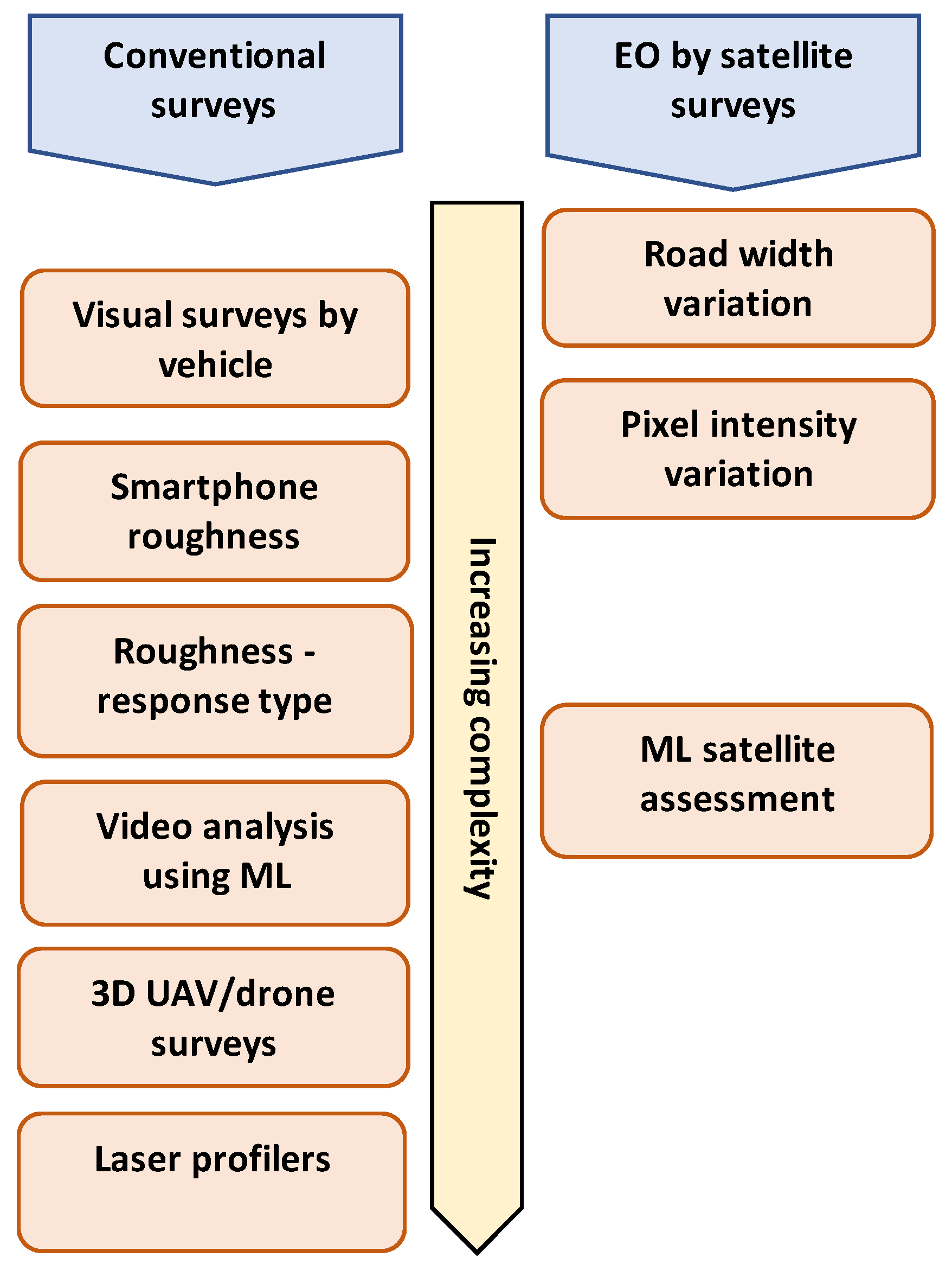
The approach is explained in the context of the objectives of the research, focused on a simple, understandable and sustainable method. Conventional unpaved road condition assessments are conducted using visual inspection from a vehicle. An average condition value is assigned to each road, or section of road, recognising that the condition may vary along that road. As mentioned earlier, conventional surveys are conducted ineffectively, failing to reliably inform maintenance decisions. This methodology addresses these issues and offers a simple, understandable and sustainable solution to the problem that can be applied locally. It is based on the existing regulations and metrics for road condition in Tanzania, to ensure results were useful locally [11]. Figure 1 shows the increasing complexity of the research subjects against conventional condition assessment methods.
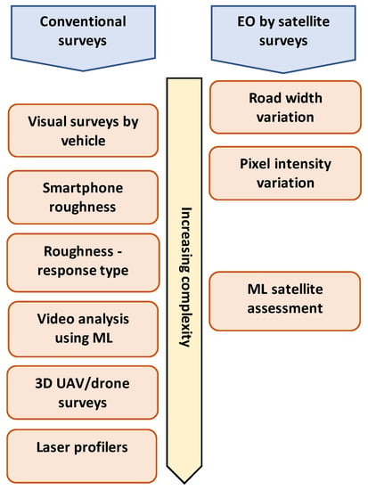
Figure 1.
Diagram to show the increasing complexity of conventional and EO condition assessment methods.
2.1.1. Objective 1
The initial objective of this study was to understand the information required to manage unpaved roads. Therefore, a questionnaire was developed to define aspects of road condition that are crucial for asset management, determine the data requirements to identify these and explore the potential for EO in efficiently collecting these data. The questionnaire results showed that remote sensing was being used by 14% of practitioners on unpaved roads, and by 23% on paved roads. None had used satellites for road condition assessment, but 63% agreed a satellite-derived good/fair/poor condition assessment regime would be useful for unpaved roads. This provided the motivation for proceeding with this research. When asked to propose potential alternative uses for the optical imagery, 73% responded positively with a range of uses including network and maintenance planning, alignment design, maintenance and project monitoring and flood, landslide or disaster monitoring due to climate change. We also explored how practical an EO system would be for LRAs and what appetite there would be for using it. This informed the sustainable approach adopted.
2.1.2. Objective 2
The next objectives were to understand the capability of EO to predict unpaved road conditions, how features can be identified in optical satellite imagery to indicate condition and how this can be managed within a Geographic Information System (GIS) environment. In this work, QGIS software was used as this is freely available and widely used in Africa, which makes it a sustainable tool for use by road authorities in LMICs.
This approach was developed through experience in the original studies [9,10], which were based on subjective assessments and were commensurate with the capacity and resources available in Local Road Authorities in Africa. Engineers who undertook the original studies reported the visible features they used to categorise road condition as the variable road width and variable road surface texture. There was sufficient evidence from those studies to indicate that information contained in the image features could be used to identify condition categories of unpaved roads. The current research focuses on identifying and quantifying that information to measure unpaved road condition.
Width and pixel variation approaches were taken because the results are understandable for engineers with limited knowledge of satellite imagery and would show tangible results to demonstrate their validity.
2.1.3. Objective 3
The third objective was to understand the capability of ML to validate the results from the width and pixel variation study and to provide a more rapid and objective assessment of condition from satellite imagery. This approach is more complex than width and pixel variation and would be more difficult to understand and implement by an LRA. It is, nevertheless, important to consider ML because of the potential time and resource savings that could be achieved. The approach is to identify the condition of specific tiles created from the road surface, and includes establishing a data set, selecting and training ML algorithms to assess the road surface tiles and testing the predictions against the ground truth condition. The research aimed to investigate how ML can help to automate and enhance condition assessment using satellite imagery.
2.1.4. Objective 4
Finally, we have assessed how practical and useful the information or new technology provided by the research would be for asset management of unpaved rural roads. This includes examining how a system could be incorporated into existing maintenance planning and prioritisation systems.
2.2. Imagery and Ground Truthing
The method employed uses high-resolution imagery. The same imagery was used for all three approaches. The LRA in Tanzania provided road conditions. These were checked with the ground truth using visual surveys, smartphone roughness and video analysis.
2.2.1. Satellite Imagery
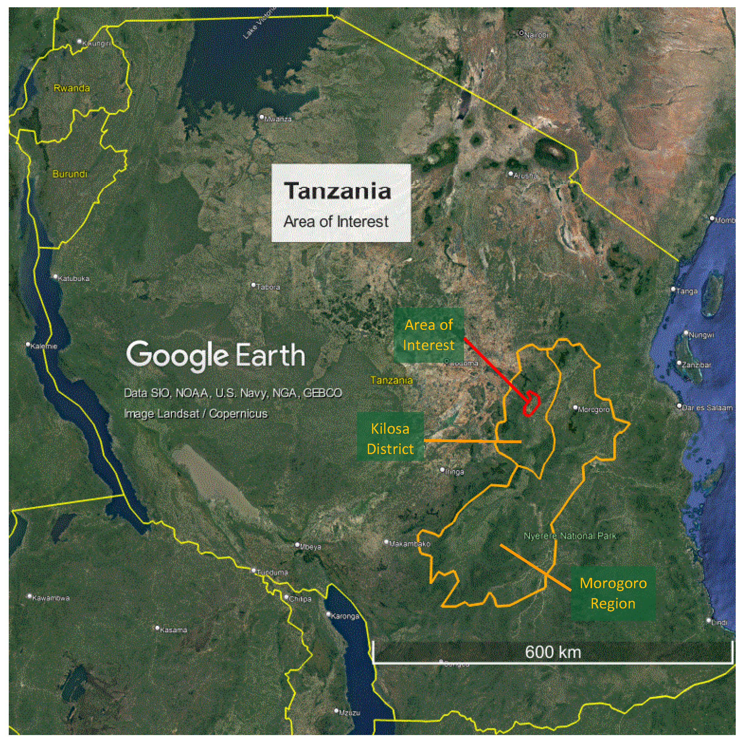
Optical satellite imagery was acquired for a designated area of interest (AoI) within Kilosa district, Morogoro region, Tanzania (Figure 2). The Tanzania Rural and Urban Roads Agency (TARURA) is responsible for these roads and 97.8% of their network was unpaved in 2021 [15]. The AoI encompasses approximately 500 km2 of rural land with two small towns, including 83 local roads with a combined length of 131.7 km. Additionally, the area includes four regional roads with a combined length of 72.3 km, which fall under the jurisdiction of Tanroads, the national roads agency (68.1% of their network remained unpaved in 2021 [15]).

Figure 2.
The area of interest for which the satellite mage was procured.
The imagery to predict the condition of these unpaved roads was obtained from the Pleiades constellation as two ‘geotiff’ images in a panchromatic single band 16-bit format at 0.5 m spatial resolution and in a multispectral four-band 16-bit format at 2.0 m resolution. To enhance the image quality, a pansharpened image was created by fusing both of these images. The fusion process resulted in a high-resolution, natural colour image that was then orthorectified to ensure accurate spatial positioning within a GIS. The final product was a natural colour image with an approximate spatial resolution of 0.5 m.
The image was presented in an 8-bit format, with an intensity range from 0 (black) to 255 (white) for each pixel, depicting the red, green and blue (RGB) spectral bands. This is standard pansharpening processing by the supplier and is a sustainable solution for road engineers in Africa who have limited knowledge of satellite processing. Note that we have previously investigated resolutions of 1.5 m in our initial research in Nigeria using manual assessments [9]. However, the 0.5 m resolution was found to be most appropriate and was therefore applied in this work.
2.2.2. Ground Truthing
The LRA provided condition data for each road in the AoI, which were obtained from a manual condition survey conducted within six months of the date of the satellite image collection. The road conditions were classified into four categories, good, fair, poor or bad, according to the TARURA Defect Identification and Data Collection (DIDC) manual [11]. To validate the condition data reported by the LRA, further ground truth activities were subsequently undertaken by the authors. These were conducted using a drive-through survey, collecting condition information using DIDC visual assessment forms. This was supported by dashcam videos of the road surface and the road roughness measured using a smartphone app called RoadLab Pro, recorded as the International Roughness Index (IRI) in m/km. The dashcam videos proved to be useful later when “revisiting” roads that exhibited variation in condition. Additionally, the smartphone app provided an objective measurement of the roughness of the roads surveyed, and the IRI is directly associated with road condition, according to the standards set in Tanzania [11]. This ground truth was conducted within six weeks of the acquisition of the satellite imagery in February 2018. The findings of the process showed that 87.2% of road condition ratings were consistent with the data provided by the LRA. Further consultation with the LRA was undertaken to clarify the reasons behind any discrepancies. For example, it was revealed that some roads received maintenance between the LRA and ground truth survey, or that the LRA condition survey had actually been conducted earlier in the year, leading to a higher likelihood of change in condition between the surveys. To ensure accuracy of the measurements, the 12.8% of roads where the LRA condition did not agree with the ground truth condition were excluded from the data set. Consequently, a reliable and usable data set comprising 118.76 km of local roads and 59.07 km of regional roads, totalling 177.83 km, was established. This research focused on the local roads maintained by TARURA.
3. Results: Experimental Study
The results are reported for each analysis method used.
3.1. Variation in Width
3.1.1. Variation in Width-Method
Variability in width was identified in previous studies as a feature that could indicate condition using potential physical changes to the road edges and hence width. Engineers reported road width as a feature that helped them to categorise road condition. The assessment process was subjective, so width variability was not quantified. Under this research, experimental trials were conducted to explore the relationship between road width variation and the condition of a road.
Average width data were examined for Kenya and Tanzania, and despite a tenuous relationship between average width and condition, there were too many variables to draw conclusions. This method was therefore excluded as a potential indicator.
Variation in width was then explored. As unpaved roads deteriorate, their width changes due to patterns of use [16,17], as shown in Figure 3 and Figure 4. Variation in width was therefore examined as a potential indicator of condition. It is a simple and tangible concept that engineers with experience of rural roads can understand. This is important to produce a sustainable solution.
Deterioration of unpaved roads is influenced by factors such as climate, traffic, material quality and maintenance. As a road deteriorates, the usable area and hence width of the road undergoes changes. The usable width of a road is defined in this work as the widest area of the road surface over which vehicles can traverse, regardless of the presence of any defects within this area [16]. As unpaved roads lack a restraint system, such as kerbs, their width can vary as a result of overriding [17]. The surface is also vulnerable to water penetration, leading to softening and potential damage caused by vehicles [18]. In summary, our research proposed that variation in road width could be used as an indicator of deterioration resulting from two physical mechanisms:
Widening: The width can increase if damage occurs in the centre of the road that causes drivers to manoeuvre to avoid the damaged areas. The shoulders and side drains are often used, which causes them to become filled with loose material. This effectively extends the usable area of the road and hence the usable width, as shown in Figure 3.

Figure 3.
Usable area of a road surface damaged in the centre.
Figure 3.
Usable area of a road surface damaged in the centre.

Narrowing: Roads can become narrow when the shoulder or road edge is eroded through traffic or rainfall, restricting the usable area. This typically occurs if a side drain becomes blocked or is not working properly. This diverts the flow of water towards the road, softening the surface and causing erosion, as shown in Figure 4.

Figure 4.
Usable area of a road surface damaged at the side.
Figure 4.
Usable area of a road surface damaged at the side.

Methods to measure variation in width were trialled through experimentation, and included standard deviation, variance, nearest neighbour and road width variance. Standard deviation and variance results were inconsistent for different lengths of road and were hence excluded. Nearest neighbour lacked consistency with the ground truth, so was also excluded.
The variation in width was quantified using a formula for road width variance, which was adapted from the road profile variance formula introduced by Jamieson [19].
Road width variance = (moving average of width − width)2
To develop the measurement of road width from satellite images, a representative sample of roads was selected from the AoI that included gravel and earth roads, rural and semi-urban roads and flat or hilly terrain. Road widths were measured using the ‘Measure Line’ tool in QGIS to manually measure the distance between the edges of the road at regular spacings of 5 m (this spacing was determined following experimentation with various spacings). Through experimentation, a moving average window size of nine readings (45 m) was selected to report the road width variation.
3.1.2. Variation in Width-Results
Box and whisker graphs were employed to show how the condition assessment for gravel roads and earth roads relates to road width variations in Figure 5a,b. Whilst both road types show increasing width variance and the ground truth condition worsens from poor to bad, there is significant variability. This poses challenges in setting thresholds to define condition according to width variance.
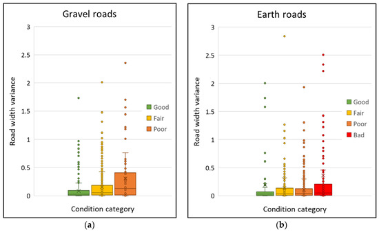
Figure 5.
Box and whisker graph of road width variance for different road conditions: (a) gravel roads and (b) earth roads.
When the gravel road width variance data were plotted in relation to distance (in order of decreasing condition category), it could be seen that the peaks in the variance data increase as the road condition worsens—Figure 6.

Figure 6.
Graph of road width variance against road width for different conditions, gravel roads.
For earth roads, there was a less consistent agreement as the condition worsens (Figure 7). When the earth road data were explored further, some anomalies were detected, which caused anomalous peaks in the variance data on good and fair roads. For example, it was found that the widening of roads in good condition at bends (to facilitate safe passage of longer vehicles) adversely affects the results. Another anomaly involved an artificially fixed boundary on a semi-urban road.

Figure 7.
Graph of road width variance against road width for different conditions, earth roads.
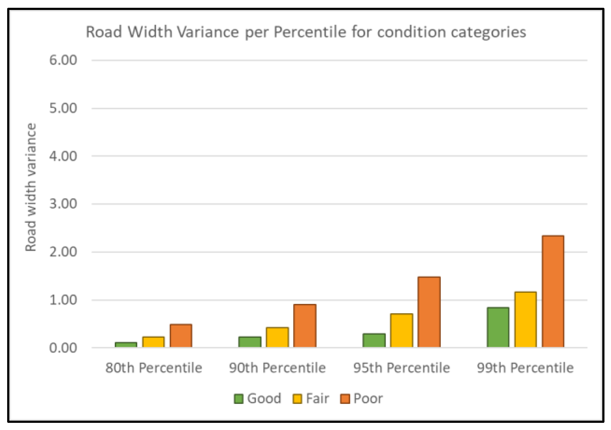
The 80th, 90th, 95th and 99th percentiles were calculated for each condition category, revealing a consistent pattern for gravel roads, as shown in Figure 8. This suggests that a threshold could be set to help differentiate between the different road conditions. For earth roads, a similar behaviour was observed, but only after the removal of the anomalous lengths giving rise to the peaks discussed above—Figure 9. The analysis suggests that measuring variations in road width and setting a threshold such as the 80th percentile could potentially serve as a parameter for detecting lengths in poorer condition.
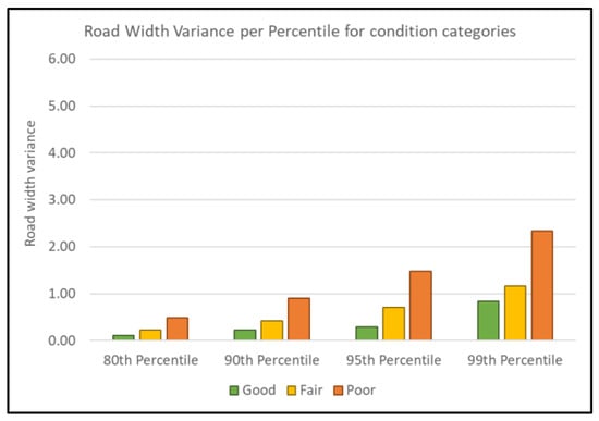
Figure 8.
Road width variance per percentile for each condition category on gravel roads.
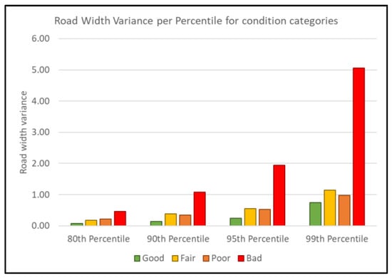
Figure 9.
Road width variance per percentile for each condition category on earth roads after removal of anomalous data.
Due to the number of variables, road width variation would be best suited as a secondary indicator of condition to support pixel variation.
3.2. Variation in Pixel Intensity
3.2.1. Variation in Pixel Intensity-Method
In this study, we sought to develop a more automated approach to condition classification by examining the variation in pixel intensity within images. The idea behind this approach is that images of the surface of unpaved roads in better condition should have a more even colour balance or narrow variation in pixel intensity. Damaged areas on the road surface cause inconsistencies in material properties, shape and moisture content, which create shadows and differences in colour and brightness on a satellite image, and can therefore indicate condition.
Engineers in the original research identified visible changes in road surface texture as an indicator of condition. This was a subjective assessment but showed that the visual characteristics of an unpaved road captured in optical satellite imagery provide valuable information regarding its surface condition [10]. Certain features observed exhibit discernible variations in colour and brightness, which can serve as indicators of condition. The results demonstrated sufficient success at predicting condition to warrant further investigation.
Experimental trials were conducted to explore the relationship between spectral band intensity in the optical image of a road surface and the condition of that road. The distribution of pixel intensity in a histogram shows that a higher variation across the spectral bands indicates a poorer condition surface. This methodology builds on the conventional approach to unpaved road condition assessments, where parameters are derived from surface measurements.
There is no precedent for this on unpaved roads, but Emery [20] found that asphalt road quality is linked to its brightness and heterogeneity using high resolution satellite imagery. Pan [21] also found that asphalt ageing and quality can be determined using spectral mixture analysis from satellite imagery. Pidwerbesky [22] used digital image processing to quantify the relative change in luminance intensity between adjoining pixels in an image of a paved road surface to indicate surface texture. This was tested against the qualitative rating of a human expert. These principles informed the current approach for unpaved road surfaces.
The satellite images in Figure 10 show roads in different conditions, which demonstrates the variation in colour and brightness between the conditions. This information is contained in each pixel and can be accessed in QGIS.

Figure 10.
Road surface variation between different condition categories. Image: © CNES (2017), Distribution AIRBUS DS.
The pixel intensity was measured by selecting samples along each road in order to analyse the distribution of red, green and blue (RGB) pixels. The sum of RGB bands is a measure of colour variation, which as noted above can suggest changes in surface material, shape and moisture, which are indicative of road condition. To ensure that each assessment of variation included an adequate number of pixels while still remaining within the road’s width, a sample area measuring 20 m by 3 m was defined. A total of 6009 samples were available. However, the data sets were imbalanced across the different condition categories. From this pool, a statistically significant population size of 371 samples was randomly selected for analysis using disproportionate stratified random sampling.
In QGIS, each sample was identified by measuring its location using the ‘Measure Line’ tool along the road centre line. The sample was then identified on a separate shapefile layer by drawing a polygon and extracting the polygon as a raster image using the ‘Clip by mask layer’ tool. The maximum and minimum values for each band were visible under ‘symbology’ and a histogram can be created for the data using the ‘compute histogram’ tool. This provided the data for the pixel variation analysis. Note that samples were visually inspected for occlusions and confounding factors and replaced by the next randomly selected sample where necessary.
To assess the performance of the technique, we applied a confusion matrix approach, which compares the ratings reported by the pixel variation and ground truth methods for each length of the test data set. The evaluation of classifier performance is centred on key metrics including recall, precision, F1 and False Positive Rate (FPR). Their functions are:
- Recall: measures the proportion of actual positives identified correctly.
- Precision: measures the proportion of positive identifications that were correct.
- F1: the harmonic mean of recall and precision; a balanced measure of performance.
- FPR: measures the proportion of false positives compared to all positive predictions.
These metrics were chosen to align with the primary objective of the LRA, which is to identify all roads that may require maintenance, particularly those in poor and bad condition. Recall is a key metric because it indicates the success of the model to identify those roads in need of maintenance. F1 is particularly useful in this research due to the imbalanced data set, providing a balanced overview of the results. FPR indicates how many false positives are predicted, which is a priority for the LRA to avoid unnecessary inspection and work on roads that do not immediately require attention.
3.2.2. Variation in Pixel Intensity-Results
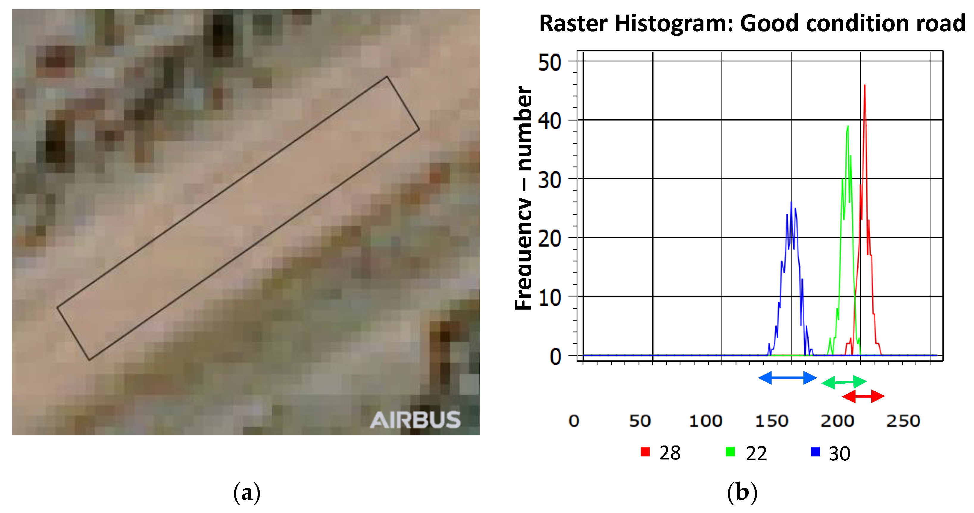
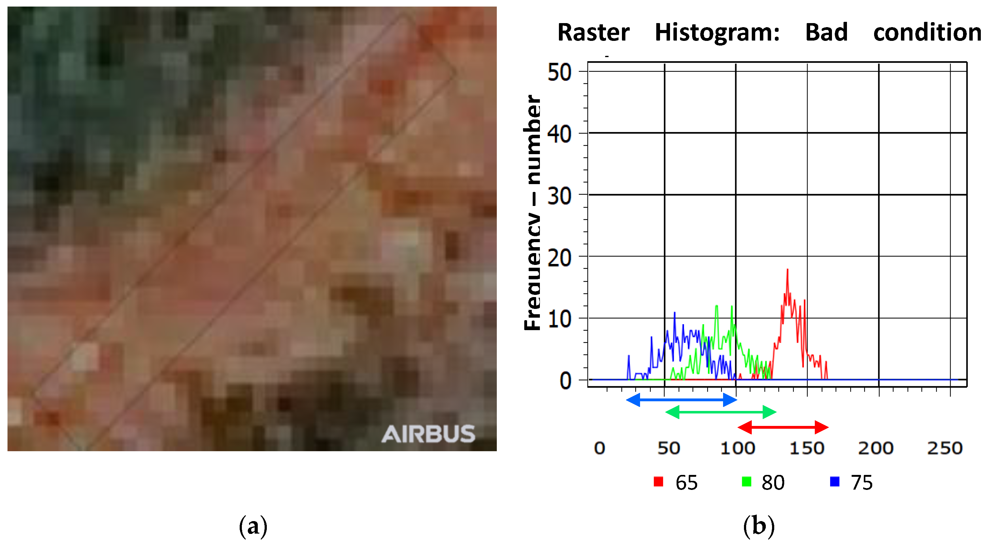
Unpaved roads exhibit a distinct spectral signature when represented on a histogram, as shown in Figure 11a,b and Figure 12a,b. This demonstrates that we can consider the pixel variation range to be in the range of red, green and blue pixel values. For the good condition example, this would be 80 (28 + 22 + 30) (Figure 11b), and for the bad condition road, it would be 220 (65 + 80 + 75) (Figure 12b).

Figure 11.
(a) Satellite image of a road in good condition with sample area indicated by black polygon; (b) histogram of road in a good condition. Image: © CNES (2017), Distribution AIRBUS DS.

Figure 12.
(a) Histogram of a road in bad condition with sample area indicated by black polygon; (b) histogram of a road in bad condition. Image: © CNES (2017), Distribution AIRBUS DS.
To determine whether pixel distributions can be used to indicate condition, the range of RGB intensities was quantified for each sample length of pavement (which had a corresponding ground truth condition rating) and analysed using a confusion matrix approach to determine the success to which the condition rating resulting from pixel variation agrees with the ground truth rating, as discussed above. To achieve this, it was necessary to allocate a pixel variation condition rating to each length. Through examination of part of the data set (used as a ‘development set’), thresholds were established for the pixel variation ranges for each condition category. Whilst our initial work considered gravel and earth roads separately, we noted that previous consultations had found that most countries consider earth and gravel roads similarly when assessing their condition. In addition, we found that the thresholds identified for earth and gravel roads were very similar. Therefore, we decided to combine the two data sets using a single set of thresholds shown in Table 1. The results from individual spectral bands showed no advantage over a combined value when tested experimentally using the pixel variation method. Note that, in practice, the thresholds would be adjusted to the particular needs of the LRA.

Table 1.
Combined thresholds for the combined gravel and earth data set.
The performance in the classification of condition when applying the combined thresholds is shown in Table 2. Table 2a is the sample population and Table 2b shows the analysis results for the selected metrics. Individual results are particularly high for recall on good condition roads.

Table 2.
Results for combined local road development data set: (a) population and (b) assessment metrics results.
When the results were aggregated, it became evident that the prediction accuracy for gravel roads surpasses that of earth roads across all metrics, as shown in Table 3. For the development data set, the crucial metric of recall is 23.3% more accurate, although the gravel FPR result is 0.1% less effective compared to earth roads.

Table 3.
Local road development results for gravel, earth and combined data sets.
Note that the above results include the lengths that were used to develop the thresholds, potentially producing some “bias” in the outcomes. Therefore, we withheld some data for use only in testing of the performance. When these lengths were assessed, the combined data set returned an overall accuracy of 71.9%, compared to the 77.7% in the development set in Table 3. The precision was also lower at 17.6% for roads in bad condition, but this can be attributed to the low population of samples for the bad category in this set, totalling six.
A summary of the individual results for each condition category, for both the development and testing data sets, can be seen in Table 4. This shows results for the combined gravel and earth road data sets, disaggregating based on different road conditions. When analysing roads in bad condition, which is of particular importance for LRAs, high levels of accuracy were achieved in both the development and testing stages. However, it should be noted that the performance of other metrics was less satisfactory in comparison.

Table 4.
Disaggregated results for the combined data set for all conditions.
3.3. Machine Learning
3.3.1. Machine Learning-Method
ML was explored as a method to validate the results from the width and pixel variation study. It has the potential to provide a more rapid and objective assessment of condition from satellite imagery. Although this approach is more complex and would be harder to understand by an LRA, it has significant potential to save time and resources. ML has been used to assess condition of roads using EO satellite and UAV imagery [12,13,14], but the shortcomings were highlighted above. These studies focused on paved roads, but are useful to inform how a system could be developed for unpaved roads.
The ML approach for measuring condition using satellite images was used as a way to objectively justify the use of pixel variation as a method to measure condition. It is also a test of the feasibility for developing a framework for assessing unpaved road conditions rapidly and consistently in the future. Other advantages of using this process would be that large areas can be assessed at the same time and the process can be checked to ensure the results are robust.
A systematic procedure was developed to automatically identify and create road image samples for processing using ML. A vector layer was created with samples of approximately 3 m by 3 m. Using the QGIS ‘Clip by Mask layer’ tool, the tiles were split and created as separate raster images, with each tile being labelled as good, fair, poor or bad. These samples were then analysed using ML algorithms.
Note that classical ML algorithms tend to work more effectively with square images [23]. Although modern algorithms can accommodate any shape, it is common to use square inputs for designing models to avoid processing issues. Samples for this research were formed in squares of between 6 and 8 pixels so they would fit within the surface area of the road. The sample size differed from that used for the manual pixel variation method above, but they were created from the same data set. During a visual examination of the pixel samples, it became evident that data cleaning procedures would be necessary to ensure quality of the samples. Samples that displayed occlusions or irregular shapes, particularly those located at the end of a road, were removed.
The image data were divided into training/validation and testing subsets, with an approximate ratio of 80:20. The training set was used to train the ML classifier, which was then tested using the test set to assess the agreement between ML-derived condition categories and the ground truth category, with the accuracy defined as the number of correct predictions divided by the total number of predictions.
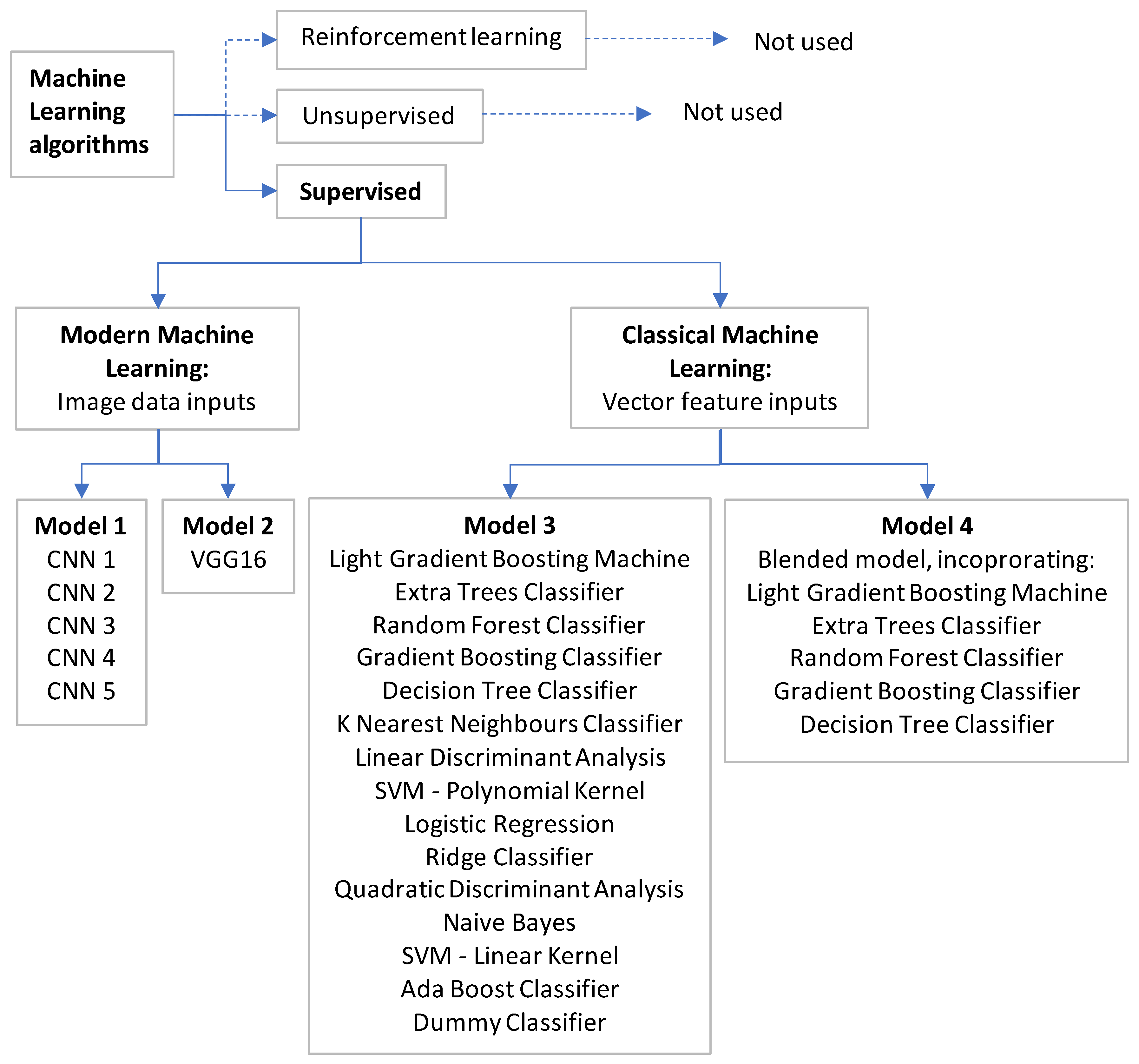
Four different ML techniques were tested as shown in Figure 13: customised Convolutional Neural Networks (CNNs), transfer learning using VGG16, classical ML algorithms and a blended model from the classical algorithms.
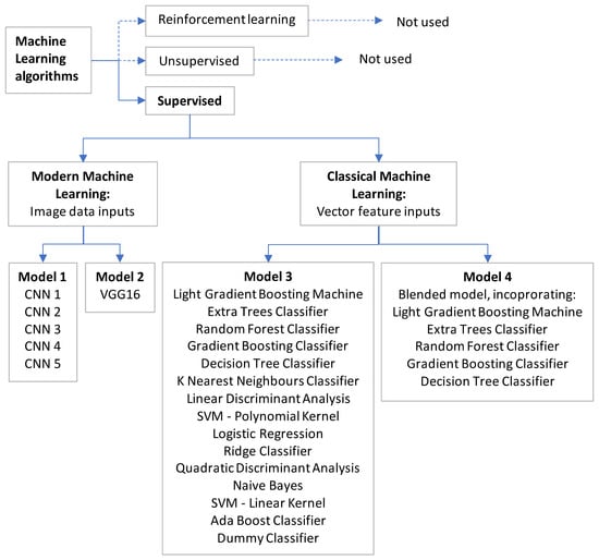
Figure 13.
Machine Learning models used in the research.
Five customized CNNs (Model 1) were engineered and labelled as CNN1 through CNN5. CNN1 and CNN2 comprise two repeated stacks of convolutional layers (CL), a Rectified Linear Unit (ReLU) and a dropout layer (DL), followed by four and five fully connected layers (FC), respectively. CNN3 shares a similar architecture to CNN2 but uses fewer filters in the fully connected layers. CNN4 introduces more variety in the fully connected layers by employing different filter settings and dropout rates yet maintains the same overall structure as the previous models. Finally, CNN5 simplifies the configuration with only two stacks of convolutional layers, ReLU, max-pooling and dropout, followed by two fully connected layers, providing more streamlined architectural variants in comparison to the more complex configurations of CNN1 to CNN4.
These CNNs can import images and assign importance to various aspects in the image, differentiating one from the other. The CNN works by using filters to capture spatial and temporal dependencies in an image, reducing the image into a form that is easier to process without losing those features that are critical for a good prediction. It generally requires less pre-processing than other classification algorithms [24].
A transfer learning approach using a pre-trained network VGG16 (Model 2) was evaluated because it has demonstrated success in image classification [25], despite being originally designed to extract features from objects. However, the VGG16 model requires a minimum image size of 64 × 64 pixels, leading to resizing of the samples using an interpolation algorithm, which produced imprecise images.
For the classical ML algorithms (Model 3), a total of 15 supervised ML algorithms were used for classification, as shown in Figure 12. Processing was carried out in both red–green–blue (RGB) and Hue–Saturation–Value (HSV) spaces, along with texture features of energy, homogeneity, contrast, correlation, dissimilarity and angular second moment. Eigenvectors were extracted for both colour and texture for each sample.
In Model 4, the blended model was engineered, integrating the top five high-performing individual classifiers from Model 3 to generate a more precise final prediction. This approach leverages the combined predictive strengths and mitigates the potential weaknesses of each model, thereby refining the overall prediction quality.
3.3.2. Machine Learning-Results
Model 1: CNNs. Among the five CNNs, CNN2 yielded test results with the highest overall accuracy of 81%, but with a recall of 61% and F1 of 76%. CNN1, 3 and 5 performed the best in recall in the bad condition, with results of 91%, 85% and 91%, respectively, which is a priority for LRAs. F1 was also high for the same categories at 95%, 92% and 93%. These outcomes indicate a satisfactory level of accuracy in predicting roads in bad condition, making the CNN a viable candidate for further research.
Model 2: VGG16. A transfer learning approach using the pre-trained VGG16 network exhibited an overall test accuracy of 63%, with F1 results ranging from 51% and 71%. It is noted that the primary purpose of the VGG16 algorithm is to identify features in an image, whereas the focus of this research is to classify condition. Additionally, the accuracy of the algorithm may have been adversely affected by the resampling process. The application of VGG16 to this problem did not yield satisfactory outcomes and would necessitate further refinement to enhance its performance.
Model 3: Fifteen Classical ML classifiers. Road surface condition eigenvectors were determined to construct a database of characteristics, which were then used to train the ML classifiers to categorize the road surface conditions. Key colour and texture features used included mean, variance, skewness, energy, contrast, correlation and dissimilarity.
The performance of all classifiers varied, with the top five performing being Light Gradient Boosting Machine, Extra Trees Classifier, Random Forest Classifier, Gradient Boosting Classifier and Decision Tree Classifier, with accuracies ranging from 86.7% to 81.3%. These five were all taken forward to comprise the blended model shown in Model 4.
Model 4: Blended model. From the 15 classical ML classifiers, the top five were used to produce a blended model. Blending was achieved by using a hard voting system, which is considered as the most appropriate for a classification task [26]. The results from this model demonstrate an overall accuracy of 94% for the test set, with a recall for roads in bad condition of 96% and demonstrating high scores across all metrics, as shown in Table 5.

Table 5.
Confusion matrix showing the results of the classical ML classifier test model.
The ML trials demonstrated a high overall accuracy, reaching up to 94%. These findings were supported by favourable recall and FPR results. Classical ML algorithms proved to be the most successful, although CNNs also performed well.
4. Discussion
To overcome the challenges associated with the measurement of condition of roads in LMICs, in this work, we have proposed three potential methods that could be applied to satellite images to report condition within four categories. Our first method, road width variation, is manual but simple to understand. However, whilst it gives a broad assessment of condition, there is a high level of variability in the allocation of categories. The requirement for manual assessment makes the method less practical, but the development of an automated system would need to overcome many challenges before a reliable system could be feasible.
The variation in pixel intensity process demonstrates higher accuracy than the width variation and is more automated. To assess the applicability of the results to an LRA, key metrics such as recall, F1 and FPR were employed. By applying predefined thresholds, the findings indicate that overall accuracies ranging from 70% to 80% can be expected, with recall rates reaching up to 87% and minimal false positive predictions. This suggests that LRAs have the opportunity to adjust thresholds to prioritise specific parameters with higher accuracy, thereby increasing confidence in the assessment.
The ML trials demonstrated the highest accuracy, with favourable results for key metrics. Overall accuracies of up to 94% were achieved. The classical ML blended model and the CNNs performed satisfactorily in terms of overall accuracy, as well as in the key metric of recall. Both show potential to be used as ML models for the assessment of unpaved road condition using satellite imagery.
Given the practicality and performance of the ML approach, we propose that a framework could be applied to classify unpaved road condition utilising the classical ML blended model. This framework is shown in Figure 14. The first step is to define the needs of the LRA, which includes reviewing the current knowledge of unpaved roads and establishing road locations so far as is possible. This should identify any necessary institutional reform and capacity building to support the sustainability of the framework.
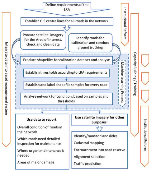
Figure 14.
Framework for unpaved road condition classification using satellite imagery and machine learning.
In order to adapt the model to a specific country or region, a calibration process will be necessary, which can be conducted by using representative roads to compare actual conditions to ground truth conditions and setting parameters for each condition category. This process ensures that the model is trained and adjusted according to local conditions. Additionally, the LRA will need to determine appropriate thresholds that align with their specific requirements. Some necessary activities can be developed as GIS plug-ins, such as labelling the samples. An ML model would then be established to categorise the roads into overall condition categories, producing a high-level overview of unpaved network conditions.
Asset management of rural road networks in Africa suffers from a lack of information on unpaved roads, and maintenance is reliant on unstructured data collection and ad hoc reporting of conditions [27]. Application of this framework would introduce a structure to the process of planning and prioritising maintenance by proposing regular and objective assessments of the condition of roads, whilst building a robust record of condition data, where roads are deteriorating and at what rate. The traditional maintenance procedure is to find faults and fix them with the available budget. This framework would provide the opportunity to help set service levels and deliver maintained roads for the lowest cost. The solution is scalable to a country level, and large volume acquisition of satellite imagery offers opportunities to reduce costs by procuring on a large scale. However, there are some potential challenges that remain to be overcome, as discussed in the following section.
Remaining Challenges
Although progress has been made in the development of methods to improve the ability to assess road surface condition using satellite imagery, challenges remain:
Road classes: This research primarily targeted local roads, which in Tanzania are most important in addressing rural poverty, yet often receive minimal maintenance. These roads have also been relatively under-studied, resulting in a lack of information on inventory and condition, making this technology particularly beneficial for the local road network. While regional roads were also considered, their inclusion may present some challenges due to the involvement of two different road authorities.
Data sets: Upon establishing and categorising the road conditions, it became apparent that the total lengths differed amongst each category, resulting in an imbalanced data set. Specifically, there were small sample populations for poor gravel roads (80 samples) and good earth roads (29 samples), and no gravel roads were found in bad condition. To address this imbalance and to ensure proper representation of all categories, a disproportional stratified random sampling approach was used. It is recognised, however, that some metrics such as overall accuracy do not perform well on imbalanced data sets.
Occlusions: Some roads in the study area exhibited occlusions that hindered the visibility of the road edge and/or surface. In cases where the presence of occlusions was excessive, making an accurate measurement of road width impossible or significantly obscuring the road surface, the road was excluded from the trial. It should be noted that even small objects can have an impact on the pixel variation, making data cleaning important. However, certain occlusions possess distinctive spectral signatures that could potentially be automatically identified. Further research would be required to explore and develop the potential to automatically identify occlusions.
Road geometry: Road design may include certain features that artificially constrain the road geometry and limit the potential variation in usable width due to condition. These features can include splay at junctions, curve widening, structures and terrain where roads are excavated into a hillside. The presence of these features can impose constraints on the road width and potentially introduce confounding factors that affect the results.
5. Conclusions
The implementation of an automated EO system for identifying unpaved road conditions offers numerous advantages. Firstly, it enables an impartial, consistent and regular assessment of the road network, facilitating informed decision making in prioritising road maintenance activities. Secondly, it mitigates the logistical challenges and associated risks inherent in traditional condition assessment systems. Additionally, it is environmentally efficient, aligning with climate mitigation goals by reducing the need for on-site inspections and minimising carbon emissions. Integrating this system with a Road Asset Management System (RAMS) would streamline operations and offer a potentially cost-effective solution for generating high-level data to support road maintenance prioritisation. It would also allow change detection at a scale that is not currently possible using current methods and techniques. These benefits collectively enhance the efficiency and effectiveness of LRAs in managing their rural road networks.
We have proposed a framework in which this approach could be applied. This framework offers flexibility to accommodate various strategies and data requirements, enabling LRAs to customise the information they receive based on their specific priorities. This would enable LRAs to rapidly identify roads needing further inspection and prioritise urgent maintenance interventions. The framework provides a rapid, objective and consistent approach that has the potential to be cost effective. Furthermore, it can be integrated with modern GIS-based asset management systems and addresses current challenges faced by LRAs in road condition assessment and management.
Author Contributions
Conceptualisation, R.W. and Z.W.; methodology, R.W.; software, Z.W.; validation, P.W. and A.W; formal analysis, R.W. and Z.W.; investigation, R.W. and Z.W.; resources, R.W.; data curation, R.W.; writing—original draft preparation, R.W.; writing—review and editing, R.W. and P.W. and A.W.; visualisation, R.W.; supervision, P.W. and A.W.; project administration, R.W.; funding acquisition, R.W. All authors have read and agreed to the published version of the manuscript.
Funding
This research received no external funding.
Data Availability Statement
The satellite imagery used in this research is controlled by license restrictions and cannot be made available publicly. Some data presented in this study are available on request from the corresponding author. The data are not publicly available as permission will need to be sought from the Local Road Authority in the study country.
Acknowledgments
I would like to thank Chris Kettell and Alix Edwards of TRL for their support in technically reviewing this document, and Kamal Nesnas of TRL for his advice on use of machine learning models.
Conflicts of Interest
The authors declare no conflict of interest.
References
- Ngezahayo, E.; Burrow, M.; Ghataora, G. Rural Roads–roles, challenges and solutions for Sub-Saharan Africa’s sustainable development. Int. J. Latest Eng. Manag. Res. 2019, 4, 70–79. [Google Scholar]
- Pinard, M.; Mbvundula, W.D. Strategy for Improved Road Asset Management in Southern Africa. In Proceedings of the Sixth International Conference on Low-Volume Roads, Minneapolis, MN, USA, 25–29 June 1995. [Google Scholar]
- Harral, C.G.; Faiz, A. Road Deterioration in Developing Countries: Causes and Remedies; The World Bank: Washington, DC, USA, 1988. [Google Scholar]
- Hine, J.; Sasidharan, M.; Eskandari, T.M.; Burrow, M.P.N.; Usman, K. Evidence on Impact of Rural Roads on Poverty and Economic Development; K4D Helpdesk Report; Institute of Development Studies: Brighton, UK, 2019. [Google Scholar]
- AfDB. Tracking Africa’s Progress in Figures, Chapter 5: Infrastructure Development; African Development Bank Group: Tunis, Tunisia, 2014; Chapter 5; p. 51. [Google Scholar]
- Paige-Green, P.; Verhaeghe, B.; Head, M. Climate Adaptation: Risk Management and Resilience Optimisation for Vulnerable Road Access in Africa, Engineering Adaptation Guidelines; GEN2014C; ReCAP for DFID: London, UK, 2019. [Google Scholar]
- Sustainable Mobility for All. Global Roadmap of Action toward Sustainable Mobility: Universal Rural Access; Creative Commons Attribution: Washington, DC, USA, 2019. [Google Scholar]
- Sayers, M.W.; Gillespie, T.D.; Queiroz, C.A.V. The International Road Roughness Experiment Establishing Correlation and a Calibration Standard for Measurements; World Bank Technical Paper No. 45; The World Bank: Washington, DC, USA, 1986. [Google Scholar]
- TRL. Case Study: Transport Infrastructure Monitoring Project; Satellite Applications Catapult, Innovate UK: Oxford, UK, 2015. [Google Scholar]
- TRL. The Use of Appropriate High-Tech Solutions for Road Network and Condition Analysis, with a Focus on Satellite Imagery; Final Report: 2018; ReCAP for DFID: London, UK, 2018. [Google Scholar]
- PO-RALG. Defect Identification and Data Collection Manual: Local Government Road Inventory and Condition Survey Project; PO-RALG: Dar es Salaam, Tanzania, 2005. [Google Scholar]
- Cadamuro, G.; Muhebwa, A.; Taneja, J. Assigning a Grade: Accurate Measurement of Road Quality Using Satellite Imagery. arXiv 2018, arXiv:1812.01699. [Google Scholar]
- Brewer, E.; Lin, J.; Kemper, P.; Hennin, J.; Runfola, D. Predicting road quality using high resolution satellite imagery: A transfer learning approach. PLoS ONE 2021, 16, e0253370. [Google Scholar] [CrossRef] [PubMed]
- Goulding, J. Machine Learning for Road Condition Analysis Part 1: Partnerships. 2018. Available online: https://medium.com/frontier-technology-livestreaming/machine-learning-for-road-condition-analysis-part-1-partnerships-f625caf970a9 (accessed on 16 February 2020).
- Roads Fund Board Tanzania. Annual Report for the Year Ended 30th June, 2021; Ministry of Works: Dodoma, Tanzania, 2022.
- Geddes, R.; Mbabazi, E.; Amara, T.; Chilonda, P. Economic Growth through Effective Rural Road Asset Management; ReCAP for DFID: London, UK, 2019. [Google Scholar]
- Tanzania MoW. Road Geometric Design Manual: 2011 Edition; Ministry of Works: Dar es Salaam, Tanzania, 2012.
- Paige-Green, P.; Verhaeghe, B. Making Africa’s Roads More Resilient to Climate Change; ReCAP for DFID: London, UK, 2018. [Google Scholar]
- Jamieson, N.J. Using Road Profile Variance to Identify Sites That Promote Poor Ride Quality; NZ Transport Agency Research Report 352; NZ Transport Agency: Wellington, New Zealand, 2008; 64p, ISBN 0-478-33407-4. ISSN 1177-0600.
- Emery, W.; Singh, C. Large-Area Road-Surface Quality and Land-Cover Classification Using Very-High Spatial Resolution Aerial and Satellite Data, 2014, Remote Sensing of Roads and Highways in Colorado: Quarterly Progress Report #7. Available online: https://trid.trb.org/view/1264145 (accessed on 2 August 2023).
- Pan, Y.; Zhang, X.; Jin, X.; Yu, H.; Rao, J.; Tian, S.; Luo, L.; Li, C. Road pavement condition mapping and assessment using remote sensing data based on MESMA. In IOP Conference Series: Earth and Environmental Science; IOP Publishing: Bristol, UK, 2016; Volume 34, p. 012023. [Google Scholar] [CrossRef]
- Pidwerbesky, B.; Waters, J.; Gransberg, D.; Stemprok, R. Road Surface Texture Measurement Using Digital Image Processing and Information Theory; Land Transport New Zealand Research Report 290; Land Transport New Zealand: Wellington, New Zealand, 2006; 65p, ISBN 0-478-28701-X. ISSN 1177-0600.
- Ghosh, S.; Das, N.; Nasipuri, M. Reshaping inputs for convolutional neural network: Some common and uncommon methods. Pattern Recognit. 2019, 93, 79–94. [Google Scholar] [CrossRef]
- Saha, S. A Comprehensive Guide to Convolutional Neural Networks—The ELI5 Way, towards Data Science. 2018. Available online: https://towardsdatascience.com/a-comprehensive-guide-to-convolutional-neural-networks-the-eli5-way-3bd2b1164a53 (accessed on 24 June 2023).
- Simonyan, K.; Zisserman, A. Very Deep Convolutional Networks for Large-Scale Image Recognition. arXiv 2015, arXiv:1409.1556. [Google Scholar]
- Mohammed, A.; Kora, R. A comprehensive review on ensemble deep learning: Opportunities and challenges. J. King Saud Univ.-Comput. Inf. Sci. 2023, 35, 757–774. [Google Scholar] [CrossRef]
- Saeed, N.; Dougherty, M.; Nyberg, R.G.; Rebreyend, P.; Jomaa, D. A Review of Intelligent Methods for Unpaved Roads Condition Assessment. In Proceedings of the 2020 15th IEEE Conference on Industrial Electronics and Applications (ICIEA), Kristiansand, Norway, 9–13 November 2020; pp. 79–84. [Google Scholar] [CrossRef]
Disclaimer/Publisher’s Note: The statements, opinions and data contained in all publications are solely those of the individual author(s) and contributor(s) and not of MDPI and/or the editor(s). MDPI and/or the editor(s) disclaim responsibility for any injury to people or property resulting from any ideas, methods, instructions or products referred to in the content. |
© 2023 by the authors. Licensee MDPI, Basel, Switzerland. This article is an open access article distributed under the terms and conditions of the Creative Commons Attribution (CC BY) license (https://creativecommons.org/licenses/by/4.0/).

