Abstract
Reasonable allocation of space-based radar resources is a crucial aspect of improving the accuracy of space multi-target tracking and enhancing spatial awareness. The conventional resource allocation algorithm fails to exploit the high dynamic radar cross-section (RCS) characteristics, resulting in poor tracking robustness, tracking divergence, or even loss of tracking. However, the RCS of space targets fluctuates considerably in actual tracking scenarios, which cannot be disregarded for space target tracking tasks. To address this issue, we propose an adaptive allocation method that considers the dynamic RCS fluctuation characteristic for space-based radar tracking assignments. The proposed method exploits the predictable orbital information of space target to calculate the real-time observation angle of radar, and then obtains the multi-target dynamic RCS through the target RCS dataset. By combining the obtained RCS sequence, radar power, and bandwidth, an optimal model for radar tracking accuracy is established based on the multi-target posterior Cramér–Rao lower bound (PCRLB) to evaluate the tracking performance. By resolving the aforementioned multivariance optimization problem, we eventually acquire the results of power and bandwidth pre-allocation for tracking multiple space targets. Simulation results validate that, compared with the traditional methods, the proposed joint dynamic RCS power and bandwidth allocation (JRPBA) method can achieve superior tracking accuracy and minimize instances of missed tracking.
1. Introduction
1.1. Background and Problem Statement
With the growing exploration of space activities, effective tracking, monitoring, and protection technology for various space targets has brought significant attention to the field of space situational awareness (SSA) region. In [1,2,3], an analysis is conducted on the number of space targets launched by the United States, Europe, the Soviet Union, and China in recent years, as well as the evolving trend of additional space debris generated.
Therefore, sparing no efforts on space resource development, space security and space control [4,5] is indeed necessary for enhancing the SSA ability of a nation. Many countries and regions have developed ground-based equipment for the SSA task. For instance, the European Incoherent Scatter Scientific Association (EISCAT) has developed three incoherent scatter radar systems, and the operating frequency of the two radars located in northern Scandinavia are 224 MHz and 931 MHz, while the other one in Svalbard operates at 500 MHz. The operating frequency of the Italian Bi-static Radar for LEO Tracking (BIRALET) system ranges from 410 to 415 MHz [6]. The Tracking and Imaging Radar (TIRA) in Germany is a system devoted to detailed studies of satellites and space debris, and contributes to European SSA [7]. The United States Space Surveillance Network (SSN), operated by the United States Strategic Command (USSTRATCOM), consists of a worldwide network of 29 space surveillance radars and optical telescopes [8]. The French air force has operated the GRAVES bistatic radar system since 2005 [9].
However, it should be noted that the space-based radar system is superior to both ground-based equipment and space-based optical systems. Unlike other systems, it can monitor space targets of interest in all weather conditions, regardless of the Earth’s curvature or weather constraints. Therefore, we focus on implementing a space-based radar system to track multiple space targets in this paper. It is worth emphasizing that enhancing the accuracy and efficiency of multi-target tracking using space-based radar has been a significant research topic in recent years.
Space-based radars can accomplish simultaneous multi-beam tracking of space targets by carrying a collocated multiple input multiple output (C-MIMO) radar payload. As a new system radar, C-MIMO radar launches different beams to multiple targets by means of transmitting waveform diversity, which can accomplish simultaneous multi-beam tracking of space targets [10,11,12,13,14]. The technology addresses the limitations of traditional phased array radar (PAR) time-sharing tracking and is extensively applied in multi-target detection and tracking. Nevertheless, due to the reliance on solar panels for energy supply and hardware design constraints, the power and bandwidth of space-based radar are more restricted compared to their ground-based counterparts. Space targets can achieve relative velocities ranging from several to tens of Mach, causing rapid changes in the azimuth and elevation angles observed by space-based radar. Moreover, the structures of space targets are complex and different. During the tracking process of space-based radar, the radar cross section (RCS) of the space targets exhibits high dynamic variation characteristics. These factors will result in unstable tracking performance of space-based radar. The above-mentioned problems in the field of space-based C-MIMO radar resource allocation research to allocate the limited total transmit power and bandwidth to each transmit beam reasonably are in urgent need of solving, so as to obtain higher space target tracking accuracy.
At present, most research mainly focuses on the tracking resource scheduling of ground-based radar to airmobile targets. Ref. [15] carried out research on the selection and optimization of MIMO radar parameters for multi-target detection and tracking. Ref. [16], the target detection and tracking under the framework of cognitive radar was studied. Refs. [17,18,19] established a cost function based on Bayesian Cramér–Rao lower bound, and used the gradient projection algorithm to obtain the optimal power scheduling results of a radar system for multi-target tracking under different motion parameters. A joint strategy of power and bandwidth scheduling for maneuvering multi-target tracking (MMTT) was proposed in [20] and utilized a relaxation method to obtain the optimized allocation scheme by solving the nonconvex optimization problem. Refs. [21,22,23] studied the resource allocation method for air target tracking for the two institutional configurations of distributed MIMO radar and collocated MIMO radar. Based on the sum of PCRLB of multiple batches of targets, the adaptive allocation scheme of radar resource was realized. Refs. [24,25,26] studied the differentiated tracking resource scheduling scheme, considering the system constraints and external factors comprehensively, they proposed the joint beam and power scheduling (JBPS) method, and realized the global objective function design and solution. The authors of [27] studied the antenna selection or power allocation problem. Most of the existing algorithms are aimed at radar resource scheduling for tracking air target tasks, while the stable space targets have obvious semi-cooperative characteristics which can be further exploited [28]. For instance, the orbit of the space target can be predicted relatively accurately, and its orientation mode is often fixed. So, it is necessary to study the resource scheduling scheme which is more suitable for space multi-target tracking.
In addition, Ref. [29] studied the power allocation scheme of C-MIMO radar for RCS non-fluctuation models and RCS fluctuated models, and verified the effectiveness of the adaptive power optimal allocation algorithm. Similarly, Ref. [30] aims at the problem of C-MIMO radar resource scheduling, the influence factors of distance, RCS, and motion model error are studied, respectively, and the decision-making effect of each factor on radar resource allocation is discussed comprehensively. Ref. [31] studied the low-Earth-orbit (LEO) satellite detection techniques and analyzed the detection capability of various walker constellation space-based radar deployment schemes for space targets. However, the above works only discuss the detection ability of space-based radar with different walker constellations and ignore the target RCS fluctuation characteristic in the radar resource scheduling tasks. The existing works and algorithms simply construct the target RCS as the non-fluctuation model or give RCS simple time-varying characteristic and these assumptions are inaccurate in actual scenarios, which fail to be eligible for the actual high dynamic RCS space target tracking requirements.
1.2. Problem Analysis and Contributions
The existing works have provided a rich theoretical and technical basis for the ground-based radar resource scheduling problem and improved its comprehensive application efficiency. However, this research rarely considers the radar resource allocation problem of space-based radar tracking multiple space targets and does not comprehensively consider factors such as the orbital motion characteristics or dynamic RCS characteristic of space targets.
Bayesian theory points out that prior information can improve the accuracy of parameter estimation. Inspired by this, we can model the on-orbit space target and obtain its full-angle static RCS database and orbit information, which can be introduced into the resource allocation framework as a priori information to solve the above problems. In this paper, we propose an adaptive joint dynamic RCS power and bandwidth allocation (JRPBA) method for multiple space target tracking via space-based radar. The main contributions of the paper are given as follows.
- (1)
- The space satellite target is different from the aircraft target in the air. It mainly moves around the Earth due to the gravity of the Earth. Considering that the space target orientation model is usually fixed, this means that the motion attitude of the space target can be calculated more accurately. Can this semi-cooperative characteristic of space targets be utilized in space-based radar resource allocation to improve tracking accuracy? For space surveillance systems, the space target information database is often continuously constructed and expanded. In this paper, we introduce the space target information database as a priori information into the resource allocation framework. The purpose is to utilize the target information to adopt appropriate signal processing methods for different satellites and take various characteristics of space targets into account in the actual target tracking process to obtain higher multi-target tracking accuracy.
- (2)
- In the actual radar tracking scene, the radar line of sight (RLOS) has a great influence on the target RCS characteristics. Specifically, the RCS sequence of the target shows high dynamic fluctuation characteristics. However, the existing radar resource allocation method does not take into account the dynamic RCS characteristics of the targets, which leads to the fact that the previous radar resource allocation scheme cannot be fully adapted to the actual tracking scene and eventually leads to tracking divergence or even mistracking. In this paper, an adaptive joint dynamic RCS power and bandwidth allocation (JRPBA) method for space-based C-MIMO radar is proposed. The core idea is to reasonably allocate the limited power and bandwidth resources of C-MIMO radar in multi-target high dynamic RCS tracking scenarios by utilizing the semi-cooperative characteristic of space targets and the predictable characteristics of orbit. The mismatched problem between the radar resource allocation scheme and the actual tracking scene is solved and the multi-target tracking accuracy and efficiency of the space-based radar system are improved.
The rest of this paper is organized as follows. Section 2 presents a space target motion model and space-based radar observation model. Section 3 derives the multi-target tracking PCRLB. Furthermore, the dynamic RCS sequence mapping method and the adaptive joint dynamic RCS power and bandwidth allocation method is given in Section 4. Simulation results and conclusions are given in Section 5 and Section 6, respectively.
2. Space Target Observation System Model
2.1. Space Target Motion Model
The schematic diagram of space-based radar observation for space targets tracking is depicted in Figure 1. Note that we assume that space-based radar is able to track space targets in the observation region continuously.
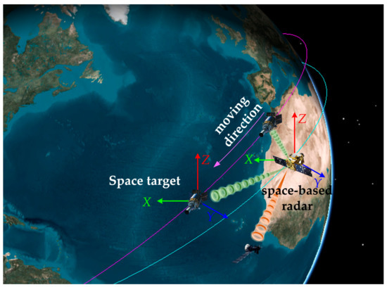
Figure 1.
Schematic diagram of space-based radar observation for space targets tracking.
For the sake of simplicity, assuming that there are Q distinguishable space targets in the three-dimensional observation scene and the targets kinemics motion obeys the constant velocity (CV) mode, the motion model of the q-th target at the k-th sample interval is defined as follows:
where denotes the target state. and represent the range and velocity of the q-th target at the k-th sample interval in the Cartesian coordinate system. represents the state transition matrix of q-th target.
where and represent the Kronecker operator and sample interval of adjacent tracking moments, respectively. The matrix denotes the 3 × 3 identity matrix. In the above motion model, the matrix is modeled as a multidimensional Gaussian distribution with zero-mean and the covariance , which is used to represent the random error or fluctuation of the target motion state. Its covariance is expressed as [32]:
where is the process noise coefficient that has the ability to adjust the size of .
2.2. Space-Based Observation Model
Assume that the C-MIMO radar with coordinates of tracks multiple space targets with the simultaneous multi-beam mode. After all the radar echo signals are preprocessed by pulse compression and moving target detection, a series of radar measurements are formed. At the k-th sample interval, the radar tracks Q distinguishable space targets. The relation between the nonlinear observation vector of the q-th target and the target state vector is as follows:
where is the measurement noise of the system at the k-th sample interval for the q-th target. denotes the nonlinear transformation between the target state and the radar measurement, which includes distance , azimuth angle and elevation angle .
The three-dimensional measurements are expressed as
The covariance matrix of measurement noise is shown as follows:
where ,, and represent noise covariance of , , and , respectively [33].
Equation (6) can be further arranged as
where is the attenuation coefficient which is inversely proportional to the fourth power of the distance at the k-th sample interval for the q-th target, is the assigned transmit power, is the RCS, which depends on the characteristics of the target itself and the RLOS, is the beam dwell time, and and are the effective bandwidth of the transmit signal and the width of the receiving beam, respectively.
As seen from Equation (7), the space-based radar measurement covariance is related to and the radar transmit parameters in the tracking process. Due to the observation that the angle of space-based radar to the space target changes greatly in the process of space intersection, the RCS of space moving targets shows dramatic fluctuation characteristics. Adding the dynamic RCS sequence to target real-time tracking scenes a priori information can further improve the accuracy of space multi-target tracking.
3. Multi-Target Tracking PCRLB Recursion
Considering the limitation of radar power and bandwidth in the actual space surveillance task, space targets of different orbits fall into different monitoring regions. As a consequence, the dynamic RCS of different targets changes as the RLOS varies, which affects the tracking performance of the space-based radar simultaneously.
According to the measurement model in Equation (4), we constrain the unbiased estimate and the target state as follows:
where is the radar measurement, represents the expectation operation of the target state and the radar measurement, and represents the PCRLB.
Then the Bayesian Fisher information matrix (BFIM) corresponding to the q-th target can be obtained by
where the notation is the second order partial derivative vectors and is equal to .
Next, the joint probability density function (PDF) is given by
where is the PDF of the space target state and the is the joint conditional PDF.
The BFIM can be factorized into the prior information FIM and the data FIM , which can be calculated as
where
By substituting the motion model of targets into (18) and simplifying the expectation calculation, the following can be obtained:
Finally, the BFIM yields
where represents the predicted state vector of the q-th target, represents the measurement covariance matrix of , is the Jacobian matrix of the measurement function with respect to the target state , and can be expressed as
where
where represents the first order partial derivative vector. By performing the inversion operation on , the PCRLB matrix of target state can be obtained.
where the diagonal elements of the correspond to the lower bound for the unbiased estimation variance of the target state vector.
Considering that is a function of radar transmit power, bandwidth, RCS, and target state, the cost function can be given by
where at the k-th sample interval and for Q independent targets, , , and represent the transmit power allocation scheme, radar bandwidth allocation scheme, and the set of dynamic RCS of all space targets, respectively, and denotes the PCRLB of the target with the worst radar tracking accuracy.
4. Joint Dynamic RCS Power and Bandwidth Allocation Method
4.1. Dynamic RCS Sequence Mapping under Space-Based Observation
For the typical space targets in the satellite database, we can establish the target full-angle static RCS database by computer-aided-design (CAD) modeling, grid meshing, scattering characteristic computation, and post processing procedure. The RLOS has a great influence on target RCS characteristics in the actual detection and tracking scenario. In order to obtain the exact dynamic RCS sequence of the space targets through space-based radar, the space target observation geometry transformation is derived in this section, ensuring the correct RLOS.
Considering that the ECI (Earth-centered inertial) coordinate system is an inertial coordinate system, this coordinate system has good performance and adaptability for real-time target tracking, and can track moving targets more conveniently and accurately. Therefore, this paper adopts the ECI coordinate system to describe the relative position relationship between space-based radar and space targets. As illustrated in Figure 2, the ECI coordinate system is marked in black lines. The center of the Earth is the origin of the ECI coordinate system. The axis points to the pole of the agreement along the Earth’s rotation axis, and the is located in the equatorial plane and points to the equinox. The axis conforms to the right-hand Cartesian coordinate system. The satellite-based orbital RTN (radial, tangential, normal) coordinate system is marked in red lines. For the space target of the Earth-oriented attitude stabilization mode, the axis points to the Earth’s center from the center of mass of the space target, the axis is in the orbit plane and constrained by the direction of the target velocity, and the axis is the normal of the orbit plane.
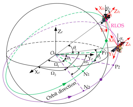
Figure 2.
Schematic of the coordination systems transformation.
The space targets orbit can be determined by the six orbital elements deriving from a given two-line element (TLE). It can be expressed as (semi-major axis), (inclination), (right ascension of the ascending node), (eccentricity), (argument of perigee), and (true anomaly) [34,35,36]. Thereafter, the accurate RLOS can be obtained by calculating the real-time position of space-based radar in the RTN coordinate system of the space target. The derivation of RLOS is as follows:
- (1)
- The positions of the space-based radar in the ECI coordinate system are given as
- (2)
- Then the coordinate transformation matrix between the ECI coordinate system and the RTN coordinate system of space target can be expressed aswhere , , , and are the orbital parameters of the space target at the k-th sample interval.
- (3)
- Thus, the position of space-based radar in the RTN coordinate system of the space target can be derived as
- (4)
- Finally, the RLOS, azimuth angle and elevation angle are calculated aswhere represents the RLOS in the space target RTN coordinate system at the k-th sample interval. and are the azimuth angle and elevation angle of the , respectively. can be utilized to calculate and to realize the dynamic RCS sequence mapping.
Considering the true anomaly can uniquely determine that the position of the space target and the orbit of low Earth orbit (LEO) satellite is close to a circle. The true anomaly of space target and of space-based radar at the k-th sample interval can be calculated by
where is the Kepler constant. and are the initial true anomaly of the space target and space-based radar, respectively.
The dynamic RLOS can be given as
Finally, the flowchart of dynamic RCS sequence mapping is shown in Figure 3.
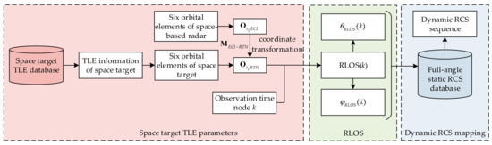
Figure 3.
Flowchart of the dynamic RCS sequence mapping.
4.2. Joint Dynamic RCS Power and Bandwidth Allocation Optimization Modeling
In this section, the Min-Max PCRLB (minimum maximum PCRLB) optimization criterion is employed to solve the power and bandwidth allocation problem in limited transmit resources of collocated MIMO radar. By fully utilizing the dynamic target RCS fluctuation characteristics, the Min-Max PCRLB optimization model can be modeled as
where and are the total transmit power and bandwidth, respectively, , , , and are the maximum power, the minimum power, the maximum bandwidth, and the minimum bandwidth of a single tracking beam, respectively, is the vector of size whose total elements is 1, represents the multi-target full-angle static RCS database, and and are the azimuth angle and elevation angle of the RLOS, respectively.
4.3. Joint Dynamic RCS Power and Bandwidth Allocation Method
It can be seen from Equations (7) and (20) that the power and bandwidth variables of space-based radar are coupled in the optimized objective function. Since the bandwidth is applied to the optimization function by squaring, the adaptive joint power and bandwidth allocation problem in this paper is a typical non-convex optimization problem. In order to solve the above problem, the C-MIMO radar bandwidth is first allocated equally, and the sub-optimal scheme of power allocation is obtained by using the convex optimization algorithm. Then the bandwidth constraint is relaxed, and finally the cyclic minimization method is used to obtain the optimal allocation results to solve the problem. The illustration of the joint dynamic RCS power and bandwidth allocation (JRPBA) method is shown in Figure 4. Additionally, the detailed process of the resource allocation method is shown in Table 1.
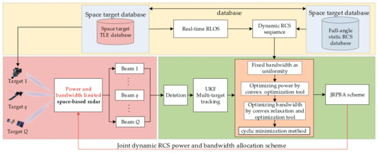
Figure 4.
Illustration of the proposed JRPBA method.

Table 1.
JRPBA method steps.
5. Simulation and Performance Evaluation
5.1. Simulation Scenario and Parameters
In the given simulation scenario, Figure 5 represents a typical multi-target tracking scenario with four space targets within the surveillance region. The space-based satellite in this scenario utilizes a C-MIMO radar system to track these four space targets. The TLE (two-line element) information [37] for the selected four space targets is depicted in Table 2. Table 3 displays the six orbital elements of the space-based radar, and Table 4 provides the radar system parameters in detail.
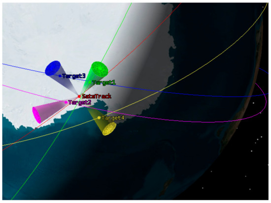
Figure 5.
Multi-target tracking simulation.
Table 2.
TLE information for the four space targets.
Table 3.
Six orbital elements of space-based radar.
Table 4.
Radar system parameters.
In the simulation experiments, the UKF (unscented Kalman filter) recursion is employed for tracking space targets using one hundred frames of radar raw data [38], with a data update rate of 1 s and 100 Monte Carlo trails. To provide a more intuitive comparison of multi-target tracking performance and tracking accuracy, the root mean square error (RMSE) of location and velocity are utilized and presented in this section.
where MC represents the total Monte Carlo trials and and are the estimated position and velocity of the i-th Monte Carlo simulation, respectively.
5.2. Dynamic RCS Sequence Mapping
In this section, the monostatic static RCS database of the space targets is calculated using electromagnetic computing software, and the simulation results are depicted in Figure 6a–d. To obtain the RLOS parameter sequences in practical applications, different methods can be employed. Here, we determine the position of satellite targets using TLE and calculate their relative position to the radar station using the SGP4 (simplified general perturbations 4) model through aerospace orbit calculation software. The RLOS parameters can then be computed using Equation (29). Finally, the dynamic RCS sequence results can be obtained by combining the static full-angle RCS and the RLOS parameters.
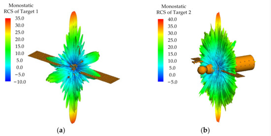
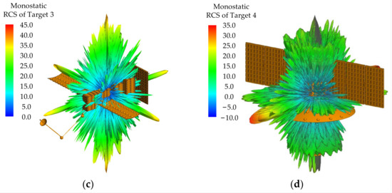
Figure 6.
Monostatic RCS of four typical space targets. (a) Static RCS of target 1. (b) Static RCS of target 2. (c) Static RCS of target 3. (d) Static RCS of target 4.
Figure 7 and Figure 8 depict the full-angle monostatic RCS of four typical space targets and the RLOS parameters of the four space targets, respectively. Figure 9 displays the dynamic RCS sequence obtained through dynamic RLOS during tracking. Upon examining Figure 7, it is evident that the fluctuation characteristics of the monostatic RCS differ among the four typical space targets as the azimuth angle varies.
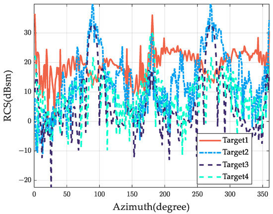
Figure 7.
Monostatic RCS of four typical space targets (azimuth degree varies from 0° to 360°, elevation degree is fixed at 90°).
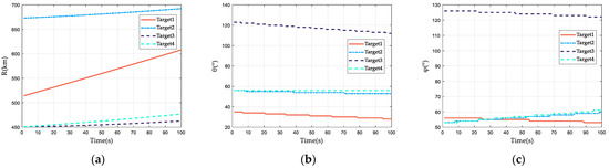
Figure 8.
Dynamic RLOS of four typical space targets. (a) Range of RLOS. (b) θ of RLOS. (c) φ of RLOS.
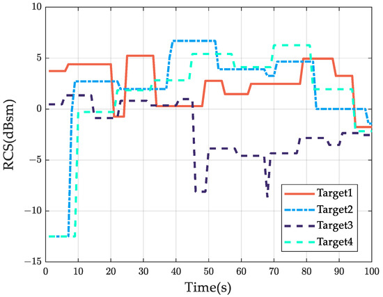
Figure 9.
Dynamic RCS sequence results.
Notice that from Figure 9 it can be observed that the dynamic RCS of different targets varies to a significant degree. The dynamic RCS of target 1 and target 2 fluctuates in a large dynamic range, while target 3 generally has the smallest RCS among the four targets. In addition, the dynamic RCS of target 1, target 2, and target 4 overlapped with each other. Therefore, the real-time dynamic RCS results can be effectively utilized to enhance the accuracy of multi-target tracking.
5.3. Joint Dynamic RCS Power and Bandwidth Allocation Method Results
Figure 10a gives the multi-target tracking result of the space targets monitored by the space-based radar. As can be seen from Figure 10b–e, the C-MIMO radar achieves multiple target tracking with simultaneous multi-beam mode. The image indicated by the arrow in Figure 10 b–e is a zoomed-in view of the region inside the red box.
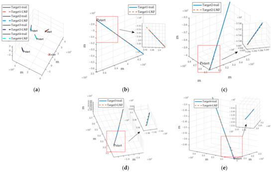
Figure 10.
Space targets tracking results. (a) Multi-target tracking. (b) Tracking result of target 1. (c) Tracking result of target 2. (d) Tracking result of target 3. (e) Tracking result of target 4.
The Min-Max PCRLB criterion is employed in this paper to dynamically allocate the power and bandwidth resource of the space-based radar. The core idea of the Min-Max PCRLB criterion is to optimize the target with the worst tracking accuracy. By solving Equation (30), the proposed method calculates the joint allocation result of power and bandwidth, as shown in Figure 11.
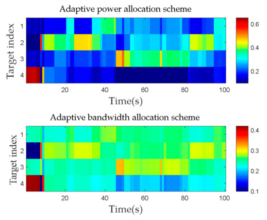
Figure 11.
Adaptive joint power and bandwidth allocation result.
As can be seen from Figure 11, the dynamic RCS of four space targets is relatively close at the tenth frame and the later tracking stage. The allocation of power and bandwidth resources in the space-based radar is influenced by the distance between the targets and the radar. As a result, targets that are located farther from the radar receive a higher allocation of radar resources. From Figure 11, it can be seen that target 2 is the farthest from the radar and the target 3 and target 4 have the closest distance. So, when the RCS of the four targets is close, the largest power bandwidth resources is allocated to target 2 and the least radar resources are allocated to target 3 and target 4.
Moreover, as the dynamic RCS of the space targets rapidly declines, the tracking accuracy of the space-based radar on these targets decreases. In order to maintain the original tracking accuracy, the proposed method allocates more system resources to the specific space target. Specifically, space target 3 receives the largest allocation of radar system resources. When tracking the 46th frame, the real-time dynamic RCS of target 3 is the smallest and to guarantee the tracking accuracy, more radar power and bandwidth resources are allocated to target 3. When tracking the 46th frame to the 82nd frame, the distance between the space-based radar and target 4 is the smallest and the dynamic RCS of target 4 is the largest, and the power and bandwidth resources allocated to target 4 are minimal. By analyzing the above simulation results, it can be seen that the distances and observation angles between the space targets play vital roles in influencing the performance of joint power and bandwidth allocation.
Figure 12 and Figure 13 depict the RMSE curves and PCRLB of position and velocity of 100 Monte Carlo experiments during the whole tracking scenario. It can be seen from Figure 12 and Figure 13 that both the ideal PCRLB for position tracking accuracy and the ideal PCRLB for velocity tracking accuracy experience a significant decrease starting from the tenth frame. Considering that the Min-Max PCRLB criterion is utilized for multi-target joint power bandwidth allocation, the PCRLB of position and the PCRLB of velocity for four space targets have the same tendency. Since the Min-Max PCRLB criterion is employed for the multi-target joint power band-width allocation, the PCRLBs for position and velocity of all four space targets exhibit a similar trend.
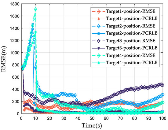
Figure 12.
The position PCRLB and RMSE of the adaptive allocation scheme.
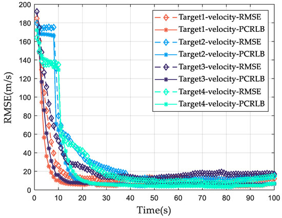
Figure 13.
The velocity PCRLB and RMSE of the adaptive allocation scheme.
It can also be seen from Figure 12 and Figure 13 that the RMSE of position and the RMSE of velocity are affected by the dynamic target RCS. Notably, when the RCS of a target decreases rapidly within a frame, the corresponding RMSE of the target’s position increases. For instance, in the 45th frame, the dynamic RCS of target 3 decreases and its corresponding tracking error increases. By optimizing the tracking performance of the target with the worst tracking accuracy, the radar power and bandwidth resources are increased to be allocated for target 3, so that the RMSE of the position estimation of target 3 decreases in the later tracking process.
5.4. Joint Power and Bandwidth Allocation Scheme Mismatch Results
To compare the multi-target tracking accuracy under different RCS models, tracking results of the traditional RCS fluctuation model and tracking results of the high dynamic RCS fluctuation adaptive joint power and bandwidth allocation are compared in this paper.
Figure 14 displays the traditional RCS fluctuation model, while Figure 15 showcases the joint power and bandwidth allocation results for multi-target tracking using this mod-el. Notice that the overall tendency of the power bandwidth allocated to the four space targets is mainly influenced by the distance between the space target and the space-based radar. Since target 2 has the greatest distance from the radar, it receives the highest allocation of radar resources. Furthermore, the RCS of four space targets is intertwined, and the radar resources obtained by the four space targets change at different times. However, the change trend is irregular and the optimal allocation of radar power and bandwidth is not formed according to the dynamic RCS fluctuation trend of space targets, which leads to the divergence of tracking error or target missing problems.
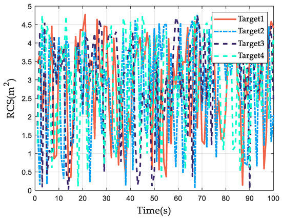
Figure 14.
The mismatched multi-target RCS.
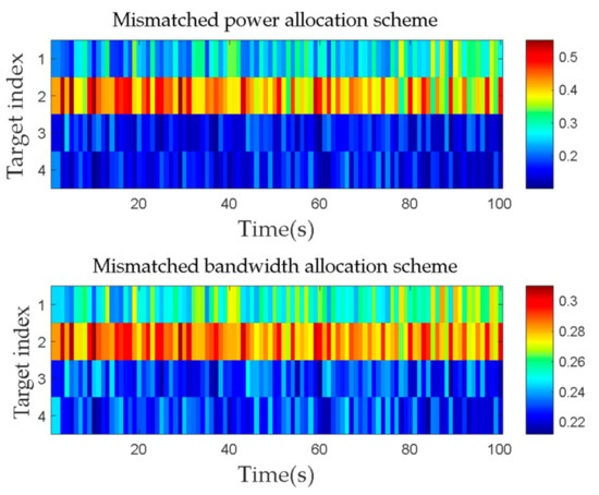
Figure 15.
Mismatched power and bandwidth allocation result.
Figure 16 and Figure 17 show the RMSE curves and PCRLBs of position and velocity with the traditional RCS fluctuation model of 100 Monte Carlo experiments, respectively.
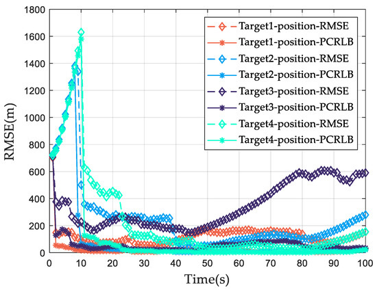
Figure 16.
The position PCRLB and RMSE of mismatched allocation result.
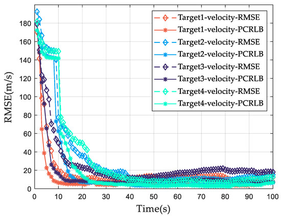
Figure 17.
The velocity PCRLB and RMSE of mismatched allocation result.
It can be clearly seen from Figure 16 and Figure 17 that while the dynamic RCS of target 3 decreases significantly at the 47th frame, the resource allocation scheme with the traditional RCS model does not change the power and bandwidth allocation ratio simultaneously, which leads to larger tracking errors for targets with smaller RCS. Under this condition, the RMSE of the position and the RMSE of the speed of target 3 are much larger than the other two targets. Consequently, it can be concluded that the traditional RCS model fails to effectively incorporate the dynamic changes in multi-target RCSs, leading to suboptimal radar power and bandwidth allocation schemes.
To show the effectiveness of the proposed method more intuitively, multi-target tracking results are compared with the high dynamic RCS model and the traditional RCS model. The comparison outcomes regarding the position RMSE and velocity RMSE are displayed in Figure 18 and Figure 19, respectively. From Figure 18, the position RMSE of target 3 is the largest, reaching 466.2 m in the 100th frame. As for the traditional RCS model, target 3 also demonstrates the largest position tracking error, showing an RMSE of 590.7 m. The proposed method shows an improved position estimation accuracy of 21.1% when compared to the traditional RCS model.
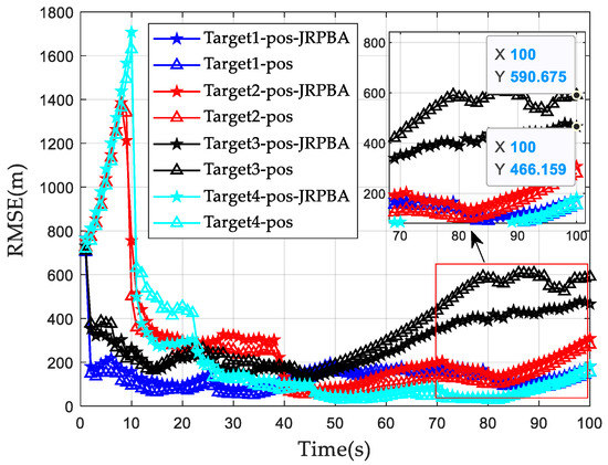
Figure 18.
Multi-target tracking position accuracy of different scheme.
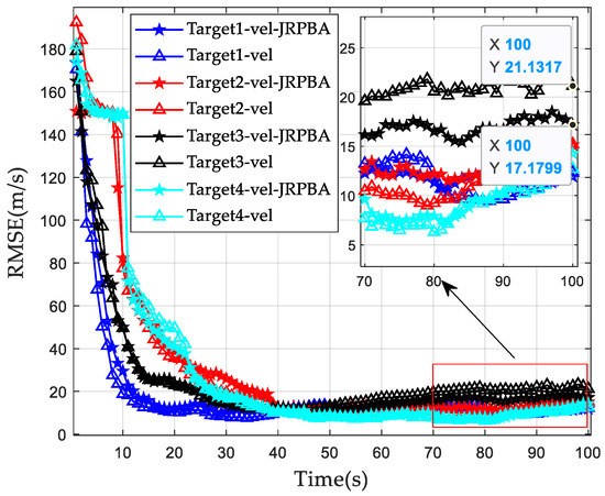
Figure 19.
Multi-target tracking velocity accuracy of different scheme.
It can be seen from Figure 19 that the traditional RCS model algorithm has the largest RMSE for target 3, reaching 21.1 m/s in the 100th frame. The RMSE of velocity obtained by the proposed method is the largest in the later tracking stage of target 3 and the corresponding value is about 17.2 m/s. The velocity estimation accuracy is improved by 18.4%. In conclusion, under the criterion of Min-Max PCRLB, the proposed method can effectively combine the real-time RCS dynamic characteristics of multiple targets in the tracking process and improve the multi-target tracking performance of the radar system.
6. Conclusions
In this paper, an adaptive joint dynamic RCS power and bandwidth allocation (JRPBA) method is proposed to solve the problem of radar tracking resources allocation in a space multi-target intersection scenario. The proposed approach establishes a mapping method between the space target motion model and the full-angle static RCS database, enabling accurate retrieval of the dynamic RCS sequence. The high dynamic characteristics of RCS are considered as prior information in the radar resource allocation framework. The optimization model, considering space multi-target RCS, power, and bandwidth, is formulated and solved using a convex relaxation method to obtain the optimal allocation scheme suitable for the actual tracking scenario. Simulation results demonstrate that compared with the traditional RCS model radar resource allocation method, the proposed JRPBA method enhances the space multi-target tracking performance and effectively resolves mismatches between the allocation scheme and the actual tracking scenario. Further research will focus on resource allocation in multi-target observation scenarios of space-based networking radar.
Author Contributions
Q.Y. proposed the conceptualization and methodology; S.Z. wrote the draft manuscript; Z.W. and L.J. supervised the experimental analysis and revised the manuscript; Y.Z. proofread and revised the first draft. All authors have read and agreed to the published version of the manuscript.
Funding
This work was funded by the National Defense Basic Scientific Research program of China, grant number WDZC20225250203.
Data Availability Statement
Not applicable.
Acknowledgments
The authors would like to thank the editors and all the reviewers for their very valuable and insightful comments during the revision of this work.
Conflicts of Interest
The authors declare no conflict of interest.
References
- Klinkrad, H. The Current Space Debris Environment and its Sources. In Space Debris: Models Risk Analysis; Springer: Berlin/Heidelberg, Germany, 2006; pp. 5–58. [Google Scholar] [CrossRef]
- Weeden, B.; Cefola, P.; Sankaran, J. Global space situational awareness sensors. In Proceedings of the Advanced Maui Optical and Space Surveillance Technologies Conference, Maui, HI, USA, 14–17 September 2010; pp. 1–10. [Google Scholar]
- Vallado, D.A.; Griesbach, J.D. Simulating Space Surveillance Networks. In Proceedings of the AAS 11-580 the AAS/AIAA Astrodynamics Specialist Conference, Napa, CA, USA, 31 July 2011; pp. 1–21. [Google Scholar]
- Delande, E.; Frueh, C.; Franco, J.; Houssineau, J.; Clark, D. Novel Multi-Object Filtering Approach for Space Situational Awareness. J. Guid. Control. Dyn. 2017, 41, 1–15. [Google Scholar] [CrossRef]
- Du, Y.; Jiang, Y.; Wang, Y.; Zhou, W.; Liu, Z. ISAR Imaging for Low-Earth-Orbit Target Based on Coherent Integrated Smoothed Generalized Cubic Phase Function. IEEE Trans. Geosci. Remote Sens. 2019, 58, 1205–1220. [Google Scholar] [CrossRef]
- Schirru, L.; Pisanu, T.; Podda, A. The Ad Hoc Back-End of the BIRALET Radar to Measure Slant-Range and Doppler Shift of Resident Space Objects. Electronics 2021, 10, 577. [Google Scholar] [CrossRef]
- Karamanavis, V.; Dirks, H.; Fuhrmann, L.; Schlichthaber, F.; Egli, N.; Patzelt, T.; Klare, J. Characterization of deorbiting satellites and space debris with radar. Adv. Space Res. 2023. [Google Scholar] [CrossRef]
- Ender, J.; Leushacke, L.; Brenner, L.; Wilden, H. RaWAdar Techniques for Space Situational Awareness. In Proceedings of the 12th International Radar Symposium (IRS), Dresden, Germany, 9–21 June 2011; pp. 1–6. [Google Scholar]
- Console, A. Command and Control of a Multinational Space Surveillance and Tracking Network; Joint Air Power Competence Centre (JAPCC): Kalkar, Germany, 2019. [Google Scholar]
- Li, J.; Stoica, P. MIMO Radar with Colocated Antennas. IEEE Signal Process Mag. 2007, 24, 106–114. [Google Scholar] [CrossRef]
- Haimovich, A.M.; Blum, R.S.; Cimini, L.J. MIMO radar with widely separated antennas. IEEE Signal Process Mag. 2008, 25, 116–129. [Google Scholar] [CrossRef]
- Cheng, Z.; Shi, S.; Tang, L.; He, Z.; Liao, B. Waveform Design for Collocated MIMO Radar With High-Mix-Low-Resolution ADCs. IEEE Trans. Signal Process 2021, 69, 28–41. [Google Scholar] [CrossRef]
- Zhang, W.W.; Shi, C.G.; Salous, S.; Zhou, J.J.; Yan, J.K. Convex optimization-based power allocation strategies for target lo-calization in distributed Hybrid non-coherent active-passive radar networks. IEEE Trans. Signal Process. 2022, 70, 2476–2488. [Google Scholar] [CrossRef]
- Xu, L.; Li, J.; Stoica, P. Target detection and parameter estimation for MIMO radar systems. IEEE Trans. Aerosp. Electron. Syst. 2008, 44, 927–939. [Google Scholar] [CrossRef]
- Garcia, N.; Haimovich, A.M.; Coulon, M. Resource allocation in MIMO radar with multiple targets for non-coherent locali-zation. IEEE Trans. Signal Process 2014, 62, 2656–2666. [Google Scholar] [CrossRef]
- Bell, K.L.; Baker, C.J.; Smith, G.E.; Johnson, J.T.; Rangaswamy, M. Cognitive Radar Framework for Target Detection and Tracking. IEEE J. Sel. Top. Signal Process 2015, 9, 1427–1439. [Google Scholar] [CrossRef]
- Yan, J.K.; Liu, H.W.; Jiu, B.; Bao, Z. Power Allocation Algorithm for Target Tracking in Unmodulated Continuous Wave Radar Network. IEEE Sensors J. 2015, 15, 1098–1108. [Google Scholar] [CrossRef]
- Yan, J.K.; Pu, W.Q.; Zhou, S.H.; Liu, H.W.; Bao, Z. Collaborative detection and power allocation framework for target tracking in multiple radar system. Inf. Fusion 2020, 55, 173–183. [Google Scholar] [CrossRef]
- Yan, J.K.; Jiu, B.; Liu, H.W.; Chen, B.; Bao, Z. Prior knowledge-based simultaneous multibeam power allocation algorithm for cog-nitive multiple targets tracking in clutter. IEEE Trans. Signal Process 2015, 63, 512–527. [Google Scholar] [CrossRef]
- Li, Z.J.; Xie, J.W.J.; Liu, W.; Zhang, H.W.; Xiang, H.H. Joint Strategy of Power and Bandwidth Allocation for Multiple Ma-neuvering Target Tracking in Cognitive MIMO Radar With Collocated Antennas. IEEE Trans. Veh. Technol. 2023, 72, 190–204. [Google Scholar] [CrossRef]
- Zhang, H.W.; Liu, W.J.; Zhang, Z.J.; Lu, W.L.; Xie, J.W. Joint Target Assignment and Power Allocation in Multiple Distributed MIMO Radar Networks. IEEE Syst. J. 2021, 15, 694–704. [Google Scholar] [CrossRef]
- Zhang, H.W.; Liu, W.J.; Xie, J.W.; Zhang, Z.J.; Lu, W.L. Joint Subarray Selection and Power Allocation for Cognitive Target Tracking in Large-Scale MIMO Radar Networks. IEEE Syst. J. 2020, 14, 2569–2580. [Google Scholar] [CrossRef]
- Zhang, H.W.; Shi, J.; Zhang, Q.; Zong, B.; Xie, J.W. Antenna Selection for Target Tracking in Collocated MIMO Radar. IEEE Trans. Aerosp. Electron. Syst. 2021, 57, 423–436. [Google Scholar] [CrossRef]
- Yi, W.; Yuan, Y.; Hoseinnezhad, R.; Kong, L. Resource Scheduling for Distributed Multi-Target Tracking in Netted Colocated MIMO Radar Systems. IEEE Trans. Signal Process 2020, 68, 1602–1617. [Google Scholar] [CrossRef]
- Tichavsky, P.; Muravchik, C.H.; Nehorai, A. Posterior Cramer-Rao bounds for discrete-time nonlinear filtering. IEEE Trans. Signal Process 1998, 46, 1386–1396. [Google Scholar] [CrossRef]
- Yuan, Y.; Yi, W.; Kirubarajan, T.; Kong, L.J. Scaled accuracy based power allocation for multi-target tracking with colocated MIMO radars. Signal Process 2019, 158, 227–240. [Google Scholar] [CrossRef]
- Xie, M.C.; Yi, W.; Kirubarajan, T.; Kong, L.-J. Joint Node Selection and Power Allocation Strategy for Multitarget Tracking in Decentralized Radar Networks. IEEE Trans. Signal Process 2018, 66, 729–743. [Google Scholar] [CrossRef]
- Grey, J.P.; Mann, I.R.; Fleischauer, M.D.; Elliott, D.G. Analytic Model for Low Earth Orbit Satellite Solar Power. IEEE Trans. Aerosp. Electron. Syst. 2020, 56, 3349–3359. [Google Scholar] [CrossRef]
- Li, Z.J.; Xie, J.W.; Ge, J.A. Power allocation optimization algorithm based on collocated MIMO radar. In Proceedings of the International Conference on Electronic Information Technology and Computer Engineering (EITCE), Xiamen, China, 18–20 October 2019; pp. 1096–1100. [Google Scholar] [CrossRef]
- Zhang, H.W.; Zong, B.; Xie, J.W. Power and Bandwidth Allocation for Multi-Target Tracking in Collocated MIMO Radar. IEEE Trans. Veh. Technol. 2020, 69, 9795–9806. [Google Scholar] [CrossRef]
- Chang, J.Y.; Fu, X.; Cheng, G.J.; Fang, G.Q.; Liu, S.L. Low-earth-orbit object detection by spaceborne netted radars. In Proceedings of the 2015 12th International Bhurban Conference on Applied Sciences and Technology (IBCAST), Islamabad, Pakistan, 13–17 January 2015. [Google Scholar]
- Challa, S.; Morelande, M.R.; Mušicki, D.; Evans, R.J. Fundamentals of Object Tracking; University Press: Cambridge, UK, 2011. [Google Scholar] [CrossRef]
- Shi, C.; Fei, W.; Zhou, J. Resource management for target tracking in distributed radar network system. In Proceedings of the IEEE International Conference on Signal Processing, Communications and Computing (ICSPCC), Zhejiang, China, 5–8 August 2015. [Google Scholar]
- Chen, J.; Fu, T.J.; Chen, D.F.J.; Gao, M.G.J. Observation angle and plane characterisation for ISAR imaging of LEO space objects. Adv. Space Res. 2016, 58, 30–44. [Google Scholar] [CrossRef]
- Ma, J.-T.; Gao, M.-G.; Guo, B.-F.; Dong, J.; Xiong, D.; Feng, Q. High resolution inverse synthetic aperture radar imaging of three-axis-stabilized space target by exploiting orbital and sparse priors. Chin. Phys. B 2017, 26, 108401. [Google Scholar] [CrossRef]
- Yu, X.; Wang, Z.; Du, X.; Jiang, L. Multipass Interferometric ISAR for Three-Dimensional Space Target Reconstruction. IEEE Trans. Geosci. Remote Sens. 2022, 60, 5110317. [Google Scholar] [CrossRef]
- Chae, H.; Kim, H.; Kwon, E.; Ryu, K.; Seong, Y.B.; Lee, J. Development of a real-time satellite orbit propagation system using TLE databases. Adv. Space Res. 2020, 66, 410–421. [Google Scholar]
- Ning, X.L.; Wang, F.; Fang, J.C. An Implicit UKF for Satellite Stellar Refraction Navigation System. IEEE Trans. Aerosp. Electron. Syst. 2017, 53, 1489–1503. [Google Scholar] [CrossRef]
Disclaimer/Publisher’s Note: The statements, opinions and data contained in all publications are solely those of the individual author(s) and contributor(s) and not of MDPI and/or the editor(s). MDPI and/or the editor(s) disclaim responsibility for any injury to people or property resulting from any ideas, methods, instructions or products referred to in the content. |
© 2023 by the authors. Licensee MDPI, Basel, Switzerland. This article is an open access article distributed under the terms and conditions of the Creative Commons Attribution (CC BY) license (https://creativecommons.org/licenses/by/4.0/).