Neural Network Compression via Low Frequency Preference

Abstract

Network pruning has been widely used in model compression techniques, and offers a promising prospect for deploying models on devices with limited resources. Nevertheless, existing pruning methods merely consider the importance of feature maps and filters in the spatial domain. In this paper, we re-consider the model characteristics and propose a novel filter pruning method that corresponds to the human visual system, termed Low Frequency Preference (LFP), in the frequency domain. It is essentially an indicator that determines the importance of a filter based on the relative low-frequency components across channels, which can be intuitively understood as a measurement of the “low-frequency components”. When the feature map of a filter has more low-frequency components than the other feature maps, it is considered more crucial and should be preserved during the pruning process. We conduct the proposed LFP on three different scales of datasets through several models and achieve superior performances. The experimental results obtained on the CIFAR datasets and ImageNet dataset demonstrate that our method significantly reduces the model size and FLOPs. The results on the UC Merced dataset show that our approach is also significant for remote sensing image classification.

1. Introduction

Deeper and wider architectures of convolutional neural networks (CNNs) have achieved great success in the field of computer vision and have been widely used in both academia and industry [1,2,3,4,5,6]. Nevertheless, they also impose high requirements for computing power and memory footprint, resulting in a significant challenge in deploying most state-of-the-art CNNs on mobile or edge devices. Therefore, reducing the parameters and calculations of existing models is still a research hot spot, where an effective technique is model compression. This technique can achieve a balanced trade-off between accuracy and model size.

Conventional compression strategies consist of network pruning [7,8,9,10,11], quantization [12,13,14], low-rank approximation [15,16], knowledge distillation [17,18,19,20] and lightweight neural framework design [21,22,23]. Network pruning has become the most popular model compression technique. Recent pruning strategies in this category can be roughly divided into weight pruning [8,24,25] and filter pruning [26,27,28], according to the granularity of pruning. Weight pruning directly removes the selected weights from a filter, resulting in unstructured sparsity. Despite the irregular structure having a high compression ratio, real acceleration cannot be achieved on general hardware platforms or Basic Linear Algebra Subprogram (BLAS) libraries [29]. Filter pruning directly discards the selected filters, leaving a regular network structure, which makes it hardware friendly. CNNs have exerted a great influence on remote sensing classification tasks with their powerful feature representation capability. Zhang et al. [30] and Volpi [31] constructed relatively small networks and trained them using satellite images from scratch. Xia et al. [32] and Marmanis et al. [33] extracted features from the middle layer of the pre-training network, formed global feature representation and realized remote sensing classification. Nogueira et al. [34] used a remote sensing dataset for fine-tuning and obtained a superior classification performance. Zhu et al. [35] proposed a knowledge-guided land pattern depicting (KGLPD) framework for urban land-use mapping. Ref. [36] constructed a new remote sensing knowledge graph (RSKG) from scratch to support the inference recognition of unseen remote sensing image scenes. Zhang et al. [37] made full use of the advantages of CNNs and CapsNet models to propose an effective framework for remote sensing image scene classification. Ref. [38] proposed a CNN pre-training method guided by the human visual attention mechanism to improve the land-use scene classification accuracy. However, the success of CNNs comes with expensive computing costs and a high memory footprint. However, the classification task of remote sensing images often needs to be carried out on the airborne or satellite-borne equipment with limited computing resources. Insufficient computing resources hinder the application of CNNs in remote sensing imaging. Therefore, model pruning technology can alleviate this resource constraint and enable CNNs to develop in the field of remote sensing. It is worth noting that the scale of public remote sensing image datasets is usually smaller than the scale of natural image datasets, which contain hundreds of thousands or even millions of images. This leads to a lot of parameter redundancy and structural redundancy in the network model, so pruning techniques are needed to reduce these redundancies and avoid overfitting of the model. Therefore, pruning technology has a great application demand and prospect in real-time remote sensing image classification (as shown in Figure 1) for resource-constrained devices such as spaceborne or airborne devices [39,40].

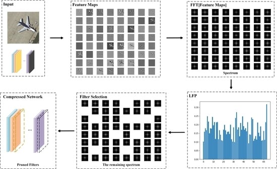
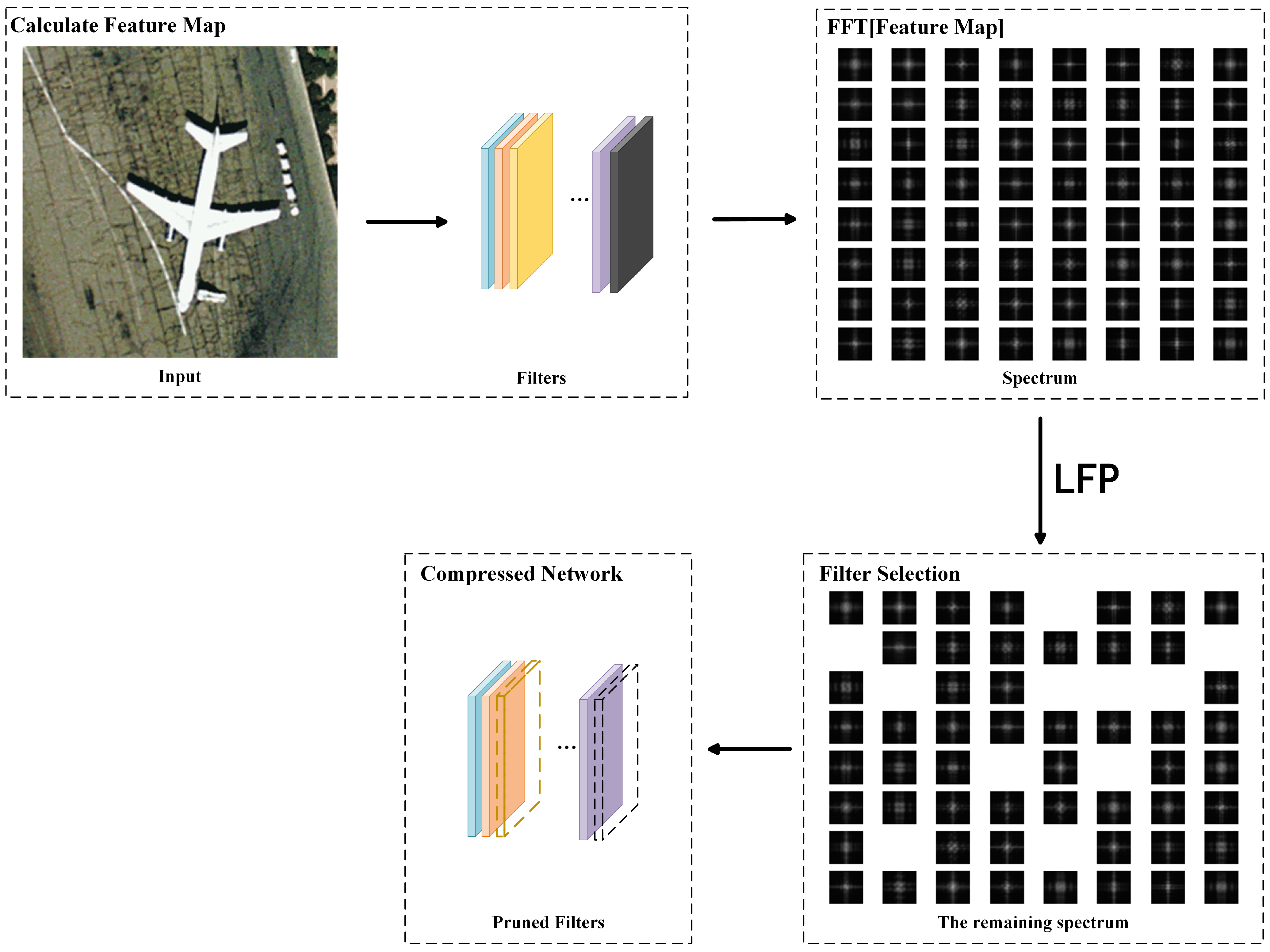
To achieve both network speedup (reduction in FLOPs) and a model size reduction (reduction in parameters), we focus on filter pruning aiming to provide a general solution (as shown in Figure 2) for devices with a low computational power.

Inherent Attribute Constraint. The pruning operation on a filter can be regarded as decreasing the constraints generated by different inherent attributes in CNNs. Li et al. [26] calculated the $L_1$-norm of parameters or features to judge the degree of attribute constraints. The conclusion was that the smaller norm, the less useful the information, which indicates that a smaller norm is a weak constraint for the network and should be pruned first. Hu et al. [41] measured the constraint of each filter by counting the Average Percentage of Zeros (APoZ) in the activation values output by the filter. The sparser the activation feature map, the weaker the constraints of the feature map. Molchanov et al. [42] used a first-order Taylor expansion to approximate the contribution of feature maps to the network output to estimate the importance of filters. He et al. [43] calculated the geometric median of filters in the same layer, in this case, the filter closest to the geometric median is considered as a weak constraint that should be pruned first. Lin et al. [44] proposed that feature maps with a lower rank have fewer constraints on the network. Therefore, the corresponding filters can be removed first. Sui et al. [45] proposed to estimate the independence of channels by calculating the nuclear norm of the feature map. Channels with a lower independence have weaker constraints and can be deleted first. In brief, these methods follow the principle of “weak constraints are pruned, strong constraints are retained” to achieve fast pruning. Nevertheless, they cannot make up for the loss in the network training process while merely improving the performance by fine-tuning in the later stage.

Induction of sparsity. These methods learn sparse structure pruning by imposing sparsity constraints on the target function in the network. Wen et al. [28] proposed a compression method based on structured sparse learning, which learns different compact structures by regularizing various network structures. Huang et al. [46] also introduced a new scaling factor, which scales the output of various structures, such as neurons, group convolutions or residual blocks, and then safely removes structures whose corresponding scaling factor is close to zero. In contrast to [46], Liu et al. [47] utilized the scaling parameter in the batch normalization layer to control the output of the corresponding channel without introducing any additional parameters. Zhao et al. [48] further extended the scaling parameters in the batch normalization layer to include bias terms and estimated their probability distributions by variational inference. These methods are not based on deterministic values but on the distribution of the corresponding scaling parameters to prune redundant channels, which makes them more interpretable. Lin et al. [49] studied important filters by incorporating two different regularizations of structural sparsity into the original loss function, achieving a superior performance on a variety of state-of-the-art network frameworks. Chen et al. [50] imposed regularizations on both filter weights and BN scaling factors and then evaluated the filter importance by their combination. Compared with the inherent attribute constraint method, the induction of sparsity achieves better compression and acceleration results. Nevertheless, the sparsity requirement must be embedded into the training process, so it is expensive with regard to training time and manpower.

In general, it is desirable to pursue a higher compression ratio and speedup ratio without losing too much accuracy. In recent years, pruning models according to the constraints provided by different inherent attributes in CNNs has become a popular filter pruning strategy. Instead of directly selecting filters, important feature maps are first determined and then the corresponding channels are retained. As reported in [44,45,51,52,53], feature maps can inherently reflect rich and important information about the input data and filters. Therefore, calculating the importance of feature maps could provide better pruning guidance for filters/channels. For example, the feature-oriented pruning concept [45] can provide richer knowledge of filter pruning than the intra-channel information when considering the correlation of multiple filter/channel feature information. The importance of a filter that is merely determined by its corresponding feature map could be easily affected by the input data. On the contrary, cross-channel feature information leads to more stable and reliable measurements, as well as a deeper exploitation of the underlying correlations between different feature maps (and corresponding filters). The results in [45] also show that the proposed inter-channel and feature-guided strategy outperforms the state-of-the-art filter-guided methods in terms of task performance (e.g., accuracy) and compression performance (e.g., model size and floating-point operation reduction).

Preference and Frequency Perspective. In previous work, both the feature-map-based strategy and the filter-guided strategy passively formulate the pruning strategy according to the inherent internal structure of CNNs in the spatial domain. Specifically, some theories, such as optimal brain damage [54] and the lottery ticket hypothesis [55,56], propose that there is parameter redundancy inside the model. Therefore, only if the parameters of the filter or feature maps are calculated in the spatial domain can their importance be determined according to experience and mathematical knowledge. Considering the “preference” of the model from the perspective of frequency domain, it can be found that the neural network often learns low-frequency information first, and then slowly learns high-frequency information [57,58] in the process of fitting the data (and some high-frequency information cannot be perfectly fitted). 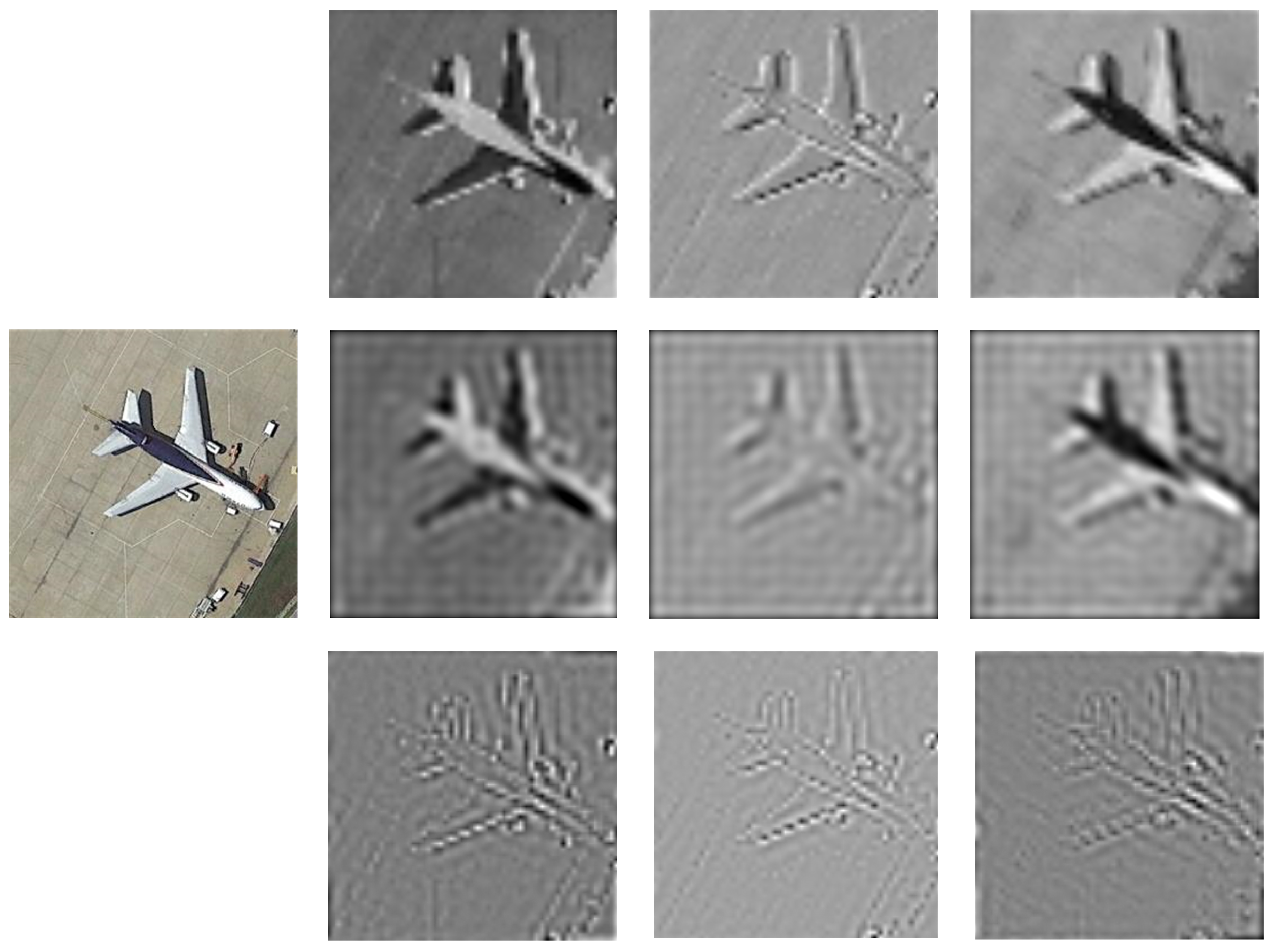At the same time, the human visual system is sensitive to the representation of low-frequency information [59,60], while the representation of low-frequency information in the spatial domain is not prominent enough. We can observe from Figure 3 that after discarding part of the high-frequency information, the category of the image can still be identified through the retained low-frequency information.

In order to maintain the consistency between the model characteristics and the human visual system, it is necessary to explore new methods in the frequency domain. Experiments in [61] show that, after adding a low-frequency filter in the test image, the robustness of the whole model is enhanced. In addition, adding low-frequency information can efficiently improve the accuracy and gradually achieve a performance similar to the original image. Considering that most real scenario images are predominantly low frequency, the influence of noise is relatively negligible on the low-frequency images but enormous on the high-frequency images, which easily leads to overfitting of the model. Therefore, a better task and compression performance can be obtained by discarding the learning of high-frequency information (the feature maps with more high-frequency components are pruned).

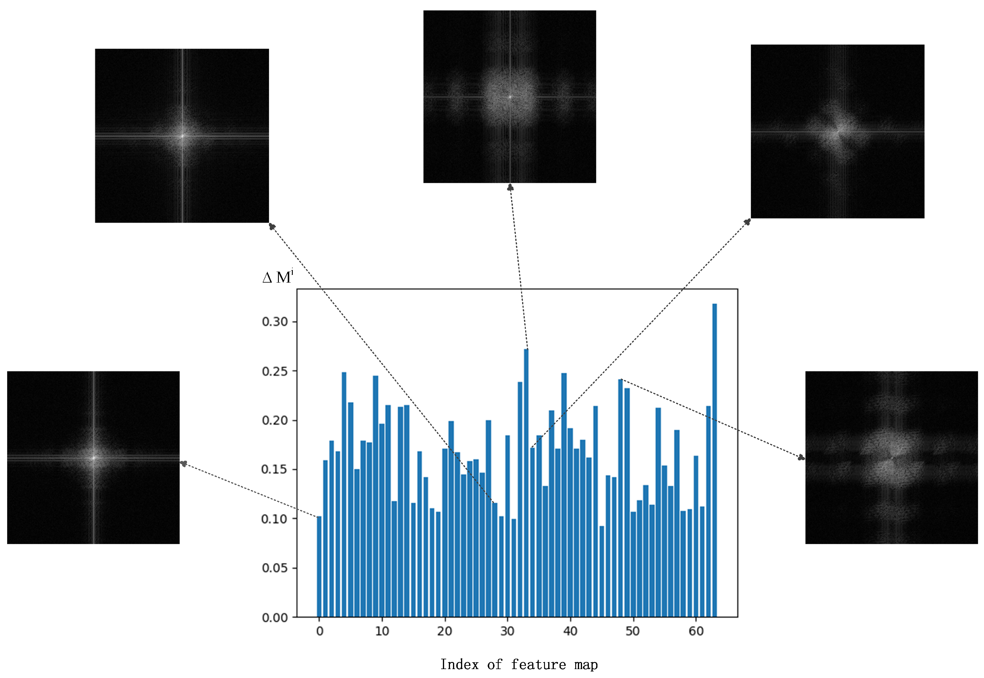
Technical Preview and Contributions. Motivated by these promising potential benefits, in this paper, we exploit the frequency information of cross-channel features for efficient filter pruning. We propose a novel metric termed Low Frequency Preference (LFP) to determine the importance of filters based on the relative frequency components across channels. It can be intuitively understood as a measurement of the “low frequency component”. Specifically, if the feature map of a filter is measured with a larger proportion of low-frequency components compared with other feature maps of the layer, the feature map is more important than that in other channels, which needs to be preserved during pruning. On the contrary, feature maps with more high-frequency components are less preferred by the model, which indicates that they contain very limited information or knowledge. Therefore, the corresponding filters are treated as unimportant and can be safely removed without affecting the model capacity.

To sum up, the contributions of this paper can be summarized as follows:

• We analyze the properties of a model from the new perspective of the frequency domain and associate the characteristics of an image with the frequency domain preference characteristics of the model. Similar to the “smaller-norm-less-important” hypothesis, we come up with a novel “lower-frequency-more-important” metric. On this basis, a low-cost, high-robustness, low-frequency component analysis scheme is proposed.
• We propose a novel metric that measures the relative low-frequency components of multiple feature maps to determine the importance of filters, termed LFP. It originates from an inter-channel perspective to determine the importance of filters more globally and precisely, thus providing better guidelines for filter pruning.
• We apply the LFP-based importance determination method to different filter pruning tasks. Extensive experiments show that the proposed method achieves good results while maintaining high precision. Notably, on the CIFAR-10 dataset, our method improves the accuracy by 0.96% and 0.95% over the baseline ResNet-56 and ResNet-110 models, respectively. Meanwhile, the model size and FLOPs are reduced by 44.7% and 48.4% (for ResNet-56) and 39.0% and 47.8% (for ResNet-110), respectively. On the ImageNet dataset, it achieves 40.8% and 46.7% storage and computation reductions, respectively, for ResNet-50 and the accuracy of Top-1 and Top-5 is 1.21% and 1.26% higher than the baseline model, respectively.

2. Proposed Method

2.1. Notation

We formally introduce symbols and notations in this section. Assume a pre-trained convolutional neural network model has L layers. We use $C_i$ and $C_{i+1}$, to represent the number of input and output channels for the i-th convolutional layer, respectively. $F_{i,j}$ represents the j-th filter of the i-th layer, then the dimension of filter is $F_{i,j}$ is ${\mathbb{R}}^{C_i\times K\times K}$, where K denotes the kernel size of the network. The i-th layer of the CNN model ${\mathcal{W}}^{\left(i\right)}$ can be represented by {$F_{i,1},F_{i,2},\dots ,F_{i,j}$} that contains j filters, where $F_{i,j}\in {\mathbb{R}}^{C_i\times K\times K}$, $1\le j\le C_{i+1}$. The tensor of connection in the deep CNN network can be parameterized by {${\mathcal{W}}^{\left(i\right)}\in {\mathbb{R}}^{C_{i+1}\times C_i\times K\times K}$, $1\le i\le L$}. The outputs of i-th layer, i.e., i-th feature maps, are denoted as ${\mathcal{M}}^i$ = {$M_{i,1},M_{i,2},\dots ,M_{i,C_{i+1}}$} ∈${\mathbb{R}}^{C_{i+1}\times h\times w}$. The feature map corresponding to the j-th channel is $M_{i,j}\in {\mathbb{R}}^h\times w$. The height and width of the feature map are h and w, respectively. In filter pruning, ${\mathcal{W}}^{\left(i\right)}$ can be split into two groups, i.e., a subset I containing $n_{i1}$ filters to be reserved and a subset, with less importance, to be pruned U containing $n_{i2}$ filters. Thus, we have $\mathit{I}\cap \mathit{U}=⌀,\mathit{I}\cup \mathit{U}={\mathcal{W}}^{\left(i\right)}$ and $n_{i1}+n_{i2}=C_{i+1}$.

2.2. Frequency Domain Analysis of Feature Maps

The Fourier transform aims to obtain the signal distribution in the frequency domain, which can also be utilized in digital image processing, since an image is a collection of points sampled in a continuous space (real scenario). It uses a two-dimensional matrix to represent each point in the space, and the image can be represented by $z=f(x,y)$. For the discrete signal of digital image, we choose the discrete Fourier transform (DFT) to obtain its frequency distribution (spectrum). Then, the frequency can be regarded as an indicator of the intensity change in the image, which reveals the gradient of the gray level in the plane space. Specifically, if the gray level changes quickly, the frequency will be high. On the contrary, if the gray level changes slowly, the frequency will be low. In terms of an image, a high-frequency signal usually corresponds to the edge and noise, while a low-frequency signal describes the image contour and background signal. The two-dimensional DFT is defined as follows:

$$\begin{array}{cc}\hfill F(u,v)& =2D-DFT\left[f\right(x,y\left)\right]\hfill \\ \hfill & =\sum _{x=0}^{M-1}\sum _{y=0}^{N-1}f(x,y)e^{-j2\pi (\frac{ux}{M}+\frac{vy}{N})},\hfill \end{array}$$

(1)

where 2D-DFT $\left[·\right]$ stands for the two-dimensional DFT; $f(x,y)$ is a digital image of size $M\times N$; and x and y are spatial variables, which, respectively, represent the specific horizontal and vertical coordinates in the digital image $f(x,y)$. Then, u and v are frequency domain variables, where $u\in \{0,1,2,\dots ,M-1\}$, $v\in \{0,1,2,\dots ,N-1\}$; $e^{-j2\pi (\frac{ux}{M}+\frac{vy}{N})}$ is the transform kernel of the DFT, which has separability.

Therefore, the DFT of the output of i-th layer (i.e., i-th feature map) is denoted as:

$$\begin{array}{cc}\hfill F_{M_{i,C_{i+1}}}(u,v)& =2D-DFT\left[M_{i,C_{i+1}}\right]\hfill \\ \hfill & =\sum _{x=0}^{h-1}\sum _{y=0}^{w-1}f(x,y)e^{-j2\pi (\frac{ux}{h}+\frac{vy}{w})},\hfill \end{array}$$

(2)

To further boost the computational efficiency of the DFT, Cooley et al. [62] proposed a special kind of DFT termed a one-dimensional fast Fourier transform (FFT). In this way, the number of multiplications required in the DFT can be greatly reduced. In addition, the more sampling points to be transformed, the more significant the savings of the FFT algorithm computation. Based on the separability of the Fourier transform kernel $e^{-j2\pi (\frac{ux}{h}+\frac{vy}{w})}$, the 2D-DFT can also be computed using the two-step FFT:

$$\begin{array}{cc}\hfill F_{M_{i,C_{i+1}}}(u,v)& =FF{T}_x\left\{FF{T}_y\left[f(x,y)\right]\right\}\hfill \\ \hfill & =FF{T}_y\left\{FF{T}_x\left[f(x,y)\right]\right\}\hfill \\ \hfill & =FFT\left(M_{i,C_{i+1}}\right),\hfill \end{array}$$

(3)

The spectrum map obtained by the two-dimensional Fourier transform is a distribution of image gradient. The points on the spectrum map do not have a one-to-one correspondence with the points on the image plane, even if the frequency is not shifted. The degree of brightness or darkness on the Fourier spectrum map indicates the intensity difference between the gray value of a point on the image with the neighboring points (i.e., the gradient and the frequency value of a point). Larger differences/gradients indicate higher frequencies and lower energies, which leads to lower values and a darker appearance on the spectrum map. A smaller difference/gradient indicates a lower frequency and a higher energy, resulting in a higher numerical value and a brighter appearance on the spectrum map. In other words, the brighter the frequency spectrum, the higher the energy, the lower the frequency and the smaller the image difference (more flat). Therefore, the result of the FFT on the image is shown in Figure 4c. The low-frequency component of the image is distributed in the four corners of the spectrum map. For better observation, the low-frequency component $F(0,0)$ is translated to the center of the frequency rectangle defined by the interval $[0,M-1]$ and $[0,N-1]$ via the following equation:

$$f(x,y){(-1)}^{x+y}\stackrel{FFT}{⟶}F(u-\frac{M}{2},v-\frac{N}{2}),$$

(4)

In the displayed spectrum map, since the dynamic range of other gray values is compressed, the log transformation in Equation (5) is performed once on Figure 4c,d. Therefore, the details can be greatly improved to observe and calculate the spectral law.

$$F^{\prime }(u,v)=1+log\left|F(u,v)\right|,$$

(5)

Therefore, the i-th spectrum map (the i-th feature map after FFT) is represented as ${\mathcal{M}}_{FFT}^i$ = {$M_{i,1}^F,M_{i,2}^F,\dots ,M_{i,C_{i+1}}^F$}. To observe the extraction of different frequency features by different filters more apparently, we visualize the feature maps of the model ResNet-50-conv1 as well as the corresponding spectrum map in Figure 5 and Figure 6. The bright areas in the spectrum correspond to the low-frequency components (with higher values), while the dark areas correspond to the high-frequency components (with lower values). In addition, some spectra with fewer low-frequency components and the corresponding feature maps are annotated with red boxes. Therefore, we can prune the filters corresponding to the feature maps with fewer low-frequency components, thus leaving more low-frequency components.

2.3. LFP-Based Model Pruning

As mentioned above, measuring importance in the frequency domain is a new research approach. Motivated by those promising benefits in Section 1, we propose to explore the filter importance from an inter-channel perspective, and the key idea is to use LFP to measure the importance of each feature map (and its corresponding filter). Specifically, if there are more low-frequency components in a feature map of a channel, the model “prefers” its intrinsic information, that is to say, the Frequency Preference Index of this feature map is higher. The Frequency Preference Index is higher as the filter corresponding to the feature map becomes more important. On the other hand, feature maps with relatively few low-frequency components (i.e., high-frequency components dominate) contain relatively little useful information. Therefore, even if the corresponding filter is excluded, the information and knowledge can still be roughly preserved by feature maps of other filters after the fine-tuning process. In other words, filters that generate low-frequency preference feature maps tend to be more “ignorable”, which can be interpreted as having lower importance. Therefore, it would be appropriate to remove those filters that have feature maps with low channel frequency preferences, while still maintaining the high model capacity.

Filter pruning aims to identify and remove the less important filter sets from ${\mathcal{W}}^{\left(i\right)}$. To accurately measure the importance, we design a mathematical metric to quantify the Frequency Preference of a feature map using the Frobenius norm in Equation (6). It was reported in [63,64] that the F-norm can be used to measure the energy and difference of an image. In addition, we have also mentioned that higher frequency locations in the image mean lower energy, lower value, and a darker appearance in the spectrum. On the contrary, lower frequency locations mean higher energy, higher values and a brighter appearance on the spectrum. To this end, we elaborate a mathematical metric to measure Frequency Preference by using the F-norm of the spectrum.

$${∥A∥}_F=\sqrt{tr\left(A^{T}A\right)}=\sqrt{\sum _{i=1}^m\sum _{j=1}^n{\left|a_{ij}\right|}^2},$$

(6)

where A is an $m\times n$ matrix and $a_{ij}$ is each element of matrix A.

If the importance of a filter is merely determined by its corresponding feature map, the results may be sensitive to input data. Cross-channel feature information leads to more stable and reliable measurements, which is suitable for discovering the underlying correlations between different feature maps (and corresponding filters). Thus, in practice, in order to simultaneously remove multiple unimportant filters, a combination of frequency preference on multiple feature maps needs to be calculated. For the i-th layer with output feature maps, ${\mathcal{M}}_{FFT}^i$ = {$M_{i,1}^F,M_{i,2}^F,\dots ,M_{i,C_{i+1}}^F$}∈${\mathbb{R}}^{C_{i+1}\times h\times w}$. Firstly, let ${\mathcal{M}}_{FFT}^i$ be rewritten as $M^i={[{m_{i,1}}^T,{m_{i,2}}^T,\dots ,{m_{i,C_{i+1}}}^T]}^T$∈${\mathbb{R}}^{C_{i+1}\times hw}$, a matrix of $C_{i+1}$ rows and $hw$ columns, $m_{i,C_{i+1}}\in {\mathbb{R}}^{hw}$. To determine the minimum k-row frequency preference in ${\mathcal{M}}_{FFT}^i$, we first successively delete row $m_{i,j}$ from $M^i$ and compute the corresponding F-norm change between the remaining ($C_{i+1}-1$) row matrix and the original $C_{i+1}$ row matrix $M^i$. Then, $C_{i+1}$ F-norm change values are obtained after $C_{i+1}$ computations, and the k values with the smallest change are determined by sorting, along with their corresponding feature maps. These selected k feature maps $M_{i,j}$ are interpreted as receiving a lower “preference” from the model compared to other feature maps, so their corresponding filters $F_{i,j}$ are less important and should be pruned. Therefore, computing the change in the global F-norm in the feature map ${\mathcal{M}}^i$ in i-th layer, that is, the low frequency preference of ${\mathcal{M}}^i$, can be defined as follows:

$$LFP\left[{\mathcal{M}}^i\right]\triangleq {[{∥M^i∥}_F-{∥M^i\ast Z_j∥}_F]}_{j=1}^{C_{i+1}},$$

(7)

where ${∥·∥}_F$ is the Frobenius norm, ∗ is the matrix convolution operation and $Z_j$ is the row mask matrix whose j-th row entries are zeros and other entries are ones.

In the set of F-norm changes obtained by LFP$\left[{\mathcal{M}}^i\right]$, the k smallest changes can be determined according to the pruning rate, and the corresponding feature maps and filters are not important and can be pruned. As shown in Figure 7, by randomly extracting the spectra corresponding to five change values, it can be observed that the spectra with more low-frequency components show higher LFP change values.

2.4. The Overall Algorithm

Combining the above two steps, the whole filter pruning process is developed from an inter-channel perspective. Figure 8 is a chart of methodology for the proposed method. The pseudo-code of LFP is provided in Algorithm 1, which gives a lucid description and summary of our proposed filter pruning algorithm. Starting from a pre-trained model ${\mathcal{W}}^{\left(i\right)}$, the feature maps obtained after the image input model are calculated by the FFT to obtain the spectrum. The spectrum is reshaped into a matrix $M^i$ with row $C_{i+1}$ and column $hw$. Then, an LFP calculation is performed on $M^i$ and the results are sorted. According to the pruning ratio, specific filters can be pruned. After fine-tuning the pruned model, a sub-model ${\mathcal{W}}^{\ast }$ can be obtained.

Algorithm 1 Algorithm Description of the LFP method for the i-th layer

Input:  An L-layer CNN model with pre-trained weights ${\mathcal{W}}^{\left(i\right)}$; The i-th feature maps ${\mathcal{M}}^i$ = {$M_{i,1},M_{i,2},\dots ,M_{i,C_{i+1}}$} ∈${\mathbb{R}}^{C_{i+1}\times h\times w}$; target sparsity S; training set D; Output:  A sub-model satisfying the target sparsity S and its optimal weight values ${\mathcal{W}}^{*}$; 1: for Sample a mini-batch from D do 2:     FFT calculation: Calculate $F_{M_i,C_{i+1}}$ by Equation  (3) 3:     Reshape FFT feature maps: $M^i:=reshape({\mathcal{M}}_{FFT}^i,[C_{i+1},hw])$ 4:     for $i=1$; $i<=C_{i+1}$; $i++$ do 5:         LFP calculation: LFP[${\mathcal{M}}^i$] by Equation  (7) 6:     end for 7: end for 8: Filters Selection: Sort LFP[${\mathcal{M}}^i$]; 9: Pruning: Prune $S\times C_{i+1}$ filters via the $S\times C_{i+1}$ smallest LFP[${\mathcal{M}}^i$]; 10: Fine-tuning;

3. Experiments and Analysis

3.1. Experimental Settings

Baselines Models and Datasets. To demonstrate the effectiveness and generality of the proposed LFP method, we evaluate its pruning performance against various baseline models on three image classification datasets. Specifically, we introduce LFP into three modern CNN models (ResNet-56 [65], ResNet-110 [65] and VGG-16 [66]) on the CIFAR-10 dataset [67] and ResNet-20 [65] on the CIFAR-100 [67] dataset. CIFAR-10 contains 60,000 color images (50,000 for training and 10,000 for testing) with a uniform size of 32 × 32 and classes of 10, but CIFAR-100 has 100 classes. In addition, we further evaluate and compare the performance with other state-of-the-art pruning methods using the ResNet-50 model [65] on ImageNet [68], which is a large-scale and challenging dataset. In addition, we perform our algorithm on VGG-16 with a publicly available dataset designed for remote sensing image classification, called UC Merced land-use dataset, which consists of images of 21 land-use scene categories [69]. Each class contains 100 images with the size of 256 × 256 pixels and a one foot spatial resolution. Figure 9 shows some example images randomly selected from the UC Merced dataset.

Configurations. We use PyTorch 1.6.0, Python 3.7 and CUDA 10.2 for implementation and thop for calculating the parameters and FLOPs. Referring to the experimental design in [44,45], an identical layer-by-layer pruning strategy is adopted in our framework. To determine the LFP of each filter, we randomly sample five batches (total five × mini-batch input images) to calculate the average LFP of each feature map in all the experiments. After completing filter pruning based on LFP, we perform fine-tuning on the pruned models with stochastic gradient descent (SGD) [70,71,72] as the optimizer. SGD can more efficiently use information, especially when the information is more redundant [72,73,74]. In addition, we perform the fine-tuning for 300 epochs on CIFAR and UC Merced datasets with the batch size 256, momentum of 0.9, weight decay of 0.005 and initial learning of 0.01. On the ImageNet dataset, fine-tuning is performed for 150 epochs with the batch size of 128, momentum of 0.99, weight decay of 0.0001 and initial learning rate of 0.1.

3.2. Results on CIFAR Datasets

To prove the feasibility of LFP, we use different pruning ratios (

Table 1. Pruning ratio of various baseline models on different datasets by LFP.

Model/Dataset	Pruning Ratio Setting of All Layers
ResNet-56/CIFAR-10	[0.0] + [0.15] × 2 + [0.4] × 27
	[0.0] + [0.4] × 2 + [0.5] × 9 + [0.6] × 9 + [0.7] × 9
ResNet-110/CIFAR-10	[0.0] + [0.2] × 2 + [0.3] × 18 + [0.35] × 36
	[0.0] + [0.4] × 2 + [0.5] × 18 + [0.65] × 36
VGG-16/CIFAR-10	[0.3] × 7 + [0.75] × 5
	[0.45] × 7 + [0.78] × 5
ResNet-20/CIFAR-100	[0.0] + [0.1] × 2 + [0.25] × 9
	[0.0] + [0.3] × 2 + [0.3] × 3 + [0.4] × 3 + [0.5] × 3
ResNet-50/ImageNet	[0.0] + [0.1] × 3 + [0.35] × 16
	[0.0] + [0.5] × 3 + [0.6] × 16

) to achieve the goal of high accuracy, as well as the goals of model size and FLOP reduction.

Table 2. Pruning results of ResNet-56 on the CIFAR-10 dataset.

Method	Pruned Top-1%	$\mathbf{\Delta }$ Top-1	Parameters (↓%)	FLOP (↓%)
ResNet-56 [65]	93.26	0	0.85M (0.0)	125.49M (0.0)
L1-norm [26]	93.06	−0.20	0.73M (14.1)	90.90M (27.6)
NISP [75]	93.01	−0.25	0.49M (42.4)	81.00M (35.5)
GAL-0.6 [76]	92.98	−0.28	0.75M (11.8)	78.30M (37.6)
HRank [44]	93.52	+0.26	0.71M (16.8)	88.72M (29.3)
CHIP [45]	94.16	+0.90	0.48M (43.5)	65.94M (47.5)
RUFP [77]	93.57	+0.52	0.52M (38.8)	79.3M (37.6)
LFP (Ours)	94.22	+0.96	0.47M (44.7)	64.71M (48.4)
GAL-0.8 [76]	91.58	−1.68	0.29M (65.9)	49.99M (60.2)
LASSO [78]	91.80	−1.46	N/A	62.00M (50.6)
HRank [44]	90.72	−2.54	0.27M (68.1)	32.52M (74.1)
CHIP [45]	92.05	−1.21	0.24M (71.8)	34.79M (72.3)
LFP (Ours)	92.70	−0.56	0.24M (71.8)	35.37M (71.8)

,

Table 3. Pruning results of ResNet-110 on the CIFAR-10 dataset.

Method	Pruned Top-1%	$\mathbf{\Delta }$ Top-1	Parameters (↓%)	FLOPs (↓%)
ResNet-110 [65]	93.50	0	1.72M (0.0)	252.89M (0.0)
L1-norm [26]	93.30	−0.20	1.16M (32.6)	155.00M (38.7)
HRank [44]	94.23	+0.73	1.04M (39.5)	148.70M (41.2)
CHIP [45]	94.44	+0.94	0.89M (48.3)	121.09M (52.1)
LFP (Ours)	94.45	+0.95	1.05M (39.0)	132.08M (47.8)
GAL-0.5 [76]	92.74	−0.76	0.95M (44.8)	130.20M (48.5)
HRank [44]	92.65	−0.85	0.53M (69.2)	79.30M (68.6)
CHIP [45]	93.63	+0.13	0.53M (69.2)	71.69M (71.6)
LFP (Ours)	93.72	+0.22	0.54M (68.6)	72.83M (71.2)

,

Table 4. Pruning results of VGG-16 on the CIFAR-10 dataset.

Method	Pruned Top-1%	$\mathbf{\Delta }$ Top-1	Parameters (↓%)	FLOPs (↓%)
VGG-16 [66]	93.96	0	15.00M (0.0)	314.00M (0.0)
SSS [46]	93.02	−0.94	3.93M (73.8)	183.13M (41.6)
GAL-0.05 [76]	93.77	−0.19	3.36M (77.6)	189.49M (39.6)
HRank [44]	93.43	−0.53	2.51M (83.3)	145.61M (53.6)
CHIP [45]	93.86	−0.10	2.76M (81.6)	131.17M (58.1)
RUFP [77]	93.81	−0.15	2.50M (83.3)	167.00M (46.8)
LFP (Ours)	93.98	+0.02	2.51M (83.3)	104.96M (66.6)
GAL-0.1 [76]	93.42	−0.54	2.67M (82.2)	171.89M (45.2)
HRank [44]	91.23	−2.73	1.78M (92.0)	73.70M (76.5)
CHIP [45]	93.18	−0.78	1.90M (87.3)	66.95M (78.7)
LFP (Ours)	93.61	−0.35	1.89M (87.4)	67.09M (78.6)

and

Table 5. Pruning results of ResNet-20 on the CIFAR-100 dataset.

Method	Pruned Top-1%	$\mathbf{\Delta }$ Top-1	Parameters (↓%)	FLOPs (↓%)
ResNet-20 [65]	68.47	0	278.3k (0.0)	41.20M (0.0)
L1-norm [26]	66.59	−1.88	176.2k (36.7)	20.80M (49.5)
L2-norm [79]	66.61	−1.86	175.9k (36.8)	21.00M (49.0)
FPGM-0.4 [43]	66.68	−1.79	183.8k (34.0)	20.60M (50.0)
PFP [80]	66.19	−2.28	176.3k (36.7)	21.00M (49.0)
KLNP [81]	66.68	−1.79	187.5k (32.7)	21.20M (48.5)
LFP (Ours)	67.43	−1.04	175.8k (36.7)	20.62M (50.0)
IENP [27]	65.76	−2.71	168.8k (39.4)	20.00M (51.5)
LFP (Ours)	65.82	−2.65	157.4k (43.4)	19.65M (52.3)

show the evaluation results of the pruned modern CNN models on the CIFAR-10/100 datasets, respectively.

For the ResNet-56 model, our LFP-based method improves the accuracy by 0.96% over the baseline model, and reduces the model size and FLOPs by 44.7% and 48.4%, respectively. When the model size and FLOPs are both reduced by 71.8%, we still achieve a better performance.

For the ResNet-110 model, the accuracy is improved by 0.95% and the model size and FLOP are reduced by 39.0% and 47.8%, respectively. When the model size and FLOP are reduced by 68.6% and 71.2% for pruning (close to the highest compression ratio of the algorithm), our pruned model can still obtain a 0.22% accuracy improvement over the baseline model.

For the VGG-16 model, our method can reduce the model size and FLOPs by 83.3% and 66.6%, respectively. Meanwhile, it still improves the accuracy by 0.02%. In addition, when the compression ratio of the pruned model is close to [44,45], the storage and computational cost are reduced by 87.4% and 78.6%, respectively, and the accuracy is merely reduced by 0.35%.

For the ResNet-20 model on CIFAR-100, on the premise of little accuracy loss, LFP can reduce the model size and FLOP by 36.7% and 50.0%, respectively. When the model is further compressed, the accuracy of our method is reduced by only 2.65%.

After preliminary pruning on ResNet-56/110 and VGG-16, LFP can be more accurate than the baseline model. This shows that the LFP algorithm can alleviate the overfitting problem of the original model while reducing the model size and calculation costs. Although further pruning on ResNet-56 and VGG-16 will cause a slight drop in accuracy, it is within an acceptable range compared to other algorithms.

3.3. Results on ImageNet

The proposed LFP not only shows good performance on small datasets but works well on large-scale datasets. To verify the effectiveness more comprehensively, we also conducted several experiments on the challenging ImageNet dataset.

Table 6. Pruning results of ResNet-50 on the ImageNet dataset.

Method	Pruned Top-1%	$\mathbf{\Delta }$ Top-1	Pruned Top-5%	$\mathbf{\Delta }$ Top-5	Parameters (↓%)	FLOPs (↓%)
ResNet-50 [65]	76.15	0	92.87	0	25.50M (0.0)	4.09B (0.0)
ThiNet [83]	72.04	−4.11	90.67	−2.20	16.91M (33.7)	2.58B (36.8)
SFP [84]	74.61	−1.54	92.06	−0.81	N/A	2.38B (41.8)
Auto [85]	74.76	−1.39	92.15	−0.72	N/A	2.10B (48.7)
GAL-0.5 [76]	71.95	−4.20	90.94	−1.93	21.19M (16.9)	2.33B (43.0)
FPGM-0.3 [43]	75.59	−0.56	92.63	−0.24	15.94M (37.5)	2.36B (42.2)
HRank [44]	74.98	−1.17	92.33	−0.54	16.17M (36.6)	2.30B (43.7)
SCOP-0.4 [52]	75.95	−0.20	92.79	−0.08	14.59M (42.8)	2.24B (45.3)
CHIP [45]	76.30	+0.15	93.02	+0.15	15.10M (40.8)	2.26B (44.8)
CHEX-0.3 [82]	77.40	+1.25	N/A	-	N/A	2.00B (51.1)
LFP (Ours)	77.36	+1.21	94.13	+1.26	15.09M (40.8)	2.18B (46.7)
PFP [80]	75.21	−0.94	92.43	−0.44	17.82M (30.1)	2.29B (44.0)
SCOP-0.5 [52]	75.26	−0.89	92.53	−0.34	12.29M (51.8)	1.86B (54.6)
CHIP [45]	75.26	−0.89	92.53	−0.34	11.04M (56.7)	1.52B (62.8)
CHEX-0.5 [82]	76.00	−0.15	N/A	-	N/A	1.00B (75.6)
LFP (Ours)	76.07	−0.08	92.26	+0.09	8.02M (68.5)	0.97B (76.3)

lists the pruning performance of ResNet-50 on the ImageNet dataset via our method. The results indicate that, when targeting a small compression ratio, our method can achieve 40.8% and 46.7% storage and computation reductions, respectively. In addition, the accuracy of top-1 and top-5 is 1.21% and 1.26% higher than the baseline model, respectively. When the compression ratio is further increased, LFP still achieves a superior performance over the state-of-the-art methods. That is, the accuracy can be guaranteed while maintaining a high compression ratio. However, in the case of a small compression ratio, CHEX [82] is slightly more accurate than LFP. At the same time, the reductions in model size and computation are not optimal for LFP. However, in the further compression, LFP shows its superiority in precision, storage and computation reduction.

3.4. Results on the UC Merced Dataset

Table 7. Pruning results of VGG-16 on the UC Merced land-use dataset.

Method	Pruned Top-1%	$\mathbf{\Delta }$ Top-1	Parameters (↓%)	FLOPs (↓%)
VGG-16 [66]	93.45	0	15.00M (0.0)	314.00M (0.0)
LFP (Ours)	93.68	+0.23	3.25M (78.3)	186.61M (40.6)
LFP (Ours)	92.77	−0.68	2.04M (86.4)	146.53M (53.3)

lists the pruning performance of VGG-16 on the UCM dataset via our method. The experimental results show that the proposed LFP also performs well in remote sensing image classification. When targeting a small compression ratio, our method can achieve 78.3% and 40.6% storage and computation reductions, respectively. Meanwhile, the accuracy is 0.23% higher than the baseline model. It can be seen that LFP has a tiny loss in accuracy (it decreases by 0.68) when the compression ratio is further increased. That is, the accuracy can be guaranteed while maintaining a high compression ratio.

4. Discussion

This paper proposes a novel model compression method for frequency domain filtering in accordance with the “smaller-norm-less-important” idea. In contrast to previous algorithms that perform pruning in the spatial domain, we explore the similarity, symmetry and substitutability of feature maps. We re-consider the model characteristics that correspond to the human visual system termed Low Frequency Preference (LFP) in the frequency domain. Based on the new frequency domain perspective and model characteristics, the performance of LFP is even superior to state-of-the-art methods [45,82].

Although our LFP is originally proposed for CNNs, there are few pruning algorithms for recurrent neural networks (RNNs). However, we are working hard to explore this limitation, and hope to extend the pruning algorithm to more diverse network structures in the future. Secondly, although it is effective to utilize F-norm pruning in the pruning process, whether there is a more appropriate and accurate metric for pruning than F-norm will continue to be explored in future work. At the same time, we will also focus on the study of different pruning granularities such as [71] to further compress the model.

5. Conclusions

Convolutional neural networks (CNNs) have been widely used in remote sensing image classification due to their powerful feature representation abilities. However, the accompanying high computational cost is always a problem worth trying to improve. In this paper, we propose a novel pruning method called low frequency preference (LFP) from the new perspective of the frequency domain, which takes into account the model properties (i.e., the preference of the network model) for the data properties. It determines the relative importance of filters by observing and computing the spectrogram of the feature map. We conducted LFP with several modern and popular models on different scale datasets to verify its superiority. The experimental results demonstrate that the LFP pruning method can effectively reduce the computational complexity and model size while maintaining a high classification accuracy.

In future research, we will continue to explore different pruning methods in the frequency domain, as well as combine the spatial domain pruning methods to achieve a higher compression ratio. The goal is to find a method to prune CNNs from scratch for remote sensing image classification. Since the pruned channels are already selected when training the original over-parameterized network, pruning CNNs from scratch can save more computational resources and time. It is also of great significance for resource-constrained remote sensing image classification tasks.

References

1. Long, J.; Shelhamer, E.; Darrell, T. Fully convolutional networks for semantic segmentation. In Proceedings of the IEEE Conference on Computer Vision and Pattern Recognition (CVPR), Boston, MA, USA, 7–12 June 2015; pp. 3431–3440. [Google Scholar]
2. Girshick, R.; Donahue, J.; Darrell, T.; Malik, J. Rich feature hierarchies for accurate object detection and semantic segmentation. In Proceedings of the IEEE Conference on Computer Vision and Pattern Recognition, Columbus, OH, USA, 23–28 June 2014; pp. 580–587. [Google Scholar]
3. Girshick, R. Fast r-cnn. In Proceedings of the IEEE International Conference on Computer Vision (ICCV), Santiago, Chile, 7–13 December 2015; pp. 1440–1448. [Google Scholar]
4. Ren, S.; He, K.; Girshick, R.; Sun, J. Faster r-cnn: Towards real-time object detection with region proposal networks. Adv. Neural Inf. Process. Syst. 2015, 28, 91–99. [Google Scholar] [CrossRef] [PubMed] [Green Version]
5. He, K.; Gkioxari, G.; Dollár, P.; Girshick, R. Mask r-cnn. In Proceedings of the IEEE International Conference on Computer Vision (ICCV), Venice, Italy, 22–29 October 2017; pp. 2961–2969. [Google Scholar]
6. Chen, L.C.; Papandreou, G.; Kokkinos, I.; Murphy, K.; Yuille, A.L. Deeplab: Semantic image segmentation with deep convolutional nets, atrous convolution, and fully connected crfs. IEEE Trans. Pattern Anal. Mach. Intell. 2017, 40, 834–848. [Google Scholar] [CrossRef] [PubMed] [Green Version]
7. Blalock, D.; Gonzalez Ortiz, J.J.; Frankle, J.; Guttag, J. What is the state of neural network pruning? Proc. Mach. Learn. Syst. 2020, 2, 129–146. [Google Scholar]
8. Han, S.; Mao, H.; Dally, W.J. Deep compression: Compressing deep neural networks with pruning, trained quantization and huffman coding. arXiv 2015, arXiv:1510.00149. [Google Scholar]
9. Deng, C.; Liao, S.; Yuan, B. Permcnn: Energy-efficient convolutional neural network hardware architecture with permuted diagonal structure. IEEE Trans. Comput. 2020, 70, 163–173. [Google Scholar] [CrossRef]
10. Liang, T.; Glossner, J.; Wang, L.; Shi, S.; Zhang, X. Pruning and quantization for deep neural network acceleration: A survey. Neurocomputing 2021, 461, 370–403. [Google Scholar] [CrossRef]
11. Xu, K.; Zhang, D.; An, J.; Liu, L.; Liu, L.; Wang, D. GenExp: Multi-objective pruning for deep neural network based on genetic algorithm. Neurocomputing 2021, 451, 81–94. [Google Scholar] [CrossRef]
12. Esser, S.K.; McKinstry, J.L.; Bablani, D.; Appuswamy, R.; Modha, D.S. Learned step size quantization. arXiv 2019, arXiv:1902.08153. [Google Scholar]
13. Xu, Y.; Wang, Y.; Zhou, A.; Lin, W.; Xiong, H. Deep neural network compression with single and multiple level quantization. In Proceedings of the AAAI Conference on Artificial Intelligence, New Orleans, LO, USA, 2–7 February 2018; Volume 32. [Google Scholar]
14. Rastegari, M.; Ordonez, V.; Redmon, J.; Farhadi, A. Xnor-net: Imagenet classification using binary convolutional neural networks. In European Conference on Computer Vision ECCV 2016; Springer: Berlin/Heidelberg, Germany, 2016; pp. 525–542. [Google Scholar]
15. Pan, Y.; Xu, J.; Wang, M.; Ye, J.; Wang, F.; Bai, K.; Xu, Z. Compressing recurrent neural networks with tensor ring for action recognition. In Proceedings of the AAAI Conference on Artificial Intelligence, Honolulu, HI, USA, 27 January–1 February 2019; Volume 33, pp. 4683–4690. [Google Scholar]
16. Yin, M.; Sui, Y.; Liao, S.; Yuan, B. Towards efficient tensor decomposition-based dnn model compression with optimization framework. In Proceedings of the IEEE/CVF Conference on Computer Vision and Pattern Recognition, Nashville, TN, USA, 20–25 June 2021; pp. 10674–10683. [Google Scholar]
17. Park, W.; Kim, D.; Lu, Y.; Cho, M. Relational knowledge distillation. In Proceedings of the IEEE/CVF Conference on Computer Vision and Pattern Recognition, Long Beach, CA, USA, 15–20 June 2019; pp. 3967–3976. [Google Scholar]
18. Hinton, G.; Vinyals, O.; Dean, J. Distilling the knowledge in a neural network. arXiv 2015, arXiv:1503.02531. [Google Scholar]
19. Zhang, L.; Song, J.; Gao, A.; Chen, J.; Bao, C.; Ma, K. Be your own teacher: Improve the performance of convolutional neural networks via self distillation. In Proceedings of the IEEE/CVF International Conference on Computer Vision, Seoul, Republic of Korea, 27 October–2 November 2019; pp. 3713–3722. [Google Scholar]
20. Li, T.; Li, J.; Liu, Z.; Zhang, C. Few sample knowledge distillation for efficient network compression. In Proceedings of the IEEE/CVF Conference on Computer Vision and Pattern Recognition, Seattle, WA, USA, 13–19 June 2020; pp. 14639–14647. [Google Scholar]
21. Howard, A.G.; Zhu, M.; Chen, B.; Kalenichenko, D.; Wang, W.; Weyand, T.; Andreetto, M.; Adam, H. Mobilenets: Efficient convolutional neural networks for mobile vision applications. arXiv 2017, arXiv:1704.04861. [Google Scholar]
22. Howard, A.; Sandler, M.; Chu, G.; Chen, L.C.; Chen, B.; Tan, M.; Wang, W.; Zhu, Y.; Pang, R.; Vasudevan, V.; et al. Searching for mobilenetv3. In Proceedings of the IEEE/CVF International Conference on Computer Vision (ICCV), Seoul, Republic of Korea, 27 October–2 November 2019; pp. 1314–1324. [Google Scholar]
23. Sandler, M.; Howard, A.; Zhu, M.; Zhmoginov, A.; Chen, L.C. Mobilenetv2: Inverted residuals and linear bottlenecks. In Proceedings of the IEEE Conference on Computer Vision and Pattern Recognition, Salt Lake City, UT, USA, 18–23 June 2018; pp. 4510–4520. [Google Scholar]
24. Han, S.; Pool, J.; Tran, J.; Dally, W. Learning both weights and connections for efficient neural network. Adv. Neural Inf. Process. Syst. 2015, 28, 1135–1143. [Google Scholar]
25. Carreira-Perpinán, M.A.; Idelbayev, Y. “Learning-compression” algorithms for neural net pruning. In Proceedings of the IEEE Conference on Computer Vision and Pattern Recognition, Salt Lake City, UT, USA, 18–23 June 2018; pp. 8532–8541. [Google Scholar]
26. Li, H.; Kadav, A.; Durdanovic, I.; Samet, H.; Graf, H.P. Pruning filters for efficient convnets. arXiv 2016, arXiv:1608.08710. [Google Scholar]
27. Molchanov, P.; Mallya, A.; Tyree, S.; Frosio, I.; Kautz, J. Importance estimation for neural network pruning. In Proceedings of the IEEE/CVF Conference on Computer Vision and Pattern Recognition, Long Beach, CA, USA, 15–20 June 2019; pp. 11264–11272. [Google Scholar]
28. Wen, W.; Wu, C.; Wang, Y.; Chen, Y.; Li, H. Learning structured sparsity in deep neural networks. Adv. Neural Inf. Process. Syst. 2016, 29, 2082–2090. [Google Scholar]
29. Chen, Y.; Zheng, B.; Zhang, Z.; Wang, Q.; Shen, C.; Zhang, Q. Deep learning on mobile and embedded devices: State-of-the-art, challenges, and future directions. ACM Comput. Surv. (CSUR) 2020, 53, 1–37. [Google Scholar] [CrossRef]
30. Zhang, F.; Du, B.; Zhang, L. Scene classification via a gradient boosting random convolutional network framework. IEEE Trans. Geosci. Remote Sens. 2015, 54, 1793–1802. [Google Scholar] [CrossRef]
31. Volpi, M.; Tuia, D. Dense semantic labeling of subdecimeter resolution images with convolutional neural networks. IEEE Trans. Geosci. Remote Sens. 2016, 55, 881–893. [Google Scholar] [CrossRef] [Green Version]
32. Xia, G.S.; Hu, J.; Hu, F.; Shi, B.; Bai, X.; Zhong, Y.; Zhang, L.; Lu, X. AID: A benchmark data set for performance evaluation of aerial scene classification. IEEE Trans. Geosci. Remote Sens. 2017, 55, 3965–3981. [Google Scholar] [CrossRef] [Green Version]
33. Marmanis, D.; Datcu, M.; Esch, T.; Stilla, U. Deep learning earth observation classification using ImageNet pretrained networks. IEEE Geosci. Remote Sens. Lett. 2015, 13, 105–109. [Google Scholar] [CrossRef] [Green Version]
34. Nogueira, K.; Penatti, O.A.; Dos Santos, J.A. Towards better exploiting convolutional neural networks for remote sensing scene classification. Pattern Recognit. 2017, 61, 539–556. [Google Scholar] [CrossRef] [Green Version]
35. Zhu, Q.; Lei, Y.; Sun, X.; Guan, Q.; Zhong, Y.; Zhang, L.; Li, D. Knowledge-guided land pattern depiction for urban land use mapping: A case study of Chinese cities. Remote Sens. Environ. 2022, 272, 112916. [Google Scholar] [CrossRef]
36. Li, Y.; Kong, D.; Zhang, Y.; Tan, Y.; Chen, L. Robust deep alignment network with remote sensing knowledge graph for zero-shot and generalized zero-shot remote sensing image scene classification. ISPRS J. Photogramm. Remote Sens. 2021, 179, 145–158. [Google Scholar] [CrossRef]
37. Zhang, W.; Tang, P.; Zhao, L. Remote sensing image scene classification using CNN-CapsNet. Remote Sens. 2019, 11, 494. [Google Scholar] [CrossRef] [Green Version]
38. Chen, J.; Wang, C.; Ma, Z.; Chen, J.; He, D.; Ackland, S. Remote sensing scene classification based on convolutional neural networks pre-trained using attention-guided sparse filters. Remote Sens. 2018, 10, 290. [Google Scholar] [CrossRef] [Green Version]
39. Guo, X.; Hou, B.; Ren, B.; Ren, Z.; Jiao, L. Network Pruning for Remote Sensing Images Classification Based on Interpretable CNNs. IEEE Trans. Geosci. Remote Sens. 2022, 60, 1–15. [Google Scholar] [CrossRef]
40. Zhu, X.X.; Tuia, D.; Mou, L.; Xia, G.S.; Zhang, L.; Xu, F.; Fraundorfer, F. Deep Learning in Remote Sensing: A Comprehensive Review and List of Resources. IEEE Geosci. Remote Sens. Mag. 2017, 5, 8–36. [Google Scholar] [CrossRef] [Green Version]
41. Hu, H.; Peng, R.; Tai, Y.W.; Tang, C.K. Network trimming: A data-driven neuron pruning approach towards efficient deep architectures. arXiv 2016, arXiv:1607.03250. [Google Scholar]
42. Molchanov, P.; Tyree, S.; Karras, T.; Aila, T.; Kautz, J. Pruning convolutional neural networks for resource efficient inference. arXiv 2016, arXiv:1611.06440. [Google Scholar]
43. He, Y.; Liu, P.; Wang, Z.; Hu, Z.; Yang, Y. Filter pruning via geometric median for deep convolutional neural networks acceleration. In Proceedings of the IEEE/CVF Conference on Computer Vision and Pattern Recognition (CVPR), Long Beach, CA, USA, 15–20 June 2019; pp. 4340–4349. [Google Scholar]
44. Lin, M.; Ji, R.; Wang, Y.; Zhang, Y.; Zhang, B.; Tian, Y.; Shao, L. Hrank: Filter pruning using high-rank feature map. In Proceedings of the IEEE/CVF Conference on Computer Vision and Pattern Recognition (CVPR), Seattle, WA, USA, 13–19 June 2020; pp. 1529–1538. [Google Scholar]
45. Sui, Y.; Yin, M.; Xie, Y.; Phan, H.; Aliari Zonouz, S.; Yuan, B. CHIP: CHannel independence-based pruning for compact neural networks. Adv. Neural Inf. Process. Syst. 2021, 34, 24604–24616. [Google Scholar]
46. Huang, Z.; Wang, N. Data-driven sparse structure selection for deep neural networks. In Proceedings of the Computer Vision ECCV—15th European Conference, Munich, Germany, 8–14 September 2018; pp. 304–320. [Google Scholar]
47. Liu, Z.; Li, J.; Shen, Z.; Huang, G.; Yan, S.; Zhang, C. Learning efficient convolutional networks through network slimming. In Proceedings of the IEEE International Conference on Computer Vision (ICCV), Venice, Italy, 22–29 October 2017; pp. 2736–2744. [Google Scholar]
48. Zhao, C.; Ni, B.; Zhang, J.; Zhao, Q.; Zhang, W.; Tian, Q. Variational convolutional neural network pruning. In Proceedings of the IEEE/CVF Conference on Computer Vision and Pattern Recognition, Long Beach, CA, USA, 15–20 June 2019; pp. 2780–2789. [Google Scholar]
49. Lin, S.; Ji, R.; Li, Y.; Deng, C.; Li, X. Toward compact convnets via structure-sparsity regularized filter pruning. IEEE Trans. Neural Netw. Learn. Syst. 2019, 31, 574–588. [Google Scholar] [CrossRef]
50. Chen, Y.; Wen, X.; Zhang, Y.; Shi, W. CCPrune: Collaborative channel pruning for learning compact convolutional networks. Neurocomputing 2021, 451, 35–45. [Google Scholar] [CrossRef]
51. Wang, Z.; Liu, X.; Huang, L.; Chen, Y.; Zhang, Y.; Lin, Z.; Wang, R. QSFM: Model Pruning Based on Quantified Similarity between Feature Maps for AI on Edge. IEEE Internet Things J. 2022, 9, 24506–24515. [Google Scholar] [CrossRef]
52. Tang, Y.; Wang, Y.; Xu, Y.; Tao, D.; Xu, C.; Xu, C.; Xu, C. Scop: Scientific control for reliable neural network pruning. Adv. Neural Inf. Process. Syst. 2020, 33, 10936–10947. [Google Scholar]
53. Wang, J.; Jiang, T.; Cui, Z.; Cao, Z. Filter pruning with a feature map entropy importance criterion for convolution neural networks compressing. Neurocomputing 2021, 461, 41–54. [Google Scholar] [CrossRef]
54. LeCun, Y.; Denker, J.; Solla, S. Optimal brain damage. Adv. Neural Inf. Process. Syst. 1989, 2, 598–605. [Google Scholar]
55. Frankle, J.; Carbin, M. The lottery ticket hypothesis: Finding sparse, trainable neural networks. arXiv 2018, arXiv:1803.03635. [Google Scholar]
56. Girish, S.; Maiya, S.R.; Gupta, K.; Chen, H.; Davis, L.S.; Shrivastava, A. The lottery ticket hypothesis for object recognition. In Proceedings of the IEEE/CVF Conference on Computer Vision and Pattern Recognition, Nashville, TN, USA, 20–25 June 2021; pp. 762–771. [Google Scholar]
57. Xu, Z.Q.J.; Zhang, Y.; Xiao, Y. Training behavior of deep neural network in frequency domain. In Proceedings of the International Conference on Neural Information Processing; Springer: Berlin/Heidelberg, Germany, 2019; pp. 264–274. [Google Scholar]
58. Xu, Z.Q.J.; Zhang, Y.; Luo, T.; Xiao, Y.; Ma, Z. Frequency principle: Fourier analysis sheds light on deep neural networks. arXiv 2019, arXiv:1901.06523. [Google Scholar] [CrossRef]
59. Kim, J.; Lee, S. Deep Learning of Human Visual Sensitivity in Image Quality Assessment Framework. In Proceedings of the 2017 IEEE Conference on Computer Vision and Pattern Recognition (CVPR), Honolulu, HI, USA, 21–26 July 2017; pp. 1969–1977. [Google Scholar]
60. Xu, K.; Qin, M.; Sun, F.; Wang, Y.; Chen, Y.K.; Ren, F. Learning in the frequency domain. In Proceedings of the IEEE/CVF Conference on Computer Vision and Pattern Recognition, Seattle, WA, USA, 13–19 June 2020; pp. 1740–1749. [Google Scholar]
61. Yin, D.; Gontijo Lopes, R.; Shlens, J.; Cubuk, E.D.; Gilmer, J. A fourier perspective on model robustness in computer vision. Adv. Neural Inf. Process. Syst. 2019, 32, 13276–13286. [Google Scholar]
62. Cooley, J.W.; Tukey, J.W. An algorithm for the machine calculation of complex Fourier series. Math. Comput. 1965, 19, 297–301. [Google Scholar] [CrossRef]
63. Shan, Y.; Hu, D.; Wang, Z.; Jia, T. Multi-channel Nuclear Norm Minus Frobenius Norm Minimization for Color Image Denoising. arXiv 2022, arXiv:2209.08094. [Google Scholar] [CrossRef]
64. Clerckx, B.; Oestges, C. MIMO Wireless Networks: Channels, Techniques and Standards for Multi-Antenna, Multi-User and Multi-Cell Systems; Academic Press: Cambridge, MA, USA, 2013. [Google Scholar]
65. He, K.; Zhang, X.; Ren, S.; Sun, J. Deep residual learning for image recognition. In Proceedings of the IEEE Conference on Computer Vision and Pattern Recognition (CVPR), Las Vegas, NV, USA, 27–30 June 2016; pp. 770–778. [Google Scholar]
66. Simonyan, K.; Zisserman, A. Very deep convolutional networks for large-scale image recognition. arXiv 2014, arXiv:1409.1556. [Google Scholar]
67. Krizhevsky, A.; Hinton, G. Learning Multiple Layers of Features from Tiny Images 2009. Available online: https://www.cs.toronto.edu/kriz/learning-features-2009-TR.pdf (accessed on 8 April 2009).
68. Deng, J.; Dong, W.; Socher, R.; Li, L.J.; Li, K.; Fei-Fei, L. Imagenet: A large-scale hierarchical image database. In Proceedings of the 2009 IEEE Conference on Computer Vision and Pattern Recognition, Miami, FL, USA, 20–25 June 2009; pp. 248–255. [Google Scholar]
69. Yang, Y.; Newsam, S. Bag-of-visual-words and spatial extensions for land-use classification. In Proceedings of the 18th SIGSPATIAL International Conference on Advances in Geographic Information Systems, San Jose, CA, USA, 2–5 November 2010; pp. 270–279. [Google Scholar]
70. Li, Y.; Chen, Y.; Liu, G.; Jiao, L. A novel deep fully convolutional network for PolSAR image classification. Remote Sens. 2018, 10, 1984. [Google Scholar] [CrossRef] [Green Version]
71. Lin, M.; Zhang, Y.; Li, Y.; Chen, B.; Chao, F.; Wang, M.; Li, S.; Tian, Y.; Ji, R. 1xn pattern for pruning convolutional neural networks. IEEE Trans. Pattern Anal. Mach. Intell. 2022, 45, 3999–4008. [Google Scholar] [CrossRef] [PubMed]
72. Bottou, L. Stochastic gradient descent tricks. In Neural Networks: Tricks of the Trade, 2nd ed.; Lecture Notes in Computer Science; Springer: Berlin/Heidelberg, Germany, 2012; pp. 421–436. [Google Scholar]
73. Todorov, V.; Dimov, I. Efficient stochastic approaches for multidimensional integrals in bayesian statistics. In Proceedings of the Large-Scale Scientific Computing: 12th International Conference, LSSC 2019, Sozopol, Bulgaria, 10–14 June 2019; Revised Selected Papers 12. Springer: Berlin/Heidelberg, Germany, 2020; pp. 454–462. [Google Scholar]
74. Predić, B.; Vukić, U.; Saračević, M.; Karabašević, D.; Stanujkić, D. The possibility of combining and implementing deep neural network compression methods. Axioms 2022, 11, 229. [Google Scholar] [CrossRef]
75. Yu, R.; Li, A.; Chen, C.F.; Lai, J.H.; Morariu, V.I.; Han, X.; Gao, M.; Lin, C.Y.; Davis, L.S. Nisp: Pruning networks using neuron importance score propagation. In Proceedings of the IEEE/CVF Conference on Computer Vision and Pattern Recognition, Salt Lake City, UT, USA, 18–23 June 2018; pp. 9194–9203. [Google Scholar]
76. Lin, S.; Ji, R.; Yan, C.; Zhang, B.; Cao, L.; Ye, Q.; Huang, F.; Doermann, D. Towards optimal structured cnn pruning via generative adversarial learning. In Proceedings of the IEEE/CVF Conference on Computer Vision and Pattern Recognition, Long Beach, CA, USA, 15–20 June 2019; pp. 2790–2799. [Google Scholar]
77. Zhang, K.; Liu, G.; Lv, M. RUFP: Reinitializing unimportant filters for soft pruning. Neurocomputing 2022, 483, 311–321. [Google Scholar] [CrossRef]
78. He, Y.; Zhang, X.; Sun, J. Channel pruning for accelerating very deep neural networks. In Proceedings of the IEEE International Conference on Computer Vision (ICCV), Venice, Italy, 22–29 October 2017; pp. 1389–1397. [Google Scholar]
79. Ye, J.; Lu, X.; Lin, Z.; Wang, J.Z. Rethinking the smaller-norm-less-informative assumption in channel pruning of convolution layers. arXiv 2018, arXiv:1802.00124. [Google Scholar]
80. Liebenwein, L.; Baykal, C.; Lang, H.; Feldman, D.; Rus, D. Provable filter pruning for efficient neural networks. arXiv 2019, arXiv:1911.07412. [Google Scholar]
81. Luo, J.H.; Wu, J. Neural network pruning with residual-connections and limited-data. In Proceedings of the IEEE/CVF Conference on Computer Vision and Pattern Recognition, Seattle, WA, USA, 13–19 June 2020; pp. 1458–1467. [Google Scholar]
82. Hou, Z.; Qin, M.; Sun, F.; Ma, X.; Yuan, K.; Xu, Y.; Chen, Y.K.; Jin, R.; Xie, Y.; Kung, S.Y. CHEX: CHannel EXploration for CNN Model Compression. In Proceedings of the IEEE/CVF Conference on Computer Vision and Pattern Recognition, New Orleans, LA, USA, 18–24 June 2022; pp. 12287–12298. [Google Scholar]
83. Luo, J.H.; Wu, J.; Lin, W. Thinet: A filter level pruning method for deep neural network compression. In Proceedings of the IEEE International Conference on Computer Vision (ICCV), Venice, Italy, 22–29 October 2017; pp. 5058–5066. [Google Scholar]
84. He, Y.; Kang, G.; Dong, X.; Fu, Y.; Yang, Y. Soft filter pruning for accelerating deep convolutional neural networks. arXiv 2018, arXiv:1808.06866. [Google Scholar]
85. Luo, J.H.; Wu, J. Autopruner: An end-to-end trainable filter pruning method for efficient deep model inference. Pattern Recognit. 2020, 107, 107461. [Google Scholar] [CrossRef]
Figure 1. Examples of remote sensing image classification.
Remotesensing 15 03144 g001
Figure 2. Framework of the proposed LFP. In the left box, we first use images to run through the convolutional layers to obtain the feature maps. The resulting feature map is then calculated by FFT in the second box. In the third box, we then estimate the LFP of each spectrum map, which is used as the criteria for pruning. The last box shows the pruning (the dotted filters) according to LFP calculation results.
Remotesensing 15 03144 g002
Figure 3. The original image (left), three random feature maps (top), low-frequency representations of the feature maps (middle) and high-frequency representations (bottom).
Remotesensing 15 03144 g003
Figure 4. Workflow of the FFT. (a) A color bird image; (b) the grayscale image of (a). The image should be converted into grayscale before the FFT since the frequency is an indicator of the intensity change in the image. (c) The result of applying FFT to (b); (d) the centralized spectrum; (e) logarithmic transformation of (c) for better observation and calculation of the spectrum; (f) the result of (e) after centralization.
Remotesensing 15 03144 g004
Figure 5. Visualization of feature maps of ResNet-50-conv1.
Remotesensing 15 03144 g005
Figure 6. Spectrum corresponding to the feature map.
Remotesensing 15 03144 g006
Figure 7. The low frequency preference of feature maps for one layer in ResNet-50. The ordinate is the change value of Mi, while the abscissa is the index of the feature map.
Remotesensing 15 03144 g007
Figure 8. The chart of methodology.
Remotesensing 15 03144 g008
Figure 9. Remote sensing example images from the UC Merced dataset. (1) Agricultural. (2) Airplane. (3) Baseball diamond. (4) Beach. (5) Building. (6) Chaparral. (7) Dense residential. (8) Forest. (9) Freeway. (10) Golfcourse. (11) Harbor. (12) Intersection. (13) Medium residential. (14) Mobile home park. (15) Overpass. (16) Parking lot. (17) River. (18) Runway. (19) Sparse residential. (20) Storage tank. (21) Tennis court.
Remotesensing 15 03144 g009