Superpixel-Based Style Transfer Method for Single-Temporal Remote Sensing Image Identification in Forest Type Groups

Abstract

Forests are the most important carbon reservoirs on land, and forest carbon sinks can effectively reduce atmospheric CO${}_2$ concentrations and mitigate climate change. In recent years, various satellites have been launched that provide opportunities for identifying forest types with low cost and high time efficiency. Using multi-temporal remote sensing images and combining them with vegetation indices takes into account the vegetation growth pattern and substantially improves the identification accuracy, but it has high requirements for imaging, such as registration, multiple times, etc. Sometimes, it is difficult to satisfy, the plateau area is severely limited by the influence of clouds and rain, and Gaofen (GF) data require more control points for orthophoto correction. The study area was chosen to be Huize County, situated in Qujing City of Yunnan Province, China. The analysis was using the GF and Landsat images. According to deep learning and remote sensing image feature extraction methods, the semantic segmentation method of F-Pix2Pix was proposed, and the domain adaptation method according to transfer learning effectively solved the class imbalance in needleleaf/broadleaf forest identification. The results showed that (1) this method had the best performance and a higher accuracy than the existing products, 21.48% in non-forest/forest and 29.44% in needleleaf/broadleaf forest for MIoU improvement. (2) Applying transfer learning domain adaptation to semantic segmentation showed significant benefits, and this approach utilized satellite images of different resolutions to solve the class imbalance problem. (3) It can be used for long-term monitoring of multiple images and has strong generalization. The identification of needleleaf and broadleaf forests combined with the actual geographical characteristics of the forest provides a foundation for the accurate estimation of regional carbon sources/sinks.

1. Introduction

Forests are one of the most important carbon reservoirs on land, and forest carbon sinks are effective in reducing atmospheric CO${}_2$ concentrations and mitigating climate change [1,2]. It is becoming increasingly popular, in monitoring carbon sources/sinks in forests, to integrate ground-based sample monitoring data with satellite observation data [3,4]. Estimating biomass through ground-based monitoring by developing models for anisotropic forest growth and determining forest carbon stocks using the carbon sink coefficient is a time- and labor-intensive process [5,6]. A satellite provides surface area observations, which are more efficient, and the accuracy is gradually improving [7,8]. Accurately identifying forest cover types is essential in carbon source/sink monitoring to ensure precise estimation.

The launch of advanced sensor satellites in recent years has created low-cost and time-efficient opportunities for forest typing. Gaofen-1 (GF-1) is the first satellite in a constellation of satellites for China’s high-resolution Earth observation system [9,10,11]. Launched on 26 April 2013, the GF-1 satellite offers images with high spatial and temporal resolution, making it suitable for long-term and small-scale studies and providing essential data support for research. Many scholars have investigated remote sensing forest types and developed practical methods, such as single- and multi-temporal techniques [4,12]. Incorporating vegetation growth patterns, multi-temporal imagery, and vegetation indices significantly enhances forest identification accuracy [13,14]. Although multi-temporal imagery can significantly increase the accuracy of forest identification, in the plateau region, where clouds and rain can significantly limit this method, single-temporal images tend to be the preferred option in the context [15]. According to the standards of land use/land cover (LULC), forests and non-forests belong to Level-1, while needleleaf and broadleaf forests belong to Level-2 [16]. The identification of forests and non-forests provides a basis for accurately distinguishing the area of needleleaf and broadleaf forests.

Conventional and effective type identification methods are not applicable to the complex geographical conditions area, such as the study area we chose. Therefore, we chose deep learning algorithms that can extract deeper level features for semantic segmentation. The current research trend in remote sensing feature identification is the use of deep learning methods, specifically for semantic segmentation (i.e., superpixel), which has recently garnered significant attention [17,18]. Fully convolutional networks (FCNs) were first proposed by Long et al. [19] to enable pixel-level segmentation and have since been improved upon by scholars through various applications in different fields. However, FCNs had high requirements for storage overhead, low computing efficiency, and small receptive fields, resulting in limited accuracy. U-Net is another popular semantic segmentation network that has shown impressive improvement in land types [20,21,22]. U-Net has higher segmentation accuracy, but, with the rise in generative models, it has become possible to retain more detailed information. Additionally, Pix2Pix, a general framework for image translation based on the conditional generative adversarial nets (CGAN), has demonstrated remarkable results on numerous image translation datasets [23,24]. Image translation is the process of converting an image representation into another representation by identifying a function that allows cross-domain conversion of images. In this study, we utilized the image segmentation method of Pix2Pix and combined the feature selection method to pre-extract features of satellite images, resulting in better accuracy compared to a single method.

We propose a F-Pix2Pix semantic segmentation method that identifies forest/non-forest and needleleaf/broadleaf forest types in the study area using image-to-image translation. Our approach integrates regional and forest-specific features to enable accurate identification of forest types and provides a basis for estimation of carbon sources and sinks. This method is valuable for managing ecosystems and restoring ecology in Yunnan Province and has the potential to contribute to forest carbon sinks, thereby helping to mitigate climate change. We chose a time interval of 2005–2020, using Landsat and GF as data, both of which showed stable performance, proving the generalization of our algorithm. We use 2005 as the benchmark year to prepare for the next step of carbon sink estimation and also to prepare for Chinese Certified Emission Reduction (CCER) transaction.

In summary, our main contributions include:

• We proposed a method of F-Pix2Pix to achieve image-to-image translation in remote sensing imagery semantic segmentation. It performed well, surpassing the existing products.
• We applied transfer learning domain adaptation to semantic segmentation and solved the class imbalance problem in the needleleaf and broadleaf forest identification in the study area.
• This method can be used for multi-source images and has strong generalization, which provided the possibility of long-term monitoring and also provided a foundation for accurate estimation of carbon sinks.

2. Materials and Methods

2.1. Study Area

Huize County, situated in northeastern Yunnan Province near the borders of Sichuan and Guizhou Provinces, spans a total area of 5889 km${}^2$, as shown in Figure 1. It exhibits a gradient pattern in elevation, being high in the west, low in the east, rising in the south, and descending in the north. The peak in prefecture-level city of Qujing, located in Huize County, stands at an elevation of 4017 m, while the lowest point in Qujing City lies at the confluence of the Xiao River and Jinsha River, with an altitude of 695 m. The Forest Management Inventory data in 2020 show that forestland covers 4,620,800 mu (about 308,053 ha), of which 3,807,300 mu (about 253,820 ha) constitute arboreal forests, accounting for 82.39%. The needleleaf forest proportion was substantially larger than that of broadleaf forests. The broadleaf forest area approximated one-tenth of the needleleaf forests. The rich forest resources in Huize provided a foundation for the study, and the large elevation difference provided a rich sample for forest identification, but the complex geography also posed a great challenge for the study.

2.2. Data Sources

Forest type reference data. The forest type reference data used in this study were obtained from the Huize County Forestry and Grassland Bureau, specifically from the Forest Management Inventory. The data contained over seventy attributes, such as survey time, management type, origin, dominant species, group area, and tree structure. These data provide an objective overview of the forest resources in the study area and assist in identifying forest resources. We obtained data for 2010 and 2020. As the vegetation growth is affected by seasonal changes, the satellite image also changes, so we further corrected the forest boundary of the selected satellite imagery through visual interpretation.

GF satellite imagery. The spatial resolution of GF-1 Wide Field View (WFV) data was 16 m. Two images provided complete coverage of the study area. The images of GF-1 WFV in the study area can only be cropped to approximately 400 images of 256 × 256, among which the class-balanced images can only filter out less than 20, so higher-resolution image of GF-2 is used for training. The selected GF-2 data were imaged on 28 July 2020, with a spatial resolution of 1 m. To ensure time consistency and data comparability, we used 2 views of GF-1 WFV image data, both imaged on 27 August 2020. As of now, GF-2 has not fully covered the study area, so GF-1 WFV is the major data.

Landsat satellite imagery. To achieve long-time monitoring, images from Landsat satellite were used for the period before 2013. To ensure time consistency and result comparability, Landsat images were used for the years after 2013 as a reference. Landsat Operational Land Imager (OLI) images were utilized for 2020, acquired on 29 July 2020. Initially, they had a spatial resolution of 30 m in the Red, Green, Blue, and NIR bands. Subsequent fusion of the PAN band was completed to scale up to a spatial resolution of 15 m. Landsat Thematic Mapper (TM) images from 19 May 2006 were chosen to validate the accuracy of the forest/non-forest and needleleaf/broadleaf forest segmentation results. The selected Landsat images in the study area had a Path of 129 and Rows of 41 and 42, which were later mosaicked with ENVI’s seamless mosaic tool, and color-corrected using histogram matching.

Digital Elevation Model (DEM) data. An ALOS PALSAR DEM with a spatial resolution of 12.5 m was selected as the morphological reference. Advanced Land Observing Satellite (ALOS) aimed to contribute to the fields of mapping, precise regional land cover observation, disaster monitoring, and resource surveys, with 12.5 m DEM data as one of its products. From 2006 to 2011, it provided comprehensive day-and-night and all-weather measurements. The data information is shown in

Table A1. Data information. Note: the cloud cover percentage of all images is less than 5%.

Name	Format	Date	Resolution	Product ID
GF-1 WFV	GeoTIFF	27 August 2020	16 m	GF1_WFV3_E103.7_N25.6_20200827_L1A0005020371
				GF1_WFV3_E104.2_N27.3_20200827_L1A0005020368
GF-2	GeoTIFF	28 July 2020	1 m	GF2_PMS2_E103.4_N26.9_20200728_L1A0004954987
				GF2_PMS2_E103.5_N27.0_20200728_L1A0004954988
Landsat TM	GeoTIFF	19 May 2006	30 m	LT51290412006139BKT04
				LT51290422006139BJC02
Landsat TM	GeoTIFF	21 October 2010	30 m	LT51290412010294BJC00
				LT51290422010294BJC00
Landsat OLI	GeoTIFF	29 July 2020	15 m	LC81290412020210LGN00
				LC81290422020210LGN00
ALOS PALSAR DEM	GeoTIFF	2006∼2011	12.5 m	AP_24748_FBD_F0520_RT1.dem.tif
				AP_24748_FBD_F0510_RT1.dem.tif
				AP_24748_FBD_F0500_RT1.dem.tif
				AP_19132_FBD_F0510_RT1.dem.tif
The Forest Management Inventory	Shapefile	2010/2020	-	-

.

2.3. Methods

2.3.1. Preprocessing

GF and Landsat preprocessing. The GF data used in this study were the level-1 product, and the preprocessing included radiometric calibration, atmospheric correction, orthorectification correction, and mosaicking to obtain the surface reflectance. To unify the spectral features as much as possible, only selected Red, Green, Blue, and NIR bands from Landsat images were employed, as shown in

Table 1. Image band information of GF-1, Landsat TM, and OLI. Note: no. = band number; WL = wavelength.

Description	GF-1 WFV			Landsat TM			Landsat OLI
	No.	WL ($\mu$m)	Resolution (m)	No.	WL ($\mu$m)	Resolution (m)	No.	WL ($\mu$m)	Resolution (m)
Blue	Band 1	0.45∼0.52	16	Band 1	0.45∼0.52	30	Band 2	0.45∼0.52	30
Green	Band 2	0.52∼0.59	16	Band 2	0.52∼0.60	30	Band 3	0.53∼0.60	30
Red	Band 3	0.63∼0.69	16	Band 3	0.63∼0.69	30	Band 4	0.63∼0.68	30
NIR	Band 4	0.77∼0.89	16	Band 4	0.76∼0.90	30	Band 5	0.85∼0.89	30
PAN	-	-	-	-	-	-	Band 8	0.50∼0.68	15

, and OLI data were fused with PAN band to obtain a higher spatial resolution of 15 m. Relative radiometric normalization [25] was employed during preprocessing to ensure coherence among multi-source images and minimize spectral discrepancies.

DEM preprocessing. The study required a 4-view DEM with full coverage of the study area, for which it was mosaicked, extracted by the shapefile of Huize County, checked for missing values, and filled in. To unify the spatial resolution with GF-1, GF-2, and Landsat for subsequent experiments, it was resampled to 16 m, 1 m, and 15 m resolutions, respectively.

Forest management inventory data preprocessing. The forest management inventory data were in shapefile format, and the data were combined into two sets of segmentation datasets’ labels according to the tree species information. One is forest and non-forest, and the other is needleleaf, broadleaf forest, and Others. The forest/non-forest and needleleaf/broadleaf forest areas were adjusted by visual interpretation according to the satellite images to guarantee accuracy. The shapefile was converted to raster with classification information as code 0 for non-forest, code 100 for forest, code 0 for Other, code 100 for needleleaf forest, and code 200 for broadleaf forest.

2.3.2. Feature Extraction

GF, Landsat, and DEM had different resolutions, and, before feature calculations, it was necessary to unify the resolution of all data. We used the resampling method to unify the spatial resolution of the data to the lowest resolution among various images. For example, when selecting GF-1 (16 m), DEM (10 m) resampled to 16 m and the Shapefile was converted to a 16 m resolution raster.

Extraction. We extracted 50 features comprising terrain, spectral, texture, and vegetation index information, as shown in

Table A2. Band number and name of feature layers. Note: take GF-1 image as an example.

No.	Layer Name	No.	Layer Name	No.	Layer Name	No.	Layer Name
1	PCA_1	26	PCA_26	51	GF1_Band1	76	GLCM_Correlation_Band1
2	PCA_2	27	PCA_27	52	GF1_Band2	77	GLCM_Mean_Band2
3	PCA_3	28	PCA_28	53	GF1_Band3	78	GLCM_Variance_Band2
4	PCA_4	29	PCA_29	54	GF1_Band4	79	GLCM_Homogeneity_Band2
5	PCA_5	30	PCA_30	55	Terrian_Slope	80	GLCM_Contrast_Band2
6	PCA_6	31	PCA_31	56	Terrian_Aspect	81	GLCM_Dissimilarity_Band2
7	PCA_7	32	PCA_32	57	Terrian_Shaded_Relief	82	GLCM_Entropy_Band2
8	PCA_8	33	PCA_33	58	Terrian_Profile_Convexity	83	GLCM_Second_Moment_Band2
9	PCA_9	34	PCA_34	59	Terrian_Plan_Convexity	84	GLCM_Correlation_Band2
10	PCA_10	35	PCA_35	60	Terrian_Longitudinal_Convexity	85	GLCM_Mean_Band3
11	PCA_11	36	PCA_36	61	Terrian_Cross_Sectional_Convexity	86	GLCM_Variance_Band3
12	PCA_12	37	PCA_37	62	Terrian_Minimum_Curvature	87	GLCM_Homogeneity_Band3
13	PCA_13	38	PCA_38	63	Terrian_Maximum_Curvature	88	GLCM_Contrast_Band3
14	PCA_14	39	PCA_39	64	Terrian_RMS_Error	89	GLCM_Dissimilarity_Band3
15	PCA_15	40	PCA_40	65	Terrian_Slope_Percent	90	GLCM_Entropy_Band3
16	PCA_16	41	PCA_41	66	DVI	91	GLCM_Second_Moment_Band3
17	PCA_17	42	PCA_42	67	RVI	92	GLCM_Correlation_Band3
18	PCA_18	43	PCA_43	68	NDVI	93	GLCM_Mean_Band4
19	PCA_19	44	PCA_44	69	GLCM_Mean_Band1	94	GLCM_Variance_Band4
20	PCA_20	45	PCA_45	70	GLCM_Variance_Band1	95	GLCM_Homogeneity_Band4
21	PCA_21	46	PCA_46	71	GLCM_Homogeneity_Band1	96	GLCM_Contrast_Band4
22	PCA_22	47	PCA_47	72	GLCM_Contrast_Band1	97	GLCM_Dissimilarity_Band4
23	PCA_23	48	PCA_48	73	GLCM_Dissimilarity_Band1	98	GLCM_Entropy_Band4
24	PCA_24	49	PCA_49	74	GLCM_Entropy_Band1	99	GLCM_Second_Moment_Band4
25	PCA_25	50	PCA_50	75	GLCM_Second_Moment_Band1	100	GLCM_Correlation_Band4

. Among these features, terrain features were obtained using DEM, whereas the remaining features were obtained using GF-1 data. A detailed summary of the obtained features is shown in

Table 2. Feature information. Note: topographical feature was calculated by DEM, and others were calculated by GF/Landsat imagery.

Features	Spectral	Topographical			Vegetation Index	Texture
Indicators	Band 1	Slope	Plan Convexity	Maximum Curvature	NDVI	Mean	Dissimilarity
	Band 2	Aspect	Longitudinal Convexity	RMS	DVI	Variance	Entropy
	Band 3	Shaded Relief	Cross-Sectional Convexity	Slope Percent	RVI	Homogeneity	Second Moment
	Band 4	Profile Convexity	Minimum Curvature	-	-	Contrast	Correlation
Total	4 bands	11 bands			3 bands	32 bands

. Topographic features included 11 bands, such as slope, aspect, etc. Spectral features included 4 bands. Texture features were extracted with a grayscale level cogeneration matrix (GLCM), including 8 bands, such as the mean, variance, etc., which were extracted for 4 bands of GF-1 for a total of 32 features. Vegetation index features included the normalized difference vegetation index (NDVI), difference vegetation index (DVI), and ratio vegetation index (RVI) for a total of 3 features, as shown in Equations (1)–(3), where ${\rho }_{NIR}$ is the NIR band and ${\rho }_{RED}$ is the red band.

$$NDVI=\frac{{\rho }_{NIR}-{\rho }_{RED}}{{\rho }_{NIR}+{\rho }_{RED}}$$

(1)

$$RVI=\frac{{\rho }_{NIR}}{{\rho }_{RED}}$$

(2)

$$DVI={\rho }_{NIR}-{\rho }_{RED}$$

(3)

Selection. The 50 features completed by extraction were normalized to eliminate the difference in magnitude, and principal component analysis (PCA) [26] was performed to identify principal components. The first principal component demonstrated high contribution, accounting for 89.88%, and the cumulative contribution of the first three principal components was nearly 100% (as shown in

Table A3. Principal components analysis (PCA) accumulative of eigenvalues. Note: this is the PCA calculation result of GF-1 by ArcMap.

	PC Layer	Eigenvalue	Percent of Eigenvalues (%)	Accumulative of Eigenvalues (%)
GF-1	1	1,306,480.00	89.88	89.88
	2	104,377.20	7.18	97.06
	3	42,773.85	2.94	100.00
Landsat TM	1	1,636,646.00	90.63	90.63
	2	94,121.81	5.21	95.84
	3	75,072.12	4.16	100.00

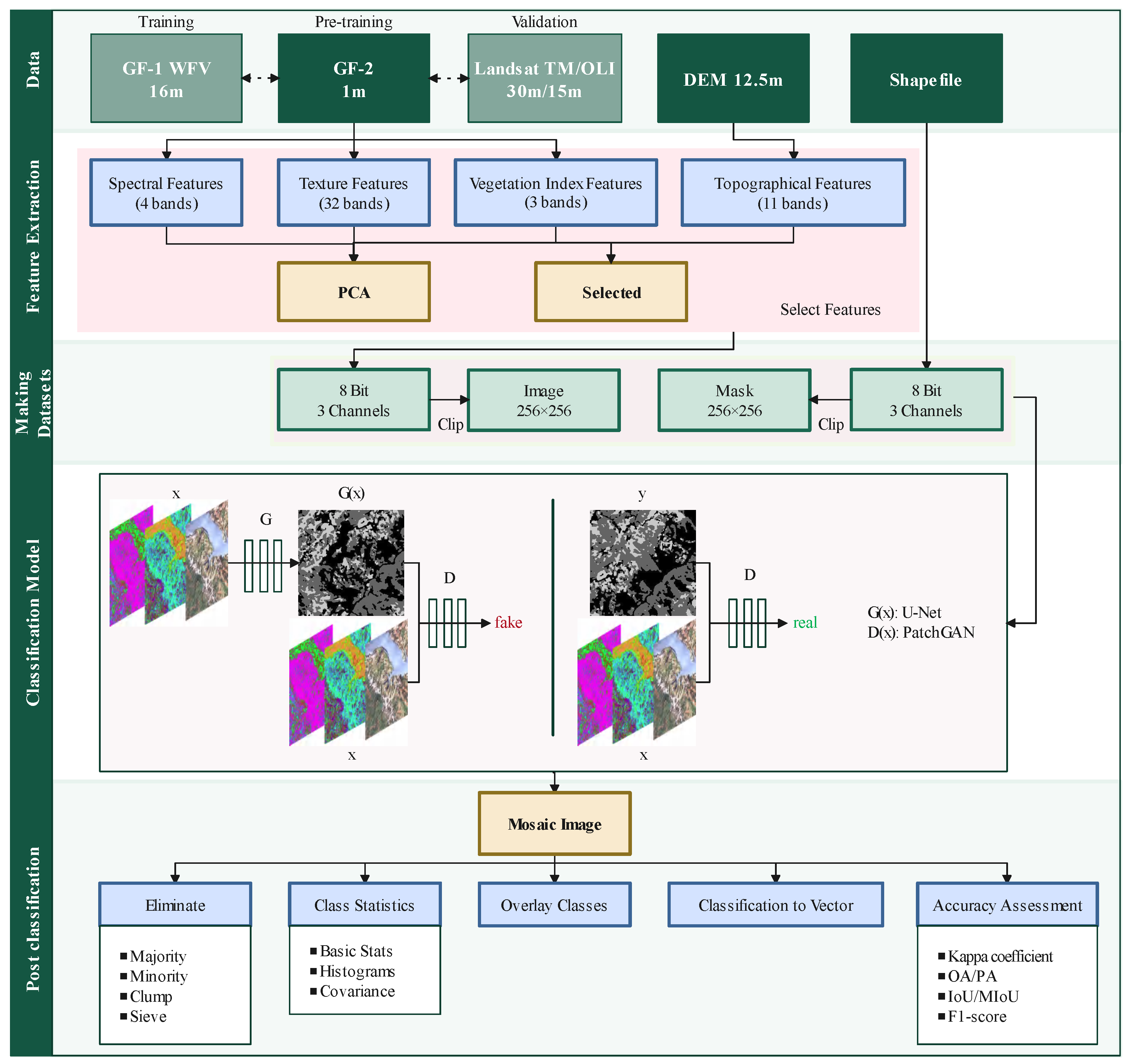
). Directly using all 50 feature descriptors was not feasible due to redundancies in feature information between needleleaf and broadleaf forest areas. Therefore, a comparison was conducted to select the most prominent feature bands to be merged and used for feature extraction in the model. The feature comparison of needleleaf and broadleaf forests is shown in Figure 2 and Figure 3, which shows that the 1st (PCA Component-1), 2nd (PCA Component-2), 18th (PCA Component-18), 82nd (GLCM Entropy-2), 83rd (GLCM Second Moment-2), and 90th (GLCM Entropy-3) feature bands were strongly distinguished, so they were combined into two sets of images for verification and comparison. Our pre-processing pipeline for the image dataset involved several steps. First, we converted the images to an 8-bit unsigned format to ensure a consistent data range. Subsequently, we synthesized the images as RGB 3-channel to enable color representation. Following that, we clipped the images to 256 × 256 size to attain uniformity in dimensions. Finally, we utilized the pre-processed dataset as a training input in Pix2Pix. The two models were the PCA-Pix2Pix model consisting of the 1st, 2nd, and 18th bands and the F-Pix2Pix model consisting of the 82nd, 83rd, and 90th bands.

2.3.3. Pix2Pix

Pix2Pix [23] was inspired from the idea of CGAN. The condition in CGAN influences the generator network and generates fake images based on the specific condition and input noise, thus performing image-to-image translation. In our image segmentation study, we used Pix2Pix’s original model structure, allowing the model to learn maximum features through the loss function in the training phase. However, we included threshold segmentation in the final layer during testing to maintain class consistency between the prediction results and labels. The structure of Pix2Pix is shown in Figure 4.

Our model employed the U-Net architecture for generator network (G) to encode and decode the input image x into a post-classification image. The role of PatchGAN, a type of conditional discriminator, in the discriminator network (D) was to assess the authenticity of G(x) and the actual post-classification image with the condition of the image x. If the generated image does not match the real image, the PatchGAN will judge it as fake.

Both the generator and discriminator used the model structure of Convolution + BatchNorm + ReLU. The loss function of the CGAN is shown in Equation (4), and Pix2Pix used $\mathcal{L}$1 regularization to make the generated images sharper, as shown in Equation (5), i.e., the $\mathcal{L}$1 distance (Manhattan distance) between the generated fake images and the real images, which ensured the similarity between the input and output images [27]. The final goal was the minimax two-player game of the generator and discriminator in the case of regular constraints. The loss function is shown in Equation (6).

$${\mathcal{L}}_{\mathrm{cGAN}}(G,D)={\mathbb{E}}_{x,y}[logD(x,y)]+{\mathbb{E}}_{x,z}[log(1-D(x,G(x,z)))]$$

(4)

$${\mathcal{L}}_{L1}\left(G\right)={\mathbb{E}}_{x,y,z}\left[\parallel y-G(x,z){\parallel }_1\right]$$

(5)

$$G^{*}=arg{min}_G{max}_D{\mathcal{L}}_{cGAN}(G,D)+\lambda {\mathcal{L}}_{L1}\left(G\right)+{\mathcal{L}}_{Focal}\left(G\right)$$

(6)

During the training process, the output image was classified by assigning each pixel to the class with the highest probability value among the 3 channels. During the prediction process, the output image was a probability map indicating the likelihood of each pixel belonging to a specific class. Each image was then arranged in a mosaic pattern. The survey statistics included area data, which were used to calculate a self-adaptive threshold. To compute the threshold, the number of pixels for each category was calculated using Equation (7). Here, $class$ represents the forest classification, $Pixels$ represents the number of pixels, $Area$ represents the corresponding area from the statistical data, and $R_{image}$ represents the spatial resolution of the satellite images, measured in meters. Next, the output images of the entire area were mosaicked, and the probability values for each classification were arranged in descending order. The $Pixels$ were chosen from this arrangement, and the minimum value among these pixels was used as the threshold. Finally, the result was generated using threshold segmentation.

$${Pixels}_{class}=Are{a}_{class}/R_{image}^2$$

(7)

2.3.4. PCA-Pix2Pix and Feature-Pix2Pix (F-Pix2Pix)

The preprocessed images underwent feature extraction using the approach detailed in Section 2.3.2. The resulting images were cropped to a size of 256 × 256 with a stride of 128. These cropped images were combined to a dataset, which served as the input for Pix2Pix, with a 6:2:2 ratio for training, validation, and testing, respectively. The GF-1 dataset comprised 1128 images, OLI had 1864 images, and GF-2 had 6205 images. However, only images with a proportion of needleleaf and broadleaf forest greater than 20% were retained from the GF-2 dataset for training and validation to ensure a balanced sample. Figure 5 displays the forest identification flow chart.

The model’s initial learning rate was set to 0.0005, and the batch size was 1. We used the Adam optimizer with linear decay [28], which occurred every 50 iterations. The dataset used for input was GF-2, and D and G models were trained alternately. The learning rate remained constant for the initial 100 epochs, followed by 300 epochs of decay. A self-adaptive threshold segmentation approach was applied, utilizing the area of needleleaf and broadleaf forests from the current year. Results were produced by applying this method to other images for identification of forest/non-forest and needleleaf/broadleaf forest, which were then arranged in a mosaic format. To mitigate the impact of a single dataset on the experimental results, we employed a five-fold cross-validation method.

The segmentation process resulted in some small spots that were removed using majority/minority analysis, clump, and sieve techniques. Based on the segmentation results, source-classified image statistics, including pixel count, minimum, maximum, and average values, and the standard deviation of each band, were calculated for each class. In the final stage, vector files were generated from these results.

The experimental configuration was Intel(R) Core(TM) i9-12900KF 3.20 GHz, NVIDIA GeForce RTX 3080Ti.

2.3.5. Accuracy Metrics

The segmentation results were examined by visually interpreting the data after adjusting the boundaries of the Third Survey data as the true values of each type. The overall accuracy (OA) [29], Kappa coefficient [30], intersection over union (IoU) [31], mean intersection over union (MIoU) [31], F1 score [32], producer accuracy (PA) [29], and user accuracy (UA) [29] were used to evaluate the accuracy of each model.

3. Results

3.1. Forest and Non-Forest Identification Results

The segmentation of forest and non-forest areas in the study area was satisfactory with the band combination of the original image for segmentation and after feature extraction, with OAs higher than 80% except for maximum likelihood (ML), as shown in

Table 3. Accuracy evaluation information of each model. Notes: the data are GF-1, and the imaging time is the summer of 2020. RF = random forest; ML = maximum likelihood; SVM = support vector machine. Bold is the best for GF-1, and underline is the second.

Dataset	Model (%)	MIoU (%)	OA (%)	Kappa (%)	Precision (%)		F1 Score (%)		IoU (%)
					Non-Forest	Forest	Non-Forest	Forest	Non-Forest	Forest
GF-1	RF	61.45	83.13	48.75	87.38	64.91	89.36	59.28	80.77	42.13
	SVM	61.41	82.29	49.37	84.82	71.45	88.60	60.43	79.53	43.29
	ML	58.54	79.05	46.03	79.02	79.22	85.95	58.87	75.36	41.71
	U-Net	76.24	88.11	72.71	87.51	89.56	91.28	81.32	83.95	68.52
	Pix2Pix	80.22	89.48	78.00	88.24	91.59	91.34	86.62	84.05	76.39
	F-U-Net	80.39	89.78	78.17	88.60	91.98	91.86	86.26	84.95	75.84
	Ours	82.93	91.25	81.26	90.28	93.05	93.06	88.17	87.02	78.85
GF-2	Ours	84.28	92.05	82.85	91.95	92.23	93.74	89.10	88.22	80.34
Landsat OLI	Ours	81.32	90.13	79.32	89.52	91.15	91.88	87.42	84.98	77.65

. The distribution of forest and non-forest was relatively balanced, but random forest (RF), support vector machine (SVM), and ML still showed low values in the IoU of the forest. Both U-Net and Pix2Pix models utilized GF-2 images as pre-training data for the segmentation process. The detailed analysis of the segmentation results, including local features, is shown in Figure 6. It should be noted that the algorithms we had chosen were universal algorithms in forest type identification. RF, SVM, and ML are algorithms in common use for remote sensing land use/land cover (LULC), while U-Net is a commonly used algorithm in deep learning semantic segmentation. Therefore, these methods have strong comparative significance.

As the most commonly used algorithm for forest segmentation, RF was chosen as the baseline for comparison purposes. ML had the lowest overall accuracy (OA), with a rate of 79.05%, approximately four percentage points lower than the baseline. The MIoU of SVM was relatively close to the baseline, whereas the OA was slightly lower than the baseline. The OA of F-Pix2Pix was 91.25%, and the MIoU was 82.93%, which were 8.12% and 21.48% higher than those of RF, respectively, with a 36.72% higher IoU in the forest. The deep learning models (U-Net and Pix2Pix) performed significantly better than the other models in all metrics. In the comparison between GF and Landsat data, both OAs were higher than 90%, the MIoU was higher than 80%, GF-1 was slightly better than OLI, and both GF-1 and OLI had decreased segmentation accuracy compared to GF-2.

3.2. Needleleaf and Broadleaf Forest Identification Results

RF, SVM, U-Net, and Pix2Pix were used to compare with the model proposed in this paper (F-Pix2Pix). The segmentation accuracy of needleleaf and broadleaf forests is shown in

Table 4. Accuracy evaluation information of each model. Notes: the data are GF-1, and the imaging time is the summer of 2020. RF = random forest; ML = maximum likelihood; SVM = support vector machine. Bold is the best for GF-1, and underline is the second.

Dataset	Model	MIoU (%)	OA (%)	Kappa (%)	Precision (%)			IoU (%)
					Other	Needleleaf	Broadleaf	Other	Needleleaf	Broadleaf
GF-1	RF	42.57	77.59	36.92	86.13	44.10	25.65	79.52	31.75	16.43
	SVM	42.12	75.13	36.21	82.15	47.74	31.72	77.15	32.68	16.51
	ML	39.82	68.06	31.69	73.22	46.04	45.68	70.82	33.07	15.57
	U-Net	41.44	71.65	33.45	79.23	65.55	18.06	61.97	51.77	10.58
	Pix2Pix	40.88	70.95	34.21	81.22	61.39	21.85	62.39	49.76	10.48
	PCA-RF	44.56	79.09	40.16	87.38	46.82	27.61	80.77	35.97	16.94
	PCA-SVM	45.74	78.22	41.69	84.82	52.90	35.40	79.53	39.85	17.85
	PCA-ML	43.50	73.25	36.81	79.02	48.70	47.78	75.36	38.06	17.07
	PCA-U-Net	63.02	78.57	60.43	78.65	88.37	37.19	68.07	78.24	22.29
	PCA-Pix2Pix	69.13	80.46	66.42	79.34	88.52	59.53	68.97	78.49	41.61
	F-U-Net	69.13	83.65	73.98	78.37	92.37	67.04	69.85	76.63	60.92
	Ours	72.01	84.85	75.87	78.35	88.22	82.99	71.73	77.36	66.93
GF-2	Ours	77.43	87.22	80.34	87.47	89.83	83.77	80.16	80.70	71.44
Landsat OLI	Ours	72.18	84.18	75.27	84.40	88.52	77.29	75.80	78.49	62.26

. In all experiments, the accuracy of using only the original spectral information was the lowest. However, the OA was still higher than 65%, comparable to that of existing product data. Nonetheless, a significant class imbalance persisted, resulting in an IoU of less than 20% for broadleaf forest, rendering it unrecognizable. RF, SVM, and ML had comparable performance effects with the deep learning models of U-Net and Pix2Pix, all of which were more affected by the class imbalance, and even the IoU of broadleaf forest was still significantly lower than that of the three machine learning models, with U-Net performing slightly better than Pix2Pix. Regarding the segmentation of images after PCA feature extraction, U-Net and Pix2Pix were significantly better than the remaining three models (RF, SVM, and ML), which showed the advantage of the transfer-learning-based domain adaptation method of multi-source image for semantic segmentation. Although the advantages appeared, they were still not significant, the IoU of broadleaf forest was still significantly lower than others, and the accuracy of Pix2Pix for broadleaf forest identification was higher than U-Net. Overall, the identification of needleleaf forest was better than broadleaf forest, and the local features of the results are shown in Figure 7.

The accuracy values of needleleaf and broadleaf forest were effectively improved, but the accuracy of Other was lost. However, we utilized vegetation index and high-accuracy forest/non-forest segmentation results to filter the segmentation in the application, resulting in enhanced utility of the results.

The F-Pix2Pix results with the highest accuracy were used to calculate the area of needleleaf and broadleaf forests. The area of needleleaf forests in the study area was 2612.92 km${}^2$, and the area of broadleaf forests was 228.90 km${}^2$. The needleleaf forests in the forest management inventory data were 2376.35 km${}^2$, and the broadleaf forests were 256.44 km${}^2$, with relative errors of 7.73% and 10.16%, and the mean relative error was 8.94%. With prior knowledge, adding prior statistics using the self-adaptive thresholding segmentation method can maximize the number of pixels required for each class and effectively improve the segmentation accuracy.

The results presented above were obtained using GF-1 imagery. We also evaluated other datasets imaged during the summer of 2020, including GF-2 and Landsat OLI, utilizing the proposed model (F-Pix2Pix). The segmentation accuracies of the three datasets were similar, accurately identifying both needleleaf and broadleaf forests and effectively avoiding class imbalance. Specifically, GF-2 had the highest accuracy and the greatest differentiation between needleleaf and broadleaf forests, which might be attributed to superior resolution. Further investigation was required to determine the exact extent of its impact. These results demonstrated that the proposed model performed well on various datasets, achieved cross-scale segmentation, and exhibited strong generalizability.

3.3. Spatial and Temporal Characteristics

The spatial distribution of forest types from 2005 to 2020 is shown in Figure 8, where (a) is forest/non-forest and (b) is needleleaf/broadleaf forest. The forest type changes information is shown in

Table 5. State transition of forest types from 2005 to 2020. Note: the calculation method for forest state change is the difference between the identification results in 2005 and 2020.

Type	States	Total Pixels	Area (km2)	Ratio (%)
Forest/Non-forest	Forest→Non-forest	4096	468.94	7.97
	Non-forest→Forest	5714	654.19	11.12
	Non-forest unchanged	20,403	2335.91	39.72
	Forest unchanged	21,149	2421.32	41.18
Needleleaf/Broadleaf	Broadleaf→Other	431	49.34	0.84
	Broadleaf→Needleleaf	577	66.06	1.12
	Broadleaf unchanged	533	61.02	1.04
	Needleleaf→Other	3279	375.41	6.37
	Needleleaf→Broadleaf	439	50.26	0.85
	Needleleaf unchanged	16,665	1907.95	32.40
	Other→Broadleaf	1247	142.77	2.42
	Other→Needleleaf	3567	408.38	6.93
	Other unchanged	24,705	2828.44	48.02

. The forest cover ratio in 2020 is 52.30%, which is 12.4% higher than that in 2005. During the evolution of forest types from 2005 to 2020, 11.12% of non-forest was converted to forest, while 7.97% changed from forest to non-forest. The area with unchanged forest and non-forest was 4757.23 km${}^2$, accounting for 80.9%, of which 2421.32 km${}^2$ (41.18%) was unchanged by forest. Analysis of spatial distribution characteristics indicated that the areas where non-forests converted to forests were scattered throughout the study area. Conversely, the areas where forests transformed into non-forests were concentrated and primarily located in the northern, central, and southwestern parts of Huize County.

The change in the type of needleleaf and broadleaf forest contains nine statuses. In the past 15 years, the area with no change in type is 4797.41 km${}^2$ (81.46%). The proportion of needleleaf forests was 32.40%, which was 31.15 times higher than that of broadleaf forests. Other to needleleaf and broadleaf forest is 551.15 km${}^2$ (9.35%), of which needleleaf forest is 6.93%, which is 2.86 times more than that of broadleaf forest. During the evolution, 424.75 km${}^2$ of needleleaf and broadleaf forests were converted to Other, accounting for 7.21%, and the needleleaf forests were 7.61 times more than the broadleaf forests. The area of needleleaf and broadleaf forest interconversion is 116.32 km${}^2$, accounting for 1.97%, and they are relatively close. Among all the statuses with alteration, the largest area of conversion between needleleaf forest and Other was 783.79 km${}^2$, with a total of 13.30%. Among the spatial distribution characteristics, the conversion of Other to needleleaf forest was mainly distributed in the north, central, and south, while the conversion of needleleaf forest to Other was mainly distributed in the west and central, and the rest of the statuses were relatively scattered.

4. Discussion

4.1. Comparison of Segmentation Methods

4.1.1. Feature Extraction

With PCA for multi-feature dimensionality reduction, this process may lose the most useful information for this task [33], and the PCA transform does not target better retention of data information when the data detail is completely unknown. Decentralization and standardization are needed in data pre-processing, especially for data contaminated by noise, where the standard deviation of the noise amplifies the data more significantly, while data not contaminated by noise amplify less in the process of standardization, resulting in unsatisfactory segmentation results after feature extraction. It is simple and feasible to directly select the feature combinations that have obvious differences between needleleaf and broadleaf forest areas for segmentation.

In semantic image segmentation tasks, deep learning models have higher accuracy than other models [17,34,35]. However, for simple tasks, the advantages of deep learning have not been manifested, such as for the identification of forests and non-forests. Although the segmentation accuracy of the deep learning model is still slightly higher than that of other models, neither the system overhead nor the running process is advantageous. For complex tasks such as needleleaf and broadleaf forest identification, the advantages of deep learning models can be demonstrated, but the optimization of their performance still needs to be explored in depth.

Forest types are highly correlated with topographic features [36,37], and single-temporal images combined with topographic features can effectively be identified [38,39]. However, the terrain of the study area is complex, with a large range in elevation (695∼4017 m). The experiments show that adding topographic features does not effectively distinguish between needleleaf and broadleaf forests, and this method is not effective in this study area.

4.1.2. Class Imbalance

The needleleaf and broadleaf forests in the study area are unevenly distributed, the broadleaf forests account for a relatively small proportion of the total, and there is a serious class imbalance problem. Class imbalance, also called data skew and data imbalance, refers to the situation in which the number of training samples of different classes in the segmentation task varies greatly. To address this problem, we focus the training sample range on the region with a relatively uniform distribution of needleleaf and broadleaf forests. Furthermore, Pix2Pix outperforms U-Net in class imbalance for segmentation, which reflects the advantage of image-to-image semantic segmentation. It may be that the Pix2Pix algorithm is mostly used for image translation, and the grasp of details is better than that of segmentation methods such as U-Net. When class imbalance is not considered, the intersection over union (IoU) of the broadleaf forest in each algorithm is lower than 30%. After solving the class imbalance problem with the transfer learning domain adaptation method, the OA of U-Net substantially advanced from 71.65% to 83.65%, indicating a 12% enhancement. Furthermore, the IoU of the broadleaf forest escalated from 10.58% to 60.92%, denoting a remarkable improvement of approximately 50.34%. Similarly, the OA of Pix2Pix accelerated from 70.95% to 84.85%, and its associated IoU augmented from 10.48% to 66.93%, signifying a significant boost of 56.45%.

4.1.3. Cross-Resolution

In this study, we approached remote sensing semantic segmentation by converting a pixel classification challenge into an image translation task. The focus of the model training was mainly on a pixel level, where the original full-view image was cropped to a size of 256 × 256. Our experimental results show that different resolution images are used for forest identification, and long time series forest identification and monitoring can be performed by multi-source images, but the effect of data distribution differences on semantic segmentation needs further in-depth study in the future.

4.2. Comparison of Products

Three products, FROM-GLC-seg, Forest2010, and ESA GlobCover, were selected for comparison with our results, and the validation accuracy is shown in

Table 6. Comparison of product accuracy. Notes: ours refers to the F-Pix2Pix model. The comparative area is the study area, namely Huize County, Qujing City, Yunnan Province, China. The remote sensing image is Landsat TM data, and the imaging time is 2010. Bold is the best, and underline is the second. Our data are generated from the trained model of Landsat OLI images in 2020.

Type	Product	Kappa (%)	OA (%)	PA (%)	UA (%)
Forest/Non-Forest	Ours	77.43	87.84	84.80	80.95
	FROM-GLC-seg	52.51	84.56	77.61	75.12
	Forest 2010	28.35	82.16	82.93	60.39
	ESA GlobCover	35.80	80.67	71.33	65.85
Needle/Broadleaf Forest	Ours	70.55	83.27	70.03	69.63
	FROM-GLC-seg	49.10	83.02	55.61	54.29
	Forest 2010	28.03	81.99	57.79	40.76
	ESA GlobCover	32.68	79.44	47.01	43.66

. FROM-GLC-seg [40] and Forest2010 [41] are needleleaf and broadleaf forest products for 2010, and the method is RF with a spatial resolution of 30 m. Forest2010 is the product for China, and OA is 72.7%. ESA GlobCover2009_V2.3_Global is a 2009 product with the RF method and a spatial resolution of 300 m [42]. All three products cover Huize County (the study area of this paper), and Landsat TM 2010 images were selected for comparison. The validation data are from the forest management inventory.

In forest and non-forest identification, the differences in OA, PA, and UA of each product are relatively small, but the differences in Kappa coefficients are large, indicating that the consistency effect of product spatial distribution is poor. In the identification of needleleaf and broadleaf forests, OA is close, but the differences between the remaining three metrics are obvious, which is still mainly due to the lower identification of broadleaf forest in the case of class imbalance. The proposed method outperforms the existing products in various evaluation metrics, with better generalization capabilities. These findings imply that the proposed model can effectively identify the forest types in a large area.

5. Conclusions

The study area was located in Huize County, Qujing City, Yunnan Province, China. We utilized the GF and Landsat satellite images as data and proposed the F-Pix2Pix semantic segmentation method employing the concept of deep learning image translation. The identification of forest/non-forest and needleleaf/broadleaf forest provided a foundation for the accurate estimation of regional carbon sinks. The main conclusions were as follows:

• The F-Pix2Pix proposed in this paper had the best results, with higher accuracy than the existing products, 21.48% in non-forest/forest and 29.44% in needleleaf/broadleaf forest, for MIoU improvement. The distinction between forests/non-forests is higher than that between needleleaf and broadleaf forests. In future applications, the former can provide support for the latter to improve identification accuracy.
• Applying transfer learning domain adaptation to semantic segmentation showed significant benefits, and this approach yielded better results for needleleaf/broadleaf forests in comparison to forest/non-forest. Furthermore, this method utilized satellite images of different resolutions to solve the class imbalance problem.
• We implemented semantic segmentation by image-to-image translation, and the F-Pix2Pix not only effectively solved the class imbalance but also demonstrated good performance in different satellite images. It can be used for multi-source images with strong generalization, which provides the possibility of long-term monitoring. The identification of needleleaf and broadleaf forests combined with the actual geographical characteristics of the forest was the basic work for the accurate estimation of regional carbon sources/sinks.