Abstract
High-resolution multispectral remote sensing images offer valuable information about various land features, providing essential details and spatially accurate representations. In the complex urban environment, classification accuracy is not often adequate using the complete original multispectral bands for practical applications. To improve the classification accuracy of multispectral images, band reduction techniques are used, which can be categorized into feature extraction and feature selection techniques. The present study examined the use of multispectral satellite bands, spectral indices (including Normalized Difference Built-up Index, Normalized Difference Vegetation Index, and Normalized Difference Water Index) for feature extraction, and the principal component analysis technique for feature selection. These methods were analyzed both independently and in combination for the classification of multiple land use and land cover features. The classification was performed for Landsat 9 and Sentinel-2 satellite images in Delhi, India, using six machine learning techniques: Classification and Regression Tree, Minimum Distance, Naive Bayes, Random Forest, Gradient Tree Boosting, and Support Vector Machine on Google Earth Engine platform. The performance of the classifiers was evaluated quantitatively and qualitatively to analyze the classification results with whole image (comprehensive feature) and small subset (targeted feature). The RF and GTB classifiers were found to outperform all others in the quantitative analysis of all input combinations for both Landsat 9 and Sentinel-2 datasets. RF achieved a classification total accuracy of 96.19% for Landsat and 96.95% for Sentinel-2, whereas GTB achieved 91.62% for Landsat and 92.89% for Sentinel-2 in all band combinations. Furthermore, the RF classifier achieved the highest F1 score of 0.97 in both the Landsat and Sentinel datasets. The qualitative analysis revealed that the PCA bands were particularly useful to classifiers in distinguishing even the slightest differences among the feature class. The findings contribute to the understanding of feature extraction and selection techniques for land use and land cover classification, offering insights into their effectiveness in different scenarios.
1. Introduction
Land Use Land Cover (LULC) change is one of the most important drivers of global change, affecting many aspects of the natural ecosystem and environment such as biodiversity, water, soil quality, and the radiation budget [1,2]. LULC change detection aids policymakers in comprehending the dynamics of environmental change to assure long-term growth. As a result, LULC feature identification has become an essential research topic, necessitating the development of a reliable LULC classification system. The enumeration of spatiotemporal LULC dynamics has become straightforward, quick, cost-effective, and accurate because of the emergence and development of integrated geospatial approaches that combine remote sensing (RS) and geographic information systems (GIS).
The image classification approach can be broadly categorized into unsupervised, supervised, and object-based classification [3]. The selection of the classification approach depends on the study objectives, the complexity of the scene, the availability of training data, and the desired level of detail in the classification results. The supervised classification technique is the most widely used; however, object-based classification has proved to be more conceivable for high-resolution satellite and unmanned aerial vehicle (UAV) images for visible-range LULC features [4,5,6,7]. When dealing with spectrum mixes, a hybrid classification technique is frequently employed to separate object characteristics. On the other hand, the use of multi-source data or multi-indices data can increase classification accuracy [8,9]. Researchers have developed several spectral indices based on image band statistics, such as the Normalized Difference Built-up Index (NDBI) [10,11], Normalized Difference Vegetation Index (NDVI) [12,13,14], Normalized Difference Water Index (NDWI) [15,16], Enhanced Night-time Light Urban Index [17], Compounded Night Light Index [17], etc., to extract LULC features [18,19,20,21]. Spectral indices offer numerous benefits, but they can only be used for extracting primary LULC features and, their classification accuracy is limited because of their dependency on selected bands and linear analytics. Researchers often used principal component analysis (PCA), a statistical approach for reducing the dimension of multispectral satellite imagery and minimizing the correlation between feature classes and bands [22,23]. The key advantages of using PCA for classification are the independent and uncorrelated information of features in PC bands, which enable more accurate separation of natural and artificial features.
In the last two decades, with the advent of artificial intelligence (AI) as an analytical approach, advanced methods for LULC classification have garnered attention, such as Artificial Neural Networks (ANN), Support Vector Machine (SVM), Random Forest (RF), Fuzzy Adaptive Resonance Theory-supervised Predictive Mapping (Fuzzy ARTMAP), Classification And Regression Tree (CART), Minimum Distance (MD), Naive Bayes (NB), Decision Tree, Gradient Boosted Trees (GBT), and other models [20,24,25,26,27]. RF is a nonparametric machine learning-based classification algorithm that uses ensembles of decision trees to achieve the best classification accuracy [28,29,30,31]. SVM produces the hyperplane in the N-dimension, to detect possible separability between the class for the classification [28,29,30,31]. Based on nonparametric decision trees, CARTs create binary trees for the collected samples and use them for classification [32,33,34,35]. NB works on Bayesian theory for classification. It is a probabilistic machine learning classifier, which uses the decision tree for structuring and organizing the generated probability-based NB model [36,37,38]. MD takes the spectral values of the center of the cluster in the training data to calculate the value of the unknown class, based on the distance between the center of the cluster and the unknown class [39,40,41,42]. GTB is an ensemble model made up of many CART algorithm implementations. Following the construction of the initial tree, GBM constructs subsequent trees by adjusting the weights of input data and achieving higher prediction accuracy.
Previous studies have explored the benefits of using spectral bands, indices, and PCA either individually or in limited combinations with various classifiers, focusing primarily on overall accuracy assessment. However, there is a research gap when it comes to analyzing classifier performance for individual classes in whole image. In this study, our objective was to address this gap by thoroughly examining the performance of different machine learning classifiers using multiple input combinations. We conducted a comprehensive analysis of classifier accuracy at both comprehensive feature and targeted feature, allowing for a detailed assessment of their performance across larger areas and smaller subsets. Our analysis included the utilization of multispectral satellite bands, spectral indices, and PCA applied to the multispectral bands, both individually and in combination, for accurate land use and land cover feature classification. The classification was performed for Landsat 9 and Sentinal-2 satellite images in Delhi, India, using six machine learning techniques—CART, MD, NB, RF, GTB, and SVM—on Google Earth Engine (GEE). These classifiers have been extensively researched and widely used in land cover classification studies, particularly when considering the entire image. However, there is a research gap when it comes to evaluating the performance of these classifiers specifically for individual feature classes within the entire study region. The GEE is a geospatial processing platform that provides an effective infrastructure for large-scale processing with inbuilt support for ML algorithms. Earlier studies have shown that ML classification techniques achieve better overall accuracy in comparison to conventional statistical techniques. To thoroughly investigate the classification capabilities of the used classifier, we have compared the performance of the classifiers on various land cover classes. Although overall classification accuracy is an important metric, it is equally important to evaluate the performance of each classifier across different classes. Surface feature extraction from classified images is a crucial task in many applications, and the accuracy of specific classes of interest can greatly impact the reliability of the extracted information. Some machine learning algorithms may demonstrate high overall accuracy but perform poorly when it comes to specific classes. Therefore, a comprehensive analysis of classifier performance across different classes is essential to assess their suitability for specific applications and to ensure accurate feature extraction for further studies.
2. Study Area
We have chosen an area for the study that has diversified urban formations and feature classes. The study area includes the National Capital Territory (NCT) of Delhi, as well as nearby suburbs and satellite cities such as Dadri, Gurugram, Faridabad, Ghaziabad, and Meerut. The location map of the study area with specifically selected urban and nonurban subsets (classes) is presented in Figure 1.
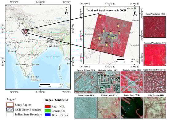
Figure 1.
The location map of the study region with examples of urban and nonurban subsets from Sentinel-2 images in false colors, as reported in the legend.
The study area is spread over 8602.62 square kilometers and is located between latitudes 28.155N and 29.256N and longitudes 76.83E and 77.895E. It contains a variety of natural landforms, including a central ridge reserve forest, numerous tiny hills, three major rivers, and several small lakes. Since this region started urbanizing several decades before and continues to accelerate in recent years, we could see numerous urban formations, ranging from dense to sparse, formal to informal, horizontal to vertical, etc.
3. Data Used
Data at the resolution of 10 m/pixel to 30 m/pixel were more suited for LULC [27,43,44,45]. The analysis was conducted using the most recent satellite dataset from Sentinel-2 and Landsat 9 mid-resolution satellites, archived on GEE. The datasets were corrected for atmospheric effects and orthogonally aligned using the Landsat Ecosystem Disturbance Adaptive Processing System (LEDAPS) algorithm [46]. The study area was covered in multiple images that are represented by path and row or tile number, given in Table 1. Each tile was filtered with a cloud cover of less than 10%, and the images with the least cloudiness were chosen for analysis.

Table 1.
Details of satellite images used in the study.
For the analysis, Landsat data with an original spatial resolution of 30 m and Sentinel data with bands at 20 m resolution that were rescaled to 10 m were used. The total number of pixels used for the study was 860 × 106 for Sentinel data and 286 × 106 for Landsat data. Out of these pixels, approximately 1130 samples were selected across all classes for training and testing the algorithm. To ensure an effective evaluation of the classifiers, a random sampling approach was employed. The selected samples were divided into two sets: 70% of the samples were used for training the classifiers, and the remaining 30% were used for testing and evaluating the classifier’s performance. It is important to note that a very high-resolution image was used as the ground truth reference data for collecting the training and testing samples. This high-resolution image provides more detailed and accurate information about the land cover classes, allowing for precise identification and sampling of the desired features. The selection of samples for each class took into consideration various image interpretation factors such as spectral reflectance, texture, shape, and contextual information to ensure a representative and diverse dataset. For both Landsat and Sentinel data, the training and testing samples were selected at the same spatial locations. The classification process was conducted separately for Landsat and Sentinel data, treating them as individual datasets. This approach allowed for independent evaluation and comparison of the classifiers’ performance using Landsat and Sentinel imagery.
4. Methodology
A flow chart diagram describing the methodology is presented in Figure 2. To run the classification algorithms, satellite images are pre-processed after being retrieved from the GEE archive. To select the input variables for classifications, all the multispectral bands that contain the most information regarding targeted features were filtered, and the spectral indices and the PCA math bands were generated. In the second step, multiple machine learning algorithms were employed to classify different combinations of predictors as inputs. The third step involved analyzing the performance of each classifier by assessing the classification results for both comprehensive feature and targeted feature using quantitative and qualitative evaluation techniques, respectively. Finally, the results obtained from this analysis allowed the identification of the optimal classifier and predictor combination for accurately classifying surface features.
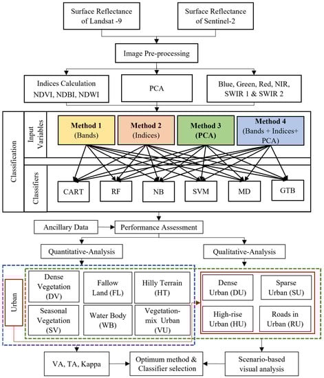
Figure 2.
Complete flow chart of the proposed methodology. In the quantitative analysis, the entire region was assessed with seven land cover classes (comprehensive feature, blue dashed box, cfr. Section 5.1), whereas in the qualitative analysis, subsets were selected for each of the ten classes (targeted feature, green dashed box, cfr. Section 5.2).
4.1. Input Selection
Machine learning has the potential to enhance remote sensing image classification by effectively handling high-dimensional data and mapping classes with complex properties [28,47,47]. Although incorporating more predictor variables can provide additional information to differentiate between classes, it can also lead to a decrease in classification performance due to the curse of dimensionality or the Hughes phenomenon. Therefore, when using machine learning classifiers, selecting the appropriate input variables is crucial to eliminate the curse of dimensionality and save computational resources [47]. To determine the optimal input variable combination for classification, we experimented with various combinations listed in Table 2.
Table 2.
List of the four different input combinations (referred to as “method,” as in Figure 2) used for classification. PC-1, PC-2, and PC-3 are the first three PCA components (see Section 4.1.3).
4.1.1. Band Optimization
Generally, LULC classification is performed with all multispectral bands in machine learning models, as they contain some part of the information about the various land surface features. Landsat 9 has nine multispectral bands, of which band 8 is a panchromatic band with a spatial resolution of 15 m, and bands 1 and 9 have high atmospheric absorption; hence, in the current study, bands 2 to 7 were chosen for LULC classification. Sentinel-2 satellite comprises 13 multispectral bands with varying spatial resolutions in the range of 10 m to 60 m. To compare the classification accuracy of Landsat 9 and Sentinel-2 satellites, we selected the corresponding Sentinel bands that match the selected Landsat bands. This includes bands 2 to 4, as well as bands 8, 11, and 12, which were chosen for the analysis. Figure 3 highlights the advantages of using the spectral reflectance values from the selected bands in distinguishing between different urban and nonurban land cover features. The variation in surface reflectance values for each class demonstrates the potential of using these spectral characteristics for accurate classification.
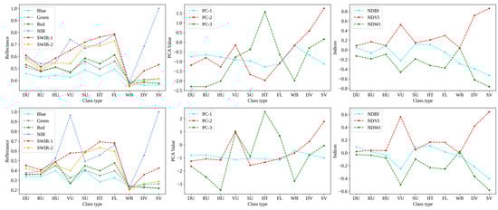
Figure 3.
Spectral reflectance (first column), PCA values (second column), and spectral indices (third column) for the different urban and nonurban classes by using Landsat (first row) and Sentinel-2 (second row) data. A polygon of the same size was drawn for each class and the average of the pixel values within each class’s polygon was computed.
4.1.2. Spectral Indices Calculation
The combination of reflectance spectra from multiple wavelengths can be used to create spectral indices that facilitate the estimation of the relative abundance of specific features of interest. Our research area is characterized by a high proportion of buildings, vegetation, and water bodies. Therefore, we used spectral indices such as NDBI to extract building information, NDVI [12,13,14,15,16] to extract vegetation information, and NDWI to extract water body information. These indices were used to generate index-based inputs for classification purposes, as presented in Table 3. Figure 4 displays the results of applying NDBI, NDVI, and NDWI on Landsat 9 and Sentinel-2 images.
Table 3.
Summary of the spectral indices used as input for classification.
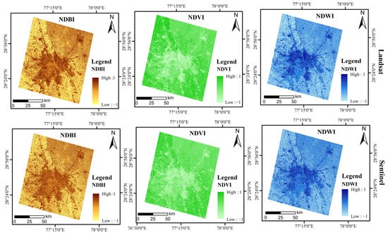
Figure 4.
NDBI, NDVI, and NDWI were derived over the study area from the Landsat and Sentinel images.
4.1.3. Principal Component Analysis
The PCA is the most extensively used technique for reducing dimensions and selecting features from multidimensional datasets [22,23,53]. It extracts relevant data and compresses data without losing much of the original information. In PCA, the image bands are changed into new bands known as primary or principal components, which are then arranged in decreasing order by how much image variance they can represent. The most informative six satellite bands chosen from Landsat (bands 2 to 7) and Sentinel images (bands 2 to 4, bands 8, 11, and 12,) through the band optimization technique described in Section 4.1.1 were fed into PCA, and six principal components resulted from the analysis. The most comprehensive components PC-1, PC-2, and PC-3 were provided as input to the machine learning classifiers.
4.2. LULC Classification Using Machine Learning
The cloud-based tool Google Earth Engine allows scientists to analyze and visualize geospatial datasets and images dating back several decades. GEE’s classifier package supports supervised classification with traditional machine learning algorithms [54,55,56]. The classification algorithms used for the study are NB, CART, RF, GTB, and SVM. Hyperparameters for these algorithms are determined empirically by systematically searching through a range of values to find the optimal settings that maximize performance for the specific dataset. A brief discussion of the individual classifier is as follows:
SVM was developed by Vapnik in 1995 and was derived from statistical learning theory [57]. The SVM is a nonparametric supervised classification system that uses a hyperplane to achieve the ideal border that minimizes the separation, or margin, between the support vectors [28,29,30,31]. As it offers the advantage of dividing between vectors, SVM was commonly employed to separate the distinct classes in LULC classification [27]. GEE supports the SVM algorithm for classification, which is defined by parameters such as kernel type, cost, and gamma. The choice of kernel type has a significant impact on the classification results. For the analysis, the relatively stable RBF (Radial Basis Function) kernel function was chosen. Additionally, the gamma and cost parameters are important in determining the performance of the SVM classifier. These parameters control the complexity of the decision boundary and the penalty for misclassification. The values of gamma and cost were selected through experimental trial-and-error methods.
The Minimum Distance method was proposed by J. Wolfowitz in 1953 [58]. MD categorizes the measurement vectors into groups rather than individual vectors. This conventional pixel-based classification strategy uses the distance between unknown classes and the cluster’s center for the classification [40,41,42]. In GEE, the algorithm calculates the Euclidean distances based on the feature vectors of the training samples without the need for parameter tuning.
The Bayes theorem served as the basis for the formulation of the NB. The Bayesian theory is a method of calculating the chance of another event occurring based on the probability of a previous event [36,37,38]. NB machine learning classifier builds a probability-based model with strong (naive) assumptions of independence between features. The NB classifier in GEE uses a probabilistic approach that assumes feature independence to classify data. It calculates the probabilities of a sample belonging to each class based on the feature values, enabling the classification process.
The CART method was first proposed in 1984 based on the Bayesian model [59]. The CART is a nonparametric classification algorithm that constructs a binary tree from a remotely sensed sample by splitting the parent node into two child nodes and treating each child node as a prospective parent node for further splitting using Gini’s impurity index. It has been widely used for the classification of impervious surfaces [32,34,60,61].
In 1995, Tin Kam Ho used the random subspace approach to construct the first algorithm for random decision forests algorithm. The RF is a strong ensemble machine learning classifier that uses K binary CART trees to classify data. Each tree is created by running a separate learning algorithm that divides the input variable collection into subgroups based on attribute values [62,63,64,65].
Breiman put forth the concept of gradient boosting in the late 19th century, saying that it might be thought of as an optimization technique based on an appropriate cost function [62]. GTB techniques use a collection of decision trees, similar to RF [66,67]. However, the underlying technique differs in that it limits the complexity of trees and constrains each tree to a weak predictive model. It uses a gradient descent approach to iteratively transform an ensemble of these weak learners into strong ones by minimizing a differentiable loss function at each step to achieve classification accuracy [68,69,70].
In decision tree-based classifiers the hyperparameters can be adjusted to control the complexity of the model and find the right balance between simplicity and accuracy. Parameters such as maximum tree depth, minimum samples per leaf, or the number of trees in a random forest can be tuned based on the characteristics of the dataset and the desired model performance. In the case of constructing a decision tree, determining the optimal number of nodes and branches is crucial. For the study, the leaf population parameter is defined within the range of 0 to 10, which specifies the maximum number of data points allowed in a leaf node. However, the number of nodes parameter is not pre-defined in GEE, allowing for an unlimited number of nodes to be created in the tree. This flexibility allows the algorithm to adapt and optimize the construction of the decision tree based on the specific dataset and classification requirements.
Furthermore, a fixed number of training and testing samples were used for all the classifiers in the study. This consistent approach ensures fairness and enables a reliable comparison of the performance of the different algorithms.
4.3. Class and Site Selection for Targeted Feature Analysis
The purpose of LULC classification is to extract specific land cover features of interest from remotely sensed images, but not all surface features are relevant. To overcome the difficulty of binarily classifying all surface features, we selected seven classes for classification, namely urban, vegetation-mix urban (VU), dense vegetation (DV), seasonal vegetation (SV), water body (WB), fallow land (FL), and hilly terrain (HT). The performance of the classifiers was evaluated quantitatively at the comprehensive class (the entire study area of Figure 1) for these seven classes.
However, machine learning classifiers tend to weigh all classes equally, which may lead to misclassification of the class of interest. Analyzing the accuracy of specific classes becomes challenging due to the complex terrain and mixed pixel compositions. To overcome this challenge, we carefully selected a small subset of pixels for each class that was both dominant and representative of the class. This subset allowed us to assess the effectiveness of the classifier at a targeted feature, focusing on five urban and five nonurban regions that represented different classes. Although there could be many subcategories among the seven classes, it can be difficult to differentiate them in coarser-resolution images due to complex textures. Therefore, we further divided the urban class into dense urban (DU), sparse urban (SU), high-rise urban (HU), and roads in urban (RU) because the urban class exhibits apparent differences in texture and spectral reflectance based on urban formations. HU is a 3D characteristic derived from 2D satellite images based on specific criteria. Urban areas often have a distinctive skyline dominated by tall buildings. In the analysis of high-resolution satellite imagery, we identify clusters of buildings with similar heights or patterns as indicators of a high-rise urban environment. Additionally, during daylight hours, these buildings can cast shadows, appearing as dark shades in satellite images. It is important to note that distinguishing between water and shadows can be challenging as they may exhibit similar reflectance in the images. However, examining the surrounding objects can aid in differentiating between these features. A total of 10 classes were selected, and for each class, we chose a subset of equal area (1.28 km2) to analyze the machine learning classifier’s performance across different land cover types.
5. Results
5.1. Quantitative Performance Evaluation of Machine Learning Classifiers at Comprehensive Class
Classification accuracy is a measure of the difference between the acquired geographic phenomena and the classified map [45,61]. To evaluate the accuracy of the generated land cover maps, very high-resolution images were used as reference data. Various evaluation measures, including the confusion matrix, validation overall accuracy (VA), training overall accuracy (TA), the kappa statistic, and the F1 score, were employed [55,62]. The relationship between classification accuracy and the kappa coefficient is given in [34]
The kappa coefficient, denoted by K, is a measure of classification accuracy. It is calculated using a confusion matrix, which consists of the n number of classifications for each land cover class. Kii represents the number of pixels that are correctly classified for class i, whereas Ki+ and K+j are the total number of pixels in the ith row and jth column, respectively. T represents the total number of pixels used for evaluating the accuracy [63,64].
In the land-use and landcover classification, the RF classifier outperformed other classifiers by using method 1 as input (i.e., using satellite bands alone), achieving the highest training accuracy (TA), 96.70% and 97.21%, and the highest kappa, 95.93% and 96.55%, for Landsat and Sentinel images, respectively. Additionally, the RF classifier achieved the highest F1 score of 0.97, indicating a balance between precision and recall in accurately classifying the land cover features in both datasets. RF classifier results, for both Landsat 9 and Sentinel-2 images, are presented in Figure 5. Following the RF classifier, the GTB classifier had the next highest F1 score of 0.92, suggesting its effectiveness in the classification task. Gradient Boosting (GTB) classifier also produced high accuracy with method 4 as input, i.e., combining sensor bands with additional information from indices and PCA, yielding a high validation overall accuracy (VA) of 83.53% and 80.59% for Landsat and Sentinel images, respectively. Additionally, RF classifier produced the highest VA of 80.59% for the Sentinel image in method 4. Figure 6 shows the classification accuracy of the various classifiers using the four different input methods for the Landsat 9 image, and Figure 7 the same for the Sentinel-2 image.
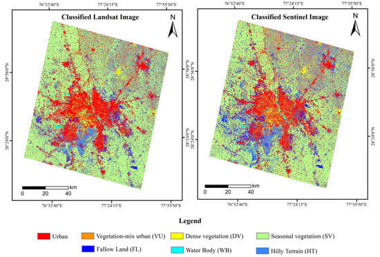
Figure 5.
Comprehensive class analysis: Landsat 9 and Sentinel-2 images of the entire region were classified using the RF classifier with 7 LULC classes.
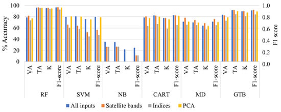
Figure 6.
Evaluation of Landsat 9 image classification accuracy (VA, TA, K, and F1 score) using various classifiers (RF, SVM, NB, CART, MD, GTB) with the four input methods.
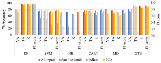
Figure 7.
Evaluating the classification accuracy of Sentinel-2 image (VA, TA, K, and F1 score) using various classifiers (RF, SVM, NB, CART, MD, GTB) with the four input methods.
The Naive Bayes classifier produced the lowest accuracy compared to the other classifiers, as it relies on the probability of past events and any errors propagating forward. method 2, which only used spectral indices, resulted in the lowest accuracy when classified with all the selected machine learning classifiers. However, adding spectral indices and PCA to the Landsat satellite bands (method 4) increased the accuracy of the SVM and NB classifications, and adding them to the sentinel bands improved the VA of the RF classifier. The satellite bands alone yielded good performance for RF, GTB, CART, and MD in the Landsat image, whereas the classifiers RF, SVM, MD, NB, and CART performed well in the Sentinel image. The GTB classifier’s VA improved in method 4 with the additional bands (PCA and indices) in both the Landsat and Sentinel images, resulting in overall improved accuracy. MD did not use the extra band and achieved the same accuracy as the sentinel bands alone case. The spatial resolution of the satellite images did not play a significant role in classification accuracy.
5.2. Qualitative Performance Evaluation of Classifiers at Targeted Feature
In this study, our objective was to evaluate the performance of different machine learning classifiers on 10 subsets of urban and nonurban features, all with the same dimensions. To evaluate the classification results, we relied on visual interpretation using high-resolution images. We excluded NB and MD classifiers from this quantitative analysis due to their relatively low performances. Urban areas have similar spectral reflectance to fallow land and hilly terrain, which can lead to misclassification in urban feature extraction. However, in vegetation-mix urban areas (VU), the reflectivity is comparable to DV and SV due to the presence of trees and plants. Additionally, the accuracy of the LULC map can vary depending on the spatial and spectral resolution of the images. To account for this, we analyzed Landsat 9 and Sentinel-2 imagery separately to assess the variations. Upon visual interpretation, the RU subset demonstrated the highest level of mixing of pixels from other classes, whereas the DU, DV, SV, and WB subsets exhibited the lowest mixing.
5.2.1. Analysis with Landsat Image
Figure 8 displays histograms illustrating the observed surface reflectance from the selected six bands of Landsat imagery. These histograms provide insights into the distribution of surface reflectance values across the different bands. On the other hand, Figure 9 showcases histograms representing the generated indices (NDBI, NDVI, and NDWI) and principal components (PC-1, PC-2, and PC-3) derived from the same Landsat imagery. These histograms offer a visual representation of the variations and patterns captured by these indices and components.
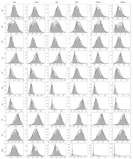
Figure 8.
Histograms of the surface reflectance in the different 10 land classes for the selected six Landsat 9 bands.
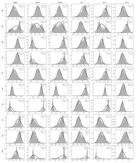
Figure 9.
Histograms of the Landsat 9 spectral indices (NDBI, NDVI, NDWI) and principal components (PC-1, PC-2, PC-3) for the 10 land classes.
The histograms of the Landsat image reveal that the reflectance of different urban formations in the blue, green, and red bands are almost like that of FL and HT. However, there is some variation in reflectivity among the classes of interest in the NIR, SWIR-1, and SWIR-2 bands. The histograms of PC-3 show a significant degree of variation between the DU and HT, whereas the histograms of other principal components demonstrate a noticeable difference between the DU and HT. As SU has only a few nonurban pixels, the small range of reflectance values falls within the range of FL and HT. The distinguishable difference in reflectivity of VU, DV, and SV can be observed in NIR and SWIR-2. Similarly, the histograms of NDVI, NDBI, PC-1, and PC-2 clearly depict good variation between the classes.
All classifiers were successful in accurately classifying the DU subset using all methods, shown in Figure 10. For methods 1 and 4, both CART and RF were able to effectively extract roads in the RU subset. However, the quantitative analysis of the RU and SV subsets yielded unsatisfactory results.
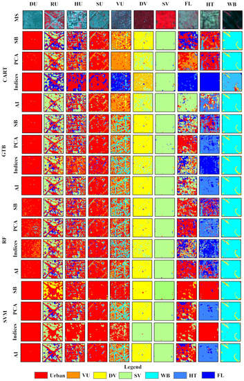
Figure 10.
Classification results for scenario-based analysis from Landsat 9 image using the 4 input methods (method 1: SB; method 2: indices; method 3: PCA; method 4: AI) and SVM, FR, GTB, and CART classifiers in a scenario-based approach. The first row (MS) refers to the false color subset image.
Although SVM produced a TA of 79.44% in method 1, it was unable to correctly identify the nonurban regions in the SU patch. The HU areas subset presented a challenge due to the high building height, which resulted in adjacent pixels being obscured by shadow, creating a shadow effect. Several classifiers misclassified the shadow region as WB, as the reflectance of the shadow region resembled that of a body of water.
In method 4, the performance of classifiers in identifying urban and rural areas was improved by using the PC components in the SU subset. Similarly, the accuracy of classification for the SV, DV, and HT subsets was enhanced by employing PCA. The classifiers, except for CART, were found to be effective in identifying the WB when indices were added. In method 1, only the GTB classifier could identify the FL, while adding indices to method 4 improved the classification accuracy of GTB and RF in identifying fallow land. However, using spectral indices led to a decrease in classification accuracy for CART and SVM, which was rectified by including all inputs in method 4.
5.2.2. Analysis with Sentinel Image
Figure 11 and Figure 12 display histograms representing the observed surface reflectance from the selected six bands of Sentinel imagery and histograms of the generated indices (NDBI, NDVI, and NDWI) and principal components (PC-1, PC-2, and PC-3) derived from the same Sentinel imagery.
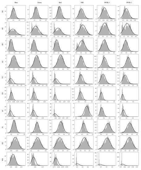
Figure 11.
Histograms of the surface reflectance in the different 10 classes for the selected six Sentinel bands.
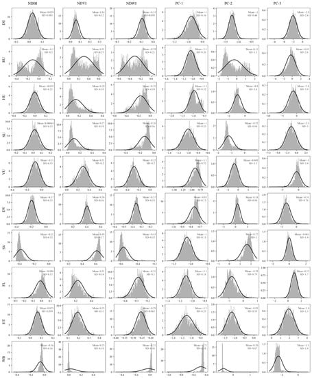
Figure 12.
Histograms of the Sentinel-2 spectral indices (NDBI, NDVI, NDWI) and principal components (PC-1, PC-2, PC-3) for the 10 land classes.
The histograms plotted for the blue, green, red, and SWIR-2 Sentinel image bands (Figure 11) did not reveal any significant differences in reflectivity between the different vegetation classes such as VU, DV, and SV. Moreover, FL and HT were found to be falling within the range of urban classes. However, there was a discernible variation between the classes of interest in the NIR and SWIR-1 bands. On the other hand, the indices and principal components derived from the Sentinel image bands showed distinguishable variations, except for NDBI and PC-1. NDVI, NDWI, and PC-2 exhibited slight differences in reflectance between VU, DV, and SV. Similarly, NDWI and PC-3 demonstrated the variation in reflectance between urban classes, FL, and HT (Figure 12).
Figure 13 provides the classification results of the Sentinel image for qualitative analysis. All the machine learning classifiers used in the SV subset performed well with each of the input methods. The use of PCA in method 4 improved the classification accuracy of HT and DV when combined with other bands. Except for SVM with indices, all classifiers were able to accurately extract WB and RU in all methods. However, due to shadows, the high-rise buildings were mistakenly classified as WB, and the use of indices helped CART improve the accuracy of the HU class.
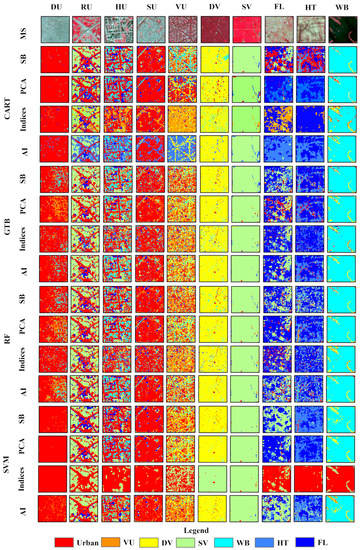
Figure 13.
Classification results for scenario-based analysis from Sentinel-2 image using the 4 input methods (method 1: SB; method 2: indices; method 3: PCA; method 4: AI) and SVM, FR, GTB, and CART classifiers in a scenario-based approach. The first row (MS) refers to the false color subset image.
Compared to other techniques, the use of spectral indices significantly improved the classifier’s ability to distinguish between urban and FL classes. The CART classifier performed well in the DU, DV, SV, and WB classes in all input scenarios. It accurately extracted roads in urban areas and was able to identify roads between mixed urban and vegetation areas, which other classifiers were unable to do. There were no significant differences in the outcomes of the GTB classifier when different input scenarios were used, but without PCA, a small number of pixels in the DU class were incorrectly labeled as WB. The RF classifier performed well in almost all cases but had difficulty identifying the road between VU. In contrast, SVM performed the worst across all classes with the spectral indices, labeling almost all classes as DU.
6. Discussion
The previous research comparing different ML algorithms [71,72,73] highlighted that RF achieved the highest classification accuracy, which is consistent with our findings in quantitative analysis. RF, along with GTB, consistently demonstrated good performance across all input configurations. Furthermore, methods 1 and 4 exhibited the highest classification accuracy overall. Similar to the previous research mentioned, other classifiers such as CART, SVM, and MD followed in terms of accuracy assessment. Our study also demonstrated that the inclusion of spectral indices and PCA, along with multispectral bands in method 4, improved the validation accuracy.
Notably, there are limited studies that discuss the role of PCA in classification with sensors. Our study revealed that using principal component bands from high-resolution images such as Sentinel-2 in the GTB classifier can enhance the validation accuracy. Additionally, the SVM classifier performed better than other classifiers when used with PCA bands in method 3. However, it is worth mentioning that Naive Bayes (NB) showed poor accuracy and was unable to perform well only with PCA. Our study found that using spectral indices alone reduced the classification accuracy, whereas incorporating PCA helped improve the accuracy of most classifiers. Many studies traditionally have relied on thresholding spectral indices for feature extraction, but our study results indicate that using spectral indices alone in ML classifiers can lead to misclassification and reduce classification accuracy.
Although previous research has extensively analyzed classifier performance at the comprehensive class [74,75,76], there is a notable gap in assessing classifier performance at the targeted feature, which is crucial when focusing on targeted feature classes. The effectiveness of classifiers varies depending on the feature classes, even though many classifiers demonstrate satisfactory accuracy in quantitative analysis. The incorporation of PCA proves highly advantageous for classifiers as it enables them to identify even the slightest differences within a subset. On the other hand, spectral indices are useful for categorizing easily distinguishable classes. However, their inclusion in multiple classifiers has resulted in redundancy and reduced classification accuracy. Previous studies have highlighted the challenge of accurately classifying fallow land and urban areas due to their similar reflectance properties. However, the targeted feature analysis in our study reveals that the inclusion of spectral indices and PCA with the multispectral bands can effectively differentiate these classes, outperforming other methods. It is worth noting that distinguishing fallow land and urban areas is easier in Sentinel images compared to Landsat images. In dense urban areas, slight variations on the surface can lead to the misclassification of shadow or road pixels as water bodies by some classifiers.
The study focused on a specific set of classifiers and input combinations: a limitation of the proposed analysis is the extension of the sample size used for training and testing, since a larger sample size would provide more robust and general results. The selection and configuration of hyperparameters can impact classification accuracy, and there is a possibility of suboptimal parameter selection. Exploring other classifiers and input configurations would provide further insights. The study focused primarily on urban areas, and the performance of classifiers may differ for other land cover classes. Furthermore, temporal variations in satellite imagery were not addressed, which could affect land cover classification accuracy. Future research should consider these limitations and explore classification performance across different land cover classes and temporal dynamics.
The analysis provides insights into the usefulness of combining different inputs, all derived from surface reflectance satellite observations, for land cover classification machine learning algorithms. The use of images from two different satellites, i.e., Landsat 9 and Sentinel-2, also provides further insight into the sensor-based variability of the methodology and classifier performance. The overall results are based on a specific study area and on images acquired in March 2022: therefore, this analysis is the first assessment of the proposed methodology and classifier comparison, which should be evaluated in future research over other areas and considering images in different seasons.
7. Conclusions
This study focused on evaluating the performance of various machine learning classifiers for land cover classification using remote sensing data. The analysis included different input combinations, such as multispectral bands, spectral indices, and principal component analysis. The goal was to determine the most effective classifiers and input methods for accurately classifying land cover features. The study also examined the classifiers’ accuracy at both the comprehensive feature and targeted feature class. The findings revealed that the inclusion of PCA and spectral indices significantly improved the accuracy of the classifiers in differentiating between land cover classes. Method 1, which used only satellite bands, and method 4, which combined satellite bands, indices, and PCA, achieved the highest classification accuracy. Among the classifiers assessed, Random Forest and Gradient Boosted Trees consistently demonstrated superior performance across all input methods. The use of high-resolution Sentinel-2 images proved advantageous in identifying targeted land cover classes, such as fallow land, and distinguishing between urban and barren areas. However, certain classifiers struggled with a misclassifying shadow or road pixels as water bodies. The study highlights the importance of conducting feature-specific analysis when using classification results for subsequent applications. It also emphasizes the potential benefits of incorporating additional statistically derived input variables to enhance classification accuracy.
Author Contributions
Conceptualization, P.A.P.; methodology, P.A.P. and K.J.; validation, P.A.P. and K.J.; formal analysis, P.A.P., K.J. and S.B.; writing—original draft preparation, P.A.P.; writing—review and editing, P.A.P., K.J. and S.B.; supervision, K.J. and S.B. All authors have read and agreed to the published version of the manuscript.
Funding
This research received no external funding.
Data Availability Statement
The data supporting this study’s findings are available from the corresponding author upon reasonable request.
Acknowledgments
The authors would like to extend their gratitude to the Indian Institute of Technology, Roorkee, for providing access to their resources, which were essential in conducting this research. Additionally, the authors would like to express their appreciation to the anonymous reviewers for their insightful and constructive feedback, which greatly helped in improving the overall quality of this work.
Conflicts of Interest
This manuscript has not been published or presented elsewhere in part or in entirety and is not under consideration by another journal. There are no conflicts of interest to declare.
References
- Twisa, S.; Buchroithner, M.F. Land-use and land-cover (LULC) change detection in Wami river basin, Tanzania. Land 2019, 8, 136. [Google Scholar] [CrossRef]
- De Souza, J.M.; Morgado, P.; da Costa, E.M.; de Vianna, N.L.F. Modeling of Land Use and Land Cover (LULC) Change Based on Artificial Neural Networks for the Chapecó River Ecological Corridor, Santa Catarina/Brazil. Sustainability 2022, 14, 4038. [Google Scholar] [CrossRef]
- Prathiba, A.P.; Rastogi, K.; Jain, G.V.; Kumar, V.V.G. Building Footprint Extraction from Very-High-Resolution Satellite Image Using Object-Based Image Analysis (OBIA) Technique. Lect. Notes Civ. Eng. 2020, 33, 517–529. [Google Scholar] [CrossRef]
- Sharma, S.K.; Kumar, M.; Maithani, S.; Kumar, P. Feature Extraction in Urban Areas Using UAV Data; Springer International Publishing: Cham, Switzerland, 2023; pp. 87–98. [Google Scholar] [CrossRef]
- Merugu, S.; Tiwari, A.; Sharma, S.K. Spatial–Spectral Image Classification with Edge Preserving Method. J. Indian Soc. Remote Sens. 2021, 49, 703–711. [Google Scholar] [CrossRef]
- Mishra, V.; Avtar, R.; Prathiba, A.; Mishra, P.K.; Tiwari, A.; Sharma, S.K.; Singh, C.H.; Chandra Yadav, B.; Jain, K. Uncrewed Aerial Systems in Water Resource Management and Monitoring: A Review of Sensors, Applications, Software, and Issues. Adv. Civ. Eng. 2023, 2023, 3544724. [Google Scholar] [CrossRef]
- Shukla, A.; Jain, K. Automatic extraction of urban land information from unmanned aerial vehicle (UAV) data. Earth Sci. Inform. 2020, 13, 1225–1236. [Google Scholar] [CrossRef]
- Dibs, H.; Hasab, H.A.; Mahmoud, A.S.; Al-Ansari, N. Fusion Methods and Multi-classifiers to Improve Land Cover Estimation Using Remote Sensing Analysis. Geotech. Geol. Eng. 2021, 39, 5825–5842. [Google Scholar] [CrossRef]
- Sinha, S.; Sharma, L.K.; Nathawat, M.S. Improved Land-use/Land-cover classification of semi-arid deciduous forest landscape using thermal remote sensing. Egypt. J. Remote Sens. Space Sci. 2015, 18, 217–233. [Google Scholar] [CrossRef]
- Zha, Y.; Gao, J.; Ni, S. Use of normalized difference built-up index in automatically mapping urban areas from TM imagery. Int. J. Remote Sens. 2003, 24, 583–594. [Google Scholar] [CrossRef]
- Prathiba, A.P.; Jain, K. Geospatial Landscape Analysis of an Urban Agglomeration: A Case Study of National Capital Region of India. In Proceedings of the 2021 IEEE International Geoscience and Remote Sensing Symposium IGARSS, Brussels, Belgium, 11–16 July 2021; pp. 6371–6374. [Google Scholar] [CrossRef]
- Hais, M.; Jonášová, M.; Langhammer, J.; Kučera, T. Comparison of two types of forest disturbance using multitemporal Landsat TM/ETM+ imagery and field vegetation data. Remote Sens. Environ. 2009, 113, 835–845. [Google Scholar] [CrossRef]
- Kennedy, R.E.; Yang, Z.; Cohen, W.B. Detecting trends in forest disturbance and recovery using yearly Landsat time series: 1. LandTrendr—Temporal segmentation algorithms. Remote Sens. Environ. 2010, 114, 2897–2910. [Google Scholar] [CrossRef]
- Yang, X.; Lo, C.P. Using a time series of satellite imagery to detect land use and land cover changes in the Atlanta, Georgia metropolitan area. Int. J. Remote Sens. 2002, 23, 1775–1798. [Google Scholar] [CrossRef]
- Gao, B.-C. NDWI—A Normalized Difference Water Index for Remote Sensing of Vegetation Liquid Water from Space. Remote Sens. Environ. 1996, 58, 257–266. Available online: https://www.sciencedirect.com/science/article/pii/S0034425796000673 (accessed on 24 December 2020). [CrossRef]
- Ji, L.; Geng, X.; Sun, K.; Zhao, Y.; Gong, P. Target Detection Method for Water Mapping Using Landsat 8 OLI/TIRS Imagery. Water 2015, 7, 794–817. [Google Scholar] [CrossRef]
- Tang, P.; Huang, J.; Zhou, H.; Wang, H.; Huang, W.; Huang, X.; Yuan, Y. The spatiotemporal evolution of urbanization of the countries along the Belt and Road Initiative using the compounded night light index. Arab. J. Geosci. 2021, 14, 1677. [Google Scholar] [CrossRef]
- Chakraborty, A.; Sachdeva, K.; Joshi, P.K. Mapping long-term land use and land cover change in the central Himalayan region using a tree-based ensemble classification approach. Appl. Geogr. 2016, 74, 136–150. [Google Scholar] [CrossRef]
- Schubert, H.; Calvo, A.C.; Rauchecker, M.; Rojas-Zamora, O.; Brokamp, G.; Schütt, B. Article assessment of land cover changes in the hinterland of Barranquilla (Colombia) using landsat imagery and logistic regression. Land 2018, 7, 152. [Google Scholar] [CrossRef]
- Talukdar, S.; Singha, P.; Mahato, S.; Shahfahad; Pal, S.; Liou, Y.-A.; Rahman, A. Land-use land-cover classification by machine learning classifiers for satellite observations—A review. Remote Sens. 2020, 12, 1135. [Google Scholar] [CrossRef]
- Zeferino, L.B.; de Souza, L.F.T.; Amaral, C.H.; Filho, E.I.F.; de Oliveira, T.S. Does environmental data increase the accuracy of land use and land cover classification? Int. J. Appl. Earth Obs. Geoinf. 2020, 91, 102128. [Google Scholar] [CrossRef]
- Celik, T. Unsupervised change detection in satellite images using principal component analysis and κ-means clustering. IEEE Geosci. Remote Sens. Lett. 2009, 6, 772–776. [Google Scholar] [CrossRef]
- Nasr, A.H.; El-Samie, F.E.A.; Metwalli, M.R.; Allah, O.S.F.; El-Rabaie, S. Satellite image fusion based on principal component analysis and high-pass filtering. JOSA A 2010, 27, 1385–1394. [Google Scholar] [CrossRef]
- Aldhshan, S.R.S.; Shafri, H.Z.M. Change detection on land use/land cover and land surface temperature using spatiotemporal data of Landsat: A case study of Gaza Strip. Arab. J. Geosci. 2019, 12, 443. [Google Scholar] [CrossRef]
- Dou, P.; Chen, Y. Remote sensing imagery classification using adaboost with a weight vector (WV adaboost). Remote Sens. Lett. 2017, 8, 733–742. [Google Scholar] [CrossRef]
- Dutta, D.; Rahman, A.; Paul, S.K.; Kundu, A. Changing pattern of urban landscape and its effect on land surface temperature in and around Delhi. Environ. Monit. Assess. 2019, 191, 551. [Google Scholar] [CrossRef]
- Mishra, V.N.; Prasad, R.; Rai, P.K.; Vishwakarma, A.K.; Arora, A. Performance evaluation of textural features in improving land use/land cover classification accuracy of heterogeneous landscape using multi-sensor remote sensing data. Earth Sci. Inform. 2019, 12, 71–86. [Google Scholar] [CrossRef]
- Alifu, H.; Vuillaume, J.F.; Johnson, B.A.; Hirabayashi, Y. Machine-learning classification of debris-covered glaciers using a combination of Sentinel-1/-2 (SAR/optical), Landsat 8 (thermal) and digital elevation data. Geomorphology 2020, 369, 107365. [Google Scholar] [CrossRef]
- Avudaiammal, R.; Elaveni, P.; Selvan, S.; Rajangam, V. Extraction of Buildings in Urban Area for Surface Area Assessment from Satellite Imagery based on Morphological Building Index using SVM Classifier. J. Indian Soc. Remote Sens. 2020, 48, 1325–1344. [Google Scholar] [CrossRef]
- Maxwell, A.E.; Warner, T.A.; Fang, F. Implementation of machine-learning classification in remote sensing: An applied review. Int. J. Remote Sens. 2018, 39, 2784–2817. [Google Scholar] [CrossRef]
- Szuster, B.W.; Chen, Q.; Borger, M. A comparison of classification techniques to support land cover and land use analysis in tropical coastal zones. Appl. Geogr. 2011, 31, 525–532. [Google Scholar] [CrossRef]
- Bar-Hen, A.; Gey, S.; Poggi, J.-M. Influence Measures for CART Classification Trees. J. Classif. 2015, 32, 21–45. [Google Scholar] [CrossRef]
- Hu, Y.Y.; Hu, Y.Y. Land cover changes and their driving mechanisms in Central Asia from 2001 to 2017 supported by Google Earth Engine. Remote Sens. 2019, 11, 554. [Google Scholar] [CrossRef]
- Sang, X.; Guo, Q.Z.; Wu, X.X.; Fu, Y.; Xie, T.Y.; Wei, H.C.; Zang, J.L. Intensity and stationarity analysis of land use change based on cart algorithm. Sci. Rep. 2019, 9, 12279. [Google Scholar] [CrossRef]
- Wang, S.; Ma, Q.; Ding, H.; Liang, H. Detection of urban expansion and land surface temperature change using multi-temporal landsat images. Resour. Conserv. Recycl. 2018, 128, 526–534. [Google Scholar] [CrossRef]
- Cao, F.; Liu, F.; Guo, H.; Kong, W.; Zhang, C.; He, Y. Fast detection of sclerotinia sclerotiorum on oilseed rape leaves using low-altitude remote sensing technology. Sensors 2018, 18, 4464. [Google Scholar] [CrossRef]
- Elmahdy, S.I.; Ali, T.A.; Mohamed, M.M.; Howari, F.M.; Abouleish, M.; Simonet, D. Spatiotemporal Mapping and Monitoring of Mangrove Forests Changes From 1990 to 2019 in the Northern Emirates, UAE Using Random Forest, Kernel Logistic Regression and Naive Bayes Tree Models. Front. Environ. Sci. 2020, 8, 102. [Google Scholar] [CrossRef]
- Lv, Z.Y.; He, H.; Benediktsson, J.A.; Huang, H. A generalized image scene decomposition-based system for supervised classification of very high resolution remote sensing imagery. Remote Sens. 2016, 8, 814. [Google Scholar] [CrossRef]
- Li, C.F.; Yin, J.Y. Variational Bayesian independent component analysis-support vector machine for remote sensing classification. Comput. Electr. Eng. 2013, 39, 717–726. [Google Scholar] [CrossRef]
- Tong, X.; Zhang, X.; Liu, M. Detection of urban sprawl using a genetic algorithm-evolved artificial neural network classification in remote sensing: A case study in Jiading and Putuo districts of Shanghai, China. Int. J. Remote Sens. 2010, 31, 1485–1504. [Google Scholar] [CrossRef]
- Yang, B.; Cao, C.; Xing, Y.; Li, X. Automatic Classification of Remote Sensing Images Using Multiple Classifier Systems. Math. Probl. Eng. 2015, 2015, 954086. [Google Scholar] [CrossRef]
- Zhong, Y.; Zhang, L.; Gong, J.; Li, P. A supervised artificial immune classifier for remote-sensing imagery. IEEE Trans. Geosci. Remote Sens. 2007, 45, 3957–3966. [Google Scholar] [CrossRef]
- Chen, B.; Huang, B.; Xu, B. Multi-source remotely sensed data fusion for improving land cover classification. ISPRS J. Photogramm. Remote Sens. 2017, 124, 27–39. [Google Scholar] [CrossRef]
- Carranza-García, M.; García-Gutiérrez, J.; Riquelme, J.C. A framework for evaluating land use and land cover classification using convolutional neural networks. Remote Sens. 2019, 11, 274. [Google Scholar] [CrossRef]
- Karimi, F.; Sultana, S.; Babakan, A.S.; Suthaharan, S. An enhanced support vector machine model for urban expansion prediction. Comput. Environ. Urban Syst. 2019, 75, 61–75. [Google Scholar] [CrossRef]
- Schmidt, G.; Jenkerson, C.; Masek, J.; Vermote, E.; Gao, F. Landsat Ecosystem Disturbance Adaptive Processing System (LEDAPS) Algorithm Description; USGS: Baltimore, MD, USA, 2013. Available online: http://www.usgs.gov/pubprod (accessed on 18 August 2022).
- Deng, C.; Zhu, Z. Continuous subpixel monitoring of urban impervious surface using Landsat time series. Remote Sens. Environ. 2020, 238, 110929. [Google Scholar] [CrossRef]
- Bouzekri, S.; Lasbet, A.A.; Lachehab, A. A New Spectral Index for Extraction of Built-Up Area Using Landsat-8 Data. J. Indian Soc. Remote Sens. 2015, 43, 867–873. [Google Scholar] [CrossRef]
- Hashim, H.; Latif, Z.A.; Adnan, N.A. Urban vegetation classification with NDVI threshold value method with very high resolution (VHR) Pleiades imagery. Int. Arch. Photogramm. Remote Sens. Spat. Inf. Sci. ISPRS Arch. 2019, 42, 237–240. [Google Scholar] [CrossRef]
- Ibrahim, G.R.F. Urban land use land cover changes and their effect on land surface temperature: Case study using Dohuk City in the Kurdistan Region of Iraq. Climate 2017, 5, 13. [Google Scholar] [CrossRef]
- Phan, T.N.; Kuch, V.; Lehnert, L.W. Land cover classification using google earth engine and random forest classifier-the role of image composition. Remote Sens. 2020, 12, 2411. [Google Scholar] [CrossRef]
- Xu, H. Modification of normalised difference water index (NDWI) to enhance open water features in remotely sensed imagery. Int. J. Remote Sens. 2006, 27, 3025–3033. [Google Scholar] [CrossRef]
- Fowler, J.E. Compressive-projection principal component analysis. IEEE Trans. Image Process. 2009, 18, 2230–2242. [Google Scholar] [CrossRef]
- Cao, X.; Gao, X.; Shen, Z.; Li, R. Expansion of Urban Impervious Surfaces in Xining City Based on GEE and Landsat Time Series Data. IEEE Access 2020, 8, 147097–147111. [Google Scholar] [CrossRef]
- Adepoju, K.A.; Adelabu, S.A. Improving accuracy evaluation of Landsat-8 OLI using image composite and multisource data with Google Earth Engine. Remote Sens. Lett. 2020, 11, 107–116. [Google Scholar] [CrossRef]
- Phalke, A.R.; Özdoğan, M.; Thenkabail, P.S.; Erickson, T.; Gorelick, N.; Yadav, K.; Congalton, R.G. Mapping croplands of Europe, Middle East, Russia, and Central Asia using Landsat, Random Forest, and Google Earth Engine. ISPRS J. Photogramm. Remote Sens. 2020, 167, 104–122. [Google Scholar] [CrossRef]
- Vapnik, V.N. The Nature of Statistical Learning Theory; Springer: New York, NY, USA, 1995. [Google Scholar]
- Wolfowitz, J. Estimation by the Minimum Distance Method in Nonparametric Stochastic Difference Equations. Ann. Math. Stat. 1954, 25, 203–217. [Google Scholar] [CrossRef]
- Breiman, L.; Friedman, J.H.; Olshen, R.A.; Stone, C.J. Classification and Regression Trees. Biometrics 1984, 40, 874. [Google Scholar] [CrossRef]
- Hu, D.; Chen, S.; Qiao, K.; Cao, S. Integrating CART algorithm and multi-source remote sensing data to estimate sub-pixel impervious surface coverage: A case study from Beijing Municipality, China. Chinese Geogr. Sci. 2017, 27, 614–625. [Google Scholar] [CrossRef]
- Wang, J.; Wu, Z.; Wu, C.; Cao, Z.; Fan, W.; Tarolli, P. Improving impervious surface estimation: An integrated method of classification and regression trees (CART) and linear spectral mixture analysis (LSMA) based on error analysis. GIScience Remote Sens. 2018, 55, 583–603. [Google Scholar] [CrossRef]
- Pelletier, C.; Valero, S.; Inglada, J.; Champion, N.; Dedieu, G. Assessing the robustness of Random Forests to map land cover with high resolution satellite image time series over large areas. Remote Sens. Environ. 2016, 187, 156–168. [Google Scholar] [CrossRef]
- Rodriguez-Galiano, V.F.; Ghimire, B.; Rogan, J.; Chica-Olmo, M.; Rigol-Sanchez, J.P. An assessment of the effectiveness of a random forest classifier for land-cover classification. ISPRS J. Photogramm. Remote Sens. 2012, 67, 93–104. [Google Scholar] [CrossRef]
- Tong, X.; Brandt, M.; Hiernaux, P.; Herrmann, S.; Rasmussen, L.V.; Rasmussen, K.; Tian, F.; Tagesson, T.; Zhang, W.; Fensholt, R. The forgotten land use class: Mapping of fallow fields across the Sahel using Sentinel-2. Remote Sens. Environ. 2020, 239, 111598. [Google Scholar] [CrossRef]
- Zurqani, H.A.; Post, C.J.; Mikhailova, E.A.; Schlautman, M.A.; Sharp, J.L. Geospatial analysis of land use change in the Savannah River Basin using Google Earth Engine. Int. J. Appl. Earth Obs. Geoinf. 2018, 69, 175–185. [Google Scholar] [CrossRef]
- Yu, B.; Chen, C.; Zhou, H.; Liu, B.; Ma, Q. Prediction of Protein-Protein Interactions Based on L1-Regularized Logistic Regression and Gradient Tree Boosting. bioRxiv 2020. [Google Scholar] [CrossRef]
- Sachdeva, S.; Bhatia, T.; Verma, A.K. A novel voting ensemble model for spatial prediction of landslides using GIS. Int. J. Remote Sens. 2020, 41, 929–952. [Google Scholar] [CrossRef]
- Orieschnig, C.A.; Belaud, G.; Venot, J.-P.; Massuel, S.; Ogilvie, A. Input imagery, classifiers, and cloud computing: Insights from multi-temporal LULC mapping in the Cambodian Mekong Delta. Eur. J. Remote Sens. 2021, 54, 398–416. [Google Scholar] [CrossRef]
- Eddin, S.; Jozdani, B.; Johnson, A.; Chen, D. Comparing Deep Neural Networks, Ensemble Classifiers, and Support Vector Machine Algorithms for Object-Based Urban Land Use/Land Cover Classification. Remote Sens. 2019, 11, 1713. [Google Scholar]
- Abdi, A.M. Land cover and land use classification performance of machine learning algorithms in a boreal landscape using Sentinel-2 data. GIScience Remote Sens. 2020, 57, 1–20. [Google Scholar] [CrossRef]
- Zhou, L.; Luo, T.; Du, M.; Chen, Q.; Liu, Y.; Zhu, Y.; He, C.; Wang, S.; Yang, K. Machine Learning Comparison and Parameter Setting Methods for the Detection of Dump Sites for Construction and Demolition Waste Using the Google Earth Engine. Remote Sens. 2021, 13, 787. [Google Scholar] [CrossRef]
- Del Valle, T.M.; Jiang, P. Comparison of common classification strategies for large-scale vegetation mapping over the Google Earth Engine platform. Int. J. Appl. Earth Obs. Geoinf. 2022, 115, 103092. [Google Scholar] [CrossRef]
- Sackdavong, M.; Akitoshi, H. Comparison of Machine Learning Classifiers for Land Cover Changes using Google Earth Engine. In Proceedings of the 2021 IEEE International Conference on Aerospace Electronics and Remote Sensing Technology (ICARES), Bali, Indonesia, 3–4 November 2021; Available online: https://ieeexplore.ieee.org/stamp/stamp.jsp?tp=&arnumber=9665186&tag=1 (accessed on 3 May 2023).
- Sultana, S.; Satyanarayana, A.N.V. Assessment of urbanisation and urban heat island intensities using landsat imageries during 2000–2018 over a sub-tropical Indian City. Sustain. Cities Soc. 2020, 52, 101846. [Google Scholar] [CrossRef]
- Tiwari, A.; Tyagi, D.; Sharma, S.K.; Suresh, M.; Jain, K. Multi-criteria decision analysis for identifying potential sites for future urban development in Haridwar, India. Lect. Notes Electr. Eng. 2019, 500, 761–777. [Google Scholar] [CrossRef]
- Zhang, H.; Qi, Z.; Ye, X.; Cai, Y.; Ma, W.; Chen, M. Analysis of land use/land cover change, population shift, and their effects on spatiotemporal patterns of urban heat islands in metropolitan Shanghai, China. Appl. Geogr. 2013, 44, 121–133. [Google Scholar] [CrossRef]


Disclaimer/Publisher’s Note: The statements, opinions and data contained in all publications are solely those of the individual author(s) and contributor(s) and not of MDPI and/or the editor(s). MDPI and/or the editor(s) disclaim responsibility for any injury to people or property resulting from any ideas, methods, instructions or products referred to in the content. |
© 2023 by the authors. Licensee MDPI, Basel, Switzerland. This article is an open access article distributed under the terms and conditions of the Creative Commons Attribution (CC BY) license (https://creativecommons.org/licenses/by/4.0/).