Article

Crop-Planting Area Prediction from Multi-Source Gaofen Satellite Images Using a Novel Deep Learning Model: A Case Study of Yangling District

1
College of Mechanical and Electronic Engineering, Northwest A&F University, Xianyang 712100, China
2
College of Information Engineering, Northwest A&F University, Xianyang 712100, China
3
College of Water Resources and Architectural Engineering, Northwest A&F University, Xianyang 712100, China
4
Shanghai Institute of Satellite Engineering, Shanghai 200000, China
*
Author to whom correspondence should be addressed.
Remote Sens. 2023, 15(15), 3792; https://doi.org/10.3390/rs15153792
Submission received: 16 May 2023 / Revised: 21 July 2023 / Accepted: 28 July 2023 / Published: 30 July 2023
(This article belongs to the Section Remote Sensing in Agriculture and Vegetation)

Abstract

:
Neural network models play an important role in crop extraction based on remote sensing data. However, when dealing with high-dimensional remote sensing data, these models are susceptible to performance degradation. In order to address the challenges associated with multi-source Gaofen satellite data, a novel method is proposed for dimension reduction and crop classification. This method combines the benefits of the stacked autoencoder network for data dimensionality reduction, and the convolutional neural network for classification. By leveraging the advantages of multi-dimensional remote sensing information, and mitigating the impact of dimensionality on the classification accuracy, this method aims to improve the effectiveness of crop classification. The proposed method was applied to the extraction of crop-planting areas in the Yangling Agricultural Demonstration Zone, using multi-temporal spectral data collected from the Gaofen satellites. The results demonstrate that the fusion network, which extracts low-dimensional characteristics, offers advantages in classification accuracy. At the same time, the proposed model is compared with methods such as the decision tree (DT), random forest (RF), support vector machine (SVM), hyperspectral image classification based on a convolutional neural network (HICCNN), and a characteristic selection classification method based on a convolutional neural network (CSCNN). The overall accuracy of the proposed method can reach 98.57%, which is 7.95%, 4.69%, 5.68%, 1.21%, and 1.10% higher than the above methods, respectively. The effectiveness of the proposed model was verified through experiments. Additionally, the model demonstrates a strong robustness when classifying based on new data. When extracting the crop area of the entire Yangling District, the errors for wheat and corn are only 9.6% and 6.3%, respectively, and the extraction results accurately reflect the actual planting situation of crops.

1. Introduction

The real-time and effective extraction of agricultural distribution is a crucial prerequisite to the efficient management of crop planting in precision agriculture [1,2,3]. Traditional approaches to obtaining crop-planting structures primarily involve field investigations or manual segmentation, in conjunction with high-definition satellite imagery. However, the efficiency of these methods is exceedingly low. In the case of planting types with complex crop structures, extensive coverage, and significant temporal changes, they are prone to human error, and cannot fulfill real-time requirements. In contrast, the utilization of automatic crop recognition using machines has been demonstrated to be an efficient and cost-effective alternative [4]. It also represents a vital direction for the advancement of precision agriculture.
Satellite remote sensing technology plays a crucial role in efficient land information acquisition. By employing appropriate backend data-processing techniques, it becomes possible to extract valuable agricultural information from satellite data [5,6,7,8,9]. This enables efficient and real-time crop identification [10,11,12,13,14,15,16,17,18,19,20]. Among them, machine learning (ML) and deep learning (DL) [21,22,23,24,25,26,27,28] methods have been proven effective in extracting agricultural information from remote sensing data. These methods (ML and DL) utilize feature learning to achieve target classification, leading to improved information extraction results. They have become one of the main approaches to obtaining crop distribution information. In the field of remote sensing image data analysis, ML methods, such as the support vector machine (SVM), random forest (RF), and decision tree (DT) have demonstrated practicality in various applications. These methods have been successfully utilized for tasks such as corn-planting-area extraction [15], ground-object-type classification [16], and crop classification [20]. The application of ML methods in agricultural information extraction tasks using remote sensing data has proven to be feasible and efficient. Furthermore, compared to traditional ML methods, DL methods, particularly the convolutional neural network (CNN), exhibit a superior ability to learn complex features [29]. Hu et al. [30] introduced a DL method called hyperspectral image classification based on CNN (HICCNN), which demonstrated excellent feature-learning capabilities in object classification. In their study of crop classification based on the Sentinel-2 dataset, Seydi et al. [25] proposed a method that combined CNN and a dual-attention module. This approach successfully classified various crop types, such as alfalfa, broad bean, wheat, barley, and rape, and achieved excellent classification results.
DL methods excel in performance by training model parameters with ample sample data. However, obtaining comprehensive and accurate ground truth distribution information can be challenging, especially in cases of complex crop-planting structures and scattered planting areas. This limitation results in a scarcity of training samples, hindering the classification ability of the model and, ultimately, impacting the accuracy of the crop-planting information extraction. To tackle this issue, one approach is to increase the amount of information available in the remote sensing data. By incorporating more dimensional information for training purposes, and fully utilizing the original remote sensing data, it becomes feasible to achieve a desirable classification accuracy with fewer samples [31,32]. Multi-temporal remote sensing images, acquired at different time points, capture temporal changes in crops, and provide valuable information in the time dimension [33,34,35,36]. Zhang et al. [37] demonstrated the enhanced accuracy of crop identification through the utilization of multi-temporal data, in a study based on Sentinel-2 data. Furthermore, leveraging data from multiple satellite sources can offer additional remote sensing information from diverse angles and bands.
Balancing the contradiction between the input data dimension and model performance degradation is crucial in achieving an optimal classification performance with limited samples. When dealing with high-dimensional data, the Hughes phenomenon [38] can arise if the input data have too many dimensions, thereby impacting the model’s performance. One effective approach to address this challenge is to utilize stacked autoencoder (SAE) networks, which excel in extracting low-dimensional characteristics [39,40,41,42]. The SAE network consists of multiple autoencoders, stacked and interconnected to extract low-dimensional features through an encoding and decoding process. Both SAE networks and the CNN operate on the principle of gradient-descent-based forward propagation, and error backward propagation. Therefore, combining the strengths of both approaches can result in a characteristic dimension reduction, and an improved classification performance. In this context, a model called the fused stacked autoencoder and convolutional neural network (FSACNN) is proposed, to facilitate the extraction of crop-planting areas. The FSACNN model can simultaneously perform data dimensionality reduction and classification tasks, leveraging the advantages of stacked autoencoders and the CNN.
In this study, the experiments were conducted in Yangling District, known for its abundant resources for wheat and corn cultivation. As a national agricultural demonstration zone, Yangling provides comprehensive and easily accessible data on the distribution and area of various crops, which greatly facilitated the implementation of the experiments, and the analysis of the data. Satellite images from Gaofen-1, 2, and 6, covering the research area, were obtained. With the use of these remote sensing data, a multi-temporal dataset was constructed, including spectral, texture, and vegetation indices, which served as inputs for the fusion network. The proposed model, along with DT, RF, SVM, HICCNN, and the characteristic selection classification based on a convolutional neural network (CSCNN) models, was employed to classify crops in the study area. Additionally, the study verified the classification advantages of the low-dimensional characteristics extracted by the proposed network.

2. Materials

2.1. Study Area

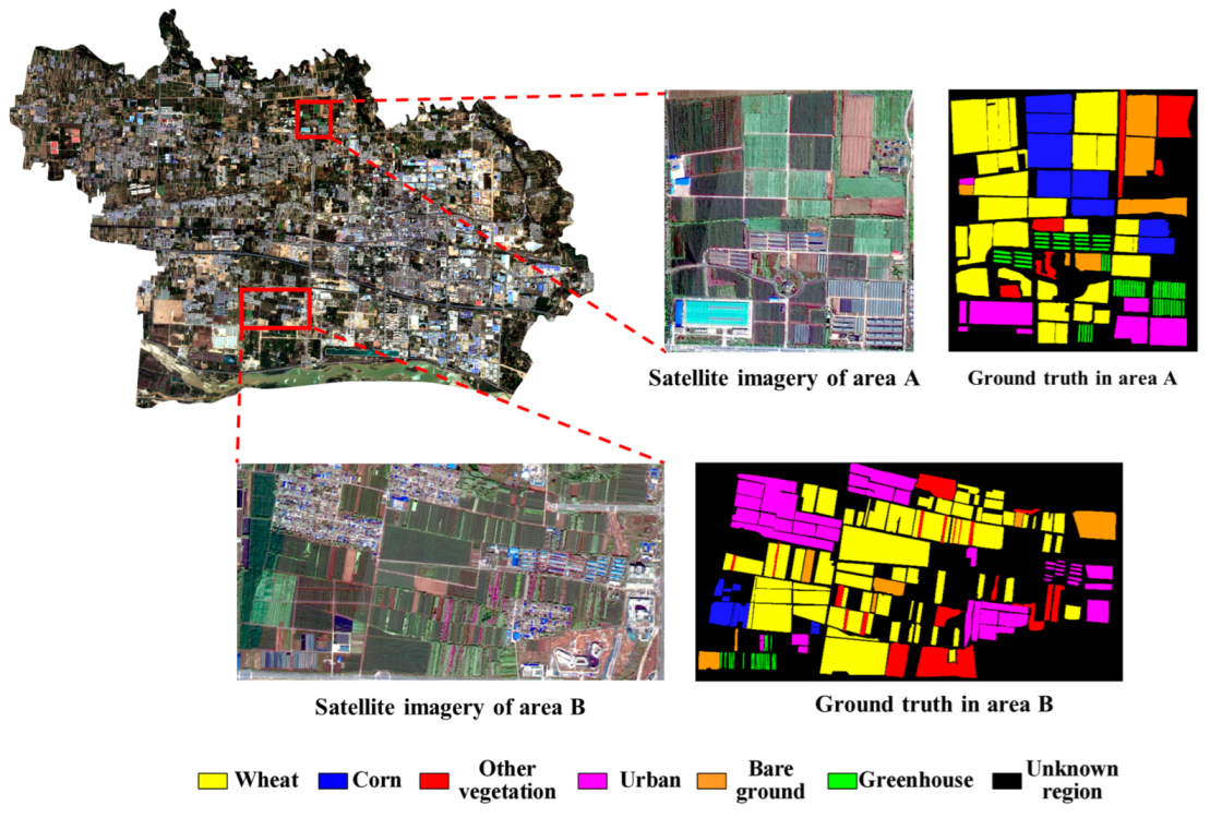
In this paper, the crop-planting area of Yangling Agricultural Demonstration Zone is extracted. Yangling is China’s first national agricultural high-tech industry demonstration zone, located in Shaanxi Province. The study area is depicted in Figure 1, where the red box represents the coverage range of a scene captured by the Gaofen-6 satellite.
The study area encompasses diverse land-cover types, encompassing crops, industrial crop plantations, residential houses, and greenhouses. The primary food crops cultivated are wheat and maize. For the purpose of this study, the land-cover types were classified into six categories: winter wheat, corn, other vegetation excluding winter wheat and corn (such as grassland and forest land), bare land, buildings (including urban and rural houses, and industrial plants), and greenhouses (including those covered with plastic mulch).

2.2. Dataset Selection and Data Processing

Due to cloud cover and rain, it is challenging for a single spectral satellite to obtain continuous and high-quality images. However, the use of multiple satellites can provide a wider range of information, through angle differences. Thus, for this study, multispectral images from Gaofen-1, Gaofen-2, and Gaofen-6 (GF-1, GF-2, and GF-6) were selected as the raw data. These satellites are optical remote sensing satellites that can capture images in the red, green, blue, near-infrared, and panchromatic bands [43,44]. The composite RGB (red, green, blue) image obtained by the three satellites is shown in Figure 2. The area circled in red represents the study area.
Based on the field investigation, it was observed that the color of the wheat crop gradually deepened as it entered the jointing and heading stage in April. This change made the crop characteristics more prominent, and facilitated the selection of the training samples in the satellite images. Consequently, the satellite images captured between April and June were carefully reviewed, and three cloud-free images were chosen as the multi-temporal data sources for the experiment. These images were acquired using the high-resolution cameras onboard the respective satellites, and their parameters [45] are presented in Table 1.
In the data acquisition process, each satellite provided a multispectral image with four bands (red, green, blue, and near-infrared), as well as a separate panchromatic image. Before further analysis, the acquired remote sensing data underwent pre-processing steps using ENVI software, to ensure the data were accurate and ready for subsequent analysis. Firstly, radiometric calibration, atmospheric correction, and orthographic correction were performed on the multispectral image of each temporal phase. Radiometric calibration is a crucial step in the processing of multispectral imagery. It involves converting the raw sensor measurements into physically meaningful units of radiance or reflectance. Following the radiometric calibration, atmospheric correction was applied, to account for the influence of the Earth’s atmosphere on the multispectral imagery. The orthographic correction aligned the image with a geographic coordinate system, ensuring spatial accuracy, and allowing for the precise measurement and analysis of features on the Earth’s surface. Then, the panchromatic images for each phase underwent radiometric correction, and orthophoto correction. For the radiometric calibration, the radiometric calibration tool in ENVI was utilized, to calibrate the panchromatic data to the atmospheric apparent reflectance. Subsequently, the radiometric calibrated data underwent orthophoto correction, using the “RPC Orthocorrection Workflow” tool in ENVI. Finally, the multispectral and panchromatic images were fused by Gram–Schmidt image fusion, to obtain the multispectral fusion image. The sampling rate of the pre-processed GF-1 and GF-6 images was 2 m, and the sampling rate of the GF-2 image was 0.8 m. In order not to lose image information, the GF-1 and GF-6 data were resampled to 0.8 m, and accurately matched with the GF-2 image.
In order to train a classification model, and accurately evaluate its classification accuracy, reliable ground truth data are necessary. However, due to the large size of the research area, obtaining complete ground truth data can be challenging. Therefore, sample data from two representative regions were selected for the model training. Through field investigations and the visual interpretation of high-resolution images, the distribution data of six land types were obtained. These land types included winter wheat, corn, other vegetation excluding winter wheat and corn (such as grassland and woodland), bare land, urban (including urban and rural houses, industrial plants, etc.), and greenhouse structures (made of plastic film or materials). Figure 3 displays the true distribution of these land types on the ground.
To construct the input data for the crop classification model, it is important to include characteristic information. This can be achieved by utilizing processed multi-spectral data to derive spectral characteristics. Additionally, incorporating textural characteristics in remote sensing image classification can be valuable in addressing the issue of “foreign objects with the same spectrum” in optical remote sensing image interpretation. Among the satellite images acquired, the GF-2 panchromatic image stood out, due to its highest spatial resolution, at 0.8 m, and prominent textural characteristics. Therefore, textural characteristics were extracted based on the GF-2 panchromatic images. The grey level co-occurrence matrix (GLCM) method, initially proposed by Haralick [46], is widely employed in image textural characteristic extraction. In this study, a set of 14 s-order statistics defined by GLCM are utilized to represent the extracted textures. Considering the correlation between the texture quantities and the computational requirements for high-resolution images, eight commonly used GLCM texture measures, namely the mean, variance, homogeneity, contrast, dissimilarity, entropy, angle second-order matrix, and correlation [46], were selected as the GLCM texture characteristics for this research.
The utilization of vegetation indices is highly effective in distinguishing between vegetation and non-vegetation areas, making this a promising approach to crop information extraction. By leveraging multispectral data, three specific vegetation indices can be calculated: the normalized differential vegetation index (NDVI), the ratio vegetation index (RVI), and the anthocyanin reflectance index 2 (ARI2). The NDVI is widely used to assess the growth status of vegetation [47]. On the other hand, the RVI serves as an indicator for measuring the vegetation growth and abundance [48]. The ARI2 is commonly utilized in vegetation health detection and crop yield analysis, among other applications. By combining the spectral characteristics, the GLCM textural characteristics, and the vegetation index characteristics, a 29-dimensional multi-temporal dataset is formed. Each characteristic is assigned a corresponding identifier for subsequent analysis. Table 2 provides a comprehensive list of all the characteristics, and their respective identifiers. The formula for calculating the three vegetation indices is given below:
N D V I = N I R R e d / N I R + R e d
R V I = N I R / R e d
A R I 2 = 2 × G r e e n B l u e R e d / 2 × G r e e n + B l u e + R e d
In Formula (1) to (3), NIR, Red, Green and Blue represent reflectance values of near-infrared band, red band, green band and blue band respectively.

3. Methodology

In this study, a crop classification model is developed, with the objective of improving classification accuracy, utilizing multi-dimensional characteristics, consisting of multi-temporal spectral data, textural characteristics, and vegetation index information, as the input for DL algorithms. The aim is to take advantage of the diverse information sources, to enhance the classification accuracy. Moreover, the high dimensionality of the input characteristics can lead to the Hughes phenomenon, a practical challenge where increasing the dimensionality of the data may result in a reduced classification performance. To address this issue, the SAE network is integrated with a CNN architecture. This integration effectively reduces the dimensionality of the data, while preserving the relevant information, resulting in a crop classification model with the ability to handle higher-dimensional input data.

3.1. Extraction Process of Crop-Planting Area

Figure 4 provides a flow chart illustrating the process of extracting the crop-planting areas. The first step involves preprocessing the satellite images obtained at each time phase. This preprocessing comprises radiometric calibration, atmospheric correction, orthographic correction, and image fusion. The registration and fusion are conducted simultaneously, to ensure accurate and merged images. Ground truth maps are created through field investigations and visual interpretation, using ENVI software. These ground truth maps serve as the reference for classification. Following this, the necessary classification characteristics are constructed as input data for the model. The final step involves training the model, using the constructed input data, and subsequently utilizing the trained model to classify crop-planting areas.

3.2. Data Dimensionality Reduction Method for Stacked Autoencoder Network

In the proposed method, the SAE is utilized as a multi-layer structure, consisting of interconnected simple autoencoders [42]. Figure 5 illustrates the structure of a single-layer autoencoder, comprising an input layer, an intermediate hidden layer, and an output layer. Notably, the data dimension of the intermediate hidden layer is smaller than that of the input layer. The purpose of the autoencoder is to reconstruct the input signal to match the output, through the supervised training of the parameters [42]. By performing this reconstruction, the autoencoder achieves an effective dimensionality reduction in the data in the intermediate hidden layer.
The dimensionality reduction is achieved through the following process. In the autoencoder, the input data are x = { x 1 , x 2 , , x n } , the intermediate hidden layer output is h = { h 1 , h 2 , , h m } , and the autoencoder output is y = { y 1 , y 2 , , y n } . The encoding and decoding process is as follows:
h = f ( W y x + b y )
y = g ( W z h + b z )
Here, f ( ) and g ( ) are the activation functions of the encoding and decoding process, which are generally sigmoid functions; W y are the weight matrices between the neurons in the input and middle layer; W z are the weight matrices between the neurons in the output and middle layer; b y is the bias between the neurons in the input and middle layer; and b z is the bias between the neurons in the output and middle layer. The autoencoder continuously trains the parameters W y , W z , b y , and b z by minimizing the loss function through the back propagation algorithm. The loss function is the mean-square error (MSE) between the output layer signals and the input layer signals. In this way, the autoencoder realizes the dimension reduction of the original input data, without reducing its ability for data information expression.
The SAE network is constructed by stacking multiple layers of single autoencoders, as depicted in Figure 6. Each layer of the autoencoder is trained individually, and the output of the previous layer serves as the input for the subsequent layer. This allows the network to form a model with an enhanced capability for extracting low-dimensional characteristics, compared to a single-layer autoencoder.

3.3. The Fusion Network Model of Stacked Autoencoder and CNN

Both the SAE and CNN networks share the fundamental principles of forward propagation and error backpropagation using gradient descent. This commonality in the training process provides a theoretical basis for network fusion. Taking advantage of the SAE network’s excellent data dimensionality reduction capability, and the CNN network’s classification advantages, an innovative network model that combines the SAE and CNN is constructed for the purpose of crop-planting area extraction. This model, known as the FSACNN, consists of four main parts: data input, data dimension reduction, characteristic extraction, and classification. The overall structure of the FSACNN method is presented in Figure 7. Before being fed into the fusion network, the SAE network is pre-trained. Subsequently, the data are inputted into the trained data dimension reduction component for dimensionality reduction, and the reduced-dimensional data are used as the input for the classification component. Simultaneously, the parameters of the data dimension reduction component are fine-tuned, by incorporating the classification results. This approach enables the organic integration of the two networks, resulting in an overall improved performance.
In the data dimensionality reduction part, the FSACNN method sequentially connects four autoencoders, to achieve dimensionality reduction in the multi-temporal remote sensing data. Once the dimension reduction is complete, the data can still be regarded as a sequence that maintains intra-class correlation. Therefore, one-dimensional convolution can be applied, to extract relevant characteristics from the data. This allows for effective feature extraction, and subsequent classification tasks.
In the feature extraction part of the FSACNN method, a three-branch parallel structure is constructed, using one-dimensional convolution, to enable the extraction of characteristics from different perception fields [49]. Considering the high correlation between adjacent points in the sequence, the first branch employs two convolutional layers, consisting of 1 × 3 convolution kernels, to extract the features that capture the relationships between neighboring points in depth. The second branch utilizes a single convolutional layer, with a 1 × 5 convolution kernel, to extract sequence characteristics over a broader range. The third branch incorporates a convolution layer with a 1 × 1 convolution kernel. This operation can be seen as the entire sequence passing through a fully connected layer, resulting in the sequence obtaining a single-point characteristic representation. Once the sequence characteristics have been extracted, using the respective convolutional layers, batch normalization operations and the linear rectifier function (ReLU) are applied, to process the data. This helps to normalize and activate the extracted features, respectively.
After the three-branch network structure, the Add operation is used, to accumulate the characteristic activation values extracted by the three branches and, finally, the probability results of all classes are obtained using the Soft-max classifier, to complete the classification. Meanwhile, the parameters of the dimension reduction part of the fusion model will be continuously optimized during the training process, to achieve a better data dimension reduction effect.

4. Experimental Results and Analysis

Firstly, regions A and B were classified. At this point, the experiment was conducted under two conditions: the training data belonged to the classification area, and they did not belong to the classification area. Subsequently, the performance of the dimensionality-reduced characteristics, and their impact on the model classification accuracy, were analyzed. Finally, the main crop areas in the entire study area were extracted.
The F1-score, overall classification accuracy (OA), and kappa coefficient (kappa) [50] were calculated, to evaluate the performance of the method. Among them, the F1-score was used as an evaluation index of a single category, and the OA and kappa were used as evaluation indicators for the overall classification. At the same time, the FSACNN method was compared with the DT, RF, SVM, HICCNN, and CSCNN methods. Among them, the CSCNN method used a correlation metric to automatically select the feature combination with the highest correlation to the sample label data. Then, these features were fed into the proposed CNN classification network for crop extraction. The parameter settings for the various methods were as follows. Decision trees: there was no maximum depth limitation, at least two samples were required for further node splitting, and the Gini coefficient was used for splitting. Random forests: construct random forests with 100 decision trees, consider the number of features equal to the square root of the total number of features when splitting nodes, and at least one sample was required in the leaf nodes. Support vector machines: the penalty strength was set to 1.0, the Gaussian radial basis function was used as the kernel function, and the reciprocal of the features was used as the gamma value. The loss function for the CSCNN, HICCNN, and FSACNN models was the cross-entropy function. The learning rate was set to 0.0001, and the training iterations were set to 300 times.

4.1. Condition 1: The Training Samples Belong to the Classification Area

In this experiment, both the training and test data were selected from the same experimental area. The training data for region A consisted of a random sampled 10% of each type of sample, while the crop-planting areas in region A were classified accordingly. Similarly, the crop-planting areas in region B were classified in the same manner. The obtained performance data for the different methods are presented in Table 3 and Table 4. Table 3 displays the classification accuracy of the various methods for region A, while Table 4 shows the classification accuracy for region B. Upon examining the tables, it becomes evident that the FSACNN, HICCNN and CSCNN methods outperform traditional ML methods, in terms of the accuracy for ground object classification within the two experimental areas. The CSCNN method with feature selection operation performs slightly better than the HICCNN. Notably, the FSACNN method exhibits a superior performance compared to the HICCNN and CSCNN methods. Indeed, this suggests that utilizing feature dimensionality reduction networks for feature optimization yields better results than simple feature selection methods, based on the correlation analysis. These findings demonstrate that the FSACNN method, in particular, improves the accuracy of ground object classification in both region A and region B, compared with traditional ML methods.
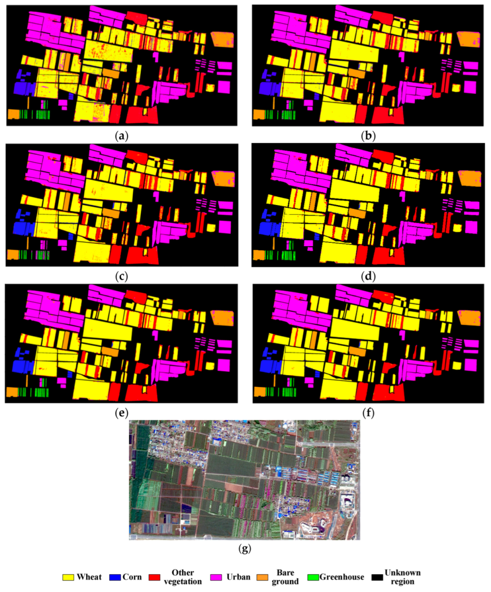
For region A, the OA and kappa coefficient of the FSACNN method reached 98.57% and 0.97, respectively, and the OA was increased by 7.95%, 4.69%, 5.68%, 1.21%, and 1.10%, respectively, compared with the DT, RF, SVM, HICCNN, and CSCNN. Compared with the DT, RF, SVM, HICCNN, and CSCNN, the kappa coefficient increased by 0.14, 0.09, 0.10, 0.03, and 0.01, respectively. For region B, the OA and kappa coefficient of the FSACNN method reached 97.76% and 0.94, respectively, and the OA was 9.72%, 5.74%, 6.53%, 2.50%, and 1.88% higher than the DT, RF, SVM, HICCNN, and CSCNN. Compared with the DT, RF, SVM, HICCNN, and CSCNN, the kappa coefficient was increased by 0.19, 0.14, 0.15, 0.06, and 0.02, respectively. Figure 8 and Figure 9, respectively, show the classification results for regions A and B, and the corresponding satellite imagery. Among the different methods, the classification results of the DT method (as shown in Figure 8a and Figure 9a) exhibit a noticeable “salt-and-pepper” phenomenon. This phenomenon can be attributed to the influence of “foreign matter with the same spectrum” between wheat, corn, and other vegetation types. As a result, the classification results for winter wheat and corn can become mixed with some other categories of vegetation. This issue leads to the blurring of boundaries between crop-planting areas and other types of vegetation, especially in plots that are adjacent to low-growing vegetation.
It can be seen from Figure 8b,c and Figure 9b,c that the classification results for the SVM and RF are similar to those of the HICCNN, CSCNN and FSACNN. However, there is still a considerable amount of mixed classification between wheat and other vegetation. The classification results obtained through the FSACNN method (Figure 8f and Figure 9f) demonstrate an overall reduction in salt-and-pepper noise. Additionally, the integrity of the distributed crop-planting area is good, and the extraction accuracy surpasses that of the HICCNN and CSCNN methods. This is because, compared with other methods, the FSACNN method utilizes its data dimensionality reduction ability to mitigate any negative impact that high-dimensional data may have on the model. Simultaneously, during the training process of the FSACNN method, the batch normalization operation is introduced, to standardize the input of each layer. This enables the network to continually adapt to new data distributions, and optimizes the training effect of the network. However, from an objective standpoint, it can be observed that the salt-and-pepper noise has not been entirely eliminated. Based on the classification results, although the proposed method exhibits a relatively reduced impact of salt-and-pepper noise compared to other methods, it is still slightly present.

4.2. Condition 2: The Training Samples Do Not Belong to the Classification Area

In order to further analyze the adaptability of the FSACNN method to new data, experiments were conducted using training samples that did not belong to the classification area. Region A was chosen for analysis, due to the uniformity of each ground-cover type in that area, which facilitated the analysis of the classification results. The model was trained using training data from region B, and the crop-planting area in region A was classified accordingly. The results are presented in Table 5 and Figure 10. Upon examining Table 5 and Figure 10 together, it becomes apparent that several methods experience a certain decline in prediction accuracy when predicting new data. Nonetheless, the FSACNN method still produced the most favorable results. The OA and kappa coefficients reached 87.15% and 0.83, respectively, while the F1-scores for wheat and corn reached 0.97 and 0.87, respectively.
Compared to the FSACNN method, both the DT and RF classifiers exhibited a lower classification accuracy. This can be attributed to the unbalanced distribution of training samples for each type, and the significant differences in characteristics between regions A and B. Additionally, Figure 10c reveals that the SVM struggles to effectively distinguish between greenhouses and architectural structures. Furthermore, referencing Table 3 and Table 5, it can be observed that when classifying new data, the proposed method experienced a decrease of 11.42% in the overall OA, and a decrease of 0.15 in the kappa coefficient. On the other hand, the HICCNN and CSCNN experiencd a decrease of 18.36% and 14.21% in the OA, and a decrease of 0.23 and 0.18 in the kappa coefficient. Therefore, the FSACNN method exhibits a stronger adaptability to new data, compared to the HICCNN and CSCNN. When it comes to classifying new data, the CSCNN performs slightly better than the HICCNN.
The aforementioned results demonstrate that the FSACNN method displays a high capability to differentiate various crops, vegetation, and other land-cover types. As a result, it offers a strong applicability in accurately extracting crop-planting areas from multi-temporal optical remote sensing data.

4.3. Performance Analysis of Characteristic Dimensionality Reduction

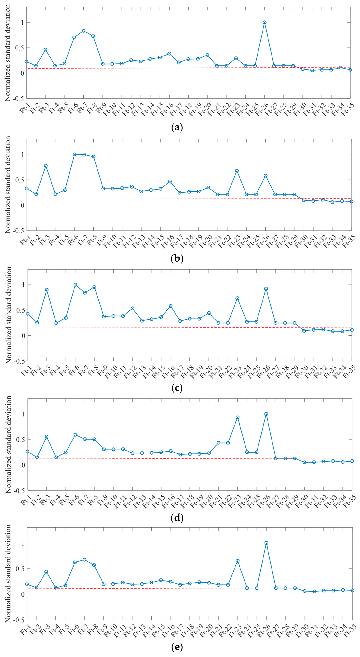
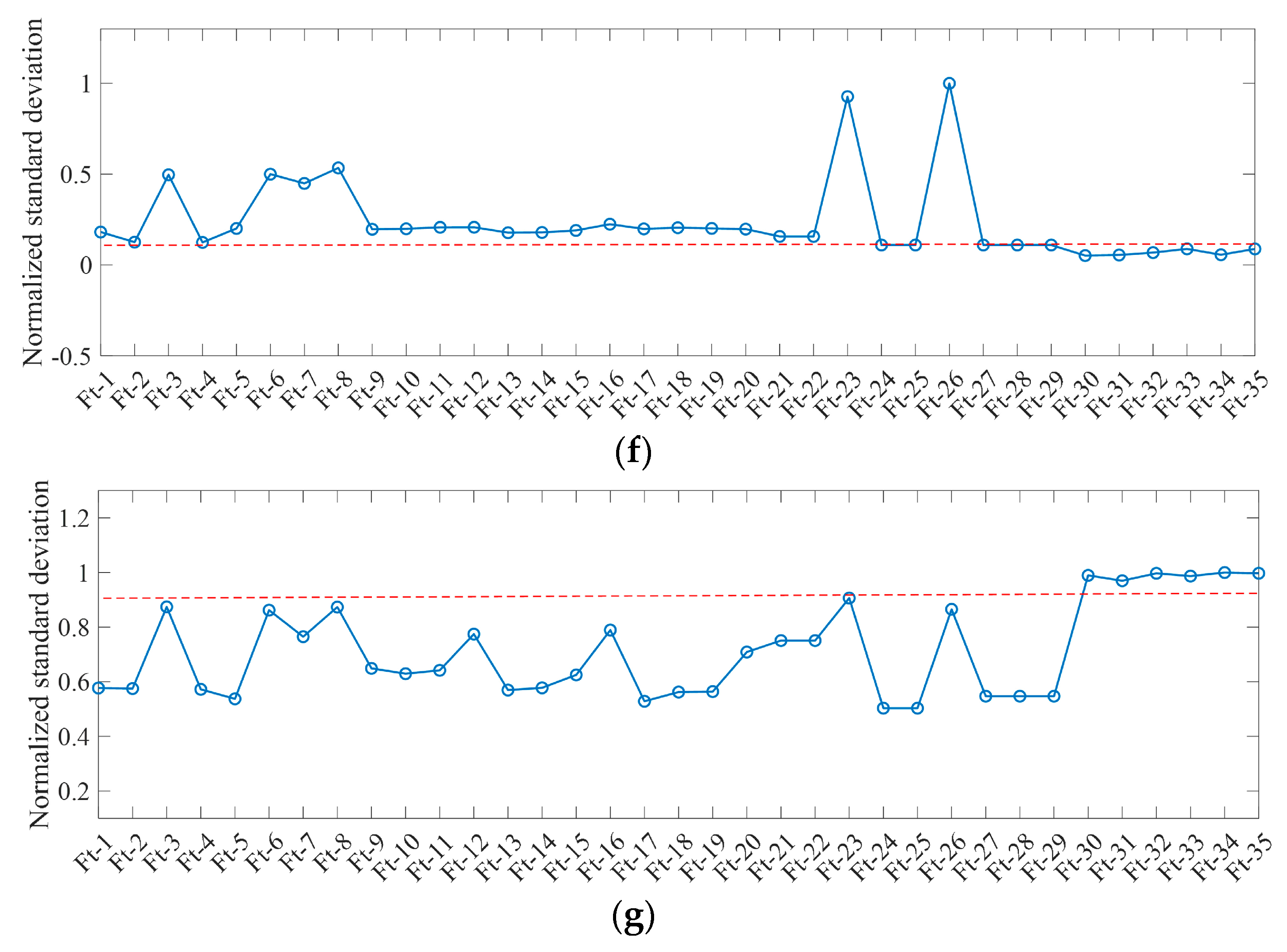
We randomly selected 10% of each class of samples from all the samples in region A plus region B as training data for the training and characteristic dimensionality reduction of the dimensionality reduction part of the fusion network. The dimensionality reduction process was carried out with a structure of 29-18-12-6. As a result, six-dimensional reduced features were obtained, denoted as Ft-30 to Ft-35. To evaluate the characteristics belonging to each class, including all the characteristics before and after dimensionality reduction (Ft-1 to Ft-35), the standard deviation was calculated. Additionally, the standard deviations of the characteristics across all classes were also calculated.
Figure 11 plots the standard deviations of characteristics within the same category, and for all categories. Figure 11a–f shows the standard deviation of various characteristics belonging to wheat, corn, other vegetation, urban, bare ground, and greenhouses. Figure 11g shows the standard deviation for each characteristic in all six categories. It can be seen from this that the standard deviation of the characteristics after dimensionality reduction is the lowest in the same category. Meanwhile, for all categories, the standard deviation of the characteristics after dimensionality reduction is the highest. Therefore, it can be concluded that the reduced dimensionality characteristics have fused the expression capabilities of the original characteristics. Compared to the original characteristics, the reduced dimension characteristics provide the best uniformity for the same category, and provide the best comparison between different categories.
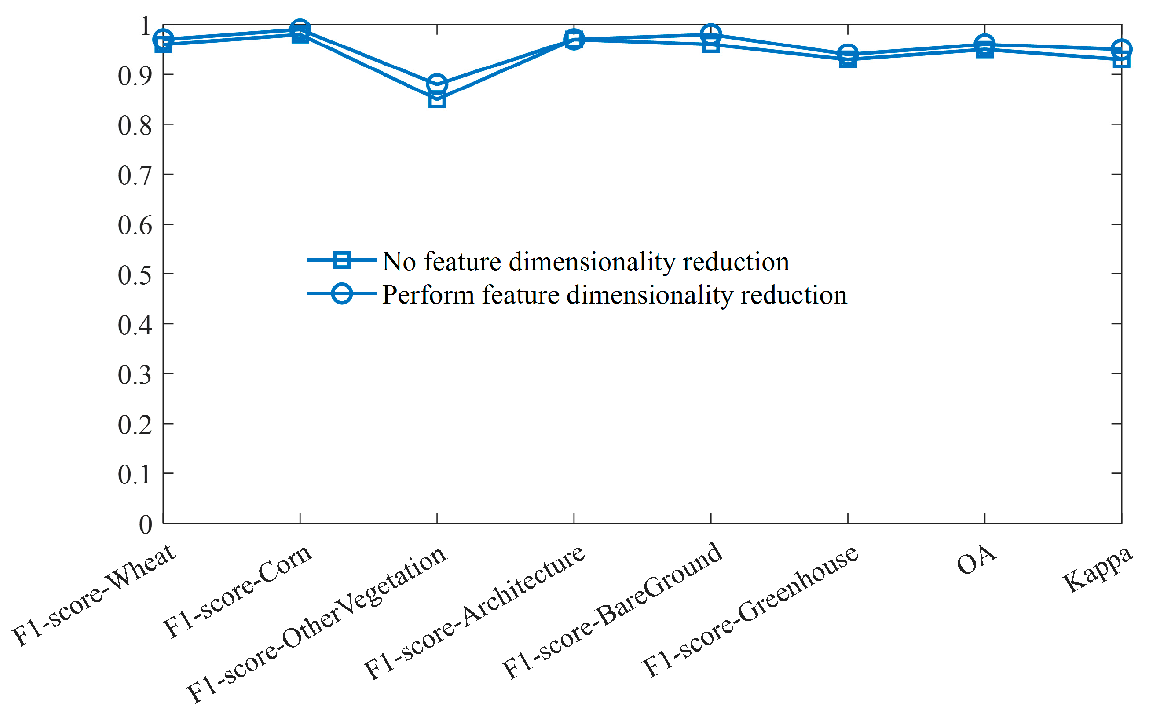
The fusion model proposed in this paper was trained using the aforementioned training samples. The training was conducted under two scenarios: with characteristic dimensionality reduction, and without characteristic dimensionality reduction. Additionally, 10% of all samples were randomly selected as a test set, to evaluate the classification accuracy. The results are presented in Figure 12. It can be observed that the model with characteristic dimensionality reduction exhibits an improved classification accuracy, compared to the model without dimensionality reduction. Specifically, the OA and kappa coefficient increase by 1 percentage point and 0.03, respectively. Hence, it can be concluded that performing dimensionality reduction on high-dimensional characteristics before classification helps to alleviate the degradation in the model performance caused by the Hughes phenomenon.

4.4. Extraction of Crop Area in the Entire Region

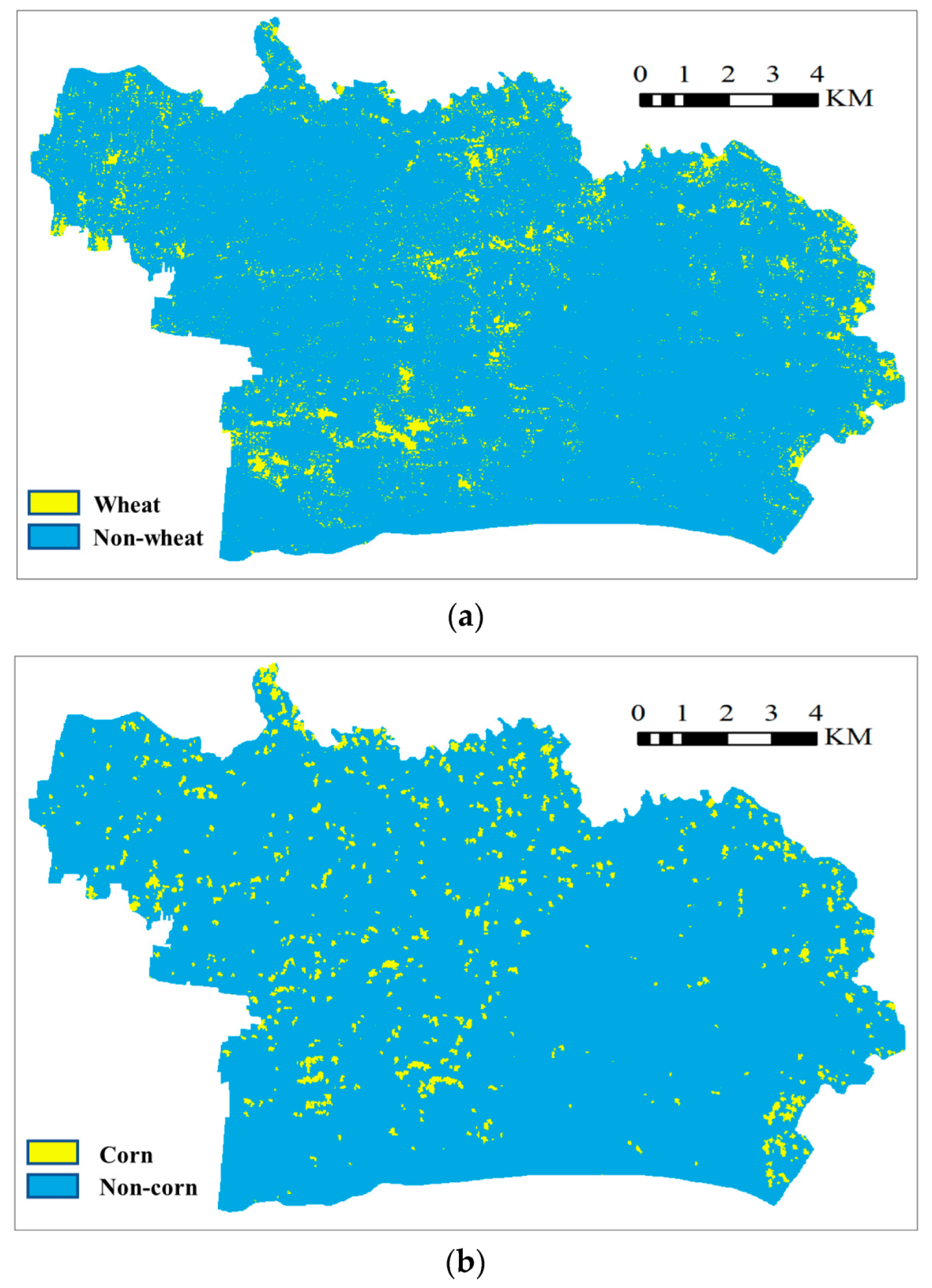
The model was trained using sample data from regions A and B. The area of the main crops was extracted from the entire study area. The planting distribution of wheat and corn in Yangling District is shown in Figure 13a,b. It can be observed that wheat is primarily distributed in the northwest and northeast regions of Yangling District, as well as in the central area that spans from north to south. On the other hand, the distribution of corn shows a relatively uniform pattern.
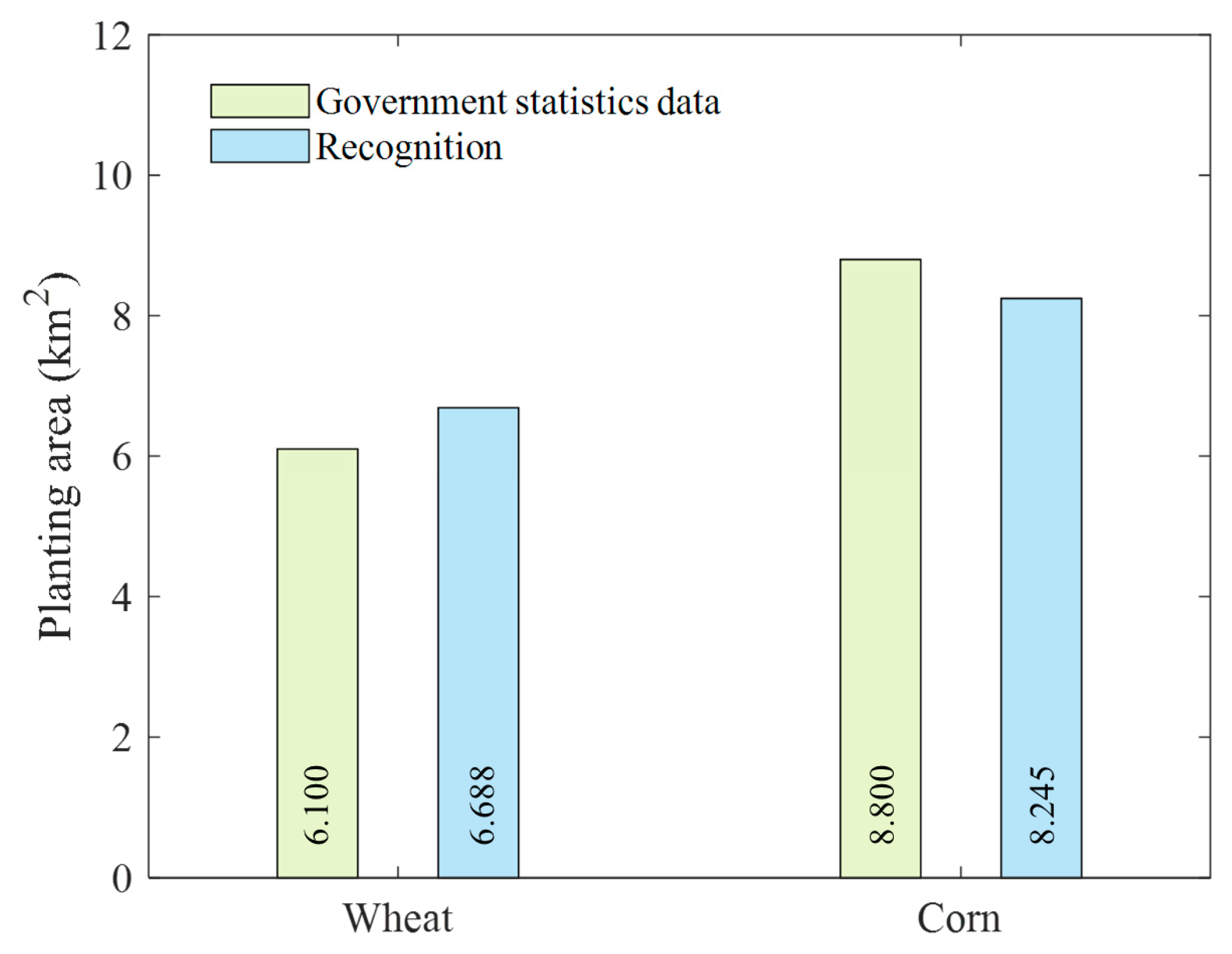
According to publicly available data from the Shaanxi Provincial Bureau of Statistics, the planting areas of wheat and corn in Yangling District for the year 2021 have been obtained. Figure 14 illustrates a comparison between the government’s statistical data, and the planting areas extracted in this paper. The results indicate that there is a discrepancy between the extracted area and the official statistics. However, this discrepancy only accounts for 9.6% and 6.3% of the total planting area, respectively. One possible explanation for this discrepancy could be the variations in planting conditions caused by the differences in the data collection time and the satellite imagery acquisition time. Additionally, it should be noted that some errors might exist in the statistical yearbook data. Hence, the extracted area could, to some extent, reflect the actual crop-planting situation.

5. Discussion

In the classification experiments on the entire images of Region A and Region B, it can be observed that traditional ML classification methods often exhibit a lower accuracy due to significant class confusion in the classification results. This may be attributed to the relatively insufficient feature learning capabilities of traditional ML methods, compared to DL methods with complex network structures [51,52]. Another aspect worth discussing is the model’s adaptability in classifying new data, which is also an important criterion in evaluating the model. In experiments where the training samples do not belong to the classified regions, the proposed model demonstrates a higher adaptability, compared to other methods. This can be attributed to the strong feature learning capability of the CNN classification network employed in the proposed model. This part of the network leverages three branches, with different convolutional layers, to learn features more comprehensively. Moreover, the introduced batch normalization operation enables the network to continuously adapt to new data distributions. Therefore, this method could serve as a valuable reference for other ground-information extraction tasks.
Although the effectiveness of this method has been well validated in the crop area extraction experiments in Yangling, further research is needed concerning the crop-area extraction on a larger scale. For larger-scale crop-area extraction tasks, the strategy for selecting training samples may need to be adjusted slightly. It is important to avoid the excessive concentration of samples during selection, to maintain their representativeness. Additionally, the extraction of crop areas on a larger scale is subject to constraints imposed by weather conditions, making it challenging to obtain cloud-free optical images for the entire region. Therefore, it is necessary to consider integrating optical and SAR images in future research, to mitigate the effects of weather. Furthermore, different types of ground cover should be taken into account in large-scale scenarios; for instance, when dealing with areas that include bodies of water, such as lakes, a mask operation could be performed prior to crop classification recognition.

6. Conclusions

In this research paper, a novel approach called the FSACNN was proposed, specifically for the task of extracting the crop-planting areas from high-dimensional characteristic input classification patterns. The method combines data dimensionality reduction and classification techniques, to optimize the extraction results. The performance of the FSACNN was evaluated using a multi-temporal hyperspectral remote sensing dataset from the Yangling Agricultural Demonstration Zone, and it was compared with other methods. The results of the study indicate that the FSACNN method outperforms the compared methods, achieving a superior extraction effect for crop-planting areas. Moreover, the method demonstrates a strong robustness when predicting new data, which has implications for other tasks involving surface-information extraction. Comparisons with statistical data on crops in the Yangling District demonstrate that the extracted crop-planting areas reflect the actual planting situation, to a certain extent. It is worth mentioning that the data used in this study came exclusively from optical satellites. The next focus of the research will be how to apply the FSACNN method to other types of satellite data.

Author Contributions

Data curation, J.G.; methodology, X.K., J.G. and J.B.; project administration, J.G.; software, X.K.; supervision, J.G.; validation, X.K.; writing original draft, X.K.; writing review and editing, X.K., J.G., J.B., H.G. and H.W. All authors have read and agreed to the published version of the manuscript.

Funding

This work was supported by the National Natural Science Foundation of China (grant No. U22B2015 and 41301450).

Data Availability Statement

The data presented in this study are openly available in Science Data Bank at 10.57760/sciencedb.09665.

Conflicts of Interest

The authors declare no conflict of interest.

References

  1. Lee, M.-K.; Golzarian, M.R.; Kim, I. A new color index for vegetation segmentation and classification. Precis. Agric. 2021, 22, 179–204. [Google Scholar] [CrossRef]
  2. Qiu, B.; Jiang, F.; Chen, C.; Tang, Z.; Wu, W.; Berry, J. Phenology-pigment based automated peanut mapping using sentinel-2 images. GIScience Remote Sens. 2021, 58, 1335–1351. [Google Scholar] [CrossRef]
  3. Bongiovanni, R.; Lowenberg-DeBoer, J. Precision agriculture and sustainability. Precis. Agric. 2004, 5, 359–387. [Google Scholar] [CrossRef]
  4. Tian, Y.; Yang, C.; Huang, W.; Tang, J.; Li, X.; Zhang, Q. Machine learning-based crop recognition from aerial remote sensing imagery. Front. Earth Sci. 2021, 15, 54–69. [Google Scholar] [CrossRef]
  5. Chen, B.; Zheng, H.; Wang, L.; Hellwich, O.; Chen, C.; Yang, L.; Liu, T.; Luo, G.; Bao, A.; Chen, X. A joint learning Im-BiLSTM model for incomplete time-series Sentinel-2A data imputation and crop classification. Int. J. Appl. Earth Obs. Geoinf. 2022, 108, 102762. [Google Scholar] [CrossRef]
  6. Yan, S.; Yao, X.; Zhu, D.; Liu, D.; Zhang, L.; Yu, G.; Gao, B.; Yang, J.; Yun, W. Large-scale crop mapping from multi-source optical satellite imageries using machine learning with discrete grids. Int. J. Appl. Earth Obs. Geoinf. 2021, 103, 102485. [Google Scholar] [CrossRef]
  7. Yuan, Y.; Lin, L.; Liu, Q.; Hang, R.; Zhou, Z.-G. SITS-Former: A pre-trained spatio-spectral-temporal representation model for Sentinel-2 time series classification. Int. J. Appl. Earth Obs. Geoinf. 2022, 106, 102651. [Google Scholar] [CrossRef]
  8. Amorim, M.T.A.; Silvero, N.E.; Bellinaso, H.; Gómez, A.M.R.; Greschuk, L.T.; Campos, L.R.; Demattê, J.A. Impact of soil types on sugarcane development monitored over time by remote sensing. Precis. Agric. 2022, 23, 1532–1552. [Google Scholar] [CrossRef]
  9. Martinez, J.A.C.; La Rosa, L.E.C.; Feitosa, R.Q.; Sanches, I.D.A.; Happ, P.N. Fully convolutional recurrent networks for multidate crop recognition from multitemporal image sequences. ISPRS J. Photogramm. Remote Sens. 2021, 171, 188–201. [Google Scholar] [CrossRef]
  10. Zhou, Y.n.; Luo, J.; Feng, L.; Yang, Y.; Chen, Y.; Wu, W. Long-short-term-memory-based crop classification using high-resolution optical images and multi-temporal SAR data. GIScience Remote Sens. 2019, 56, 1170–1191. [Google Scholar] [CrossRef]
  11. Wang, Y.; Feng, L.; Sun, W.; Zhang, Z.; Zhang, H.; Yang, G.; Meng, X. Exploring the potential of multi-source unsupervised domain adaptation in crop mapping using Sentinel-2 images. GIScience Remote Sens. 2022, 59, 2247–2265. [Google Scholar] [CrossRef]
  12. Adrian, J.; Sagan, V.; Maimaitijiang, M. Sentinel SAR-optical fusion for crop type mapping using deep learning and Google Earth Engine. ISPRS J. Photogramm. Remote Sens. 2021, 175, 215–235. [Google Scholar] [CrossRef]
  13. Jayakumari, R.; Nidamanuri, R.R.; Ramiya, A.M. Object-level classification of vegetable crops in 3D LiDAR point cloud using deep learning convolutional neural networks. Precis. Agric. 2021, 22, 1617–1633. [Google Scholar] [CrossRef]
  14. Zhao, S.; Liu, X.; Ding, C.; Liu, S.; Wu, C.; Wu, L. Mapping rice paddies in complex landscapes with convolutional neural networks and phenological metrics. GIScience Remote Sens. 2020, 57, 37–48. [Google Scholar] [CrossRef]
  15. Elango, S.; Haldar, D.; Danodia, A. Discrimination of maize crop in a mixed Kharif crop scenario with synergism of multiparametric SAR and optical data. Geocarto Int. 2022, 37, 5307–5326. [Google Scholar] [CrossRef]
  16. Duro, D.C.; Franklin, S.E.; Dubé, M.G. A comparison of pixel-based and object-based image analysis with selected machine learning algorithms for the classification of agricultural landscapes using SPOT-5 HRG imagery. Remote Sens. Environ. 2012, 118, 259–272. [Google Scholar] [CrossRef]
  17. Gumma, M.K.; Thenkabail, P.S.; Teluguntla, P.G.; Oliphant, A.; Xiong, J.; Giri, C.; Pyla, V.; Dixit, S.; Whitbread, A.M. Agricultural cropland extent and areas of South Asia derived using Landsat satellite 30-m time-series big-data using random forest machine learning algorithms on the Google Earth Engine cloud. GIScience Remote Sens. 2020, 57, 302–322. [Google Scholar] [CrossRef] [Green Version]
  18. Wang, Z.; Zhao, Z.; Yin, C. Fine crop classification based on UAV hyperspectral images and random forest. ISPRS Int. J. Geo-Inf. 2022, 11, 252. [Google Scholar] [CrossRef]
  19. Maponya, M.G.; Van Niekerk, A.; Mashimbye, Z.E. Pre-harvest classification of crop types using a Sentinel-2 time-series and machine learning. Comput. Electron. Agric. 2020, 169, 105164. [Google Scholar] [CrossRef]
  20. Löw, F.; Conrad, C.; Michel, U. Decision fusion and non-parametric classifiers for land use mapping using multi-temporal RapidEye data. ISPRS J. Photogramm. Remote Sens. 2015, 108, 191–204. [Google Scholar] [CrossRef]
  21. Kwak, G.-H.; Park, C.-W.; Lee, K.-D.; Na, S.-I.; Ahn, H.-Y.; Park, N.-W. Potential of hybrid CNN-RF model for early crop mapping with limited input data. Remote Sens. 2021, 13, 1629. [Google Scholar] [CrossRef]
  22. Yuan, Y.; Lin, L.; Zhou, Z.-G.; Jiang, H.; Liu, Q. Bridging optical and SAR satellite image time series via contrastive feature extraction for crop classification. ISPRS J. Photogramm. Remote Sens. 2023, 195, 222–232. [Google Scholar] [CrossRef]
  23. Ji, S.; Zhang, C.; Xu, A.; Shi, Y.; Duan, Y. 3D convolutional neural networks for crop classification with multi-temporal remote sensing images. Remote Sens. 2018, 10, 75. [Google Scholar] [CrossRef] [Green Version]
  24. Moreno-Revelo, M.Y.; Guachi-Guachi, L.; Gómez-Mendoza, J.B.; Revelo-Fuelagán, J.; Peluffo-Ordóñez, D.H. Enhanced convolutional-neural-network architecture for crop classification. Appl. Sci. 2021, 11, 4292. [Google Scholar] [CrossRef]
  25. Seydi, S.T.; Amani, M.; Ghorbanian, A. A dual attention convolutional neural network for crop classification using time-series Sentinel-2 imagery. Remote Sens. 2022, 14, 498. [Google Scholar] [CrossRef]
  26. Sun, H.; Zheng, X.; Lu, X. A supervised segmentation network for hyperspectral image classification. IEEE Trans. Image Process. 2021, 30, 2810–2825. [Google Scholar] [CrossRef]
  27. Yang, W.; Nigon, T.; Hao, Z.; Paiao, G.D.; Fernández, F.G.; Mulla, D.; Yang, C. Estimation of corn yield based on hyperspectral imagery and convolutional neural network. Comput. Electron. Agric. 2021, 184, 106092. [Google Scholar] [CrossRef]
  28. Li, B.; Wang, K.C.; Zhang, A.; Yang, E.; Wang, G. Automatic classification of pavement crack using deep convolutional neural network. Int. J. Pavement Eng. 2020, 21, 457–463. [Google Scholar] [CrossRef]
  29. Saleem, M.H.; Potgieter, J.; Arif, K.M. Automation in agriculture by machine and deep learning techniques: A review of recent developments. Precis. Agric. 2021, 22, 2053–2091. [Google Scholar] [CrossRef]
  30. Hu, W.; Huang, Y.; Wei, L.; Zhang, F.; Li, H. Deep convolutional neural networks for hyperspectral image classification. J. Sens. 2015, 2015, 258619. [Google Scholar] [CrossRef] [Green Version]
  31. Liao, C.; Wang, J.; Xie, Q.; Baz, A.A.; Huang, X.; Shang, J.; He, Y. Synergistic use of multi-temporal RADARSAT-2 and VENµS data for crop classification based on 1D convolutional neural network. Remote Sens. 2020, 12, 832. [Google Scholar] [CrossRef] [Green Version]
  32. Zhang, H.; Liu, W.; Zhang, L. Seamless and automated rapeseed mapping for large cloudy regions using time-series optical satellite imagery. ISPRS J. Photogramm. Remote Sens. 2022, 184, 45–62. [Google Scholar] [CrossRef]
  33. Ji, S.; Zhang, Z.; Zhang, C.; Wei, S.; Lu, M.; Duan, Y. Learning discriminative spatiotemporal features for precise crop classification from multi-temporal satellite images. Int. J. Remote Sens. 2020, 41, 3162–3174. [Google Scholar] [CrossRef]
  34. Zhu, J.; Pan, Z.; Wang, H.; Huang, P.; Sun, J.; Qin, F.; Liu, Z. An improved multi-temporal and multi-feature tea plantation identification method using Sentinel-2 imagery. Sensors 2019, 19, 2087. [Google Scholar] [CrossRef] [PubMed] [Green Version]
  35. Yang, S.; Gu, L.; Li, X.; Jiang, T.; Ren, R. Crop classification method based on optimal feature selection and hybrid CNN-RF networks for multi-temporal remote sensing imagery. Remote Sens. 2020, 12, 3119. [Google Scholar] [CrossRef]
  36. Kyere, I.; Astor, T.; Graß, R.; Wachendorf, M. Agricultural crop discrimination in a heterogeneous low-mountain range region based on multi-temporal and multi-sensor satellite data. Comput. Electron. Agric. 2020, 179, 105864. [Google Scholar] [CrossRef]
  37. Zhang, H.; Yuan, H.; Du, W.; Lyu, X. Crop Identification Based on Multi-Temporal Active and Passive Remote Sensing Images. ISPRS Int. J. Geo-Inf. 2022, 11, 388. [Google Scholar] [CrossRef]
  38. Hughes, G. On the mean accuracy of statistical pattern recognizers. IEEE Trans. Inf. Theory 1968, 14, 55–63. [Google Scholar] [CrossRef] [Green Version]
  39. Hinton, G.E.; Salakhutdinov, R.R. Reducing the dimensionality of data with neural networks. Science 2006, 313, 504–507. [Google Scholar] [CrossRef] [Green Version]
  40. Yu, M.; Quan, T.; Peng, Q.; Yu, X.; Liu, L. A model-based collaborate filtering algorithm based on stacked AutoEncoder. Neural Comput. Appl. 2022, 34, 2503–2511. [Google Scholar] [CrossRef]
  41. Liu, Y.; Chen, X.; Wang, Z.; Wang, Z.J.; Ward, R.K.; Wang, X. Deep learning for pixel-level image fusion: Recent advances and future prospects. Inf. Fusion 2018, 42, 158–173. [Google Scholar] [CrossRef]
  42. Lv, Z.; Qiao, L.; Li, J.; Song, H. Deep-learning-enabled security issues in the internet of things. IEEE Internet Things J. 2020, 8, 9531–9538. [Google Scholar] [CrossRef]
  43. Chen, L.; Letu, H.; Fan, M.; Shang, H.; Tao, J.; Wu, L.; Zhang, Y.; Yu, C.; Gu, J.; Zhang, N. An Introduction to the Chinese High-Resolution Earth Observation System: Gaofen-1~7 Civilian Satellites. J. Remote Sens. 2022, 2022, 9769536. [Google Scholar] [CrossRef]
  44. Shi, L.; Huang, X.; Zhong, T.; Taubenböck, H. Mapping plastic greenhouses using spectral metrics derived from GaoFen-2 satellite data. IEEE J. Sel. Top. Appl. Earth Obs. Remote Sens. 2019, 13, 49–59. [Google Scholar] [CrossRef]
  45. Tong, X.; Zhao, W.; Xing, J.; Fu, W. Status and development of China high-resolution earth observation system and application. In Proceedings of the 2016 IEEE International Geoscience and Remote Sensing Symposium (IGARSS), Beijing, China, 10–15 July 2016; pp. 3738–3741. [Google Scholar]
  46. Haralick, R.M.; Shanmugam, K.; Dinstein, I.H. Textural features for image classification. In IEEE Transactions on Systems, Man, and Cybernetics; IEEE: New York, NY, USA, 1973; pp. 610–621. [Google Scholar]
  47. Tian, F.; Fensholt, R.; Verbesselt, J.; Grogan, K.; Horion, S.; Wang, Y. Evaluating temporal consistency of long-term global NDVI datasets for trend analysis. Remote Sens. Environ. 2015, 163, 326–340. [Google Scholar] [CrossRef]
  48. Yan, K.; Gao, S.; Chi, H.; Qi, J.; Song, W.; Tong, Y.; Mu, X.; Yan, G. Evaluation of the vegetation-index-based dimidiate pixel model for fractional vegetation cover estimation. IEEE Trans. Geosci. Remote Sens. 2021, 60, 21382349. [Google Scholar] [CrossRef]
  49. Chollet, F. Xception: Deep learning with depthwise separable convolutions. In Proceedings of the IEEE Conference on Computer Vision and Pattern Recognition, Honolulu, HI, USA, 21–26 July 2017; pp. 1251–1258. [Google Scholar]
  50. Fang, P.; Zhang, X.; Wei, P.; Wang, Y.; Zhang, H.; Liu, F.; Zhao, J. The classification performance and mechanism of machine learning algorithms in winter wheat mapping using Sentinel-2 10 m resolution imagery. Appl. Sci. 2020, 10, 5075. [Google Scholar] [CrossRef]
  51. LeCun, Y.; Bengio, Y.; Hinton, G. Deep learning. Nature 2015, 521, 436–444. [Google Scholar] [CrossRef]
  52. Silver, D.; Huang, A.; Maddison, C.J.; Guez, A.; Sifre, L.; Van Den Driessche, G.; Schrittwieser, J.; Antonoglou, I.; Panneershelvam, V.; Lanctot, M. Mastering the game of Go with deep neural networks and tree search. Nature 2016, 529, 484–489. [Google Scholar] [CrossRef] [PubMed]
Figure 1. Study area.
Remotesensing 15 03792 g001
Figure 2. Composite RGB image.
Remotesensing 15 03792 g002
Figure 3. Ground truth of the training sample area.
Remotesensing 15 03792 g003
Figure 4. Flow chart of the process of extracting the crop-planting area.
Remotesensing 15 03792 g004
Figure 5. Structure of the autoencoder.
Remotesensing 15 03792 g005
Figure 6. Structure of the stacked autoencoder.
Remotesensing 15 03792 g006
Figure 7. Structure of the FSACNN.
Remotesensing 15 03792 g007
Figure 8. Classification results for each method for area A under condition 1. (a) DT. (b) RF. (c) SVM. (d) HICCNN. (e) CSCNN. (f) FSACNN. (g) Satellite imagery.
Remotesensing 15 03792 g008
Figure 9. Classification results for each method for area B under condition 1. (a) DT. (b) RF. (c) SVM. (d) HICCNN. (e) CSCNN. (f) FSACNN. (g) Satellite imagery.
Remotesensing 15 03792 g009
Figure 10. Classification results for each method under condition 2. (a) DT. (b) RF. (c) SVM. (d) HICCNN. (e) CSCNN. (f) FSACNN. (g) Satellite imagery.
Remotesensing 15 03792 g010
Figure 11. Standard deviation of the various characteristics. (a) Wheat. (b) Corn. (c) Other vegetation. (d) Urban. (e) Bare ground. (f) Greenhouse. (g) All classes.
Remotesensing 15 03792 g011aRemotesensing 15 03792 g011b
Figure 12. Classification accuracy before and after characteristic dimensionality reduction.
Remotesensing 15 03792 g012
Figure 13. Distribution of the main crops in Yangling District. (a) Wheat. (b) Corn.
Remotesensing 15 03792 g013
Figure 14. Planting area of the main crops.
Remotesensing 15 03792 g014
Table 1. The data acquisition dates and basic information of the main crops in the experimental area.
SatelliteSpatial
Resolution/m
BandAcquisition Date
GF-12Panchromatic18 May 2021
8Multispectral
GF-20.8Panchromatic4 May 2021
4Multispectral
GF-62Panchromatic14 April 2021
8Multispectral
Table 2. All characteristics used in this paper.
Feature NameIdentifier of Feature
GLCM texture (mean, variance, homogeneity, contrast, dissimilarity, entropy, angle second-order matrix, correlation) from GF-2Ft-1~Ft-8
Multispectral features (red, green, blue, near-infrared) from GF-2Ft-9~Ft-12
Multispectral features (red, green, blue, near-infrared) from GF-1Ft-13~Ft-16
Multispectral features (red, green, blue, near-infrared) from GF-6Ft-17~Ft-20
NDVI, RVI, ARI2 from GF-2Ft-21~Ft-23
NDVI, RVI, ARI2 from GF-1Ft-24~Ft-26
NDVI, RVI, ARI2 from GF-6Ft-27~Ft-29
Table 3. Classification accuracy of each method for area A under condition 1.
MethodF1-ScoreOA
(%)
Kappa
WheatCornOther VegetationUrbanBare GroundGreenhouse
DT0.920.950.740.910.950.8990.620.83
RF0.940.980.790.940.990.9593.880.88
SVM0.940.970.790.910.970.8892.890.87
HICCNN0.980.990.920.980.970.9697.360.95
CSCNN0.990.980.940.980.980.9697.470.96
FSACNN0.990.990.950.980.990.9898.570.97
Table 4. Classification accuracy of each method for area B under condition 1.
MethodF1-ScoreOA
(%)
Kappa
WheatCornOther VegetationUrbanBare GroundGreenhouse
DT0.890.830.760.940.890.7888.040.74
RF0.930.920.790.970.940.9492.020.80
SVM0.930.930.790.960.890.7691.230.79
HICCNN0.960.990.860.980.960.9895.260.88
CSCNN0.980.980.920.960.960.9795.880.92
FSACNN0.980.980.940.980.960.9797.760.94
Table 5. Classification accuracy of each method for area B under condition 2.
MethodF1-ScoreOA
(%)
Kappa
WheatCornOther VegetationUrbanBare GroundGreenhouse
DT0.860.730.340.660.740.7272.920.62
RF0.900.750.510.800.880.6678.520.71
SVM0.920.770.590.400.770.5378.060.70
HICCNN0.910.820.500.730.790.6979.010.72
CSCNN0.880.900.550.790.890.7183.260.79
FSACNN0.970.870.570.800.880.7587.150.83
Disclaimer/Publisher’s Note: The statements, opinions and data contained in all publications are solely those of the individual author(s) and contributor(s) and not of MDPI and/or the editor(s). MDPI and/or the editor(s) disclaim responsibility for any injury to people or property resulting from any ideas, methods, instructions or products referred to in the content.