A Two-Stage Track-before-Detect Method for Non-Cooperative Bistatic Radar Based on Deep Learning

Abstract

Compared with traditional active detection radar, non-cooperative bistatic radar has a series of advantages, such as a low cost and low detectability. However, in real-life scenarios, it is limited by the non-cooperation of the radiation source and the bistatic geometric model, resulting in a low target signal-to-noise ratio (SNR) and unstable detection between frames in the radar scanning cycle. The traditional detect-before-track (DBT) method fails to exploit adequately the target information and is incapable of achieving consistent and effective tracking. Therefore, in this paper, we propose a two-stage track-before-detect (TBD) method based on deep learning. This method employs a low-threshold detection network to identify the target initially, followed by utilizing the model method to ascertain potential tracks. Subsequently, a diverse range of network structures are employed to extract and integrate position information, innovation score, and target structural information from the track in order to obtain the target track. Experimental results demonstrate the method’s ability to achieve multi-target tracking in highly cluttered environments, where the higher the number of frames processed, the better the target tracking effect. Moreover, the method exhibits real-time processing capabilities. Hence, this method provides an effective solution for target tracking in non-cooperative bistatic radar systems.

1. Introduction

With the increasing complexity of the electromagnetic environment in the modern battlefield, traditional active radar is often easily discovered by the enemy because of its active emission of electromagnetic waves. This has led to the study of a new radar system, namely non-cooperative bistatic radar systems. A non-cooperative radar emitter target detection system is a passive detection system based on the bistatic radar working mode, which uses non-cooperative radar as the radiation source [1]. Compared with the traditional active monostatic radar, non-cooperative bistatic radar has obvious advantages, such as low detectability, low cost, and strong ‘four anti’ abilities [2]. The working principle of the receiving system is to detect and analyze direct wave signals from the target scattering echo signal by taking the signal emitted by the non-cooperative radar emitter as the reference to realize target positioning and tracking [3]. However, in practical applications, the lack of cooperation from the radiation source introduces synchronization errors and parameter estimation errors in direct wave signals. Moreover, the unique geometric model of cooperative bistatic radar leads to significant direct wave and direct wave multipath interference in the echo channel. Consequently, non-cooperative bistatic radar systems suffer from reduced space and time synchronization accuracy. The target positioning accuracy and the echo signal-to-noise ratio (SNR) are low, and target detection between frames is unstable, which increases the difficulty of subsequent tracking [4].

The simplest approach to enhance the detection performance of a system in low signal-to-noise ratio (SNR) conditions is by reducing the detection threshold. However, blindly reducing the detection threshold will introduce clutter and generate a large number of false alarms. In this case, using the traditional detect-before-track (DBT) method will produce many false tracks; therefore, the track-before-detect (TBD) method was proposed. The difference between the TBD and the traditional DBT lies in the fact that the TBD does not perform threshold detection processing or set a lower threshold in a single frame. The radar echo data information is digitized and stored. After multi-frame data processing, the detection result is generated, and the target track is estimated at the same time [5]. TBD avoids threshold detection and retains the original measurement of the target. The SNR is enhanced by collecting multiple frames, which can significantly improve the tracking accuracy [6]. Some scholars have carried out research on the TBD method for bistatic/multistatic radar based on civil radiation sources [7,8,9,10]. In reference [7], an orthogonal frequency division multiplexing signal was used as the radiation source, and the TBD method was used to recursively estimate the target existence probability and state the probability density of each range-Doppler unit to realize multi-target tracking. Reference [8] used GNSS as the radiation source and combined it with various technical means, such as TBD and target motion compensation, to improve ship target detection. In reference [9], a Bayesian TBD method was used to detect and track small unmanned aerial vehicles (UAVs) using GSM passive radar. By preprocessing and reducing the dimensionality of the radar data, the complexity of the algorithm was reduced, and the efficiency of the target detection and tracking was improved. In reference [10], a novel TBD method was proposed using AM broadcast signals as the radiation source. A constant velocity equation and an initial position equation were created, and the method was compared with several TBD methods. However, there is currently little research focused on how to perform TBD when using radar signals as non-cooperative radiation sources. Additionally, when the observation space has a large number of false alarms, existing methods often encounter challenges such as excessive calculations and poor detection performance. The commonly adopted non-coherent accumulation method mainly takes into account the amplitude, square amplitude, or likelihood ratio between the target power and clutter, while ignoring the use of other multi-dimensional information. For example, the smoothness of a real track is usually better than that of a false track, and if this information is considered, a large number of false alarms can be handled more effectively. However, using mathematical derivations alone to obtain an expression of this detector is difficult.

With the continual development of deep learning, neural networks have been widely used in many fields due to their strong nonlinear fitting ability. In recent years, some methods have been proposed to combine TBD with deep learning networks for weak target detection. For example, in reference [11,12], neural networks were used for preprocessing, followed by the TBD method for accumulating. However, these methods relied predominantly on deep learning techniques for data preprocessing and overlooked the multidimensional characteristics of the target. On the other hand, alternative approaches incorporated the TBD framework for intra-frame detection, as illustrated in studies [13,14]. However, these methods may not have adequately considered nonhomogeneous backgrounds. In order to address the issue of deep feature extraction, reference [15] introduced the DBU-MF-TBD method, which was based on the DBU-Net network structure. This particular method enhanced target detection by acquiring latent features and motion patterns through learning. Aiming to solve the problem of large amounts of data, reference [16] proposed a two-stage TBD method to alleviate the pressure of data processing. Motivated by these factors, this paper introduces a two-stage track-before-detect method for non-cooperative bistatic radar based on deep learning, using L-band shore-to-sea radar as the non-cooperative radiation source for experimental verification. Firstly, the method employs a low-threshold target detection network to perform single-frame detection on the data, aiming to reduce the data volume and relieve the pressure of subsequent data processing. Secondly, the potential track is determined by the model method, and the discrete observation data are transformed into track data with certain spatial and temporal correlations. Finally, a convolutional neural network and a recurrent neural network are used to extract the position information, innovation score, and target structure information from the track, thereby enabling the precise location and tracking of the target. Experimental results demonstrate that the proposed method achieves multi-target tracking even in the presence of clutter, with improved tracking performance as the number of processed frames increases. Additionally, the method exhibits a certain level of real-time processing capability.

2. Methods

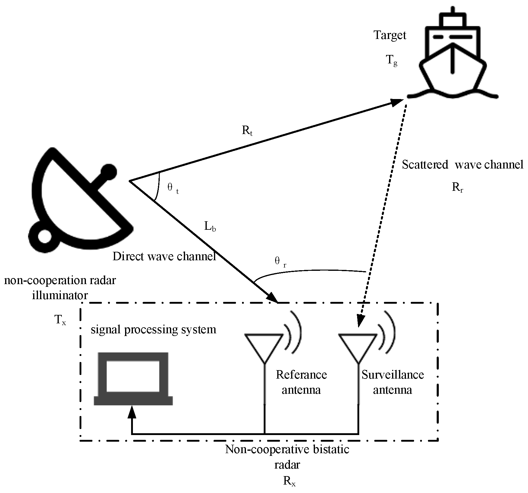
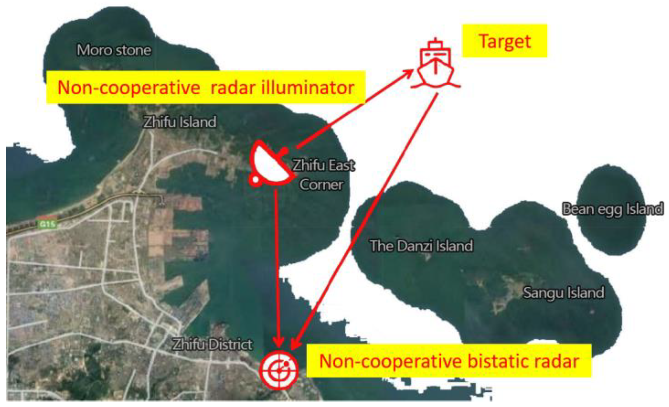
2.1. System Working Principle

The target detection principle of the non-cooperative bistatic radar system investigated in this study is shown in Figure 1. The non-cooperative radar radiation source used in the detection system is L-band shore-to-sea radar, and the detection targets are ships entering and leaving a port. Due to the non-cooperation of the radiation source, in order to synchronize the subsequent system, it is necessary to establish an additional reference channel to receive the direct wave signal of the non-cooperative radiation source. Therefore, the system has two channels: a direct wave channel and a scattering echo channel. Among them, the reference antenna of the direct wave channel usually receives side lobe signals from the non-cooperative radiation source, and the monitoring antenna of the scattering wave channel receives the scattering wave signal returned after the non-cooperative radiation source irradiates the target. Finally, the signal processing system processes the data received by the direct wave and the scattering wave channel to complete the target positioning and tracking. In Figure 1, $T_x$ is the non-cooperative radar emitter, $R_x$ is the non-cooperative bistatic radar, $T_g$ is the target, the baseline distance $L_b$ is the distance between $T_x$ and $R_x$, and ${\theta }_t$ and ${\theta }_r$ are the target azimuths of the emitter and the non-cooperative bistatic radar, respectively. $R_t$ and $R_r$ are the distances from the target to the emitter and the non-cooperative bistatic radar, respectively. The bistatic distance difference is $R_d=R_t+R_r-L_b$.

Figure 2 presents the signal processing flow chart of the non-cooperative bistatic radar system. The direct wave channel of the receiver in the figure executes direct wave signal extraction and reconstruction, time–frequency synchronization, and azimuth synchronization processing, while the other scattering echo channel executes pulse compression, direct wave interference suppression, and other detection processes. It obtains azimuths, bistatic distances, and Doppler information and, finally, displays an output on the display terminal [17].

2.2. Detection Performance Analysis

In non-cooperative bistatic radar, the purpose of detection processing is to identify the target and extract its bistatic distance, azimuth, and Doppler position. The original echo data can be divided into two dimensions: ‘slow’ time and ‘fast’ time. The ‘slow’ time represents the number of PRT sequences, and the ‘fast’ time represents the number of sampling points along a distance. Standard matched filtering of the echo signal in the ‘fast’ time dimension can be used to improve the resolution of the distance dimension and obtain a clearer contour. Its principle is the cross correlation between the echo signal and the reference signal [18]. Application of the fast Fourier transform (FFT) to multiple pulse trains in the ‘slow’ time domain can complete the Doppler processing, and a target with a stable speed will be concentrated in the Doppler domain. The detection involves finding the peak value of the threshold in the two-dimensional plane through CA-CFAR. However, this method performs poorly in non-cooperative bistatic radar systems with low SNR and unstable target signal detection. In order to understand this, the following analysis is carried out.

In general, the target and the receiver are not covered by the main lobe of the transmitter antenna at the same time. A direct wave often comes from the side lobe radiation of the radiation source, so detection of the direct wave from a non-cooperative radiation source is mostly via side lobe detection. The side lobe level of radar antenna is generally 20~50 dB lower than the peak of the main lobe. Compared with the direct wave, the target scattering echo is attenuated again due to reflection, and the power difference between the direct wave and the target scattering echo is very large. In order to quantify further the detection performance of non-cooperative bistatic radar, the bistatic radar range equation is particularly important:

$${(R_t{R}_r)}_{\max }=\sqrt{\frac{P_t{T}_c{G}_t{G}_r{\lambda }^2\sigma F_t{F}_r}{{(4\pi )}^{3}k{T}_s{B}_{n}SN{R}_{\min }{L}_t{L}_r}}$$

(1)

where $P_t$ is the emission power of the non-cooperative radiation source, $T_c$ is the single cumulative time; $G_t$ and $G_r$ are the power gains of the transmitting antenna and the receiver antenna, respectively; $\sigma$ is the radar cross section (RCS) of the target; $F_t$ and $F_r$ are the propagation shadows of transmitting and receiving antenna patterns, respectively; $k$ is the Boltzmann constant; $L_t$ and $L_r$ are the transmission loss and the total loss of the receiver, respectively; $T_s$ is the noise temperature of receiver system; $B_n$ is the bandwidth; and $SN{R}_{\min }$ is the minimum detectable SNR of the receiver.

The power density of the non-cooperative radar emitter to the detection target is calculated as follows [19]:

$$P_s=\frac{P_t{G}_t}{4\pi R_t^2}$$

(2)

Combining the specific radar parameters and the power density into Equation (1), the detection range equation based on non-cooperative bistatic radar can be further derived as

$$R_{r\max }=\sqrt{\frac{P_s{G}_r\sigma {\lambda }^2{T}_c}{{(4\pi )}^{2}k{T}_s{B}_{n}SN{R}_{\min }L}}$$

(3)

The parameters of the non-cooperative bistatic radar used in the field experiment are shown in

Table 1. Parameters of the non-cooperative bistatic radar.

Parameter	Sign	Unit	Value
Radiation source transmission power	$P_t$	kw	25
Target RCS	$\sigma$	m2	10
Receiver gain	$G_r$	dB	33
Frequency	$f_c$	MHz	1260
Bandwidth	$B_n$	MHz	3
System loss	$L$	dB	5

.

The data in Table 1 are substituted into Equation (3), and the distance from the non-cooperative radiation source to the target is set to 10 km. It can be calculated that when the target is 7.04 km away from the receiving station, the SNR is 5 dB. The target signal is weak and will decrease as the distance between the target and the receiving station increases. For example, when it is 10 km, the SNR will decrease to 1.95 dB. Therefore, for the detection of weak targets, setting a higher threshold will result in missed detections, and setting a lower threshold will result in a large number of false alarms. Considering the measured data as an example, Figure 3 show the PPI of two adjacent frames of non-cooperative bistatic radar. Target 1 and Target 2 have high energies in the first frame, while the energy in the latter frame is weak. The detection between frames of the radar scanning cycle is not stable, and the traditional DBT method is unable to produce a better performance.

2.3. Model Method to Determine the Potential Track

Track initiation establishes the target track quickly and efficiently before multi-target tracking and after data preprocessing, which is beneficial to reduce the data processing pressure of subsequent multi-target tracking [20]. Track initiation methods can be divided into two categories: sequential processing and batch processing. Sequential processing is suitable for track initiation in environments with relatively weak clutter. Representative methods are the intuitive method [21], the logic method [22], and its improved method [23]. Batch processing has a good track initiation performance in strong clutter environments, but the extent of the calculations is large. Representative methods are the Hough transform [24] and its improved method [25]. The number of false alarms in a single frame obtained by the target detection network in the subsequent experiments in this paper is approximately 25; thus, the number of false alarms is small, and the sequential processing method was selected for track initiation. Considering that the actual moving target potentially conforms to certain kinematic laws, we apply the following three constraint criteria in the track initiation process.

• Speed-based constraints. Let $r_i(i=1,2,\cdots ,N)$ be the position observation values obtained from $N$ consecutive scans, where $r_i$ corresponds to the center position of the detection box obtained by the target detection network. Now, consider two observations $r_i$ and $r_{i-1}$ from different frames, with the corresponding times $t_i$ and $t_{i-1}$, where $t_{i-1}<t_i$. Since the speeds of the ships in the experimental sea area are mostly 6~18 knots, the minimum speed is set as $V_{\min }=3m/s$, and the maximum speed is set as $V_{\max }=10m/s$, with the following specific constraints (4):

  $$V_{\min }\le \left|\frac{r_i-r_{i-1}}{t_i-t_{i-1}}\right|\le V_{\max }$$

  (4)
• Acceleration-based constraints. If the maximum acceleration is set to $a_{\max }$, then the distance between two adjacent observations at three different time points can be expressed as $r_i-r_{i-1}$, with specific constraints as Equation (5):

  $$\left|\frac{r_{i+1}-r_i}{t_{i+1}-t_i}-\frac{r_i-r_{i-1}}{t_i-t_{i-1}}\right|\le a_{\max }(t_{i+1}-t_i)$$

  (5)
• Angle-based constraints. The yaw angle refers to the alteration in the heading angle of a moving target from its pre-frame to post-frame position [26]. The heading transformation of the motion track lies within a certain range during the actual process of target motion. The specific limitations are as Equation (6):

  $$\arccos \left|\frac{(r_{i+1}-r_i)(r_i-r_{i-1})}{\left|r_{i+1}-r_i\right|\left|r_i-r_{i-1}\right|}\right|\le {\phi }_{\max }$$

  (6)

Based on the constraint conditions in Equations (4)–(6) and the low threshold settings of the target detection network, in order to initiate all the existing potential tracks to as great an extent as possible (especially the track of the weak target), this study uses the 3/8 logic method [27]. Once potential track initiation is complete, the subsequent prediction and correction are executed by the Singer model [28]. The specific track initiation steps can be divided into the following processes:

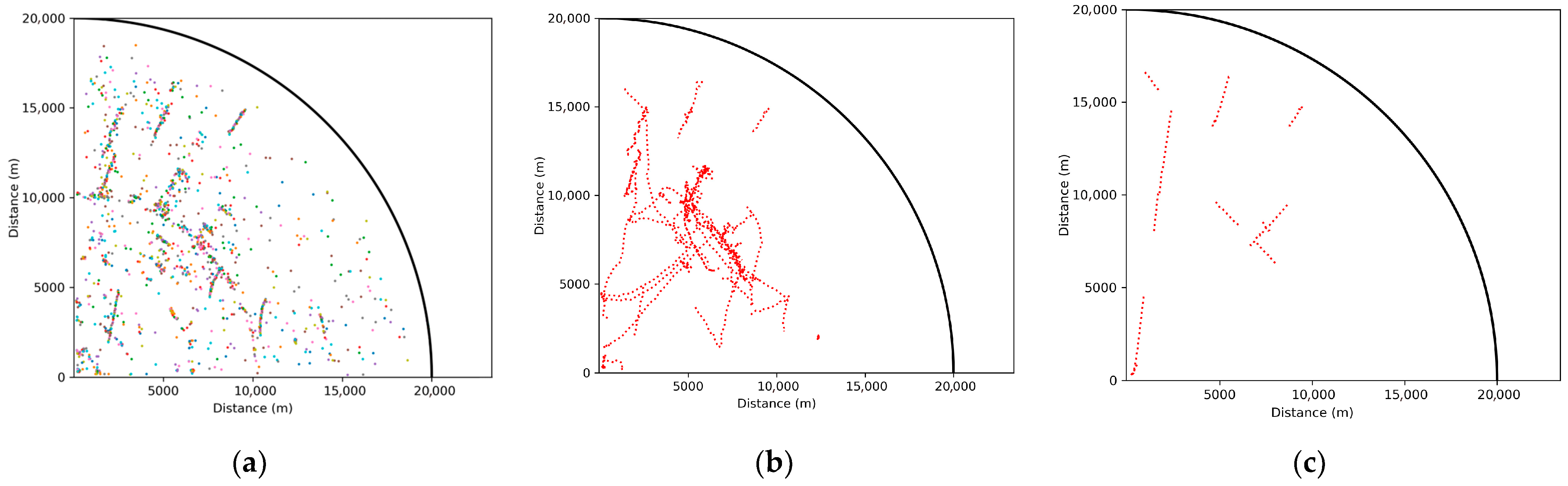
• The first frame of the plot is used to establish a temporary track, and then the initial correlation gate is established according to Equation (4). That is, if the observation value of the first frame has $N_1$ points and the observation value of the second frame has $N_2$ points, then the observation value of this scan will form a correlation matrix $D$, where the dimensions of the initial correlation matrix are $N_1\times N_2$. The observations in the correlation matrix that meet the speed constraints will be recorded.
• Tracks that satisfy velocity constraints undergo further checks for acceleration and angle constraints. If both conditions are met, the track is deemed transient. The relevant acceleration and angle information is then updated in preparation for the next match.
• If the subsequent gate has no observed value, the possible track is revoked. The above steps are repeated until a stable track is formed.
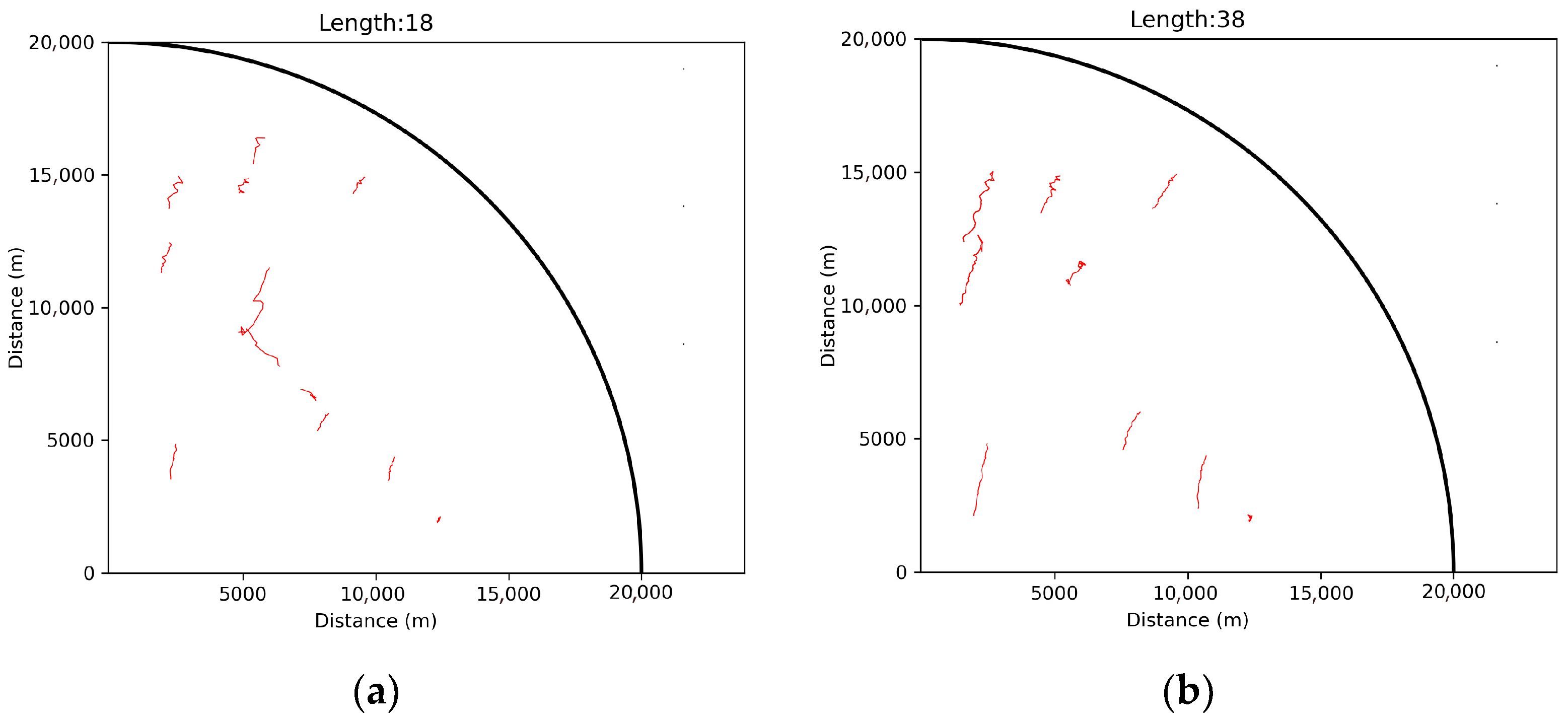
• All the potential tracks are traversed after initiation. If there are two points at the same position in the potential track, they can only be assigned to the same track for tracking. If they are mistakenly assigned to different tracks, it is necessary to compare the length of the two tracks, retain a longer track, or stitch the two tracks together.

This track initiating method is capable of processing observations that have yet to be associated with a known track, and it can either assign them to an existing track or create a new track. In track discrimination, two points at the same position can only be assigned to the same track for tracking. Therefore, this method is suitable for multi-target scenarios and can effectively handle multiple tracks. Using the Singer model to track a maneuvering target is described in the following:

• Filter initialization. The state transition matrix and the process noise covariance matrix are calculated by the given parameters: the target acceleration variance ${\sigma }_m^2$, the maximum acceleration probability $p_M$, the minimum acceleration probability $p_0$, the maximum acceleration $a_M$, and the maneuvering frequency $\alpha$ [29]. When the maneuvering acceleration is approximately uniformly distributed in $[-a_M,a_M]$, the variance ${\sigma }_m^2$ can be obtained by Equation (7):

  $${\sigma }_m^2=\frac{a_M^2}{3}(1+4p_M-p_0)$$

  (7)
• Data association. The Singer model is used to predict, and then the threshold is used to compare the predicted value with the actual observed value. The points within the threshold are selected, and the association probability is calculated.
• State update. Update the status of the chosen points whilst simultaneously updating the covariance matrix. The innovation score $\epsilon$ for the data association stage is calculated by Equation (8):

  $$\epsilon ={(Z_{k,l}-Z_{k|k-1,l})}^{⊺}{S}^{-1}{}_{k,l}(Z_{k,l}-Z_{k|k-1,l})$$

  (8)

  where $Z_{k,l}$ is the $l$-th observed value in the $k$-th frame, $Z_{k|k-1,l}$ represents the corresponding predicted value, $Z_{k,l}-Z_{k|k-1,l}$ is also called innovation in the Kalman filter and represents the error vector of the $l$-th observed value and its corresponding predicted value in the $k$-th frame, and $S^{-1}{}_{k,l}$ is the inverse operation of the innovation covariance matrix. The innovation score represents the difference between the current observation and the predicted value, as well as the influence of the observation noise. It is a quantitative index to evaluate the matching degree between the observation data and the predicted state. Some parameter settings used in the model method are shown in

  Table 2. Model method parameters.

  Parameter	Sign	Unit	Value
  Minimum initial velocity	$V_{\min }$	m/s	3
  Maximum initial velocity	$V_{\max }$	m/s	10
  Maximum initial acceleration	$a_{\max }$	m/s2	1
  Maximum initial heading angle	${\phi }_{\max }$	°	80
  Singer model maximum acceleration probability	$p_M$	%	5
  Singer model minimum acceleration probability	$p_0$	%	5
  Singer model minimum acceleration	$a_M^{}$	m/s2	0.5
  Singer model maneuver frequency	$\alpha$	s	8
  Tracking gate probability	$p_g$	%	99.97

  .

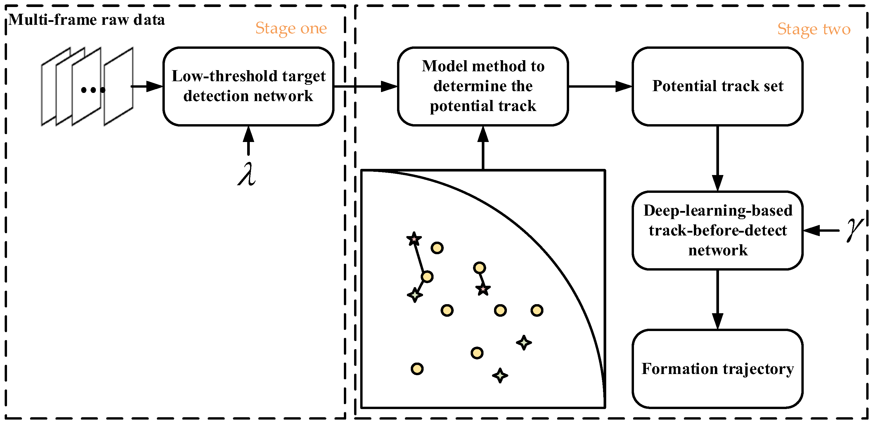
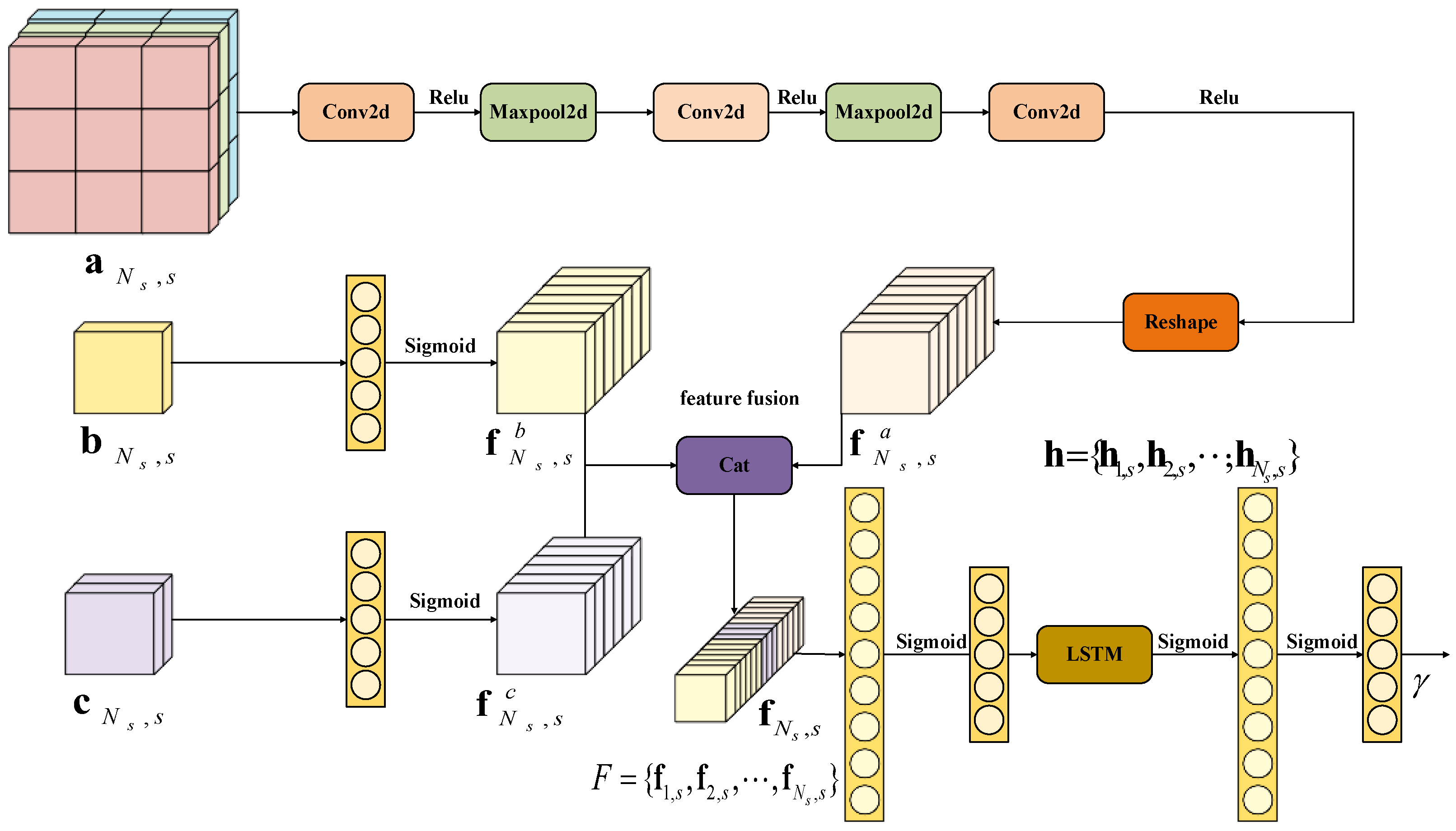
2.4. Two-Stage Track-before-Detect Method Based on Deep Learning

The traditional TBD method [30] usually uses coherent accumulation or non-coherent accumulation to achieve target tracking based on the prior model of motion. The choice of the prior motion model determines the tracking effect to a certain extent. If the real motion violates the assumed model, integration along the wrong path will lead to incorrect decisions. On the other hand, the computational cost associated with data processing is large, and other effective information from the observations is not used. Considering a track generated by the same target, the echo structure has a certain similarity between frames. Therefore, it is difficult to use traditional mathematical derivation to model the multi-dimensional features of the track, such as target structural information, position information, and innovation score predicted by the Singer model. With the continual development of deep learning, its powerful nonlinear mapping ability [31] and deep image feature extraction ability [32] have led to its wide used in various fields. This work aims to use the powerful fitting ability of neural networks to learn mapping relationships from multi-dimensional features to track confidence, thereby making a decision on the track. Here, the TBD method is actually regarded as a detector; that is, the first step is to use the target detection network to set a lower threshold, $\lambda$, to detect the target and reduce the quantity of data. The second step is to use the deep learning method to detect the track. The process is equivalent to using multi-dimensional features to determine whether a track is derived from the real target. If the frames are derived from the same real target, the confidence score of the track decision will be higher. If a track contains a false target, the confidence of the corresponding track decision will decrease due to the influence of multi-dimensional features. Figure 4 is the integral structure of the above process. The method of this paper is introduced in detail below.

Deep-Learning-Based Track-before-Detect Network

At present, there are many forms of neural networks. Feedforward neural networks (FNNs) are one of the common forms. They can approximate any continuous function and square integrable function with any precision [33]. Backpropagation neural networks are a representative of multi-layer feedforward neural networks [34]. For image processing problems and time series problems, scholars have proposed the use of convolutional neural networks (CNNs) and recurrent neural networks (RNNs), respectively. Convolutional neural networks can perform translation-invariant classification of input information through layer-by-layer convolutional blocks and have a certain representation learning ability [35]. Recurrent neural networks also connect the nodes between hidden layers, so they have a certain memory and are often used to learn the nonlinear features of sequences [36]. Long short-term memory (LSTM) is a typical recurrent neural network.

When designing the two-stage track-before-detect method for non-cooperative bistatic radar based on deep learning, the available features to consider include target location, innovation score, and target structure information. This paper proposes a track detection network that integrates convolution, a fully connected network, and LSTM, taking into account the different dimensions of the features and the unique processing capabilities of different networks. Its input consists of features with various attributes, and its output is the confidence that the track originates from a real target. Figure 5 shows the implementation of the network structure.

In order to distinguish it from the observation value $Z_{k,l}$ in each frame of radar scanning mentioned above, $s$ is marked as the order of the track, $N_s$ is marked as the number of observations of the track, and the observations are represented in lowercase letters. Therefore, observations in a track can be written as $\{z_{1,s},z_{2,s},z_{3,s},\cdots ,z_{N_s,s}\}$.

$a_{N_s,s}$ represents the radar PPI containing the target structure information, which is the result of the low-threshold detection of the target detection network. The sizes of the targets are not the same; thus, the dimensions of the detection results are also different. Here, the width and height of the input image are resized as $42\times 42$. For the real track generated by a target, although its echo energy will be affected by many factors, such as RCS fluctuation, its deep features should still have a certain correlation. Therefore, this study uses convolutional networks to extract the deep structural information of the target. $f_{N_s,s}^a$ is the one-dimensional feature vector obtained by $a_{N_s,s}$ after convolutional network extraction, which contains the structural information of the target. In the process of feature extraction, $f_{N_s,s}^a$ passes through three convolutional layers with a convolution kernel size of 3, in which a maximum pooling operation with a size of 2 is performed between two adjacent convolutional layers. This process is demonstrated in Equation (9), where $\ast$ represents the convolution operation; $W$ and $b$ represent the weight matrix and bias vector of each convolutional layer, respectively; ${\sigma }_r(\cdot )$r epresents the ReLU activation function; $\max (\cdot )$ represents maximum pooling; and $\mathrm{vec}(\cdot )$ represents flattening of the output of the convolutional layer into a one-dimensional vector.

$$\begin{array}{l}{f}_{N_s,s}^a=\mathrm{vec}({\sigma }_r(W_3\ast (\max ({\sigma }_r(W_2\ast (\max ({\sigma }_r(W_1\ast a_{N_s,s}+b_1)))+b_2)))+b_3))\\ \end{array}$$

(9)

In the Singer model tracking process, the variable $b_{N_s,s}$ is used to represent the difference between the current observation and the predicted value and the influence of the observation noise. In this model, $b_{N_s,s}$ represents the innovation score. The innovation score reflects the smoothness of the track. The track generated by the real target motion often conforms to kinematic rules. Therefore, the accuracy and validity of the innovation score are crucial, as they largely reflect the true condition of the target movement. It is worth noting that the innovation score is generated after the initialization of the Singer model filter and will not be generated in the initial 3/8 track initiation stage. At the same time, the length of the track head obtained by the 3/8 track initiation method is not necessarily fixed. If a track in the initial stage is simply padded with 0, it may cause the network to exhibit memory effects, which can affect the final confidence score. Therefore, in the data preprocessing stage, using the median of the innovation score to replace the missing value can better reflect the entire track. According to Equation (8), $b_{N_s,s}$ is rewritten as

$$b_{N_s,s}={(z_{N_s,s}-z_{N_s|N_s-1,s})}^{⊺}{s}^{-1}{}_{N_s,s}(z_{N_s,s}-z_{N_s|N_s-1,l})$$

(10)

$f_{N_s,s}^b$ performs feature extraction through a fully connected network, as shown in Equation (11), where ${\sigma }_s(\cdot )$ represents the Sigmoid activation function.

$$f_{N_s,s}^c={\sigma }_s(W\ast c_{N_s,s}+b)$$

(11)

During movement of the target, its heading, speed, and other information will be implicit. Therefore, the position information of each point on the track is also important. The position information input in the model is represented by $c_{N_s,s}$, and the feature vector $c_{N_s,s}$ is extracted by a fully connected network, as shown in Equation (12).

$$f_{N_s,s}^c={\sigma }_s(W\ast c_{N_s,s}+b)$$

(12)

Through the above analysis, three different types of inputs are extracted through their respective branch networks. Then, the Cat function (i.e., splicing the channel dimensions) is used to fuse these inputs to obtain a new feature vector $f_{N_s,s}^{}$. This new feature vector contains an organic combination of different types of features from the three branches. It is worth noting that the above operations are based on using track sequences as input.

The traditional TBD method is based on the prior motion model to characterize the correlation of the target, but it is unable to deal with complex nonlinear correlation. Therefore, this paper proposes a method using an LSTM network to learn the correlation between different features in the track sequence to improve the effect of the TBD method. The advantage of this method is that it can adaptively construct prediction models and learn complex nonlinear correlations, thereby improving the accuracy. Assuming that the eigenvector of an observed value is $f_{N_s,s}^{}$, then for a track with a length of $N_s$, the feature sequence after feature extraction and fusion is $F=\{f_{1,s}^{},f_{2,s}^{},\cdots ,f_{N_s,s}^{}\}$. After inputting $F$ into the LSTM network, the following equations can be obtained.

$$i_{Ns,s}={\sigma }_s(W_{if}{f}_{N_s,s}^{}+W_{ih}{h}_{N_s-1,s}+b_i)$$

(13)

$$g_{N_s,s}={\sigma }_s(W_{gf}{f}_{N_s,s}^{}+W_{gh}{h}_{N_s-1,s}+b_g)$$

(14)

$$o_{N_s,s}={\sigma }_s(W_{of}{f}_{N_s,s}^{}+W_{oh}{h}_{N_s-1,s}+b_o)$$

(15)

$${\tilde{u}}_{N_s,s}=\tanh (W_{uf}{f}_{N_s,s}^{}+W_{uh}{h}_{N_s-1,s}+b_u)$$

(16)

$$u_{N_s,s}=g_{N_s,s}\odot u_{N_s-1,s}+i_{N_s,s}\odot {\tilde{u}}_{N_s,s}$$

(17)

$$h_{N_s,s}=o_{N_s,s}\odot \tanh (u_{N_s,s})$$

(18)

where $f_{N_s,s}^{}$ represents the input of the first time step in sequence $N_s$; $\odot$ is the element multiplication operation; $i_{Ns,s}$, $g_{N_s,s}$, and $o_{N_s,s}$ represent the control thresholds of input gate, forgetting gate, and output gate, respectively; ${\tilde{u}}_{N_s,s}$ represents the candidate memory state of the current time step; $u_{N_s,s}$ is the memory state of the current time step; and $h_{N_s,s}$ is the hidden state of the current time step. The output of the network is a sequence $h=\{h_{1,s},h_{2,s},\cdots ,h_{N_s,s}\}$ of length $N_s$. The input gate $i_{Ns,s}$ controls the impact of input information on the memory state at the current time step. It is obtained by taking a weighted sum of the current time step’s feature vector and the previous time step’s hidden state, followed by a Sigmoid activation function. When output values of the input gate are closer to 1, this indicates that more new information will be retained. The forget gate $g_{N_s,s}$ determines the influence of the previous time step’s memory state on the current time step. It is obtained by taking a weighted sum of the current time step’s feature vector and the previous time step’s hidden state, followed by a Sigmoid activation function. The candidate memory of the current time step ${\tilde{u}}_{N_s,s}$ is obtained by taking a weighted sum of the current time step’s feature vector and the previous time step’s hidden state, followed by a tanh activation function. It represents the potential memory state of the current time step. The memory state of the current time step $u_{N_s,s}$ is updated by using the input gate, the forget gate, and the candidate memory of the current time step. The input gate controls the addition of new information, while the candidate memory of the current time step represents the possible new information. The structure of the LSTM network is shown in Figure 6.

The output of LSTM is sent to two fully connected networks for mapping transformation, and, finally, the confidence score of this track sequence is obtained. In the process of actual judgment, the confidence score is compared with the threshold $\gamma$. If it is greater than $\gamma$, it is judged to be 1, which is classified as a true track, and vice versa.

3. Experiments and Analysis

The data used in this paper were real data obtained from an actual field experiment of a non-cooperative bistatic radar sea target detection system. The experimental area was the sea near Yantai, which is shown in Figure 7. The non-cooperative radar radiation source was L-band shore-to-sea radar. The experimental detection targets were ships entering and leaving the port. The main area of detection was determined by the direction of the receiving station’s directional antenna.

Track data were obtained from 200 sets of echo data via the potential track search method. Each group of echo data consisted of 40 frames, and the scanning period of the radar was 10 s. Through the model method, a total of 4029 tracks were obtained. The data were manually labeled, including 1384 true tracks and 2645 false tracks. Specific dataset parameters are shown in

Table 3. Dataset parameters.

Number of Echo Groups	Number of Echo Frames per Group	Number of True Trajectories	Number of False Trajectories	Train/Test
200	40	1384	2645	8:2

.

The observation data formats of each track sequence can be written as $(x,y,f,\epsilon )$, where $x$ and $y$ are the coordinate positions of each observation; $f$ corresponds to low-threshold detection results; the width and height are unified as $42\times 42$; and $\epsilon$ is the innovation score. Each type of data is normalized to a range from 0 to 1 before being sent to the network for training. The training settings are shown in

Table 4. Training settings.

Epoch	Batch Size	Learning Rate	Loss Function	Optimizer
500	8	3 × 10−4	BCELoss	Adam

.

3.1. The Effect of Processing Frame Number on Accuracy

In the model method, since the innovation score is replaced by the median of the entire track sequence in the 3/8 track initiation stage, if the track sequence length of the input network is less than 8, the significance of this multi-dimensional information will be lost. Therefore, in order to ensure that the information is not lost, the number of processing frames in the input network should be as high as possible. In reference [37], methods for target state estimation and detection were proposed, relying on the principles of particle filter track-before-detect (PF-TBD). This involved a design related to particle inheritance and backtracking for the former and a telescopic window design for the latter. The research results showed that with the increase in the maximum telescopic window length, the long-term accumulation gain gradually increased, the effective detection probability of the same algorithm gradually increased under the same SNR conditions, and the SNR gradually decreased when the effective detection probability tended to 1. In reference [38], a multi-frame TBD (MF-TBD) method for netted radar was proposed. The experimental results showed that the more joint processing frames, the more target information that could be utilized, and the performance of MF-TBD increased with the number of joint processing frames. Therefore, in different types of TBD methods, due to different principles and implementation approaches, the impact of the number of processing frames on tracking performance is different. In order to explore the influence of the number of processing frames in the method in this paper, the parameters in Table 4 were trained, the number of processing frames was set to $\{18,22,26,30,34,38\}$ and the weight after each epoch of training was used to test the test set. The curve is shown in Figure 8.

It can be seen from Figure 8 that as the number of processing frames increased, the accuracy of the model increased. When the number of processing frames was 38, the accuracy of the model was 94%. At the same time, when the number of processing frames was greater than 30, the accuracy of the model began to rise steadily after 100 epochs. When the number of processing frames was less than 30, the model needed more training to improve the accuracy. Therefore, increasing the number of processing frames can not only improve the accuracy of the method but also lead to faster convergence of the training results. This also reflects that the network learns the multi-dimensional information of multiple frames. The more frames processed, the higher the accuracy.

3.2. Selection of Target Track Confidence Threshold $\gamma$

In order to detect the target track more accurately, it is necessary to select the threshold of the output confidence. It is critically important to determine the track confidence distribution in a rational manner. Kernel density estimation is a nonparametric density estimation method. Its fundamental concept involves utilizing a kernel function to generate sample functions at each data point, which are then superimposed to create an estimated probability density function, known as the kernel density function [39]. Suppose the sample data are $x_1,x_2\cdots ,x_n$, then the kernel density function $f_k$ can be defined as

$$f_k(x)=\frac{1}{nh}{\displaystyle \sum _{nh}^{n}k(\frac{x-x_i}{h})}$$

(19)

where $h$ is a smoothness parameter representing the bandwidth of the kernel function; $k(\cdot )$ is a kernel function, usually centered at point 0; and $n$ is the sample size. Similarly, the target track is divided into true track and false track according to the label, and the smoothness parameter is 0.08. We analyzed the distribution of confidence when the number of processing frames was $\{18,22,26,30,34,38\}$. The confidence was obtained by the model test after the network training was completed with different processing frame numbers. Figure 9 shows the confidence with which the true target track was visualized after kernel density estimation.

From Figure 9, it can be observed that the confidence of the true track was mostly concentrated near 1. When the number of processing frames was 18, some of the decision results were distributed between 0.5 and 0.9. This was due to the small number of processed frames. The multi-dimensional information was not rich enough, so the decision results were relatively scattered. However, as the number of processing frames continued to increase, the results of the kernel density estimation gradually became more concentrated. When the number of processing frames was 38, the confidence was principally distributed around 1, and the peak was more obvious. Similarly, Figure 10 shows the visualization results of the confidence of the false track after kernel density estimation.

It can be observed from Figure 10 that the confidence of the false tracks was mostly concentrated near 0, and a small amount of confidence results were around 0.6 when the number of processing frames was 18. However, as the number of processing frames increased, the histogram distribution of the original false track confidence and the result of the kernel density estimation method gradually focused near 0. Based on the experiment results mentioned above, it can be concluded that setting the confidence threshold for target track at 0.5 is an effective approach for making track decisions. At the same time, the number of processing frames had a great influence on the judgment of this method. When the number of processing frames increased, the confidence of the true track tended to 1, while the confidence of the false track tended to 0. When the number of processing frames was low, the visualization results of the kernel density estimation showed that the distribution of track points was scattered. This phenomenon stemmed from two main aspects. Firstly, when the 3/8 track initiation method was adopted, if the number of initial track points was greater than 3, false track points would appear, resulting in an increase in false tracks, which was not conducive to the subsequent accurate judgment of the model. Secondly, when the number of processing frames was low, the confidence distribution of the model output was more dispersed due to the insufficient learning depth of the model for multi-dimensional features.

3.3. Real-Time Performance Analysis

The method in this paper is to process by integrating multiple frames, and the idea is equivalent to treating TBD as a detector. Therefore, this study designed an experiment to compare the differences between the Hough Transform TBD (HT-TBD) method and the proposed method. These two methods employ an identical processing approach. The principle of HT-TBD is that the measurement points on the data plane are mapped to the parameter plane for value accumulation, and the track detection is performed by extracting the peak value [40].

In order to compare the advantages of the proposed method regarding the processing time, the average running time was measured. The number of frames processed was 38. The simulation experiments were performed on a 12th Gen Intel (R) Core (TM) i5-12500H 3.10 GHz CPU, with 16 GB memory. We conducted 500 Monte Carlo experiments.

Table 5. Running time comparison with different false alarms.

Number of False Alarms per Frame	Proposed Method		HT-TBD
	Model Method	Detection Network
25	0.322429 s	0.031219 s	1.944900 s
40	0.394649 s	0.037998 s	3.043783 s
55	0.557488 s	0.041999 s	4.188548 s
70	1.018157 s	0.043999 s	6.083090 s

details the results of the running time comparison of different methods with different false alarms. It can be observed that when there were 25 false alarms per frame, the total running time of the proposed method was 0.353648 s, while HT-TBD required 1.944900 s. The running time of the proposed method was nearly 82% lower than that of HT-TBD, and the running time was only 9.6% higher than that of the model method, which had better real-time performance. Furthermore, as the number of false alarms per frame increased, the running time for HT-TBD significantly increased, resulting in a growing gap between its running time and the method proposed in this paper. For instance, when there were 70 false alarms per frame, the proposed method only took 14.3% of the time required for HT-TBD.

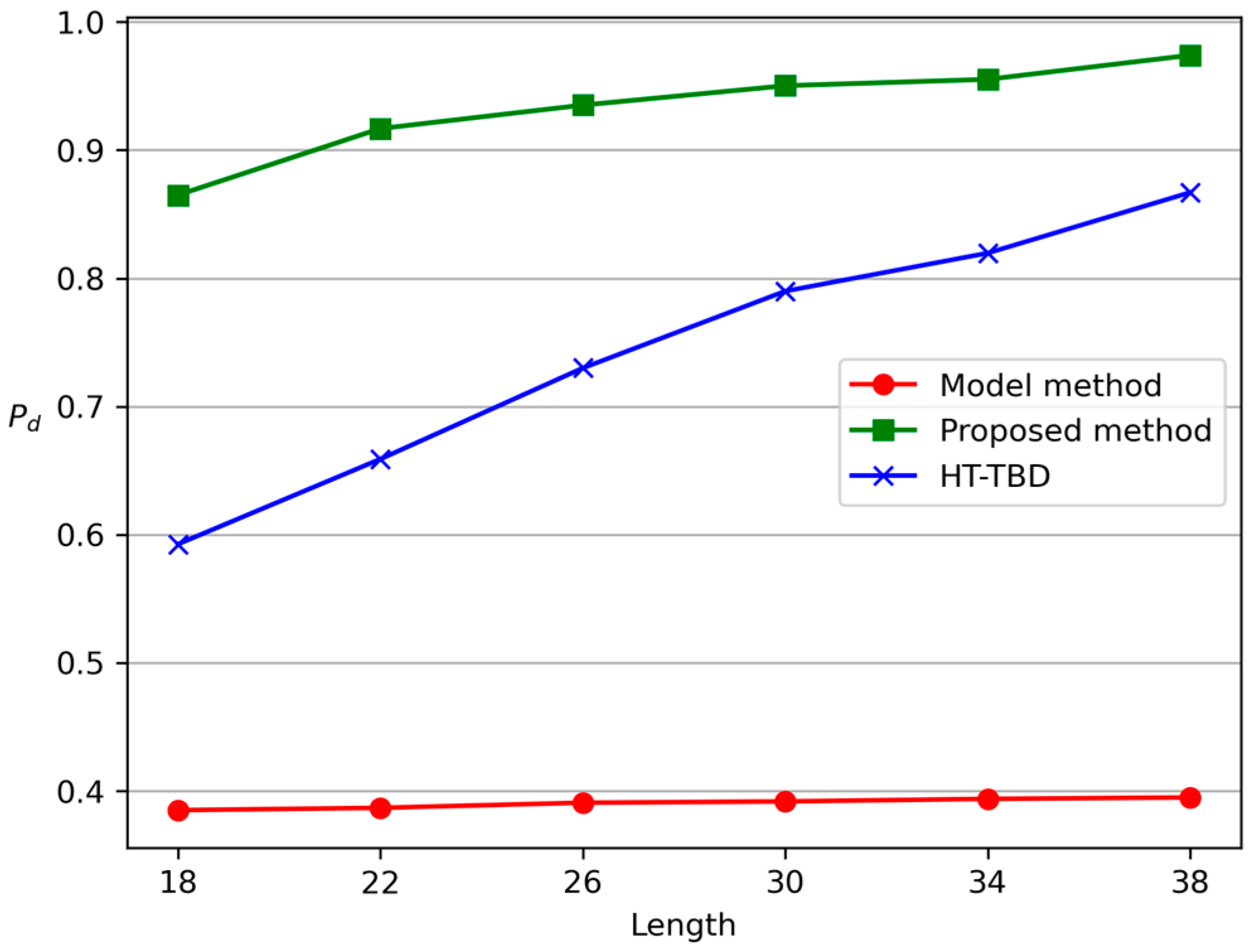
3.4. Detection Performance Analysis

In order to conduct a more quantitative evaluation of the method presented in this paper, the false alarm probability and detection probability with different processing frames were analyzed. Since a single scene is not universal, we conducted experiments on 200 scenes to obtain the change curve of the number of processing frames with the false track rate and detection probability. The corresponding curves were compared with the results obtained via only the model method and the HT-TBD method.

The false alarm probability is the probability that a false target is judged as a target [41]. When calculating the false alarm rate of the model’s decision results in this study, it is necessary to carry out a transformation, as in Equation (20). Here, $P_{fa}$ represents the false alarm rate; $Q$ represents the number of Monte Carlo simulations; $N_{fa}(i)$ represents the number of false tracks judged by the model after the $i$-th Monte Carlo simulation; and $N_{tot}(i)$ represents the number of all detection units in the $i$-th Monte Carlo simulation. The curves of the false alarm rate with the number of processed frames are shown in Figure 11.

$$P_{fa}=\frac{{\displaystyle \sum _i^Q{N}_{fa}(i)}}{{\displaystyle \sum _i^Q{N}_{tot}(i)}}$$

(20)

It can be observed from Figure 11 that the false alarm rate obtained only by the model method was higher, and its change with the number of processing frames was not significant. Compared with the model method, the false alarm rate of HT-TBD was lower and reached below 10⁻² with the increase in the number of processing frames. Compared with the previous two methods, the proposed method had a lower overall false alarm rate. At the same time, the false alarm rate decreased significantly with the increase in the number of processing frames. When the number of processing frames was more than 26, the false alarm rate decreased to 10⁻³.

The detection probability can be expressed as the quotient obtained by dividing the total number of times a target is correctly detected by the overall number of target occurrences, as shown in Equation (21). In this equation, $N_d(i)$ is the number of targets obtained after processing in the $i$-th Monte Carlo simulation. The curves of detection probability with the number of processing frames are shown in Figure 12.

$$P_d=\frac{{\displaystyle \sum _i^Q{N}_d(i)}}{{\displaystyle \sum _i^Q{N}_{tot}(i)}}$$

(21)

From Figure 12, it is evident that the detection probability achieved solely by the model method was low and showed minimal variation with the number of processed frames. The detection probability of HT-TBD increased with the increase in the number of processing frames. This can be attributed to the fact that as the number of processing frames increased, the accumulation of histogram energy in the parameter space became stronger. In comparison with the previous two methods, the proposed method exhibited an increasing detection probability with an increase in the number of processing frames. Specifically, when the number of processing frames reached 38, the detection probability reached 0.97. To better illustrate the performance of the proposed method, we conducted simulation experiments on typical scenarios with 25 false alarms per frame. Figure 13a–c illustrates a typical scene with seven moving targets. From Figure 13a, it can be observed that the clutter was dense, and it was difficult to distinguish several of the moving targets. Figure 13b shows the results of using the model method. It can be observed that the majority of the clutter can be eliminated through processing; however, the resulting track appears disorganized and contains numerous false tracks. Figure 13c shows the result of HT-TBD processing. It is evident that HT-TBD exhibited superior tracking performance for linearly moving targets; however, its effectiveness diminished when tracking targets with specific maneuvers, while also accentuating false tracks in clutter-dense areas. Figure 14a,b show the results of track-before-detect based on multi-frame structural information. It can be noted that when the number of processing frames was set to 18, a significant reduction in false tracks in Figure 14b can be witnessed, although some remnants still persist. With the progressive increase in the number of processing frames, the false tracks gradually diminished, eventually resulting in the retention of the final seven authentic targets.

To validate comprehensively the effectiveness of the method proposed in this paper, experiments were conducted in the same typical scenario, but with the number of false alarms per frame set to 40. The results in Figure 15a–c and Figure 16a,b show that as the number of false alarms increased, the model method clearly produced more false tracks, and the track obtained by the HT-TBD method was also poor. In comparison, although the proposed method still had a small quantity of false tracks when processing 18 frames and 38 frames, it could better eliminate false tracks and retain the true ones, compared with the previous two methods.

4. Discussion

Non-cooperative bistatic radar systems are affected by decreases in the space and time synchronization accuracies. The target position accuracy and echo SNR ratio are low, and the detection between target frames is unstable. It is difficult to achieve effective tracking of the target if the traditional DBT method is used. Therefore, scholars have proposed a TBD method to solve the target tracking problem in non-cooperative bistatic radar scenarios. However, most of the existing research in this area is based on civil signals, with few studies involving radar signals as non-cooperative radiation sources. Furthermore, there are relatively few references on combining TBD with deep learning. Most studies apply deep learning methods to data preprocessing, such as using neural networks to highlight potential motion patterns of targets or enhance the extraction capability of weak targets. Essentially, this approach extracts potential features before traditional TBD processing, rather than integrating the feature extraction process into the TBD processing framework.

In view of the above problems, this work draws on the idea of the two-stage TBD and uses the powerful fitting ability of neural networks to learn the complex mapping relationship between multi-dimensional features and serialized target track decision to propose a two-stage track-before-detect method for non-cooperative bistatic radar based on deep learning. On the one hand, the proposed method exhibits superior generalization ability and tracking accuracy compared with HT-TBD, which also uses a batch processing approach. On the other hand, the proposed method employs a low threshold to minimize data processing and ensure a certain level of real-time performance. In addition, reference [42] proposed a TBD method based on parallel-line–coordinate transformation, which is also aimed at solving the problem of high computational complexity in HT-TBD. When applied to simulation data with a single frame of approximately 20 false alarms, the method required 1.0146 s to run, while in our experiments with a single frame of approximately 25 false alarms, it only required 0.353684 s to run. It can be observed that the method described in this paper significantly diminishes the computational load.

The effectiveness of the method proposed in this paper stems from its departure from the traditional TBD method, which invariably incorporates an explicit or implicit modeling of the target motion. Consequently, when the track of the target cannot be accurately captured by a specific mathematical model, the tracking performance suffers. Moreover, with an increase in the number and complexity of targets, the computational demands of the TBD method escalate, leading to a decrease in the processing speed. It is worth highlighting that the data collected in this study originated exclusively from stationary platforms. Nevertheless, non-cooperative bistatic radar can also be extended to mobile platforms, such as unstaffed boats, due to its cost-effectiveness and compact size. Our team has already commenced experimentation on a mobile offshore platform; however, it is imperative to conduct thorough analyses and verification of any potential issues that may emerge during these experiments. Furthermore, in the two-stage track-before-detect method based on deep learning, we have the opportunity to integrate additional features to enhance the effectiveness of the tracking. Further deliberation is required to identify the specific features that warrant more extensive investigation.

5. Conclusions

This paper presents a two-stage track-before-detect method for non-cooperative bistatic radar, employing deep learning techniques. Firstly, a low-threshold target detection network is utilized to ensure that the target is detected within the desired threshold. Next, the model method is employed to identify potential tracks. Subsequently, position information, innovation score, and structural information of the target are extracted using convolutional networks, fully connected networks, and LSTM networks. The predicted tracks are obtained, resulting in the tracking outcome for the target. Additionally, this paper utilizes radar signals as non-cooperative radiation sources for experimental validation. The experimental results demonstrate that this method effectively eliminates false tracks, and the tracking performance improves with the increase in the number of frames processed. Thus, the proposed two-stage track-before-detect method for non-cooperative bistatic radar, based on deep learning, offers an effective solution for target tracking in non-cooperative bistatic radar systems.

References

1. Bao, Q.L.; Sen, W.; Pan, J.M.; Zhu, X. Analysis of key technologies of non-cooperative radar emitter target detection system. J. Radio Wave Sci. 2020, 35, 496–503. [Google Scholar] [CrossRef]
2. Mao, E.K.; Zeng, T.; Hu, C.; Long, T. Bistatic detection system based on geosynchronous synthetic aperture radar: Concept and potential. Signal Process. 2013, 29, 285–292. [Google Scholar]
3. Ge, X.J.; He, Y.; Song, J. Complex envelope estimation technology of direct wave pulse based on improved CMA + MMA. Mod. Radar 2010, 32, 54–59. [Google Scholar] [CrossRef]
4. Xi, Z. Research on Key Technologies of Clutter Interference Suppression and Target Tracking for Non-Cooperative Bistatic Radar. Ph.D. Thesis, National University of Defense Technology, Changsha, China, 2020. [Google Scholar]
5. Yi, W. Research on multi-target tracking algorithm based on track-before-detect technology. Ph.D. Thesis, University of Electronic Science and Technology of China, Chengdu, China, 2012. [Google Scholar]
6. Fu, L.Z.; Wang, B.; Cao, Y.; Yi, W. Multi-station anti-radiation radar target tracking algorithm based on PF-TBD. In Proceedings of the Tenth China Aviation Association Youth Science and Technology Forum Papers, Nanchang, China, 19–20 November 2022; pp. 406–411. [Google Scholar]
7. Lehmann, F. Recursive Bayesian filtering for multitarget track-before-detect in passive radars. IEEE Trans. Aerosp. Electron. Syst. 2012, 48, 2458–2480. [Google Scholar] [CrossRef]
8. Santi, F.; Pastina, D.; Bucciarelli, M. Experimental demonstration of ship target detection in GNSS-based passive radar combining target motion compensation and track-before-detect strategies. Sensors 2020, 20, 599. [Google Scholar] [CrossRef] [Green Version]
9. Knoedler, B.; Steffes, C.; Koch, W. Detecting and tracking a small UAV in GSM passive radar using track-before-detect. In Proceedings of the 2020 IEEE Radar Conference (RadarConf20), Florence, Italy, 21–25 September 2020; pp. 1–6. [Google Scholar]
10. Li, Y.; Ma, H.; Wu, Y.; Cheng, L. Track-Before-Detect Procedures in AM Radio-Based Passive Radar. Int. J. Antennas Propag. 2021, 2021, 3911956. [Google Scholar] [CrossRef]
11. Testolin, A.; Diamant, R. Combining denoising autoencoders and dynamic programming for acoustic detection and tracking of underwater moving targets. Sensors 2020, 20, 2945. [Google Scholar] [CrossRef]
12. Carr, C.; Dang, B.; Metcalf, J. RADGAN: Applying adversarial machine learning to track-before-detect radar. In Proceedings of the 2021 IEEE Radar Conference (RadarConf21), Atlanta, GA, USA, 7–14 May 2021; pp. 1–6. [Google Scholar]
13. Wen, L.; Zhong, C.; Huang, X.; Ding, J. Sea clutter suppression based on selective reconstruction of features. In Proceedings of the 2019 6th Asia-Pacific Conference on Synthetic Aperture Radar (APSAR), Xiamen, China, 26–29 November 2019; pp. 1–6. [Google Scholar]
14. Wen, L.; Ding, J.; Xu, Z. Multiframe detection of sea-surface small target using deep convolutional neural network. IEEE Trans. Geosci. Remote Sens. 2021, 60, 5107116. [Google Scholar] [CrossRef]
15. Zhu, C.; Deng, J.; Long, X.; Zhang, W.; Yi, W. DBU-Net Based Robust Target Detection for Multi-Frame Track-Before-Detect Method. In Proceedings of the 2022 11th International Conference on Control, Automation and Information Sciences (ICCAIS), Hanoi, Vietnam, 21–24 November 2022; pp. 412–418. [Google Scholar]
16. Grossi, E.; Lops, M.; Venturino, L. A novel dynamic programming algorithm for track-before-detect in radar systems. IEEE Trans. Signal Process. 2013, 61, 2608–2619. [Google Scholar] [CrossRef]
17. Song, J.; Xiong, W.; Chen, X.; Lu, Y. Experimental study of maritime moving target detection using hitchhiking bistatic radar. Remote Sens. 2022, 14, 3611. [Google Scholar] [CrossRef]
18. Pan, M.; Chen, J.; Wang, S.; Dong, Z. A novel approach for marine small target detection based on deep learning. In Proceedings of the 2019 IEEE 4th International Conference on Signal and Image Processing (ICSIP), Wuxi, China, 19–21 July 2019; pp. 395–399. [Google Scholar]
19. Shao, Y.E. Multi-Static Passive Radar Target Location and Tracking Based on Navigation Satellite. Master’s Thesis, Xi’an University of Electronic Science and Technology, Xi’an, China, 2022. [Google Scholar]
20. Chen, X. Research on Improved Radar Multi-Target Track Initiation Algorithm. Master’s Thesis, Dalian Maritime University, Dalian, China, 2021. [Google Scholar]
21. Mayor, M.A.; Carroll, R.L. A multi-target track initiation algorithm. In Proceedings of the 1987 American Control Conference, Minneapolis, MN, USA, 10–12 June 1987; pp. 1128–1130. [Google Scholar]
22. Trunk, G.; Wilson, J. Track initiation of occasionally unresolved radar targets. IEEE Trans. Aerosp. Electron. Syst. 1981, AES-17, 122–130. [Google Scholar] [CrossRef]
23. Zhao, C.C.; Wang, J.; Shao, L. Basic algorithm for trajectory initiation of ballistic target based on grid clustering. Fire Control. Command. Control. 2018, 43, 37–41+46. [Google Scholar]
24. Smith, M. Feature space transform for multitarget detection. In Proceedings of the 1980 19th IEEE Conference on Decision and Control including the Symposium on Adaptive Processes, Albuquerque, NM, USA, 10–12 December 1980; pp. 835–836. [Google Scholar]
25. Li, J.Q.; Zhao, R.H.; Xu, J.L.; Zhao, C.Y.; Ge, J.X. Trajectory initiation based on ant colony similarity weighted Hough transform. J. Sens. Technol. 2016, 29, 552–558. [Google Scholar]
26. Shen, G.M.; Xiong, X.; Fan, Y.Q. Trajectory Initiation Method Based on Spatio-Temporal Characteristics of Radar Measurements. J. Terahertz Sci. Electron. Inf. 2022, 20, 1269–1276. [Google Scholar]
27. He, Y.; Xiu, J.J.; Zhang, J.W. Radar Data Processing and Application, 2nd ed.; Electronic Industry Press: Beijing, China, 2009; pp. 91–93. [Google Scholar]
28. Tan, S.C.; Wang, G.H.; Wang, N. IMM-Singer Model Based Tracking Algorithm for Maneuvering Targets. Fire Control. Command. Control. 2012, 37, 32–34. [Google Scholar]
29. Singer, R.A. Estimating optimal tracking filter performance for manned maneuvering targets. IEEE Trans. Aerosp. Electron. Syst. 1970, AES-6, 473–483. [Google Scholar] [CrossRef]
30. Wang, J.; Yi, W.; Kong, L. Improved DP-TBD methods based on multiple hypothesis testing for target early detection. In Proceedings of the 2016 19th International Conference on Information Fusion (FUSION), Heidelberg, Germany, 5–8 July 2016; pp. 1406–1413. [Google Scholar]
31. Raghu, M.; Poole, B.; Kleinberg, J.; Ganguli, S.; Sohl-Dickstein, J. On the expressive power of deep neural networks. In Proceedings of the International Conference on Machine Learning, Sydney, NSW, Australia, 6–11 August 2017; pp. 2847–2854. [Google Scholar]
32. Fan, W.T.; Li, Z.Y.; Zhang, T.; Luo, X.Y. Analysis of JPEG steganography based on deep extraction of steganographic noise. J. Xidian Univ. 2022, 50, 1–13. [Google Scholar]
33. Hornik, K. Approximation capabilities of multilayer feedforward networks. Neural Netw. 1991, 4, 251–257. [Google Scholar] [CrossRef]
34. Riedmiller, M. Advanced supervised learning in multi-layer perceptrons—From backpropagation to adaptive learning algorithms. Comput. Stand. Interfaces 1994, 16, 265–278. [Google Scholar] [CrossRef]
35. Zhang, W.; Tanida, J.; Itoh, K.; Ichioka, Y. Shift-invariant pattern recognition neural network and its optical architecture. In Proceedings of the Annual Conference of the Japan Society of Applied Physics, Canada, 1988; pp. 2147–2151. [Google Scholar]
36. Mikolov, T.; Kombrink, S.; Burget, L.; Černocký, J.; Khudanpur, S. Extensions of recurrent neural network language model. In Proceedings of the 2011 IEEE International Conference on Acoustics, Speech and Signal Processing (ICASSP), Prague, Czech Republic, 22–27 May 2011; pp. 5528–5531. [Google Scholar]
37. Luo, Z. Research on track-before-detect and fusion technology of weak target. Ph.D. Thesis, Xi’an University of Electronic Science and Technology, Xi’an, China, 2019. [Google Scholar]
38. Wang, J.H.; Yi, W.; Kong, L.J. Research on multi-frame track- before-detect algorithm for netted radar. J. Radars 2019, 8, 490–500. [Google Scholar]
39. Terrell, G.R.; Scott, D.W. Variable kernel density estimation. Ann. Stat. 1992, 20, 1236–1265. [Google Scholar] [CrossRef]
40. Carlson, B.; Evans, E.; Wilson, S. Search radar detection and track with the Hough transform. I. system concept. IEEE Trans. Aerosp. Electron. Syst. 1994, 30, 102–108. [Google Scholar] [CrossRef]
41. Ding, L.F. Radar Principles, 3rd ed.; National Defense Industry Press: Beijing, China, 2009. [Google Scholar]
42. Bo, J.T.; Wang, G.H.; Yu, H.B.; Peng, Z.G. Track-before-detect algorithm based on parallel-line-coordinate transformation. Acta Aeronaut. Astronaut. Sin. 2022, 43, 570–583. [Google Scholar]
Figure 1. Working principle of the non-cooperative bistatic radar system.
Remotesensing 15 03757 g001
Figure 2. Signal processing flow chart of the non-cooperative bistatic radar system.
Remotesensing 15 03757 g002
Figure 3. PPI of adjacent frames: (a) Previous frame; (b) Next frame.
Remotesensing 15 03757 g003
Figure 4. Integral structure.
Remotesensing 15 03757 g004
Figure 5. Network structure.
Remotesensing 15 03757 g005
Figure 6. LSTM network structure.
Remotesensing 15 03757 g006
Figure 7. Experimental area.
Remotesensing 15 03757 g007
Figure 8. Accuracy curve of different track lengths.
Remotesensing 15 03757 g008
Figure 9. PDFs of the confidence scores for different numbers of processed frames for true tracks (the label ‘PDF’ represents the kernel density estimation method, and the label ‘Data’ represents the original confidence histogram distribution of the true track). (a) 18 frames; (b) 22 frames; (c) 26 frames; (d) 30 frames; (e) 34 frames; (f) 38 frames.
Remotesensing 15 03757 g009
Figure 10. PDFs of the confidence scores for different numbers of processed frames for false tracks (the label ‘PDF’ represents the kernel density estimation method, and the label ‘Data’ represents the original confidence histogram distribution of the false track). (a) 18 frames; (b) 22 frames; (c) 26 frames; (d) 30 frames; (e) 34 frames; (f) 38 frames.
Remotesensing 15 03757 g010aRemotesensing 15 03757 g010b
Figure 11. Relationship between false alarm rate and the number of frames processed.
Remotesensing 15 03757 g011
Figure 12. Relationship between detection probability and track length.
Remotesensing 15 03757 g012
Figure 13. Typical scene with 25 false alarms per frame: (a) 40 frame low-threshold detection results (different colors represent the detection results of different frames); (b) tracks formed by the model method; (c) tracks formed by HT-TBD.
Remotesensing 15 03757 g013
Figure 14. Results of the two-stage track-before-detect model based on deep learning (25 false alarms per frame): (a) 18 processed frames; (b) 38 processed frames.
Remotesensing 15 03757 g014
Figure 15. Typical scene with 40 false alarms per frame: (a) 40 frames low-threshold detection results (different colors represent the detection results of different frames); (b) tracks formed by the model method; (c) tracks formed by HT-TBD.
Remotesensing 15 03757 g015
Figure 16. Results of the two-stage track-before-detect model based on deep learning (40 false alarms per frame): (a) 18 processed frames; (b) 38 processed frames.
Remotesensing 15 03757 g016