Micromotion Feature Extraction with VEMW Radar Based on Rotational Doppler Effect

Abstract

Micro-Doppler (m-D) analysis is the most effective mechanism for detecting rotating targets or components; however, it fails when the target rotation plane is perpendicular to the radar line of sight (LOS). The vortex electromagnetic wave (VEMW) provides a unconventional structure of wavefront phase modulation on the cross-plane of the radar LOS, on which the radial m-D vanishes while the rotational Doppler (RD) appears. In the absence of the position of rotation center, this paper focuses on the micromotion parameters estimation based on RD effect for rotating target, and then proposes an estimation procedure, referred to as the two-step method. The micromotion parameters of the rotating target include the rotation attitude, the rotation radius and the position of the rotation center while the latter is coupled to the former two. Firstly, the micromotion parameters are roughly estimated based on the RD curve parameters obtained from the time-frequency (TF) spectrum of the received signal. Secondly, the maximum likelihood estimation (MLE) is used to accurately estimate the micromotion parameters. In addition, the Cramér–Rao bound (CRB) of parameter estimation is derived. The simulation studies the influencing factors of estimation performance and verifies that the proposed estimation method can provide excellent estimation accuracy of the micromotion parameters.

1. Introduction

The Doppler effect represents the radial velocity between target and radar. However, when the velocity of the target is perpendicular to the radar line of sight (LOS), the faint Doppler component is difficult to extract from the received signals, which makes the detection of target motion blind. In 1992, orbital angular momentum (OAM) in Laguerre–Gauss (LG) vortex beam was discovered as another intrinsic of electromagnetic wave following amplitude, phase, frequency, and polarization [1]. When the electromagnetic wave with OAM vertically irradiates the target rotation plane, an effect similar to the radial Doppler frequency shift occurs, which is called the rotational Doppler (RD) effect. Therefore, the vortex electromagnetic wave (VEMW) radar cannot only detect the radial motion of the target, but also obtain the angular motion information (angular frequency, angular acceleration, etc.) of the target.

The research of the RD effect began with optics. Benefited from their collimation, vortex beams are easy to fabricate large topological charges. A LG vortex beam with mode l formed a frequency difference of $2l\omega$ after passing through a prism with an angular frequency $\omega$ [2]. The concept of the RD shift was later introduced in [3]. Afterwards, Courtial observed the frequency shift, $l\omega$, imparted to a mm-wave beam with an OAM of $l\hslash$ per photon, when the beam is rotating with an angular frequency $\omega$ [4]. The above studies found the corresponding relationship among vortex beams and rotating objects, but did not give the quantitative relationship among them which was obtained with the optical experiments [5]. In addition, the formulation of RD frequency was derived according to the radial Doppler frequency, and the consistency of the two was proved.

No beat frequency signal is required for microwave band compared with the optical band, so that the received signal with Doppler frequency was processed more easily. Unlike the radial Doppler, which only depends on the radial velocity, the RD effect is determined by the change of the target azimuth, that is, the angular frequency and the position of the target in the vortex field [6,7]. The RD effect is obvious to detect when the angular frequency and the VEMW beam axis are collinear. In 2016, the RD effect in the microwave band was experimentally verified by the phase accumulation method [8]. Afterwards, the RD effect of uniformly accelerated rotating target was studied based on the time-frequency (TF) analysis methods, including Wigner–Ville distribution (WVD) and fractional fourier transform (FRFT) [9]. The target instantaneous angular frequency was estimated by means of the spectrum analysis, and the rotation direction was obtained according to the position of the side lobes [10]. The RD effect is quite complex when the angular velocity and the VEMW beam axis are not collinear. In 2018, the effects of the rotation plane deflection and non-coaxial placement of the transceiver antenna on the RD shift were investigated, simultaneously, the scattered wave was derived and verified experimentally at 10 GHz [11]. In 2020, the RD effect was derived when the normal of the rotation plane deviates from the VEMW beam axis. On this basis, a parameter estimation method was proposed, including the rotation radius and the angular frequency of the rotating target [12]. The RD effect of rotating target at arbitrary positions was studied in [13]. In 2021, the Doppler component decoupling method and the micromotion feature extraction algorithm of the rotating target composed of multiple scattering points were proposed, and the deflection angle of the rotation plane was estimated [14,15]. In 2022, based on the RD effect, the micro Doppler parameter extraction of precession cone-shaped targets and spinning targets were studied [16,17]. The study of the RD effect is limited by its small amplitude, which depends on the OAM mode number and angular frequency. In addition, the energy divergence of VEMW leads to low energy utilization. From the perspective of the research object, the research of RD effect has experienced three stages comprised of the phase and spectrum analysis of the disk, the modeling and experimental verification of the point target, and the theoretical analysis of the complex target.

The previous micromotion parameters estimation researches of the VEMW radar were based on the assumption that the position of rotation center is accurately known which is impractical. The limited radar resolution, which depends on the signal bandwidth and array aperture, makes the position of the rotation center inaccurate. Under limited radar resolution, the estimation deviation of the rotation center position can render the existing observation model or estimation algorithm ineffective. Therefore, this paper aims to extract the micromotion parameters of the RD effect and derive the Cramér–Rao bound (CRB) of parameter estimation when the position of the rotation center is unavailable. Without loss of rationality, it is assumed that the rotating target has been detected with a fairly coarse set of range cells. Firstly, on the basis of [13,14], we derive the analytical solution of the micromotion parameters of rotating target based on the smooth pseudo Wigner–Ville distribution (SPWVD) spectrum which has high TF resolution. Secondly, the maximum likelihood estimation (MLE) of micromotion parameters is obtained with the particle swarm optimization (PSO) algorithm based on the previous rough estimation. Subsequently, the CRB is derived. Due to the bias of SPWVD spectrum, the mean square error (MSE) of rough estimation based on SPWVD spectrum deviates greatly from the CRB. The MSE of MLE is close to CRB in the dynamic range of signal-to-noise ratio (SNR). Finally, the numerical experiments are conducted to verify the effectiveness of the micromotion parameters estimation method and analyze the influence of angular frequency and the micromotion parameters on the final estimated performance.

The rest of this paper is organized as follows. Section 2 formulates the signal model and the analysis of RD effect based on the VEMW radar system. Section 3 presents a two-step micromotion parameters estimation approach and derives the CRB of the parameters estimation. Section 4 presents extensive simulation results. Finally, Section 5 provides summaries and concluding remarks.

2. Signal Model

The micromotion parameters estimation of radar target has attracted extensive research attention over the past decade. As a common micromotion, rotation is the basic motion component of radar target or its component. The RD effect caused by rotation based on the VEMW radar is studied in this section.

2.1. Observation Model

Up to the present, there are numerous ways to generate VEMW. For radar applications, it can be generated in a simple way by an incrementally phased uniform circular array (UCA) [18], as shown in Figure 1. $OXYZ$ is a radar Cartesian coordinate system centered on the origin O. N antennas are equidistantly arranged along the circumference on the $XOY$ plane with radius a. The transmitted signals are phased with $e^{jl{\varphi }_n}$, where ${\varphi }_n=2n/N,n=1,2,\cdots ,N$, l denotes the OAM mode number. The origin o of the reference coordinate system $o{X}^{\prime }{Y}^{\prime }{Z}^{\prime }$, which is parallel to the radar coordinate system, is located at $(X_o,Y_o,Z_o)$ in the radar coordinate system. The target-local coordinate system $oxyz$ shares the same origin o. The scattering point q rotates around the z-axis on the $xoy$ plane with the origin o as the rotation center. The angular frequency is $\omega$, and the rotation radius is $r_a$. Therefore, the Cartesian coordinates of the scattering point q at time t in the target-local coordinate system is

$${\left[x_q\left(t\right),y_q\left(t\right),z_q\left(t\right)\right]}^{\mathrm{T}}={\left[r_{a}cos\left(\omega t\right),r_{a}sin\left(\omega t\right),0\right]}^{\mathrm{T}}.$$

(1)

In order to transform the coordinates of the scattering point q into the radar coordinate system, it is necessary to introduce the Euler angle. As shown in Figure 1b, the Euler angle between the reference coordinate system $o{X}^{\prime }{Y}^{\prime }{Z}^{\prime }$ and the target-local coordinate system $oxyz$ is $\left(\alpha ,\beta ,\gamma \right)$, i.e., the reference coordinate system can be transformed to the target-local coordinate system by rotating about the $Z^{\prime }$-axis for $\alpha$, the $X^{\prime }$-axis for $\beta$ and the $Z^{\prime }$-axis again for $\gamma$. $\alpha$ and $\beta$ correspond to the rotational attitude, while $\gamma$ represents the initial phase of rotation. Then the Cartesian coordinates of scattering point q at time t in the radar coordinate system can be expressed as [19]

$$\begin{array}{c}\left[\begin{array}{c}{X}_q\left(t\right)\\ Y_q\left(t\right)\\ Z_q\left(t\right)\end{array}\right]=\mathbf{R}\left(\alpha ,\beta ,\gamma \right)·\left[\begin{array}{c}{x}_q\left(t\right)\\ y_q\left(t\right)\\ z_q\left(t\right)\end{array}\right]+\left[\begin{array}{c}{X}_o\\ Y_o\\ Z_o\end{array}\right],\end{array}$$

(2)

where $R\left(\alpha ,\beta ,\gamma \right)$ is the Euler matrix. It can be represented in the spherical coordinate system $\left(r,\theta ,\phi \right)$ by

$$r_q\left(t\right)=\sqrt{X_q{\left(t\right)}^2+Y_q{\left(t\right)}^2+Z_q{\left(t\right)}^2},$$

(3)

$${\theta }_q\left(t\right)=\mathrm{asin}(\sqrt{X_q{\left(t\right)}^2+Y_q{\left(t\right)}^2}/r_q\left(t\right)),$$

(4)

$${\phi }_q\left(t\right)=\mathrm{atan}(Y_q\left(t\right)/X_q\left(t\right)),$$

(5)

where $r_q\left(t\right),{\theta }_q\left(t\right),{\phi }_q\left(t\right)$ denote the radial distance, polar angle and azimuthal angle, respectively, and ${\theta }_q\left(t\right)\in [0,\pi )$, ${\phi }_q\left(t\right)\in [0,2\pi )$. When the projection length of $r_a$ on the $X^{\prime }o{Y}^{\prime }$ plane is much less than $r_q\left(t\right)$, (3) can be rewritten approximately as [19]

$$r_q\left(t\right)\approx r_{a\mathrm{LOS}}sin\left(\omega t\right)+r_0,$$

(6)

where $r_{a\mathrm{LOS}}$ is the maximum projection length of $r_a$ on the LOS during the rotation of q, $r_0=\sqrt{X_o^2+Y_o^2+Z_o^2}$ is the distance from o to O.

Furthermore, we have

$$\begin{array}{cc}\hfill {\phi }_q\left(t\right)& =\mathrm{atan}\left(\frac{-sin({\phi }_o-\alpha )cos(\omega t+\gamma )+cos({\phi }_o-\alpha )cos\beta sin(\omega t+\gamma )}{cos({\phi }_o-\alpha )cos(\omega t+\gamma )+sin({\phi }_o-\alpha )cos\beta sin(\omega t+\gamma )+{\rho }_o/r_a}\right)+{\phi }_o,\hfill \end{array}$$

(7)

where ${\rho }_o=\sqrt{X_o^2+Y_o^2}$ is the deflection distance from the rotation center o to VEMW beam axis, i.e., Z-axis; ${\phi }_o=\mathrm{atan}\left(Y_o/X_o\right)$ represents the azimuth angle of rotation center o in $OXYZ$. In this paper, the deflection distance ${\rho }_o$ and the azimuth angle of rotation center ${\phi }_o$ are assumed unavailable. For simplification, ${\phi }_{\alpha }$ is used to replace $({\phi }_o-\alpha )$ and ${\varphi }_t$ replaces $(\omega t+\gamma )$.

2.2. Vortex Signal Model

The linear frequency modulation (LFM) signal is selected as the transmitting signal for each element of the UCA, which can be given as

$$s_{\mathrm{trans}}\left(\tau \right)=\mathrm{rect}\left(\frac{\tau }{T}\right)e^{j2\pi \left(f_0\tau +0.5K{\tau }^2\right)},$$

(8)

where $\mathrm{rect}\left(\tau /T\right)$ is a rectangular window, T is the pulse duration, $f_0$ is the carrier frequency, K is the frequency modulation rate. The received signal of the scattering point q is

$$\begin{array}{c}\hfill s(\tau ,t,l)=j^l{\sigma }_{q}N{J}_l\left[k\left(\tau -{\tau }_q\left(t\right)\right)asin{\theta }_q\left(t\right)\right]e^{jl{\phi }_q\left(t\right)}·\mathrm{rect}\left(\frac{\tau -{\tau }_q\left(t\right)}{T}\right)e^{j2\pi \left(f_0\left(\tau -{\tau }_q\left(t\right)\right)+0.5K{\left(\tau -{\tau }_q\left(t\right)\right)}^2\right)},\end{array}$$

(9)

where ${\sigma }_p$ is the scattering coefficient of the scattering point q; N represents the number of UCA antennas used to generate VEMW; k is the wavenumber which is the function of fast time $\tau$; ${\tau }_q\left(t\right)=2r_q\left(t\right)/c$; c is the speed of light; $J_l(·)$ is the first kind of l-order Bessel function. It is assumed that the reference signal is $s_{\mathrm{ref}}\left(\tau \right)=\mathrm{rect}(\tau /T)e^{-2\pi (f_0\tau +0.5K{\tau }^2)}$. Multiplying $s(\tau ,t,l)$ by the reference signal $s_{\mathrm{ref}}\left(\tau \right)$ yields [14]:

$$s_1(\tau ,t,l)=j^l{\sigma }_{q}N{J}_l\left[k\left(\tau -{\tau }_q\left(t\right)\right)asin{\theta }_q\left(t\right)\right]e^{jl{\phi }_q\left(t\right)}·\mathrm{rect}\left(\frac{\tau -{\tau }_q\left(t\right)}{T}\right)e^{j2\pi \left(0.5K{\tau }_q^2\left(t\right)-f_0{\tau }_q\left(t\right)-K{\tau }_q\left(t\right)\tau \right)}.$$

(10)

After performing the fast Fourier transform (FFT) in the fast time $\tau$ dimension, $s_1(\tau ,t,l)$ is transformed into

$$S(f_{\tau },t,l)=j^l{\sigma }_{q}NH\left(f_{\tau }+K{\tau }_q\left(t\right)\right)e^{jl{\phi }_q\left(t\right)}·e^{-j\pi \left(f_{\tau }+K{\tau }_q\left(t\right)\right){\tau }_q\left(t\right)}{e}^{j2\pi \left(0.5K{\tau }_q^2\left(t\right)-f_0{\tau }_q\left(t\right)\right)},$$

(11)

where $H\left[f_{\tau }+K{\tau }_q\left(t\right)\right]=\mathrm{FFT}\left[J_l\left(k\left(\tau \right)\right)\mathrm{rect}(\tau /T)\right]$, whose properties are similar to the sinc function [14]. Assuming that the rotating target q is located in the range resolution cell $f_{\tau }=-K{\tau }_q\left(t\right)$. Substituting $f_{\tau }=-K{\tau }_q\left(t\right)$ into (9) yields

$$S_2(f_{\tau },t,l)=j^l{\sigma }_{q}NH\left(0\right)e^{jl{\phi }_q\left(t\right)}{e}^{-j2\pi f_0{\tau }_q\left(t\right)}·e^{j\pi f_{\tau }^2/K},$$

(12)

where $e^{j\pi f_{\tau }^2/K}$ is the residual video phase (RVP) term. Using $e^{-j\pi f_{\tau }^2/K}$ to compensate for the RVP term, the peak signal $s_{\mathrm{peak}}(t,l)$ of (11) can be expressed as

$$\begin{array}{c}{s}_{\mathrm{peak}}(t,l)=j^l{\sigma }_{q}NH\left(0\right)e^{jl{\phi }_q\left(t\right)}{e}^{-j2\pi f_0{\tau }_q\left(t\right)}.\end{array}$$

(13)

2.3. Doppler Effect

The phase term of the processed signal $s_{\mathrm{peak}}(t,l)$ can be expressed as $\Phi \left(t\right)=-2\pi f_0{\tau }_q\left(t\right)+l{\phi }_q\left(t\right)$. As shown in Figure 2, the coloured vortex curves depict the phase front distribution of the electric field in a plane parallel to the $XOY$ plane. The change of color from blue to yellow corresponds to the change of phase from $-\pi$ rad to $\pi$ rad. It can be observed that the movement of the scattering point q in the LOS direction produces a linear Doppler effect, which changes the phase term $e^{-2\pi f_0{\tau }_q\left(t\right)}$. The motion perpendicular to the LOS produces a RD effect, resulting in a change in the phase term $e^{jl{\phi }_q\left(t\right)}$. The theoretical Doppler shift of the processed signal can be derived as

$$f_D\left(t\right)=\frac{1}{2\pi }\frac{\mathrm{d}\Phi \left(t\right)}{\mathrm{d}t}=-f_0\frac{\mathrm{d}{\tau }_q\left(t\right)}{\mathrm{d}t}+\frac{l}{2\pi }\frac{\mathrm{d}{\phi }_q\left(t\right)}{\mathrm{d}t}=f_L+f_R.$$

(14)

Therefore, the linear m-D frequency shift $f_L\left(t\right)$ of the scattering point q is

$$f_L\left(t\right)=-f_0\frac{\mathrm{d}{\tau }_q\left(t\right)}{\mathrm{d}t}=\frac{2f_0\omega r_{a\mathrm{LOS}}}{c}cos\left(\omega t\right),$$

(15)

which is consistent with the m-D effect of rotation in plane electromagnetic wave radar. The RD frequency shift $f_R\left(t\right)$ of the scattering point q can be written as

$$\begin{array}{cc}\hfill f_R\left(t,\mathbf{\eta }\right)& =\frac{l}{2\pi }\frac{\mathrm{d}{\phi }_q\left(t\right)}{\mathrm{d}t}\hfill \\ \hfill & =\frac{l\omega }{2\pi }\frac{1+C_1\left(\mathbf{\eta }\right)cos{\varphi }_t+C_2\left(\mathbf{\eta }\right)sin{\varphi }_t}{C_3\left(\mathbf{\eta }\right)+C_4\left(\mathbf{\eta }\right)cos{\varphi }_t+C_5\left(\mathbf{\eta }\right)sin{\varphi }_t+C_6\left(\mathbf{\eta }\right)cos2{\varphi }_t}\hfill \end{array},$$

(16)

where $C_1$∼$C_6$ represent the coefficients of each order harmonic on the numerator and denominator of the RD frequency curve $f_R\left(t\right)$ that can be calculated from (7); $\mathbf{\eta }={\left[{\phi }_{\alpha },\beta ,\gamma ,{\rho }_o/r_a\right]}^{\mathrm{T}}$ represents the micromotion parameters included in the RD frequency curve parameters $C_1\sim C_6$. According to (16), the following conclusions can be obtained:

• The Doppler shift of the received signal includes the linear Doppler frequency shift induced by the distance variation of target along the LOS and the RD frequency shift caused by the azimuth variation of target on the plane parallel to the $XOY$ plane where the UCA is located.
• The amplitude of the RD frequency curve $f_R\left(t\right)$ is positively related to the transmitted OAM mode l, and the angular frequency $\omega$, which is irrelevant to the signal carrier frequency $f_0$ and the signal bandwidth B.

When the position of the rotation center is unavailable, the micromotion parameters to be estimated contained in the RD frequency can be expressed in the vector form

$$\mathbf{\eta }={\left[{\phi }_{\alpha },\beta ,\gamma ,{\rho }_o/r_a\right]}^{\mathrm{T}},$$

(17)

where ${\rho }_o$ and $r_a$ appear as ratio ${\rho }_o/r_a$. Similar to the micromotion parameter in the m-D effect, that is, the projection of the rotation radius $r_{\mathrm{LOS}}$ in the LOS direction, only the ratio ${\rho }_o/r_a$ can be estimated in the RD effect. However, the VEMW radar has the ability to transmit different modes of VEMW with varius beam axis, so that multiple observations of ${\rho }_o/r_a$ can be obtained. The accurate position of the rotation center o can be inverted by using the geometric relationship, which is our next research direction. In addition, the azimuth ${\phi }_o$ of the rotation center and the Euler angle $\alpha$ appear as a whole in the form of the difference ${\phi }_{\alpha }$ that shows the influence of rotation attitude on the RD effect which is analyzed in the simulation section.

3. Micromotion Parameters Estimation

In this section, the estimation method of micromotion parameters $\mathbf{\eta }$ is proposed. The overall processing flow of the estimation is shown in Figure 3. In addition, the CRB of micromotion parameters is derived. The micromotion parameters can be obtained by searching in the parameter space, but the computational complexity of accurate search in the four-dimensional parameter space is enormous. Therefore, the micromotion parameters are first roughly estimated based on the RD effect, and then searched near the rough estimation. As a consequence, it is necessary to successively extract the RD information of the scattering point q from the processed signals. Then, rough micromotion parameters $\tilde{\mathbf{\eta }}$ are extracted from the RD frequency curve ${\hat{f}}_R\left(t\right)$. Subsequently, the local MLE is used to estimate the accurate micromotion parameters $\hat{\mathbf{\eta }}$.

3.1. Seperation of Rotational Doppler Information

With the purpose of extracting the RD effect, the dual-mode interference processing method is used to suppress the linear Doppler effect [14]. According to (13), the dual-mode signal can be written as

$$\begin{array}{cc}\hfill s_{\mathrm{peak}}(t,l)& =j^l{\sigma }_{q}NH\left(0\right)e^{jl{\phi }_q\left(t\right)-2j\pi f_0{\tau }_q\left(t\right)}+n_1\left(t\right)\hfill \end{array}$$

(18a)

$$\begin{array}{cc}\hfill s_{\mathrm{peak}}(t,-l)& =j^{-l}{\sigma }_{q}NH\left(0\right)e^{-jl{\phi }_q\left(t\right)-2j\pi f_0{\tau }_q\left(t\right)}+n_2\left(t\right).\hfill \end{array}$$

(18b)

It can be found that (18a) and (18b) are consistent except for the azimuth term $e^{jl{\phi }_q\left(t\right)}$. Multiple (18a) with the conjugated of (18b), we obtain

$$\begin{array}{c}\hfill {\tilde{s}}_l\left(t\right)=s_{\mathrm{peak}}(t,l)·s_{\mathrm{peak}}^{*}(t,-l)={\tilde{\sigma }}_q{e}^{j2l{\phi }_q\left(t\right)}+\tilde{n}\left(t\right)\end{array},$$

(19)

where ${\tilde{\sigma }}_q={\sigma }_q{(-1)}^l{\left|H\left(0\right)\right|}^2$ is the normalized scattering coefficient of the scattering point q, $\tilde{n}\left(t\right)=s_{\mathrm{peak}}^{*}\left(t,-l\right)n_1\left(t\right)+s_{\mathrm{peak}}\left(t,l\right)n_2\left(t\right)$ is the complex white Gaussian noise with a mean of zero, i.e., $\tilde{n}\left(t\right)\sim \mathcal{CN}\left(0,{\sigma }_n^2\right)$. At this time, the linear Doppler information in the processed signal is completely suppressed and the RD information of the target is seperated, which can be extracted accurately.

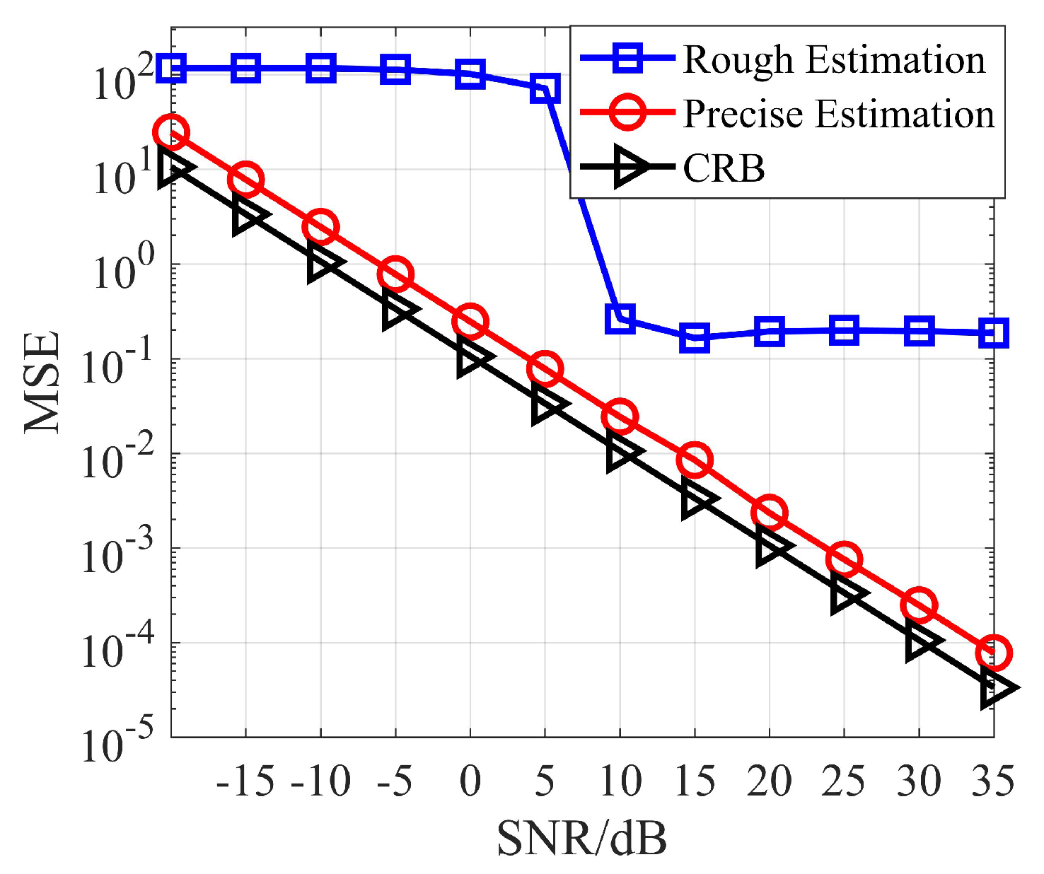
3.2. Rough Estimation

In order to obtain the RD frequency curve, the TF graph of ${\tilde{s}}_l\left(t\right)$ is obtained by the TF analysis. Considering the weak undulation of the RD frequency curve, the SPWVD function, which has relatively high TF resolution, is selected to extract the TF graph of ${\tilde{s}}_l\left(t\right)$. The RD frequency curve ${\hat{f}}_R\left(t\right)$ is obtained by extracting the ridge of SPWVD spectrum through the skeleton extraction method [13]. After that, the curve parameters $C_1\sim C_6$ are first estimated, and then the rough estimation of the micromotion parameters $\tilde{\mathbf{\eta }}$ are calculated.

According to the least squares (LS) criterion, the micromotion parameters estimation problem can be described as an optimization problem

$$\tilde{\mathbf{\eta }}=\underset{\mathbf{\eta }}{\mathrm{argmin}}{∥{\hat{f}}_R\left(t\right)-f_R\left(t,\mathbf{\eta }\right)∥}_2.$$

(20)

The RD frequency curve $f_R\left(t,\mathbf{\eta }\right)$, as shown in (16), is non-convex with respect to the micromotion parameters $\mathbf{\eta }$, meaning that convex optimization methods are unsuitable for this problem. In order to obtain a closed form solution of the vector $\mathbf{\eta }$, the rough estimation process includes two steps. In the first step, the RD frequency curve parameters $C_1\sim C_6$ are estimated, and then the micromotion parameters $\mathbf{\eta }$ are solved. For convenience in solving $C_1\sim C_6$, ${\hat{f}}_R\left(t\right)$ can be further simplified:

$$\frac{2\pi {\hat{f}}_R\left(t\right)}{l\omega }\left(C_3+C_{4}cos{\varphi }_t+C_{5}sin{\varphi }_t+C_{6}cos2{\varphi }_t\right)-C_{1}cos{\varphi }_t-C_{2}sin{\varphi }_t=1.$$

(21)

The initial phase $\gamma$ to be estimated is separated from ${\varphi }_t$, and (21) is rewritten as

$$\begin{array}{cc}\hfill H\times \xi & =\mathbf{1},\hfill \end{array}$$

(22)

where $\mathbf{1}$ represents the unit column vector of length m,

$$\begin{array}{cccc}\hfill H& ={\left[{\mathit{h}}_0,{\mathit{h}}_1,\cdots ,{\mathit{h}}_{N-1}\right]}^{\mathrm{T}}\hfill & \hfill {\mathit{h}}_i& =\left[\begin{array}{c}\frac{2\pi }{l\omega }{\hat{f}}_R\left(t_i\right)\\ \frac{2\pi }{l\omega }{\hat{f}}_R\left(t_i\right)cos\left(\omega t_i\right)\\ \frac{2\pi }{l\omega }{\hat{f}}_R\left(t_i\right)sin\left(\omega t_i\right)\\ \frac{2\pi }{l\omega }{\hat{f}}_R\left(t_i\right)cos\left(2\omega t_i\right)\\ \frac{2\pi }{l\omega }{\hat{f}}_R\left(t_i\right)sin\left(2\omega t_i\right)\\ cos\left(\omega t_i\right)\\ sin\left(\omega t_i\right)\end{array}\right]\xi =\left[\begin{array}{c}{C}_3\\ C_{4}cos\left(\gamma \right)+C_{5}sin\left(\gamma \right)\\ -C_{4}sin\left(\gamma \right)+C_{5}cos\left(\gamma \right)\\ C_{6}cos2\left(\gamma \right)\\ -C_{6}sin2\left(\gamma \right)\\ -C_{1}cos\left(\gamma \right)-C_{2}sin\left(\gamma \right)\\ C_{1}sin\left(\gamma \right)-C_{2}cos\left(\gamma \right)\end{array}\right],\hfill \end{array}$$

and m is the number of sampling points on ${\hat{f}}_R\left(t\right)$, $\xi$ is the intermediate variable. Then, the least squares estimation (LSE) of the intermediate variable $\xi$ can be obtained as

$$\begin{array}{c}\hfill \hat{\xi }={\left(H^{\mathrm{T}}H\right)}^{-1}{H}^{\mathrm{T}}\mathbf{1}\end{array}$$

(23)

And then, the initial phase $\gamma$ and the RD frequency curve parameters ${\hat{C}}_1\sim {\hat{C}}_6$ can be calculated by

$$\begin{array}{cccc}\hfill \hat{\gamma }& =0.5\mathrm{atan}\left({\hat{\xi }}_5/{\hat{\xi }}_4\right)\hfill & \hfill {\hat{C}}_1& =-{\hat{\xi }}_{6}cos\left(\hat{\gamma }\right)+{\hat{\xi }}_{7}sin\left(\hat{\gamma }\right)\hfill \\ \hfill {\hat{C}}_2& =-{\hat{\xi }}_{6}sin\left(\hat{\gamma }\right)-{\hat{\xi }}_{7}cos\left(\hat{\gamma }\right)\hfill & \hfill {\hat{C}}_3& ={\hat{\xi }}_1\hfill \\ \hfill {\hat{C}}_4& ={\hat{\xi }}_{2}cos\left(\hat{\gamma }\right)-{\hat{\xi }}_{3}sin\left(\hat{\gamma }\right)\hfill & \hfill {\hat{C}}_5& ={\hat{\xi }}_{2}sin\left(\hat{\gamma }\right)+{\hat{\xi }}_{3}cos\left(\hat{\gamma }\right)\hfill \\ \hfill {\hat{C}}_6& ={\hat{\xi }}_4/cos2\left(\hat{\gamma }\right)={\hat{\xi }}_5/sin2\left(\hat{\gamma }\right),\hfill \end{array}$$

(24)

where ${\hat{\xi }}_i$ represents the i-th element of the intermediate variable $\hat{\xi }$. Here, the estimations of RD frequency curve parameters ${\hat{C}}_1$∼${\hat{C}}_6$ and the Euler angle $\hat{\gamma }$ are obtained.

Substituting (24) into (16), the remaining micromotion parameters can be obtained by

$$\begin{array}{cc}\hfill {\hat{\phi }}_{\alpha }& =\mathrm{atan}(2{\hat{C}}_2/{\hat{C}}_4)=\mathrm{atan}({\hat{C}}_5/2{\hat{C}}_1)\hfill \end{array}$$

(25a)

$$\begin{array}{cc}\hfill \hat{\beta }& =\mathrm{atan}(\widehat{C_1}/2\widehat{C_4})=\mathrm{acos}({\hat{C}}_5/2{\hat{C}}_2)=-{\hat{C}}_6\pm \sqrt{1+{\hat{C}}_6^2}.\hfill \end{array}$$

(25b)

Substituting ${\hat{\phi }}_{\alpha },\hat{\beta },\hat{\gamma }$ into the RD frequency curve parameters ${\hat{C}}_1\sim {\hat{C}}_6$, the ratio ${\rho }_o/r_a$ of deflection distance and the rotation radius can be estimated. So far, the rough estimation $\tilde{\mathbf{\eta }}$ is performed. The bias of the SPWVD function leads to the deviation of the high frequency component of the RD frequency curve estimation result. Accordingly, the rough estimation $\tilde{\mathbf{\eta }}$ deviates from the true value of the micromotion parameters. However, the rough estimation $\tilde{\mathbf{\eta }}$ is only a priori of the accurate estimation, so it does not affect the final parameter estimated performance.

3.3. Precise Estimation

In this subsection, the MLE of the micromotion parameters $\mathbf{\eta }$ is analyzed. As discussed in [20], the MLE of $\mathbf{\eta }$ can be obtained by testing the likelihood ratio of a pair of hypotheses, where $H_1$ corresponds to the target existence hypothesis as in (19), and $H_0$ corresponds to the noise-only hypothesis. The likelihood ratio function is given by

$$\begin{array}{cc}\hfill \mathrm{\Lambda }& \left(\mathbf{\eta };{\tilde{s}}_l\left(t\right)\right)=e^{-\frac{1}{{\sigma }_n^2}{\int }_0^T{\left|{\tilde{s}}_l\left(t\right)-{\hat{\sigma }}_q{e}^{jl{\phi }_q\left(t\right)}\right|}^2\mathrm{d}t}.\hfill \end{array}$$

(26)

After logarithmic operation of (26), we can obtain ($\Re \left\{·\right\}$ represents the operation of taking the real part).

$$\begin{array}{cc}\hfill L\left(\mathbf{\eta };{\tilde{s}}_l\left(t\right)\right)& =ln\mathrm{\Lambda }\left(\mathbf{\eta };{\tilde{s}}_l\left(t\right)\right)\hfill \\ \hfill & =-\frac{1}{{\sigma }_n^2}{\int }_0^T{\left|{\tilde{s}}_l\left(t\right)-{\hat{\sigma }}_q{e}^{2jl{\phi }_q\left(t\right)}\right|}^2\mathrm{d}t\hfill \\ \hfill & =\frac{2{\hat{\sigma }}_q}{{\sigma }_n^2}{\int }_0^T\Re \left\{{\tilde{s}}_l\left(t\right)e^{-2jl{\phi }_q\left(t\right)}\right\}\mathrm{d}t+\mathrm{constant},\hfill \end{array}$$

(27)

where $\mathrm{constant}=-2{\hat{\sigma }}_q^{2}T/{\sigma }_n^2-2{\int }_0^T{\tilde{s}}_l\left(t\right){\tilde{s}}_l^{*}\left(t\right)\mathrm{d}t/{\sigma }_n^2$ is independent of the micromotion parameters $\mathbf{\eta }$. Thus, the MLE of $\mathbf{\eta }$ can be written as

$$\begin{array}{cc}\hfill {\hat{\mathbf{\eta }}}_{\mathrm{ML}}& =\underset{\mathbf{\eta }}{\mathrm{argmax}}L\left(\mathbf{\eta };{\tilde{s}}_l\left(t\right)\right)\hfill \\ \hfill & =\underset{\mathbf{\eta }}{\mathrm{argmax}}{\int }_0^T\Re \left\{{\tilde{s}}_l\left(t\right)e^{-2jl{\phi }_q\left(t\right)}\right\}\mathrm{d}t.\hfill \end{array}$$

(28)

No further simplification seems possible for the MLE from (28), and a four dimensional search is required for obtaining the MLE of $\mathbf{\eta }$ in (17) numerically. We utilize the PSO algorithm to optimize (28). The rough estimation $\tilde{\mathbf{\eta }}$ is used as the initial value of the PSO algorithm.

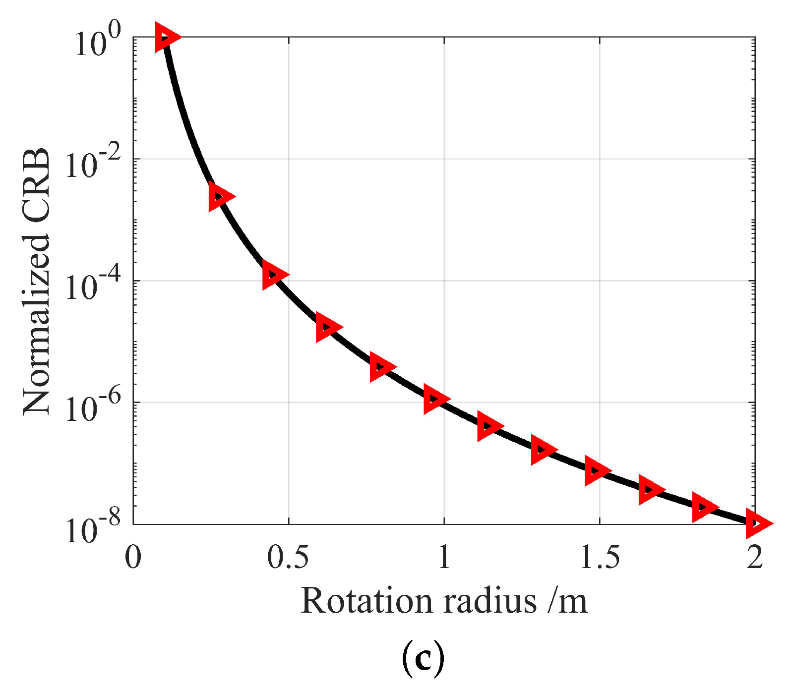
3.4. Performance Analysis

In this subsection, we provide the CRB for jointly estimating the micromotion parameters $\mathbf{\eta }$. The first step in obtaining the CRB is to compute the Fisher information matrix (FIM) $\mathbf{J}\left(\mathbf{\eta }\right)$, which is a $4\times 4$ matrix related to the second-order derivatives of the joint log-likelihood [21].

$$\begin{array}{cc}\hfill \mathbf{J}\left(\mathbf{\eta }\right)& =\mathrm{E}\left[\frac{{\partial }^{2}L\left(\mathbf{\eta };{\tilde{s}}_l\left(t\right)\right)}{\partial \mathbf{\eta }\partial {\mathbf{\eta }}^{\mathrm{T}}}\right]\hfill \\ \hfill & =\frac{2l^2{\left|{\sigma }_q\right|}^2}{{\sigma }_n^2}{\int }_T\frac{\partial {\phi }_q\left(t\right)}{\partial \mathbf{\eta }}\frac{\partial {\phi }_q\left(t\right)}{\partial {\mathbf{\eta }}^{\mathrm{T}}}\mathrm{d}t\hfill \\ \hfill & =2·\mathrm{SNR}{\int }_T\frac{\partial {\phi }_q\left(t\right)}{\partial \mathbf{\eta }}\frac{\partial {\phi }_q\left(t\right)}{\partial {\mathbf{\eta }}^{\mathrm{T}}}\mathrm{d}t\hfill \end{array},$$

(29)

where $\mathrm{SNR}=l^2·{\left|{\sigma }_q\right|}^2/{\sigma }_n^2$ represents the normalized signal-to-noise ratio (SNR). The main lobe gain of $l$-mode VEMW is approximately inversely proportional to $\left|l\right|$, so $l^2·{\left|{\sigma }_q\right|}^2/{\sigma }_n^2$ can be regarded as the normalized SNR. $\partial {\phi }_q\left(t\right)/\partial \mathbf{\eta }$ is the partial derivative of ${\phi }_q\left(t\right)$ with respect to the micromotion parameters $\mathbf{\eta }$, as given by

$$\begin{array}{cc}\hfill \frac{\partial {\phi }_q\left(t\right)}{\partial \mathbf{\eta }}& =\frac{1}{{\mathrm{\Xi }}_t}·\left[\begin{array}{c}(-1+{sin}^2\beta {sin}^2{\varphi }_t-\frac{{\rho }_o}{r_a}cos{\phi }_{\alpha }cos{\varphi }_t-\frac{{\rho }_o}{r_a}sin{\phi }_{\alpha }cos\beta sin{\varphi }_t)\\ \left(-sin\beta sin{\varphi }_{t}cos{\varphi }_t-\frac{{\rho }_o}{r_a}cos{\phi }_{\alpha }sin\beta sin{\varphi }_t\right)\\ \left(cos\beta +\frac{{\rho }_o}{r_a}sin{\phi }_{\alpha }sin{\varphi }_t+\frac{{\rho }_o}{r_a}cos{\phi }_{\alpha }cos\beta cos{\varphi }_t\right)\\ \left(-sin{\phi }_{\alpha }cos{\varphi }_t+cos{\phi }_{\alpha }cos\beta sin{\varphi }_t\right)\end{array}\right]\hfill \\ \hfill {\mathrm{\Xi }}_t& =1-{sin}^2\beta {sin}^2{\varphi }_t+\frac{{\rho }_o^2}{r_a^2}+\frac{2{\rho }_o}{r_a}cos{\phi }_{\alpha }cos{\varphi }_t+\frac{2{\rho }_o}{r_a}sin{\phi }_{\alpha }cos\beta sin{\varphi }_t\hfill \end{array}.$$

(30)

The CRB of the each micromotion parameters in $\mathbf{\eta }$ are determined by the diagonal elements of ${\mathbf{J}}^{-1}\left(\mathbf{\eta }\right)$.

$$\begin{array}{cccc}\hfill \mathrm{var}\left(\hat{\phi }\right)& \ge {\left[{\mathbf{J}}^{-1}\left(\mathbf{\eta }\right)\right]}_{1,1},\hfill & \hfill \mathrm{var}\left(\hat{\beta }\right)& \ge {\left[{\mathbf{J}}^{-1}\left(\mathbf{\eta }\right)\right]}_{2,2},\hfill \\ \hfill \mathrm{var}\left(\hat{\gamma }\right)& \ge {\left[{\mathbf{J}}^{-1}\left(\mathbf{\eta }\right)\right]}_{3,3},\hfill & \hfill \mathrm{var}\left(\widehat{\frac{{\rho }_o}{r_a}}\right)& \ge {\left[{\mathbf{J}}^{-1}\left(\mathbf{\eta }\right)\right]}_{4,4},\hfill \end{array}$$

(31)

where $\mathrm{var}\left(·\right)$ represents the variance. For any nonsingular FIM, a closed-form expression for the CRB can be easily obtained (though we are not going to write down the lengthy formula here), since the analytical form of ${\mathbf{J}}^{-1}\left(\mathbf{\eta }\right)$ can be easily derived from (29) using Cramer’s rule. The CRB for the micromotion parameters $\mathbf{\eta }$ can be written as

$$\begin{array}{ccc}\hfill \mathrm{CRB}=& {\left[{\mathbf{J}}^{-1}\left(\mathbf{\eta }\right)\right]}_{1,1}+{\left[{\mathbf{J}}^{-1}\left(\mathbf{\eta }\right)\right]}_{2,2}+\hfill & \hfill {\left[{\mathbf{J}}^{-1}\left(\mathbf{\eta }\right)\right]}_{3,3}+{\left[{\mathbf{J}}^{-1}\left(\mathbf{\eta }\right)\right]}_{4,4}.\end{array}$$

(32)

The CRB corresponds to the azimuth curve of the scattering point q, that is, it is related to the true value of the parameter. Therefore, the simulation section investigates the parameter estimated performance under different rotation states.

4. Simulation Results and Analysis

In this section, groups of simulations are presented to validate the correctness of the above-mentioned theoretical analyses.

4.1. Effectiveness Analysis

The geometry of the UCA radar and the rotating scattering point q is same as Figure 1 in the simulation. Through numerical simulations, we analyze the performance of the above algorithm and compare the rough estimation $\tilde{\eta }$ and MLE ${\hat{\eta }}_{\mathrm{ML}}$ of the micromotion parameters with the CRB. The detailed derivation of the CRB expressions is presented in Section 3.4. In order to obtain an abundant TF resolution of the SPWVD spectrum of rotating target, the angular frequency is set as $10\pi$ rad/s. The other simulation parameters are listed in

Table 1. Key parameters in the simulation.

Parameter	Value
Carrier frequency	10 GHz
Wavelength	0.03 m
Aperture of the front	0.09 m
Coherent accumulation time	2 s
PRF	1 kHz
Vortex mode	3
Angular velocity	10$\pi$ rad/s
Rotation radius	1 m
Euler angle	$({40}^{\circ },{30}^{\circ },0^{\circ })$
Coordinates of o	(4.5 m, 0 m, 20 m${)}^{\mathrm{T}}$

. It is worth mentioning that considering the dynamic change of ${\phi }_q\left(t\right)$, we set the $Z_o$ as 20 m. For the long-distance target, the scene can be enlarged according to the scaled model.

For the rough estimation $\tilde{\mathbf{\eta }}$, the TF curve ${\hat{f}}_R\left(t\right)$ of q is estimated firstly. Figure 4 shows the SPWVD spectrum and the extracted TF curve of the scattering point q. The black line represents the theoretical RD frequency curve. The red line represents the extracted TF curve ${\hat{f}}_R\left(t\right)$. It can be found that the TF curve ${\hat{f}}_R\left(t\right)$ is almost consistent with the theoretical RD frequency curve except the valley bottoms. The deviation at the valley bottom is due to the bias of SPWVD. The green line in Figure 4b represents the distance from the rotation trajectory to the VEMW axis. Near the trough where the instantaneous frequency estimation deviates from the theoretical RD frequency, the deflection distance of the rotation trajectory reaches the minimum value, which is the point where the target is closest to the VEMW axis during the rotatio. The reason is that, not strictly speaking, SPWVD function is regarded as the Fourier transform of the instantaneous autocorrelation function of the signal. When the local stability of the signal is weak, such as the valley of ${\hat{f}}_R\left(t\right)$ shown in Figure 4b, SPWVD method cannot accurately capture subtle changes. However, for different signals, we can adjust the shape of smooth window of SPWVD to make the value of valley closer to the theoretical curve. In addition, SPWVD method has boundary effect, that is, spectrum at the beginning and end of the signal cannot reflect the real TF characteristics. The instantaneous frequency estimation deviates from the true value. So the SPWVD spectrum near the accumulation time boundary needs to be ignored. After extracting the RD frequency curve, the estimation results of the curve parameters ${\hat{C}}_1\sim {\hat{C}}_6$ based on (23) and (24) are as shown in

Table 2. Estimation results of the RD frequency curve parameters.

Parameter	${\mathit{C}}_1$	${\mathit{C}}_2$	${\mathit{C}}_3$	${\mathit{C}}_4$	${\mathit{C}}_5$	${\mathit{C}}_6$
Theoretical Value	3.50	−3.39	25.16	8.09	−5.88	0.14
Estimated Value	4.23	−3.71	29.77	8.39	−5.49	0.23

, which shows that the estimated results of the curve parameters are close to the theoretical values.

Table 3. Estimation results of micromotion parameters.

Parameter	${\mathit{\phi }}_{\mathit{\alpha }}$	$\mathit{\beta }$	$\mathit{\gamma }$	${\mathit{\rho }}_{\mathit{o}}/{\mathit{r}}_{\mathit{a}}$
Theoretical Value	−0.70 rad	0.52 rad	0 rad	4.57
Rough Estimated Value	−0.72 rad	0.49 rad	0.06 rad	4.87
Precise Estimated Value	−0.70 rad	0.52 rad	0.00 rad	4.57

shows the estimation results of micromotion parameters. Using the estimated RD curve parameters ${\hat{C}}_1\sim {\hat{C}}_6$, the estimated value of $\tilde{\mathbf{\eta }}$ is shown in the second row, which is close to the theoretical value, corresponding to the first row. Based on the rough estimation $\tilde{\mathbf{\eta }}$ calculated from the extracted TF curve ${\hat{f}}_R\left(t\right)$, the MLE ${\hat{\mathbf{\eta }}}_{\mathrm{ML}}$ of the micromotion parameters is calculated, corresponds to the third row. According to Table 3, the average estimation error of the precise estimation ${\hat{\mathbf{\eta }}}_{\mathrm{ML}}$ is 0.06%. This shows that the two-step micromotion parameters estimation method for a rotating target based on VEMW proposed in this paper can realize the effective estimation of micromotion parameters $\mathbf{\eta }$.

In addition, we conducted experimental verification. The experimental parameter settings are shown in

Table 4. The parameters of the corner reflector.

Parameter	Value
Carrier frequency	35 GHz
Bandwidth	110 MHz
Pulse width	50 $\mathsf{\mu }$s
PRF	500 Hz
Rotation radius	0.2 m
Coordinate of o	${(0.1,0,5)}^{\mathrm{T}}$m
Euler angle	$({40}^{\circ },{30}^{\circ },0^{\circ })$
Angular velocity	10$\pi$ rad/s

, and the experimental scenario is shown in Figure 5. A corner reflector is selected as the point target in the experiment. Figure 6a of the response shows the SPWVD spectrum of the blade. Figure 6b shows the theoretical and extracted TF curves.

Table 5. Estimation results of micromotion parameters (corner reflector).

Parameter	${\mathit{\phi }}_{\mathit{\alpha }}$	$\mathit{\beta }$	$\mathit{\gamma }$	${\mathit{\rho }}_{\mathit{o}}/{\mathit{r}}_{\mathit{a}}$
Theoretical Value	0.6981 rad	0.5236 rad	0 rad	0.5
Rough Estimated Value	0.5483 rad	0.4877 rad	0.1628 rad	0.4726
Precise Estimated Value	0.6981 rad	0.5236 rad	0 rad	0.5

shows the parameter estimation result of the rotating corner reflector which verified the effectiveness of the algorithm.

Since radar works in a noisy environment, the robustness of the algorithm to noise is demonstrated. In this section, the complex Gaussian white noise is added to the signal. We calculated the MSE of the parameters to evaluate the performance of the proposed method. The MSE of the micromotion parameters $\mathbf{\eta }$ are obtained with 1000 Monte Carlo experiments, which is expressed as

$$\mathrm{MSE}=\frac{1}{1000}\sum _{i=1}^{1000}{\parallel {\hat{\mathbf{\eta }}}_i-\mathbf{\eta }\parallel }_2^2,$$

(33)

Figure 7 shows the estimation performance of the proposed two-step method under different SNRs. The input SNR here refers to the normalized SNR as (29). The line with asterisk, circle, and trigonometry markers represent the rough estimation $\tilde{\mathbf{\eta }}$, the precise estimation ${\hat{\mathbf{\eta }}}_{\mathrm{ML}}$, and the CRB of the micromotion parameters $\mathbf{\eta }$. Rough estimation $\tilde{\mathbf{\eta }}$ are far away from CRB. When the SNR is less than 5dB, the MSE of rough estimation $\tilde{\mathbf{\eta }}$ is large. This is because the RD frequency curve of the target is submerged in the noise environment, so that the RD curve parameters ${\hat{C}}_1\sim {\hat{C}}_6$ cannot be effectively estimated. As a consequence, the effective estimation of the micromotion parameters $\tilde{\mathbf{\eta }}$ cannot be obtained. When the SNR is greater than or equal to the 5dB, the MSE of the rough estimation $\tilde{\mathbf{\eta }}$ decreases with the increase of the SNR and approaches the CRB. Precision estimation measures correct the bias of rough estimation by designing objective functions in the signal domain instead of estimating parameters in the TF domains. For precise estimation, the rough estimation is only used as prior knowledge to improve the efficiency of the PSO algorithm and does not affect the performance of the final precise estimation. As shown in Figure 7, a threshold phenomenon exists for the MSE of the rough estimation $\tilde{\mathbf{\eta }}$. When the SNR is greater than 10 dB, the MSE of rough estimation remains at a stable value instead of increasing with the SNR and closing to the CRB, which comes from the bias of SPWVD spectrum. The value of the 10 dB threshold is related to the ratio of the angular frequency $\omega$ to the PRF, which will be analyzed in Section 4.2. The MSE of precise estimation ${\hat{\mathbf{\eta }}}_{\mathrm{ML}}$ is close to CRB in the dynamic range of SNR. Above all, numerical simulations verify the effectiveness of the proposed algorithm in the noise environment.

4.2. Effect Analysis of True Value of the Micromotion Parameter

The above subsection has verified the effectiveness of the algorithm for estimation of micromotion parameters. In this subsection, the influence factors of estimation performance are analyzed. As mentioned at the end of Section 3.4, CRB is affected by the true value of micromotion parameters $\mathbf{\eta }$ except $\gamma$ due to integral effect. Therefore, we analyse the estimation performance with different micromotion parameters, including three groups of experiments:

• angular frequency $\omega$;
• ratio of deflection distance to radius of rotation ${\rho }_o/r_a$;
• rotating attitude ${\phi }_{\alpha },\beta$.

4.2.1. Angular Frequency

The resolution in the frequency domain depends on the accumulation time T, while the resolution in the time domain depends on the PRF. When these two parameters are determined, the angular frequency $\omega$ will affect the characteristics of the extracted TF curve ${\hat{f}}_R\left(t\right)$ both the fluctuation and the amplitude, which in turn affect the rough estimation $\tilde{\mathbf{\eta }}$. Therefore, especially for the rough estimation $\tilde{\mathbf{\eta }}$ based on the extracted TF curve ${\hat{f}}_R\left(t\right)$, it is necessary to analyze the influence of angular frequency $\omega$. We set three values of angular frequency: $\omega =5\pi$ rad/s, $\omega =10\pi$ rad/s, $\omega =15\pi$ rad/s, whose rough estimations correspond to the purple line, brown line and blue line of Figure 8, respectively. According to the characteristics of the TF curve, we discuss the impact of angular frequencies at high SNRs. When the SNR is greater than 20 dB, the lower the angular frequency $\omega$, the more accurate the rough estimation $\tilde{\mathbf{\eta }}$ of the micromotion parameters. The integral operation used in (29) eliminates the influence of the angular frequency $\omega$ on the CRB. Therefore, the precise estimation ${\hat{\mathbf{\eta }}}_{\mathrm{ML}}$ and CRB of micromotion parameters remain unchanged at different angular frequencies.

4.2.2. Ratio of Deflection Distance to Radius of Rotation

We fix the deflection distance ${\rho }_o$ and change the rotation radius $r_a$ to investigate the effect of the ratio ${\rho }_o/r_a$ on the parameter estimated performance. Except for the Figure 7 with fixed rotation radius of 1 m, we set the control simulation with rotation radii of 0.8 m and 0.5 m corresponding to the Figure 9a and Figure 9b, respectively. The rotation radius $r_a$ affects the performance of the rough estimation $\tilde{\mathbf{\eta }}$. The small rotation radius makes the rough estimation bias larger at low SNR and makes the SNR threshold larger. When $r_a=0.5\mathrm{m}$, the SNR threshold is 35 dB. When $r_a=0.8\mathrm{m}$, the SNR threshold is 15 dB. However, under different rotation radii, the steady-state deviation is similar when the SNR is greater than the threshold. In addition, the rotation radius $r_a$ affects the CRB of parameter estimation. Taking the same SNR, the CRB is the smallest when the rotation radius is 1 m, followed by 0.8 m, and the largest is 0.5 m. At different rotation radii, the precise estimations are always close to CRB. Figure 10a shows the normalized result of CRB when the rotation radius changes continuously from 0.1 m to 2 m. The larger the rotation radius, the better the theoretical estimated performance of ${\hat{\mathbf{\eta }}}_{\mathrm{ML}}$. From the point of view of physical concept, the fundamental reason is that the large rotation radius corresponds to obvious azimuth change which leads to good parameter estimated performance.

4.2.3. Rotating Attitude

Since the azimuth of rotation center ${\phi }_o$ appears jointly with $\alpha$ in CRB as (30), it is set as 0 to simplify the numerical analysis and only explore the influence of $(\alpha ,\beta )$ which corresponds to the rotation attitude. Physically speaking, the omission of the azimuth of rotation center ${\phi }_o$ only corresponds to different initial states, and does not affect the analysis of estimated performance. The RD effect essentially utilize the change of the azimuth. Different $(\alpha ,\beta )$ correspond to the target cutting the isophase surface of the VEMW with different angular frequencies and attitudes. We select four rotation attitudes for analysis, which are ${(\alpha ,\beta ,\gamma )}_1=({40}^{\circ },{30}^{\circ },0^{\circ })$, ${(\alpha ,\beta ,\gamma )}_2=(0^{\circ },0^{\circ },0^{\circ })$, ${(\alpha ,\beta ,\gamma )}_3=({90}^{\circ },{90}^{\circ },0^{\circ })$, ${(\alpha ,\beta ,\gamma )}_4=(0^{\circ },{90}^{\circ },0^{\circ })$, respectively. The corresponding rotation trajectories are shown in Figure 10. The lower figure of each subfigure in Figure 10 represents the projection of the rotation trajectory on the $XOY$ plane. The rough estimation $\tilde{\mathbf{\eta }}$, precise estimation ${\hat{\mathbf{\eta }}}_{\mathrm{ML}}$ and CRB results of ${(\alpha ,\beta ,\gamma )}_1$ are shown in Figure 7. The corresponding results of ${(\alpha ,\beta ,\gamma )}_2$ and ${(\alpha ,\beta ,\gamma )}_3$ are shown in Figure 11, where the red line represents the result of ${(\alpha ,\beta ,\gamma )}_2$ and the black line represents the result of ${(\alpha ,\beta ,\gamma )}_3$. As show in Figure 10b, when the Euler angle is ${(\alpha ,\beta ,\gamma )}_4=(0^{\circ },{90}^{\circ },0^{\circ })$, the azimuth angle ${\phi }_q\left(t\right)$ of the rotating target does not change during the rotation, so the rotating Doppler frequency is always 0. Comparing Figure 7 and Figure 11, it can be found that the steady-state performances of the rough estimation results corresponding to different rotation attitudes are different, where ${(\alpha ,\beta ,\gamma )}_2$ is the best, ${(\alpha ,\beta ,\gamma )}_1$ is the second, and ${(\alpha ,\beta ,\gamma )}_3$ is the worst. At the same SNR, the CRB of micromotion parameters $\mathbf{\eta }$ corresponding to different rotation attitudes are also different. Different from the rough estimation $\tilde{\mathbf{\eta }}$, the CRB of ${(\alpha ,\beta ,\gamma )}_3$ is the smallest, and that of ${(\alpha ,\beta ,\gamma )}_1$ and ${(\alpha ,\beta ,\gamma )}_2$ are almost the same. The precise estimation ${\hat{\mathbf{\eta }}}_{\mathrm{ML}}$ is always close to CRB.

Subsequently, we investigate the influence of $\alpha$ and $\beta$ involving all rotational attitudes on the performance of parameter estimation, as shown in Figure 12a. The dynamic range of $\alpha$ and $\beta$ are set as 0${}^{\circ }$ to 90${}^{\circ }$. Since the variation range of CRB is tremendous, the negative natural logarithm of CRB is set as the vertical coordinate to facilitate observation. The larger the vertical coordinate is, the better the precise performance of parameter estimation is. Figure 12a shows that CRB reaches minimum at $\beta =0^{\circ }$ for all $\alpha$, while the rotation plane is parallel to $XOY$ plane. When $(\alpha ,\beta )=(0^{\circ },{90}^{\circ })$, the CRB reaches a maximum, while the rotation plane is vertical to the array and parallel to $XOZ$ plane. The azimuth angle ${\phi }_q\left(t\right)$ of rotating target does not change during the rotation, so the micromotion parameters $\mathbf{\eta }$ cannot be estimated based on the RD effect. Other situations fall between the above two extremes. In addition, we select some cross sections of the performance surface shown in Figure 12a to observe the change of CRB with fixed $\beta$ under different $\alpha$, as shown in Figure 12b. For $\alpha =0^{\circ },{40}^{\circ }$ and ${90}^{\circ }$, the CRB reaches a minimum at $\beta =0^{\circ }$, and as $\beta$ increases, the CRB becomes larger. When $\left(\alpha ,\beta \right)$ is close to $(0^{\circ },{90}^{\circ })$, the parameter estimation gradually fails. Finally, we select some cross sections of the performance surface shown in Figure 12a to observe the change of CRB with fixed $\alpha$ under different $\beta$, as shown in Figure 12c. It can be seen that the performance of micromotion parameters estimation is optimal when the rotation plane is parallel to the $XOY$ plane. When $\beta ={40}^{\circ }$, the CRB does not change significantly with the $\alpha$, which may be because the projection position and shape of the rotation trajectory on the $XOY$ plane remain unchanged. When the tilt angle $\beta ={90}^{\circ }$, CRB decreases with the increase of $\alpha$, and reaches the optimum at $\alpha ={90}^{\circ }$, but it is still worse than the previous two cases. In summary, the performance of micromotion parameters estimation is related to the projection position and shape of the rotation trajectory on the $XOY$ plane.

5. Conclusions

In this paper, we studied the estimated performance of micromotion parameters in the case of unavailable rotation center position in VEMW radar system. Firstly, we analyzed the parameters that can be extracted from the RD effect when the rotation center position is unknown. Then, we proposed a two-step estimation algorithm for the micromotion parameters which is verified by simulation and experiment. The first step is based on the SPWVD spectrum, and the rough estimation of the micromotion parameters is obtained according to the extracted TF curve parameters. Due to the bias of SPWVD, the second step is to optimize the likelihood ratio function based on PSO algorithm to correct the rough estimation and obtain the precise estimation. Finally, we derived the CRB of the micromotion parameters. The analysis shows that the true value of the micromotion parameters affect the performance of the parameter estimation, which is verified in the simulation part. Furthermore, the simulation results show that the two-step parameter estimation algorithm can achieve CRB. In the next step, we will utilize the multi-modal information to estimate the accurate position of the rotation center and provide new information for the detection of rotating objects in complex backgrounds.

References

1. Allen, L.; Beijersbergen, M.W.; Spreeuw, R.; Woerdman, J. Orbital angular momentum of light and the transformation of Laguerre–Gaussian laser modes. Phys. Rev. A 1992, 45, 8185. [Google Scholar] [CrossRef] [PubMed]
2. Nienhuis, G. Doppler effect induced by rotating lenses. Opt. Commun. 1996, 132, 8–14. [Google Scholar] [CrossRef]
3. Bialynicki-Birula, I.; Bialynicka-Birula, Z. Rotational frequency shift. Phys. Rev. Lett. 1997, 78, 2539. [Google Scholar] [CrossRef]
4. Courtial, J.; Dholakia, K.; Robertson, D.; Allen, L.; Padgett, M. Measurement of the rotational frequency shift imparted to a rotating light beam possessing orbital angular momentum. Phys. Rev. Lett. 1998, 80, 3217. [Google Scholar] [CrossRef]
5. Lavery, M.P.; Speirits, F.C.; Barnett, S.M.; Padgett, M.J. Detection of a spinning object using light’s orbital angular momentum. Science 2013, 341, 537–540. [Google Scholar] [CrossRef] [PubMed]
6. Wang, L.; Tao, L.; Li, Z.; Wu, J.; Yang, J. Three dimensional electromagnetic vortex radar imaging based on the modified RD algorithm. In Proceedings of the IEEE Radar Conference (RadarConf20), Florence, Italy, 21–25 September 2020; pp. 1–5. [Google Scholar]
7. Bu, L.; Zhu, Y.; Chen, Y.; Yang, Y.; Zang, Y. Vortex-electromagnetic-wave-based ISAR imaging for high-speed maneuvering targets. Sci. Rep. 2022, 12, 18009. [Google Scholar] [CrossRef] [PubMed]
8. Zhao, M.; Gao, X.; Xie, M.; Zhai, W.; Xu, W.; Huang, S.; Gu, W. Measurement of the rotational Doppler frequency shift of a spinning object using a radio frequency orbital angular momentum beam. Opt. Lett. 2016, 41, 2549–2552. [Google Scholar] [CrossRef] [PubMed]
9. Zhou, Z.; Cheng, Y.; Liu, K.; Liu, H. Detection of uniformly accelerated spinning target based on OAM beams. In Proceedings of the International Conference on Microwave and Millimeter Wave Technology (ICMMT), Chengdu, China, 7–11 May 2018; pp. 1–3. [Google Scholar]
10. Brousseau, C.; Mahdjoubi, K.; Emile, O. Measurement of the rotational sense and velocity of an object using OAM wave in the radio-frequency band. Electron. Lett. 2019, 55, 709–711. [Google Scholar] [CrossRef]
11. Zheng, J.; Zheng, S.; Shao, Z.; Zhang, X. Analysis of rotational Doppler effect based on radio waves carrying orbital angular momentum. J. Appl. Phys. 2018, 124, 164907. [Google Scholar] [CrossRef]
12. Luo, Y.; Chen, Y.J.; Zhu, Y.Z.; Li, W.Y.; Zhang, Q. Doppler effect and micro-Doppler effect of vortex-electromagnetic-wave-based radar. IET Radar Sonar Navig. 2020, 14, 2–9. [Google Scholar] [CrossRef]
13. Wang, Y.; Liu, K.; Liu, H.; Wang, J.; Cheng, Y. Detection of rotational object in arbitrary position using vortex electromagnetic waves. IEEE Sensors J. 2020, 21, 4989–4994. [Google Scholar] [CrossRef]
14. Yuan, H.; Luo, Y.; Chen, Y.J.; Liang, J.; Liu, Y.X. Micro-motion parameter extraction of rotating target based on vortex electromagnetic wave radar. IET Radar Sonar Navig. 2021, 15, 1594–1606. [Google Scholar] [CrossRef]
15. Bu, L.; Zhu, Y.; Chen, Y.; Song, X.; Yang, Y.; Zang, Y. Micro-Motion Parameter Extraction of Multi-Scattering-Point Target Based on Vortex Electromagnetic Wave Radar. Remote Sens. 2022, 14, 5908. [Google Scholar] [CrossRef]
16. Wang, Z.; Luo, Y.; Li, K.; Yuan, H.; Zhang, Q. Micro-Doppler Parameters Extraction of Precession Cone-Shaped Targets Based on Rotating Antenna. Remote Sens. 2022, 14, 2549. [Google Scholar] [CrossRef]
17. Wang, Z.; Chen, Y.; Yuan, H.; Luo, Y.; Zhang, Q. Real Micro-Doppler Parameters Extraction of Spinning Targets Based on Rotating Interference Antenna. Remote Sens. 2022, 14, 5300. [Google Scholar] [CrossRef]
18. Liu, K.; Liu, H.; Qin, Y.; Cheng, Y.; Wang, S.; Li, X.; Wang, H. Generation of OAM beams using phased array in the microwave band. IEEE Trans. Antennas Propag. 2016, 64, 3850–3857. [Google Scholar] [CrossRef]
19. Chen, V.C.; Li, F.; Ho, S.S.; Wechsler, H. Micro-Doppler effect in radar: Phenomenon, model, and simulation study. IEEE Trans. Aerosp. Electron. Syst. 2006, 42, 2–21. [Google Scholar] [CrossRef]
20. Van Trees, H. Detection, Estimation, and Modulation Theory. Part 3, Radar-Sonar Signal Processing and Gaussian Signals in Noise; John Wiley & Sons: New York, NY, USA, 2001. [Google Scholar]
21. Sorenson, H.W. Parameter Estimation: Principles and Problems; Marcel Dekker Inc.: New York, NY, USA, 1980; Volume 9. [Google Scholar]
Figure 1. Observation model. (a) Geometry of uniform circular array (UCA) radar and a rotational target. (b) Euler angle ( α , β , γ ) between the reference coordinate system o X Y Z and the target-local coordinate system o x y z .
Remotesensing 15 02847 g001
Figure 2. Phase−front distribution of VEMW in a certain plane parallel to X O Y plane with centre located at Z-axis.
Remotesensing 15 02847 g002
Figure 3. The flowchart of the two-step micromotion parameters estimation method.
Remotesensing 15 02847 g003
Figure 4. Rotational Doppler effet. (a) TF image of the received signal. (b) Rotational Doppler frequency curve.
Remotesensing 15 02847 g004
Figure 5. The experiment scenario.
Remotesensing 15 02847 g005
Figure 6. Rotational Doppler effet of corner reflector. (a) SPWVD spectrum. (b) Theoretical and extracted TF curve.
Remotesensing 15 02847 g006aRemotesensing 15 02847 g006b
Figure 7. MSE vs. SNRs of m-D parameter η .
Remotesensing 15 02847 g007
Figure 8. MSE vs. SNRs of m-D parameter η with different angular frequencies.
Remotesensing 15 02847 g008
Figure 9. MSE vs. SNRs of m-D parameter η with different rotation radii. (a) r a = 0.8 m. (b) r a = 0.5 m. (c) CRB vs. rotation radii r a .
Remotesensing 15 02847 g009aRemotesensing 15 02847 g009b
Figure 10. The rotation trajectory of P with different Euler angles (left figure of each subfigure) and the corresponding projection of the motion trajectory on the X O Y plane (right figure of each subfigure). (a) ( α , β , γ ) 1 = ( 40 , 30 , 0 ) , (b) ( α , β , γ ) 2 = ( 0 , 0 , 0 ) , (c) ( α , β , γ ) 3 = ( 90 , 90 , 0 ) , (d) ( α , β , γ ) 4 = ( 0 , 90 , 0 ) .
Remotesensing 15 02847 g010
Figure 11. MSE vs. SNRs of m-D parameter η with different rotation attitudes. (The red line represents the result of ( α , β , γ ) 2 and the black line represents the result of ( α , β , γ ) 3 .)
Remotesensing 15 02847 g011
Figure 12. CRB performance surface of m-D parameter η versus rotation attitudes. (a) CRB performance surface vs. α , β . (b) CRB performance surface vs. β with different α . (c) CRB performance surface vs. α with different β .
Remotesensing 15 02847 g012