Article

A Thorough Evaluation of 127 Potential Evapotranspiration Models in Two Mediterranean Urban Green Sites

by
Nikolaos Proutsos
1,*,
Dimitris Tigkas
2,
Irida Tsevreni
3,
Stavros G. Alexandris
4,
Alexandra D. Solomou
1,
Athanassios Bourletsikas
1,
Stefanos Stefanidis
5 and
Samuel Chukwujindu Nwokolo
6
1
Institute of Mediterranean Forest Ecosystems-Hellenic Agricultural Organization “DEMETER”, Terma Alkmanos, 11528 Athens, Greece
2
Centre for the Assessment of Natural Hazards and Proactive Planning & Laboratory of Reclamation Works and Water Resources Management, National Technical University of Athens, 15780 Athens, Greece
3
Department of Early Childhood Education, University of Thessaly, 38221 Volos, Greece
4
Department of Natural Resources Development and Agricultural Engineering, Agricultural University of Athens, 11855 Athens, Greece
5
Laboratory of Mountainous Water Management and Control, School of Forestry and Natural Environment, Aristotle University of Thessaloniki, 54124 Thessaloniki, Greece
6
Department of Physics, Faculty of Physical Sciences, University of Calabar, Calabar 540004, Nigeria
*
Author to whom correspondence should be addressed.
Remote Sens. 2023, 15(14), 3680; https://doi.org/10.3390/rs15143680
Submission received: 15 June 2023 / Revised: 12 July 2023 / Accepted: 21 July 2023 / Published: 23 July 2023

Abstract

:
Potential evapotranspiration (PET) is a particularly important parameter for understanding water interactions and balance in ecosystems, while it is also crucial for assessing vegetation water requirements. The accurate estimation of PET is typically data demanding, while specific climatic, geographical and local factors may further complicate this task. Especially in city environments, where built-up structures may highly influence the micrometeorological conditions and urban green sites may occupy limited spaces, the selection of proper PET estimation approaches is critical, considering also data availability issues. In this study, a wide variety of empirical PET methods were evaluated against the FAO56 Penman–Monteith benchmark method in the environment of two Mediterranean urban green sites in Greece, aiming to investigate their accuracy and suitability under specific local conditions. The methods under evaluation cover all the range of empirical PET estimations: namely, mass transfer-based, temperature-based, radiation-based, and combination approaches, including 112 methods. Furthermore, 15 locally calibrated and adjusted models have been developed based on the general forms of the mass transfer, temperature, and radiation equations, improving the performance of the original models for local application. Among the 127 (112 original and 15 adjusted) evaluated methods, the radiation-based methods and adjusted models performed overall better than the temperature-based and the mass transfer methods, whereas the data-demanding combination methods received the highest ranking scores. The adjusted models seem to give accurate PET estimates for local use, while they might be applied in sites with similar conditions after proper validation.

1. Introduction

Evapotranspiration (ET) is a key component of the water cycle, while in rainfed ecosystems, it is the main consumer of available precipitation water [1,2,3]. The anticipated climate trends suggest that the magnitude of ET will increase due to warming and changing precipitation patterns impacting the earth’s ecosystems [4]. Due to its significance, accurate measurements or estimates of ET are crucial. However, direct ET measurement by methods such as lysimeters [5] or eddy covariance [6,7] is difficult to obtain due to the high requirements of expensive equipment or application difficulties. The estimation of ET by common meteorological data is generally acceptable, since it is easier and in many cases produces reliable estimates.
The site-specific characteristics highly influence the ET magnitudes. Thus, numerous estimation models have been proposed worldwide with different approaches, whereas the substrate at each site highly influences the ET rates [8]. In general, four major groups of methods can be defined to classify the empirical ET models: the mass-transfer-based methods, the temperature-based methods, the radiation-based methods and the combination methods. In all cases, the proposed equations aim to provide reliable estimates of the water demand driven by atmospheric conditions by minimizing the impact of plant species, vegetation stage or soil. To accomplish this, the estimates of ET are generally mentioned as potential (PET) or reference evapotranspiration, which are two different terms for expressing the water demand with different conceptual physical bases. The selection of the appropriate PET method is particularly important as it affects hydrometeorological and climatic variables that are linked to the sustainability of natural ecosystems [9].
Raza et al. [10] performed a comprehensive review on studies using several empirical evapotranspiration models and found that Thornthwaites’ 1948 and Hargreaves–Samani’s 1985 models were the most widely used among the temperature-based models, whereas Priestley 1972 and Ritchie 1972 were also the most often used among the radiation-based ones. However, the Penman–Monteith model is the most widely used in all categories.
The Penman–Monteith model is generally accepted as the most accurate method to estimate maximum ET as also suggested by the FAO (Food and Agriculture Organization of the United Nations) and WMO (World Meteorological Organization). In many studies, FAO56-PM is used as the standard method to compare and evaluate the performance of other methods in specific sites, areas or regions [11,12,13,14,15,16,17]. The FAO adopted the concept of reference evapotranspiration in the FAO guidelines for crop water requirements by Doorenbos and Pruitt [18,19]. This approach to calculating crop evapotranspiration is widely accepted by engineers, agronomists and researchers in practice, design and research. The reference concept relates to a growing reference grass crop and is represented in FAO-24 by climate types calibrated with lysimeter data from various locations [20]. However, many have pointed to weaknesses in the FAO-24 methodologies for implementation on a global scale. Researchers have tried to improve the evapotranspiration estimations for different locations and data availability through experimental and theoretical studies. First, the correlation of the calculated crop evapotranspiration with a reference crop proved difficult. The definition of a grass variety and its morphological characteristics have not been standardized for different climatic conditions. Furthermore, grass management varies from site to site and over time within the same site. Others have suggested alfalfa as a reference crop, but they have encountered similar variety and management problems [11,21,22,23,24].
The FAO 56 Penman–Monteith equation incorporating standardized roughness and the bulk surface resistance parameters is recommended as the globally used equation to represent the new definition of reference evapotranspiration, replacing the Penman combination model. Thus, the reference grass evapotranspiration is redefined as the evapotranspiration from a clipped extended grass surface of 12 cm height with a total surface resistance equal to 70 s m−1. This change in definition and the choice of a specific calculation method is intended to help eliminate problems in measuring a true evapotranspiration rate and provide consistent estimates across regions of the globe. The use of the FAO Penman–Monteith equation overcomes the overestimation problems of the earlier FAO Penman combination method. A hypothetical calculation of reference evapotranspiration can be used to calibrate empirical evapotranspiration equations and be considered as the basis for determining crop coefficients where evapotranspiration cannot be measured simultaneously with specific crop evapotranspiration.
The need for new methods is generally imposed, because FAO56-PM produces accurate PET estimates, but for its application, a considerable number of meteorological parameters is required, which in many areas are not measured. Thus, the adjustment or calibration of simpler original method with fewer data requirements is very important to accurately estimate PET, particularly in regions where meteorological data are rare.
Solar radiation and air temperature are related parameters, considered as the most important for the determination of PET especially in summer [25,26], whereas relative humidity typically drives ET in winter [25]. The impact of wind speed appears to be minor [25]; however, there are studies [27] indicating a strong wind dependence of PET. In all cases, the large spatial variability and the site-specific characteristics are considered as key factors for the formation of PET [27,28] along with seasonality [25,26].
Several methods have been proposed for PET estimation. The method of Hargreaves and Samani (1985) was extensively used in many applications due to the low data requirements as well as its simplicity in application. Similar approaches were proposed by many authors including Schendel [29], Baier-Robertson [30], and Trajkovic [31]. Shirmohammadi-Aliakbarkhani and Saberali [32] suggested that the Hargreaves–Samani method is a simple and reliable alternative for the estimation of ET in arid areas of Iran by assessing meteorological data from 13 sites in northeast Iran. The methods of Thornthwaite, Priestley and Taylor, Makkink and Abtew are recommended for humid climates, while this of Hargreaves and Samani is recommended for arid and semi-arid conditions, and those of Hamon and Linacre are recommended for all climates.
In general, simple empirical equations were evaluated for a variety of climates and regions worldwide, presenting different performances and imposing also the need for local calibration. Lang et al. [16] investigated the performance of eight methods in southwestern China and found high variability between different regions. The authors found that Hargreaves–Samani, Priestley-Taylor and Abtew were overestimating and Makkink, Thornthwaite, Hammon, Linacre and Blaney-Criddle were underestimating ET, although they addressed the good performance of specific methods when applied to specific regions of southwestern China. Lang et al. [16] also supported the overall better performance of the radiation-based methods compared to the temperature-based ones, proposing Makkink as the best radiation method and Hargreaves–Samani as the best temperature method for their study area.
Similarly, Makkink was reported to perform well in Malaysia [33], but its performance was poor in the southeastern United States [34], and this was attributed to the different climatic conditions and geographical environments [16]. Priestley-Taylor was suggested by Wei and Menzel [35] as the most suitable method for global application. Thornthwaite was found to perform worst in many regions [16,34,36,37], which was probably because it takes into consideration only temperature and because it was established in a valley’s humid climate. There are, however, many studies suggesting Thornthwaite as a well-performing method, e.g., in Malaysia [38,39].
Bourletsikas et al. [14] evaluated the performance of 24 empirical PET models in a forest ecosystem in central Greece, using daily data for a 17-year time period and several statistical indices. They suggested the use of Copais and original Hargreaves methods for the daily PET estimation in forest environments, which were followed by Valiantzas (T, Rs) and Valiantzas (T, Rs, RH). The authors also proposed using the models of Turc, modified Hargreaves–Samani after Droogers and Allen (2002), the Sun Thermal Unit (STU), and Jensen-Haize, which also had a good performance. They also recommended local calibration for the use of all tested mass transfer-based methods (Albrecht, Mahringer, Penman, Romanenco, WMO), as well as Abtew, Caprio, de Bruin-Keijman, FAO24 Radiation, Hansen, Makkink, McGuiness-Brondne, Priestley-Taylor and modified Thornthwaite by Siegert and Schrodter.
In all cases, the characteristics of the surfaces, the prevailing local conditions and the number of input parameters in the empirical models affect the accuracy of the PET estimates. Bogawski and Bednorz [40] reported on the decreasing performance of PET empirical methods with data availability.
Assessments of PET are typically performed in agricultural areas or on the larger scale of a basin. In the urban environment, PET is generally neglected, since the built-up cities covered by a variety of materials prevent the free movement of water or make it difficult to be studied. However, in urban green areas (i.e., parks), PET is of critical importance, determining the water requirements of the urban vegetation for its survival in the city’s unfavorable environment, which are characterized by increased temperatures and thermal stress as well as reduced water vapor content and decreased water quantities for irrigation, especially in Mediterranean and arid climates. In a recent study by Zhou et al. [41], the authors describe the complex heat storage and shading effects in the urban environment, underlining also that only neglecting the shading effects leads to an overestimation of urban evapotranspiration of about 38.7%. In addition, the variable reflectance characteristics of the urban surfaces (even green ones) and surface temperatures in association with urban heat island and drought phenomena are highly affecting ET [42,43,44] in the cities.
The aim of this study is to extend the existing knowledge and understanding about the impact of the built-up environment on the water requirements of urban vegetation, considering the significance of urban green spaces and their multiple socioeconomic and environmental benefits [45,46]. Toward this goal, 112 empirical PET methods were thoroughly evaluated against the benchmark FAO56-PM method in the Mediterranean environment of two Greek cities. Specifically, high-quality data from meteorological stations located above two urban green sites were used to test the performance of the methods including temperature-based, radiation-based, mass transfer and combination approaches, distinguishing the most suitable ones under different conditions and data availability schemes. In addition, locally adjusted mass transfer, temperature and radiation-based models are developed for enhancing the accuracy of PET estimations while maintaining low data requirements. Apart from the evaluation of a significantly high number of methods which have been rarely used in the literature, this study focuses on the research of micrometeorological aspects of urban green areas, which can provide crucial information for this vital resource for sustainable and quality life in the city under a changing climate.

2. Materials and Methods

2.1. Study Sites and Instrumentation

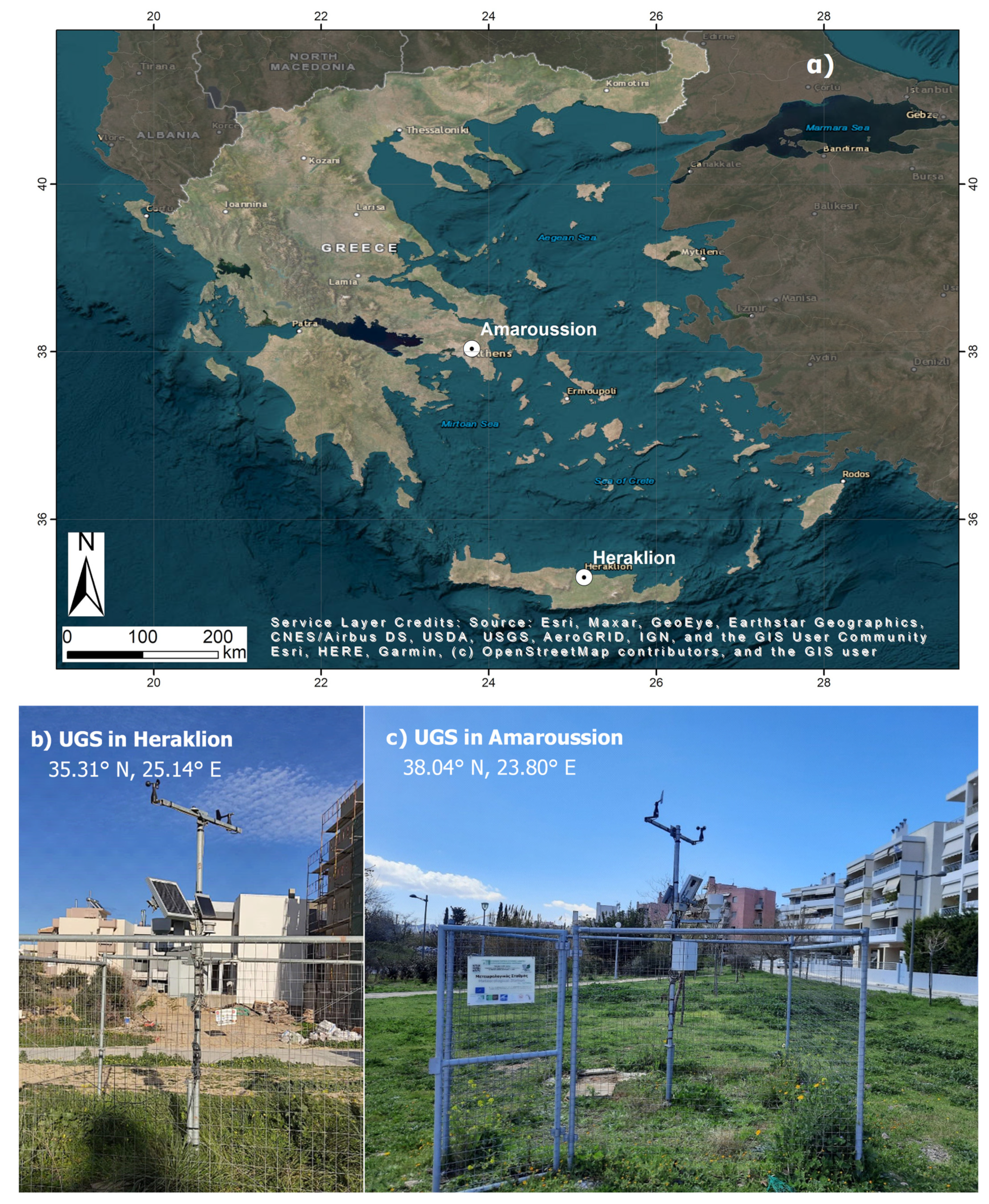
The present study was conducted in urban green areas in two cities in Greece: Amaroussion (central Greece) and Heraklion (South Greece-Crete island). The sites’ locations are presented in Figure 1.
The study site in Amaroussion (38.04°N, 23.80°E, alt.: 190 m a.s.l.) is in an urban green space with an area of 9.1 ha covered with a variety of plant species including grass, shrubs (e.g., Lavandula angustifolia Mill., Nerium oleander L., Rosmarinus officinalis L., Teucrium fruticans L.), herbaceous species (e.g., Calendula arvensis (Vaill.) L., Capsella bursa-pastoris (L.) Medik., Convolvulus arvensis L., Lactuca serriola L., Matricaria recutita L., Pallenis spinosa (L.) Cass., Plantago lanceolata L., Solanum elaeagnifolium Cav.), and generally deciduous broad-leaved tree species (e.g., Acer negundo L., Ailanthus altissima (Mill.) Swingle, Cercis siliquastrum L., Melia azedarach L., Morus alba L., Platanus orientalis L., Prunus cerasifera Ehrh., Tilia tomentosa Moench), in mixed patterns. The climate of the broader area is characterized as semi-arid [47,48,49], according to UNEP’s [50] aridity climate classification system based on Thornthwaite’s [51,52] water balance approach. A detailed description of the study site can be also found in Proutsos et al. [43] and in Solomou et al. [53].
The site in Heraklion (35.31°N, 25.14°E, alt.: 81 m a.s.l.) is located in the island of Crete in the southern part of Europe. It is also an urban green area covered to a lesser degree by vegetation. The vegetation in the site includes trees, shrubs and herbaceous plants. The trees are generally deciduous broad-leaved (e.g., Ficus carica L., F. elastica Roxb., Citrus reticulata L., C. limon L., Olea europaea L., Pinus brutia Tenore.) and randomly distributed in the site. The shrub-covered surfaces host a variety of species (e.g., Pittosporum tobira (Thunb.) W.T. Aiton, Nerium oleander L., Rosmarinus officinalis L.) in mixed patterns with herbaceous plants (e.g., Convolvulus arvensis L., Glebionis coronaria (L.) Spach, Malva sylvestris L., Medicago lupulina L., Oxalis pescaprae L.). The climate in the area is sub-humid [48,49] according UNEP’s [50] aridity classification system based on Thornthwaite’s [51,52] water balance approach, presenting also high decadal variability to warmer [54,55], more arid conditions [49,56] with more frequent droughts in the recent years compared to the past [55].
In the two sites, two micrometeorological stations were established for the constant monitoring of the aerial and soil environment. Both stations were equipped with sensors measuring temperature-relative humidity (EE08, E+E Elektronik Ges.m.b.H., Engerwitzdorf, Austria), wind speed and wind direction (Small Wind Transmitter, THIES CLIMA, Adolf Thies GmbH & Co. KG, Göttingen, Germany), precipitation (PROFESSIONAL, Pronamic ApS, Skjern, Denmark), global solar radiation at wavelengths 305–2800 nm (Pyranometer SP-Lite, ADCON Telemetry, Klosterneuburg, Austria, with a sensitivity change of 2% per year), and photosynthetically active radiation at 400–700 nm (QSO-S Quantum sensor, Apogee Instruments, Inc., Logan, Utah, USA, with ±5% accuracy). The measurements were conducted every 5 s, and the 10 min averages were recorded.
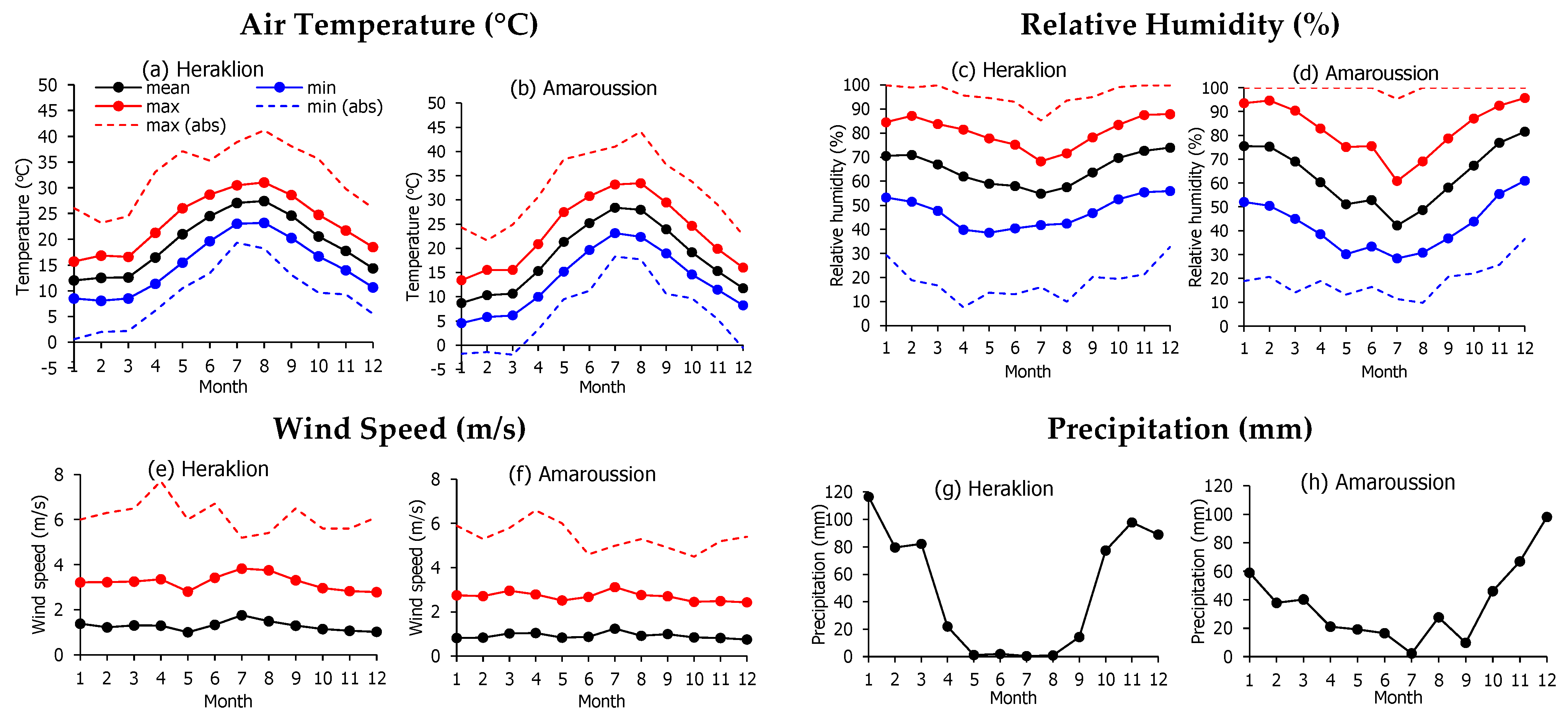
The available data cover the time period from 24 September 2019 to 31 December 2022 in Amaroussion and from 18 October 2019 to 31 December 2022 in Heraklion. During these periods, the monthly values of temperature, relative humidity, wind speed and precipitation in the two sites are presented in Figure 2. The acquired data patterns are rather expected for the climatic patterns of these areas.

2.2. PET Methods

The estimation of PET was performed by employing 112 empirical methods, which can be categorized into four distinct groups based on their required variables for their application:
  • 12 mass-transfer-based methods following the general form of PET = f (u, T, RH). These methods are based on the assumption that evapotranspiration is affected by the air movements considering also atmospheric dryness, which is expressed by the difference between air vapor pressure at saturation (es) and actual vapor pressure (ea). In all cases, the vapor pressure deficit effect is corrected by the addition of the aerodynamic term as a function of wind speed u. For the PET estimation, wind speed (u), air temperature (T) and relative humidity (RH) data are required. The analytical expressions of the 12 mass transfer empirical equations (Equations (1)–(12) used in this work are presented in Table 1.
  • 48 temperature-based methods following the general forms of PET = f (T), 34 methods (Equations (13)–(46)); PET = f (T, RH), 13 methods (Equations (47)–(59)); and PET = f (T, PR), 1 method (Equation (60)), presented in Table 2.
  • 40 radiation-based methods following the general forms of PET = f (Rs), 2 methods (Equations (61) and (62)); PET = f (Rs, T), 21 methods (Equations (63)–(83)); and PET = f (Rs, T, RH), 17 methods (Equations (84)–(100)), presented in Table 3.
  • 13 combination methods following the general forms of PET = f (Rs, u, T, RH), 12 methods, (Equations (101)–(111) and the benchmark method FAO56-PM [11]); and PET = f (Rs, u, T), 1 method (Equation (112)), presented in Table 4.
Table 1. Mass transfer-based methods. General form PET = f (u, T, RH).
Mass Transfer MethodsEquation PET = f (u, T, RH) *EquationRef.
Dalton 1802 PET = 3.648 + 0.7223 u e s e a (1)[57]
Fitzgerald 1886 PET = 4 + 1.99   u e s e a (2)[58]
Trabert 1896 PET = 3.075   u   e s e a (3)[59]
Meyer 1926 PET = 3.75 + 0.5026 u e s e a (4)[60]
Rohwer 1931 PET = 3.3 + 0.891 u e s e a (5)[61]
Penman 1948 PET = 2.625 + 1.3812   u   e s e a (6)[62]
Albrecht 1950 PET = 1.005 + 2.97   u   e s e a ,     for   u 1   m / s 4   e s e a ,     for   u > 1   m / s (7)[63,64]
Brock. and Wenner 1963 PET = 5.43   u 0.456   e s e a (8)[65]
WMO 1966 PET = 1.298 + 0.934   u   e s e a (9)[66]
Mahringer 1970 PET = 2.86   u   e s e a (10)[67]
Szász 1973 PET = 0.00536   T + 21 2   1 + RH 100 2 / 3 0.0519   u + 0.905 (11)[68]
Linacre 1992 PET = 0.015 + 0.0004   T + 0.000001   z 380   T + 0.006   z 84 φ 40 + 4 u   T T d (12)[69]
* where u is the wind speed at 2 m height in m s−1, T is the air temperature in °C, Td is the dew-point in °C, RH is the relative humidity in %, es and ea are the saturation and actual vapor pressures, respectively, in kPa, z is the altitude and φ is the geographical latitude in degrees.
Table 2. Temperature-based methods. General forms PET = f (T), PET = f (T, RH) and PET = f (T, PR).
Temperature-Based MethodsEquation PET = f (T) *EquationRef.
Thornthwaite 1948 PET = 16 10   T I a N 360 , I = 1 12 0.2   T 1.514 (13)[51,70]
Blaney and Criddle 1950 PET = 0.85   p   0.46   T + 8.13 ,       from   April   to   September 0.45   p   0.46   T + 8.13 ,       from   October   to   March (14)[71]
McCloud 1955 PET = 0.254   · 1.07 1.8   T (15)[72]
Hamon 1963 PET = 29.8   N   e s T   + 273.2 , for T > 0(16)[73,74]
Baier and Robertson 1965 PET = 0.157   T max + 0.158   T max T min + 0.109   R a 5.39 (17)[30]
Malmstrom 1969 PET = 40.9   e s N 360 (18)[73]
Siegert and Schrodter 1975 PET = 0.533 10   T 33.617 1.033 N 12 (19)[75]
Blaney and Criddle (Mid.Eu,. ver.) PET = 1.55 + 0.96   p   0.457   T + 8.128 (20)[19]
Smith and Stopp 1978 PET = 0.16   T (21)[76]
Hargreaves and Samani 1985 PET = 0.0023   T max T min 0.5   T + 17.8   R a (22)[77]
Kharrufa 1985 PET = 0.34   p   T 1.3 (23)[78]
Mintz and Walker 1993 PET = 0.17 N 12 T (24)[79]
Camargo et al. 1999 PET = 16 10   T ef I a N 360 , I = 1 12 0.2   T ef 1.514 , T ef = 0.36 3 T max T min (25)[80]
Samani 2000 PET = 0.0135   KT   R a   T max T min 0.5   T + 17.8
KT = 0.00185   T max T min 2 0.0433   T max T min + 0.4023
(26)[77,81,82]
Xu and Singh 2001 (1) PET = 20 10   T I a N 360 , I = 1 12 0.2   T 1.514 (27)[83]
Xu and Singh 2001 (2) PET = 20.5 10   T I a N 360 , I = 1 12 0.2   T 1.514 (28)[83]
Xu and Singh 2001 (3) PET = 0.37   p   T 1.3 (29)[83]
Xu and Singh 2001 (4) PET = 0.0028   T max T min 0.5   T + 17.8   R a (30)[83]
Droogers and Allen 2002 (1) PET = 0.0030   T max T min 0.4   T + 20   R a (31)[84]
Droogers and Allen 2002 (2) PET = 0.0025   T max T min 0.5   T + 16.8   R a (32)[84]
Pereira and Pruitt 2004 PET = 16 10   T ef I a N 360 , I = 1 12 0.2   T ef 1.514   T ef = 0.345 3 T max T min N 24 N for T T ef T max (33)[70]
Trajcovic 2005 (1) PET = 0.88 16 10   T I a N 360 + 0.565 , I = 1 12 0.2   T 1.514 (34)[85]
Trajcovic 2005 (2) PET = 0.817   0.0023   T max T min 0.5   T + 17.8   R a + 0.320 (35)[85]
Oudin 2005 PET = R a T + 5 100 , for T + 5 > 0 (36)[86]
Castañeda and Rao 2005 (1) PET = 0.9   p   0.46   T + 8.13 ,       from   April   to   September 0.6   p   0.46   T + 8.13 ,       from   October   to   March (37)[87]
Trajkovic 2007 PET = 0.0023   T max T min 0.424   T + 17.8   R a (38)[31]
Tabari and Talaee 2011 (1) PET = 0.0031   T max T min 0.5   T + 17.8   R a (39)[88]
Tabari and Talaee 2011 (2) PET = 0.0028   T max T min 0.5   T + 17.8   R a (40)[88]
Ravazzani et al. 2012 PET = 0.817 + 0.00022 z   0.0023 R a   T + 17.8 T max T min 0.5 (41)[89]
Berti et al. 2014 PET = 0.00193   R a   T + 17.8 T max T min 0.517 (42)[90]
Heydari and Heydari 2014 PET = 0.0023   T max T min 0.611   T + 9.519   R a (43)[91]
Dorji et al. 2016 PET = 0.002   T max T min 0.296   T + 33.9   R a (44)[92]
Lobit et al. 2018 PET = 0.1555   R a 0.00428   T + 0.09967   T max T min 0.5 (45)[93]
Althoff et al. 2019 PET = 0.0135 · 0.166   R a   T max T min 0.5   T + 15.3 (46)[94]
Equation PET = f (T, RH) *
Romanenko 1961 PET = 0.0018   25 + T 2   100 RH N 360 (47)[95]
Papadakis 1965 PET = 2.5   e ma e d (48)[96]
Schendel 1967 PET = 16   T RH (49)[29]
Antal 1968 PET = 0.736   e s e a 0.7   1 + T 273 4.8   (50)[97,98]
Linacre 1977 PET = 500 T + 0.006 z 100 φ + 15 T T d / 80 + T (51)[99]
Naumann 1987 PET = 0.18   N   e s 14 e a 14 (52)[100]
Xu and Singh 2001 (5) PET = 0.0020   25 + T 2   100 RH N 360 (53)[83]
Xu and Singh 2001 (6) PET = 488 T + 0.006 z 100 φ + 15 T T d / 80 + T (54)[83]
Xu and Singh 2001 (7) PET = 615 T + 0.006 z 100 φ + 15 T T d / 80 + T (55)[83]
Ahooghalaandari et al. 2016 (1) PET = 0.252   R a + 0.221   T 1 RH 100   (56)[101]
Ahooghalaandari et al. 2016 (2) PET = 0.29   R a + 0.15   T max 1 RH 100 (57)[101]
Ahooghalaandari et al. 2016 (3) PET = 0.369   R a + 0.139   T max 1 RH 100 1.95 (58)[101]
Ahooghalaandari et al. 2016 (4) PET = 0.34   R a + 0.182   T 1 RH 100 1.55 (59)[101]
Equation PET = f (T, PR) *
Droogers and Allen 2002 (3) PET = 0.0013   T max T min 0.0123 PR 0.76   T + 17   R a (60)[84]
* where a = 6.75 × 10⁻⁷ I3 − 7.71 × 10⁻⁵ I2 +1.7912 × 10⁻² I + 0.49239 (Equations (13), (25), (27), (28), (33) and (34)), p represents the daily percentage (%) of annual daytime hours for each day of the year, N represents the maximum sunshine daily hours, T, Tmax and Tmin are the daily mean, maximum and minimum air temperatures in °C, Td is the dewpoint in °C, RH is the relative humidity in %, φ is the latitude in degrees, z is the altitude in m, PR is the monthly precipitation in mm, Ra is the extraterrestrial radiation in mm day−1 in all equations except those from Baier and Robertson 1965 (Equation (17)) and Lobit et al. 2018 (Equation (45)), where Ra is in MJ m−2 d−1, es and ea are the saturation and actual vapor pressures in kPa in all equations except those from Antal 1968 (Equation (50)), where they are in hPa, ema is the saturation vapor pressure at daily maximum temperature in kPa and es14 and ea14 are the es and ea values in kpa at 14 h local time.
Table 3. Radiation-based methods PET = f (Rs) and PET = f (Rs, T, RH).
Radiation-Based MethodsEquation PET = f (Rs) *EquationRef.
Christiansen 1968 PET = 0.385   R s λ   (61)[102]
Abtew 1996 (1) PET = 0.52 R s λ (62)[103]
Equation PET= f (Rs, T) *
Makkink 1957 PET = 0.61   Δ Δ + γ   R s λ 0.12 (63)[104]
Steph. and Stewart 1963 PET = 0.0082   9 5   T + 32 0.19   23.9   R s 1500 25.4 (64)[105]
Jensen and Haise 1963 PET = R s λ 0.025   T + 0.08 (65)[106]
Stephens 1965 PET = 0.0158   T 0.09   R s (66)[107,108]
McGuin. and Bord. 1972 PET = 0.0059685   T + 0.02927624   R s (67)[109]
Ritchie 1972 PET = a 1   0.00387   R s   0.6   T max + 0.4   T min + 29 ,
a 1 = 1.1 ,   for   5   ° C < T max < 35   ° C 1.1 + 0.05 T max 35 ,   for   T max > 35   ° C 0.1 + e 0.18 T max + 20 ,   for   5 < T max < 5   ° C
(68)[110,111]
Caprio 1974 PET = 6.1   10 3   R s   1.8   T + 1 (69)[112]
Hargreaves 1975 PET = 0.0135   R s λ T + 17.8 (70)[113]
Hansen 1984 PET = 0.7 Δ Δ + γ   R s λ (71)[114]
de Bruin 1987 PET = 0.65 Δ Δ +   γ   R s λ (72)[115,116,117]
Wendl. 1991–1995 PET = 100   R s + 93 K T + 22 150 T + 123 (73)[118,119]
Abtew 1996 (2) PET = 0.012   23.89   R s + 50   T max T max + 15 (74)[103]
Abtew 1996 (3) PET = 1 56 T max   R s λ (75)[103]
Irmak et al. 2003 (1) PET = 0.149   R s + 0.079   T 0.611 (76)[120]
Irmak et al. 2003 (2) PET = 0.286   R s + 0.134   T 2.959 (77)[120]
Irmak et al. 2003 (3) PET = 0.264   R s 0.052 T max + 0.233   T min 1.110 (78)[120,121]
Castañeda and Rao 2005 (2) PET = 0.70   Δ Δ + γ   R s λ 0.12 (79)[87]
Valiantzas 2013 (1) PET = 0.0393   R s   T + 9.5 0.19   R s 0.6   φ 0.15 + 0.0061   T + 20   1.12   T T min 2 0.7 (80)[122,123]
Tabari et al. 2013 (1) PET = 0.642 + 0.174   R s + 0.0353   T (81)[124]
Tabari et al. 2013 (2) PET = 0.478 + 0.156   R s 0.0112   T max + 0.0733   T min (82)[124]
Ahooghal. et al. 2017 (1) PET = 0.79 · 0.0393   R s   T + 9.5 0.94 · 0.19   R s 0.6   φ 0.15 + 2.21 · 0.0061   T + 20   1.12   T T min 2 0.7 (83)[125]
Equation PET = f (Rs, T, RH) *
Turc 1961 PET = 0.013   23.9   R s + 50 T T + 15   ,   for   RH > 50 0.013   23.9   R s + 50 T T + 15   1 + 50 RH 70 ,   for   RH 50 (84)[126]
Priestley and Taylor 1972 PET = 1.26   Δ Δ + γ   R n G λ (85)[127]
Abtew 1996 (4) PET = 1.18   Δ Δ + γ   R n G λ (86)[103,128]
Xu and Singh 2000 PET = 0.98   Δ Δ + γ   R n G λ 0.94 (87)[129]
Irmak et al. 2003 (4) PET = 0.289   R n + 0.023   T + 0.489 (88)[120]
Irmak et al. 2003 (5) PET = 0.435   R n + 0.095   T 1.149 (89)[120]
Irmak et al. 2003 (6) PET = 0.432   R n + 0.043   T max + 0.055   T min 1.077 (90)[120,121]
Bereng. and Gavil. 2005 PET = 1.65   Δ Δ + γ   R n G λ (91)[130]
Copais PET = m 1 + m 2   C 2 + m 3   C 1 + m 4   C 1   C 2 ,
where m1 = 0.057, m2 = 0.277, m3 = 0.643, m4 = 0.0124
C 1 = 0.6416 0.00784   RH + 0.372   R s 0.00264   R s   RH
C 2 = 0.0033 + 0.00812   T + 0.101   R s + 0.00584   R s   T
(92)[131]
Valiantzas 2006 (1) PET = 0.038   R s   T + 9.5 2.4 R s R a 2 + 0.075   T + 20 1 RH 100 (93)[132]
Tabari and Talaee 2011 (3) PET = 2.14   Δ Δ + γ   R n G λ (94)[88]
Tabari and Talaee 2011 (4) PET = 1.82   Δ Δ + γ   R n G λ (95)[88]
Valiantzas 2013 (2) PET = 0.0393   R s   T + 9.5 0.19   R s 0.6   φ 0.15 + 0.078   T + 20 1 RH 100 (96)[122,123]
Valiantzas 2013 (3) PET = 0.0393   R s   T + 9.5 2.4 R s R a 2 0.024   T + 20 1 RH 100 + 0.1   W aero   T + 20 1 RH 100
W aero = 0.78 ,     for   RH > 65 % 1.067 ,     for   RH 65 %
(97)[133]
Milly and Dunne 2016 PET = 0.8   R n G λ (98)[134]
Ahooghal. et al. 2017 (2) PET = 0.79 · 0.0393   R s   T + 9.5 1.15 · 2.4 R s R a 2 3.23 · 0.024   T + 20 1 RH 100 + 0.32 · 0.1   W aero   T + 20 1 RH 100 ,
W aero = 0.78 ,     for   RH > 65 % 1.067 ,     for   RH 65 %
(99)[125]
Ahooghal. et al. 2017 (3) PET = 0.79 · 0.0393   R s   T + 9.5 0.94 · 0.19   R s 0.6   φ 0.15 + 1.37 · 0.078   T + 20 1 RH 100 (100)[125]
* where T, Tmax and Tmin represent the average, maximum and minimum daily air temperatures in °C, RH is the relative humidity in %, φ is the latitude in radians, Rs, Rn and Ra are the global solar, the net and the extraterrestrial radiation fluxes, respectively, in MJ m−2 day−1, G is the soil heat flux in MJ m−2 day−1 (G = 0), Δ is the slope of the vapor pressure curve (kPa °C−1), γ is the psychrometric constant (kPa °C−1) and λ = 2.501–0.002361 Τ, in MJ kg−1.
Table 4. Combination methods.
Combination MethodsEquation PET = f (Rs, u, T, RH) *EquationRef.
FAO56-PM PET = 0.408   Δ   R n G + γ   900 T + 273   u   e s e a Δ + γ 1 + 0.34   u Benchmark method[11]
Penman 1963 PET = Δ Δ + γ   R n G + 6.43 γ Δ + γ   1 + 0.537   u e s e a 1 λ (101)[135]
Kimberly Penman 1972 PET = Δ Δ + γ   R n G + 6.43 γ Δ + γ   0.75 + 0.993   u e s e a 1 λ (102)[24]
mod. Makkink (Door. and Pr. 1977) PET = b   Δ Δ + γ   R s λ 0.3 , b = 1.165 + 0.043 ub − 0.00575 RH (103)[19]
FAO24 Penman PET = Δ Δ + γ   R n G + 6.43 γ Δ + γ   1 + 0.862   u e s e a 1 λ (104)[19]
FAO24 Radiation PET = b Δ Δ + γ R s 0.3
b = 1.066 − 0.0013 RH + 0.045 u − 0.0002 RH u − 0.0000315 RH2 − 0.0011 u2
(105)[19,136]
Jensen et al. 1990 PET = Δ Δ + γ   R n G + 6.43 γ Δ + γ   a w + b w   u e s e a 1 λ .
a w = 0.4 + 1.4   e J 173 58 2 , b w = 0.605 + 0.345   e J 243 80 2
(106)[21,22]
Linacre 1993 PET = 0.015 + 0.00042   T + 0.000001   z   9.26   Rs 40 + 2.5 1 0.000087 z   u   T T d (107)[137]
Wright 1996 PET = Δ Δ + γ   R n G + 6.43 γ Δ + γ   a w + b w   u e s e a 1 λ
a w = 0.3 + 0.58   e J 170 45 2 , b w = 0.32 + 0.54   e J 228 67 2
(108)[23]
Valiantzas 2006 (2) PET = 0.038   R s   T + 9.5 2.4 R s R a 2 + 0.048   T + 20 1 RH 100   0.5 + 0.536 u + 0.00012   z (109)[132]
Valiantzas 2013 (4) PET = 0.0393   R s   T + 9.5 0.19   R s 0.6   φ 0.15 + 0.048   T + 20 1 RH 100   u 0.7 (110)[122,123]
Valiantzas 2013 (5) PET = 0.0393   R s   T + 9.5 2.4 R s R a 2 0.024   T + 20 1 RH 100 + 0.066   W aero   T + 20 1 RH 100   u 0.6 , W aero = 0.78 ,     for   RH > 65 % 1.067 ,     for   RH 65 % (111)[133]
PET = f (Rs, u, T) *
Valiantzas 2013 (6) PET = 0.0393   R s   T + 9.5 0.19   R s 0.6   φ 0.15 + 0.0037   T + 20   1.12   T T min 2 0.7 u 0.7 (112)[122,123]
* where T and Tmin are the average and minimum daily air temperatures in °C, Td is the dewpoint in °C, RH is the relative humidity in %, φ is the latitude in radians, z is the altitude in m, Rs, Rn and Ra are the global solar, the net and the extraterrestrial radiation fluxes in MJ m−2 day−1, G is the soil heat flux in MJ m−2 day−1 (G = 0), Δ is slope of the vapor pressure curve (kPa °C−1), γ is the psychrometric constant (kPa °C−1), J is the day of the year, λ= 2.501 − 0.002361 Τ, in MJ kg−1, es and ea are the saturation and actual vapor pressures in kPa, u is the windspeed at height 2m in m/s and ub is the windspeed in Beaufort.
The equations of all models used in this work are presented for each group below. Details for the estimation of the parameters used in the equations can be found in Allen et al. [11] and Proutsos et al. [138,139]. The PET estimates with negative values were excluded for the analysis.

2.3. Statistical Indices and Ranking

To compare the estimations of PET by the different models against the estimates by FAO56-PM, the commonly used coefficients of the linear regression y = ax + b were employed: slope a, intercept b and coefficient of determination R2. Four additional statistical measures recommended by Fox [140] were applied: the mean bias error (MBE) to assess the bias, the variance of the differences distribution s d 2 to evaluate the variability of the differences between the PET values around the MBE, the mean absolute error (MAE) and the root mean square error (RMSE) to express the average difference. The index of agreement (d) was also used to make the cross-comparison between the models [141,142,143]. The analytic equations for the estimation of the indices are presented in Appendix A (Equations (A1)–(A5)).
To rank the methods, the above indices were used, and through a standardization procedure proposed by Aschonitis et al. [144] and also described in Rahimikhoob et al. [145], the standardized ranking performance index (sRPI) was estimated by the equations presented in Appendix A (Equations (A6)–(A9)).

3. Results

The micrometeorological stations of this study were installed above grass-covered irrigated surfaces inside the urban green spaces. Such surface characteristics allow the accurate estimation of PET by the application of the Penman–Monteith method considering that the measured meteorological parameters are highly affected by the substrate above which the measurements are taken [8].
The PET estimates with the FAO56-PM method for the two cities present higher values for the southern site of Heraklion with an annual average of 3.37 ± 1.92 mm d−1, which is slightly higher compared to the respective values of Amaroussion (3.10 ± 1.92 mm d−1). Both sites present high seasonal variability with ET values ranging from 1.44 ± 0.49 mm d−1 in winter to 5.87 ± 0.77 mm d−1 in summer in Heraklion and from 1.05 ± 0.41 mm d−1 in winter to 5.48 ± 1.00 mm d−1 in summer in Amaroussion. The day-to-day and monthly values are even more variable, as depicted in Figure 3.
The daily values of Figure 3 were used as the basis for comparing PET with the respective estimates by the application of other methods. The results per method category follow.

3.1. Mass Transfer-Based Methods

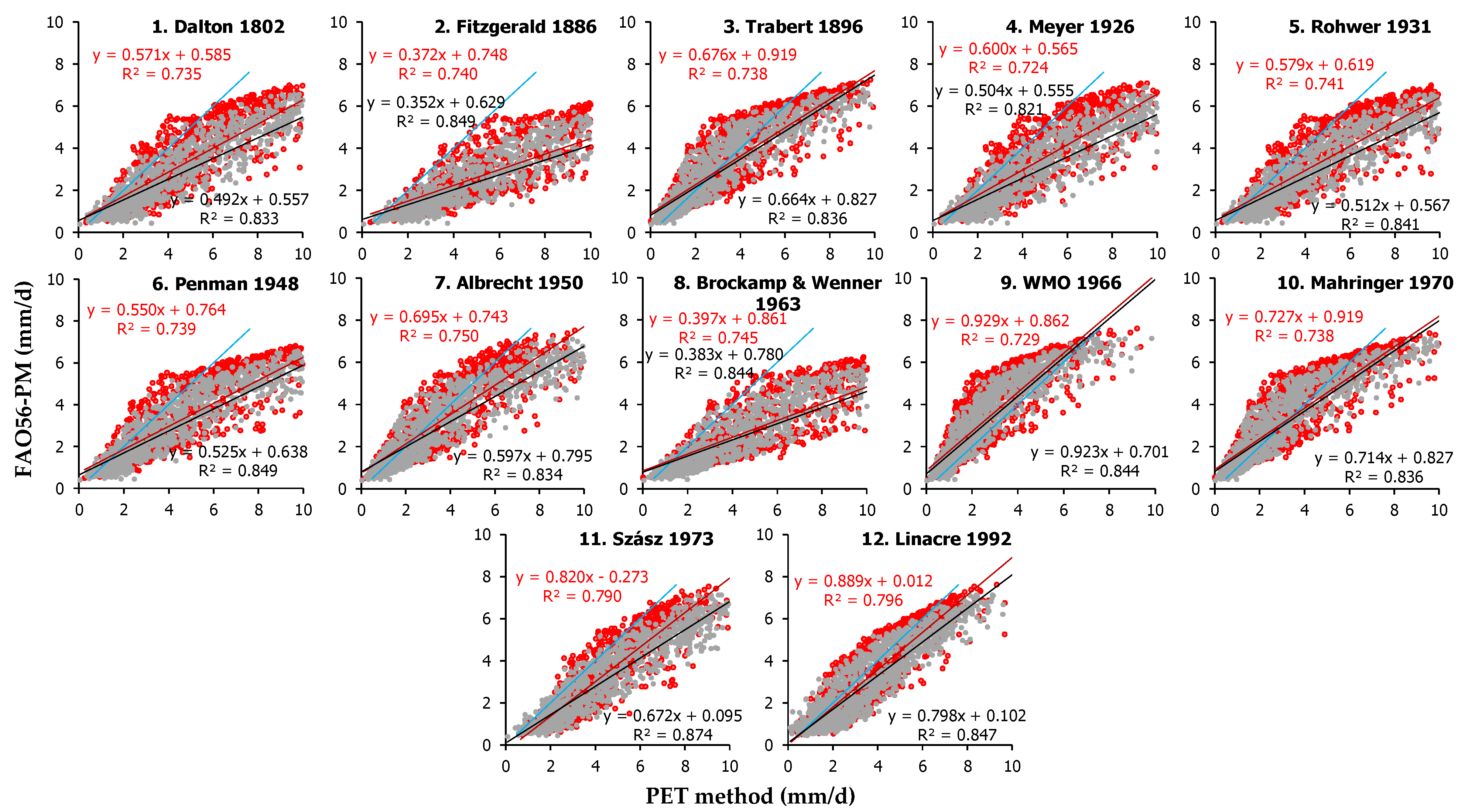
The comparative presentation of the PET estimates produced by the application of the 12 mass transfer methods (Equations (1)–(12)) against the PET values by the FAO56-PM method for the two urban green areas are presented in Figure A1, Appendix B, along with the regression line statistics. The values dispersion confirms the higher PET in Heraklion compared to Amaroussion. The combined assessment of Figure A1 (Appendix B) and Table A1 (Appendix C) indicates that in general, Mahringer 1970 (Equation (10)) followed by Trabert 1886 (Equation (3)) and Linacre 1992 (Equation (12)) are the best performing mass transfer-based methods in Heraklion, ranking 46th, 47th and 52nd among all 112 examined models with sRPI scores of 0.827, 0.825 and 0.813, respectively (Table 5), whereas Fitzerald 1986 (Equation (2)) and Brockamp and Wenner 1963 (Equation (8)) are the worst (112th with sRPI = 0.177 and 111th with sRPI = 0.292, respectively, at the overall ranking). Mahringer 1970 (Equation (10)) produced the minimum MBE (−0.029 mm d−1) and the best slope a value (1.015) compared to all other mass transfer methods, whereas its mean value (3.234 ± 2.264 mm d−1) is quite close to FAO56-PM (3.266 ± 1.910 mm d−1) and only underestimated by −0.98%. Trabert 1886 (Equation (3)) had the best d index (0.974) and Linacre 1992 (Equation (12)) had the smallest RMSE (0.977 mm d−1), smallest MAE (0.801), smallest sd2 (0.789 mm d−1), and best R2 (0.796) among all mass transfer-based method in Heraklion.
In the green space of Amaroussion, however, WMO 1966 (Equation (9)), Linacre 1992 (Equation (12)) and Mahringer 1970 (Equation (10)) were the best-performing mass transfer-based methods (Table 5), ranking 40th, 44th and 50th, with sRPI scores of 0.853, 0.831 and 0.826, respectively. The worst methods were also Fitzerald 1986 (Equation (2)) and Brockamp and Wenner 1963 (Equation (8)), as in Heraklion, which were ranked 112th and 111th among all methods with sRPI values of 0.189 and 0.300, respectively. WMO 1966 (Equation (9)) produced the minimum MAE (0.693 mm d−1), RMSE (0.923 mm d−1) and the best sd2 (0.592 mm d−1) and d (0.982) values, but its average PET estimate (2.465 ± 1.905 mm d−1) was −17% smaller compared to FAO56-PM (2.969 ± 1.904 mm d−1). Linacre 1992 (Equation (12)) had the best slope a value (1.062).
The ranking scores for both sites (derived as averages of the sRPI) suggest that Mahgringer 1970 (Equation (10)) had the best performance among the mass transfer methods, followed by WMO 1966 (Equation (9)) and Linacre 1992 (Equation (12)), which ranked 45th, 47th and 49th among the 112 examined models with sRPI values of 0.827, 0.826 and 0.822, respectively. The correlations of the five best-performing models of this category are presented in Figure 4.

3.2. Temperature-Based Methods

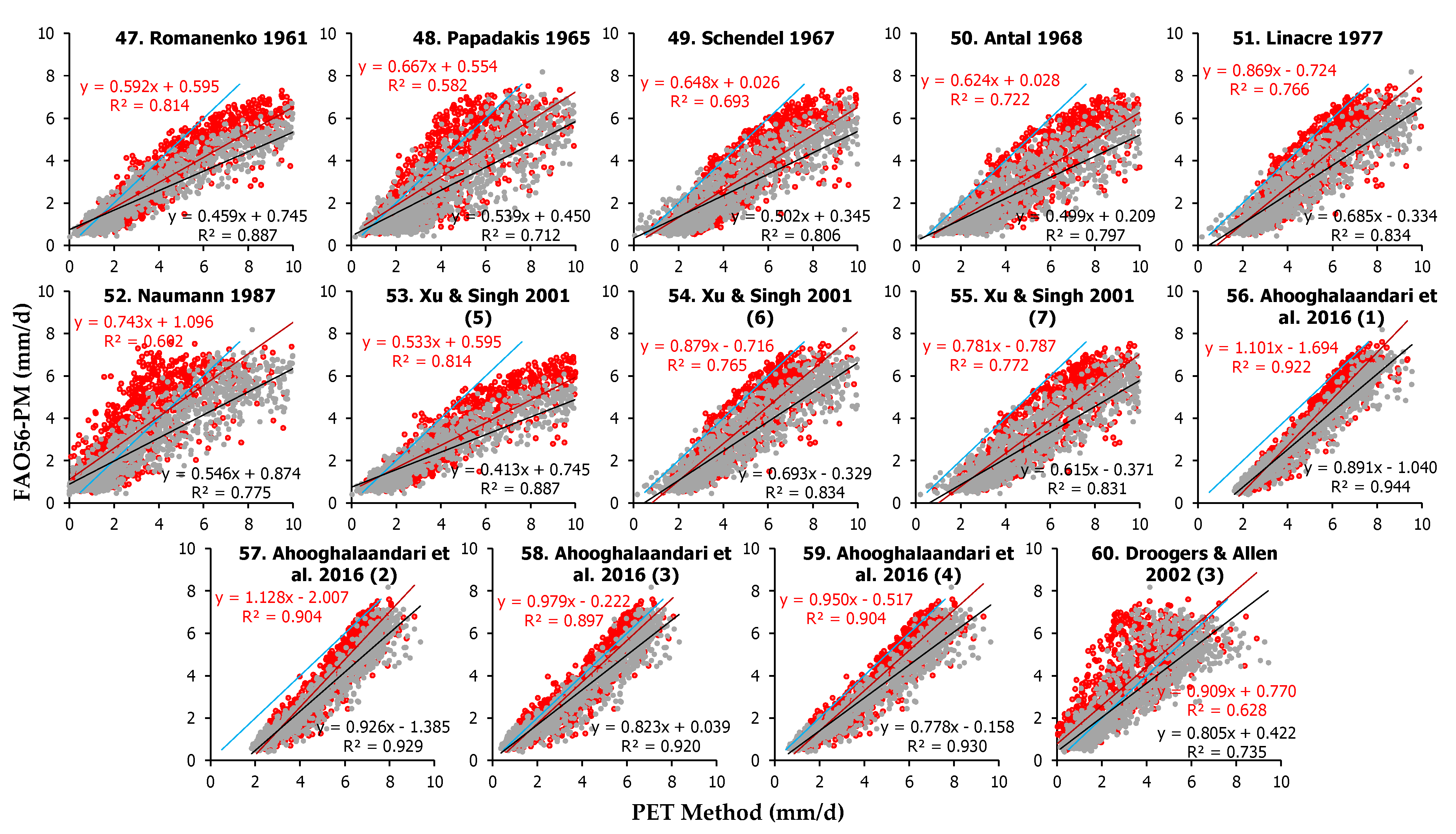
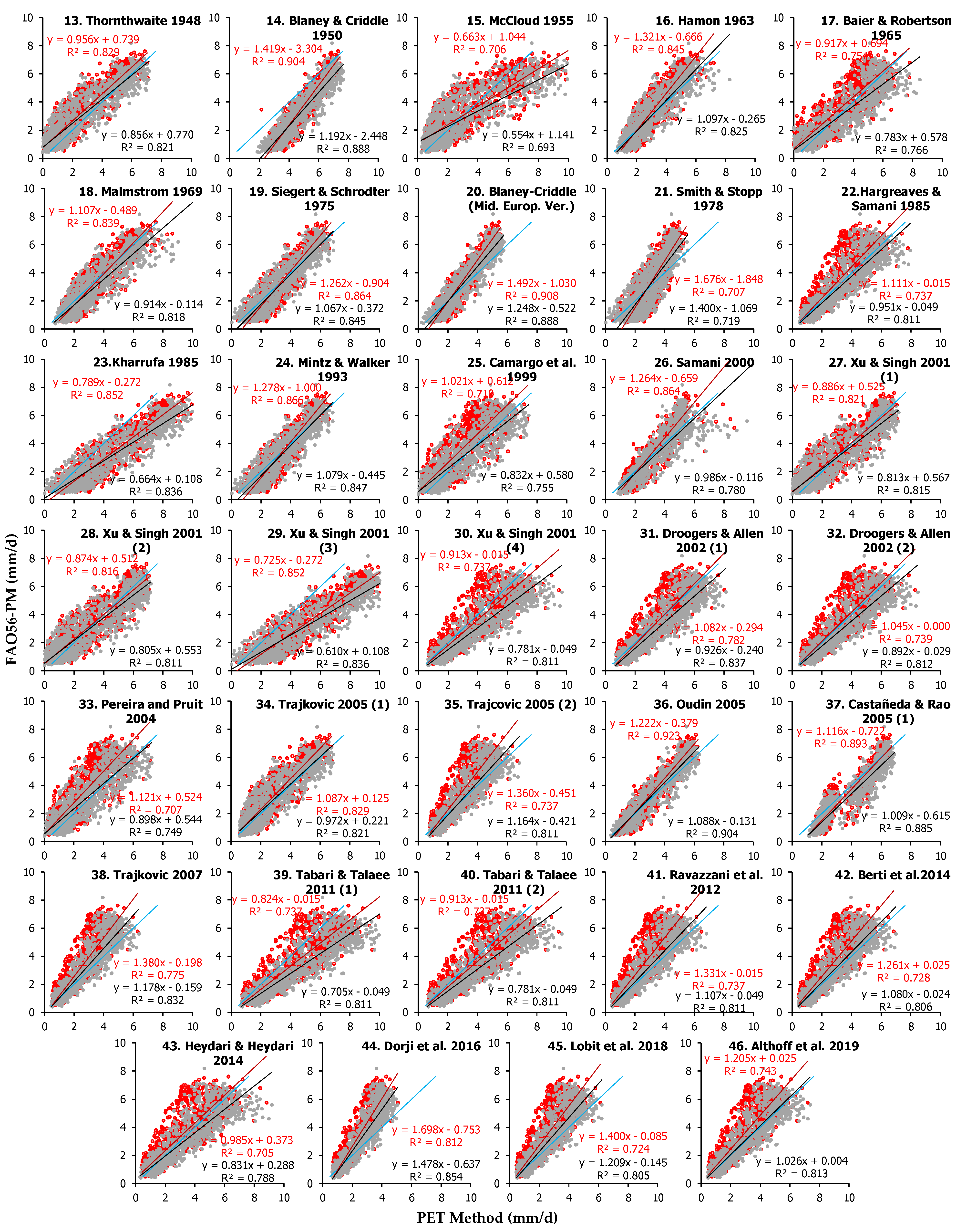
The PET estimates by the application of 48 temperature-based empirical models (Equations (13)–(60)) are presented against the respective daily values by FAO56-PM for the two sites in Figure A2 and Figure A3 (Appendix B). The general patterns indicate generally higher estimates of the method of this category in Heraklion compared to the site in Amaroussion. The statistics from the comparisons for all methods in both sites are presented in Table A2 (Appendix C).
In Heraklion, Ahooghalaandari et al. 2016 (3) (Equation (58)) was the best temperature-based method, ranking 27th among all examined models with sRPI = 0.889, followed by Xu and Singh 2001 (2) (Equation (28)) and Xu and Singh 2001 (1) (Equation (27)), which ranked 34th and 37th, with sRPI values of 0.876 and 0.869, respectively. Ahooghalaandari et al. 2016 (3) (Equation (58)) had the minimum MAE (0.562 mm d−1) and the best d (0.966) values, and they produced an average PET (3.609 ± 2.451 mm d−1) +10% higher compared to FAO56-PM. The worst temperature-based methods for the site were by Antal 1968 (Equation (50)) and Smith and Stopp 1978 (Equation (21)), which ranked 109th and 108th among the 112 models.
Ahooghalaandari et al. 2016 (3) (Equation (58)) was also the best method for the site of Amaroussion, ranking 26th among the 112 tested models with a similar sRPI (0.887), which was followed by Oudin 2005 (Equation (36)) and Xu and Singh 2001 (2) (Equation (28)) ranking 27th (sRPI = 0.885) and 36th (sRPI = 0.861), respectively. The worst performing were the methods of Xu and Singh 2001 (5) (Equation (53)) and Antal 1968 (Equation (50)), which were ranked 110th and 109th with sRPI scores 0.407 and 0.489, respectively. The application of Ahooghalaandari et al. 2016 (3) (Equation (58)) produced an average PET of 3.607 ± 2.720 mm d−1, which was +21% higher compared to FAO56-PM.
The statistical indices and the ranking (among the 112 examined models) for the five best-performing temperature-based methods for each site are shown in Table 6.
For both sites, Ahooghalaandari et al. 2016 (3) (Equation (58)), Oudin 2005 (Equation (36)) and Xu and Singh 2001 (2) (Equation (28)) are ranked higher among the temperature-based PET methods (27th, 31st and 35th, respectively, at the overall ranking) with sRPI scores of 0.888, 0.877 and 0.869, respectively. It is worth noting that all 48 temperature-based methods received sRPI scores ranging from 0.487 to 0.888, and 15 of them had sRPI values greater than 0.800, whereas 4 out of the 12 mass transfer-based methods had sRPIs greater than 0.800. The correlations of the daily value estimated by the five best-performing methods of this category against the FAO56-PM method are presented for both sites in Figure 5.

3.3. Radiation-Based Methods

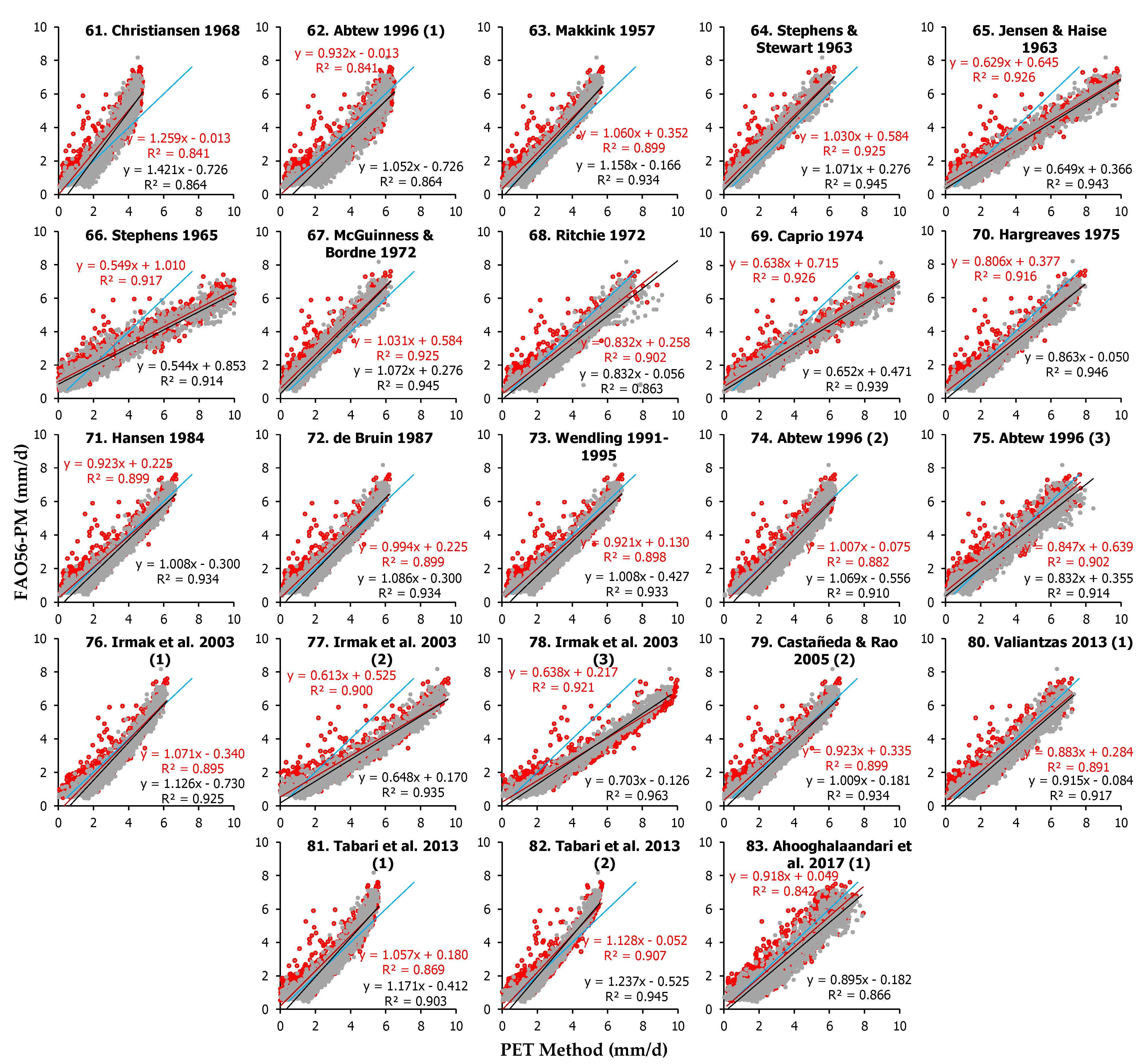
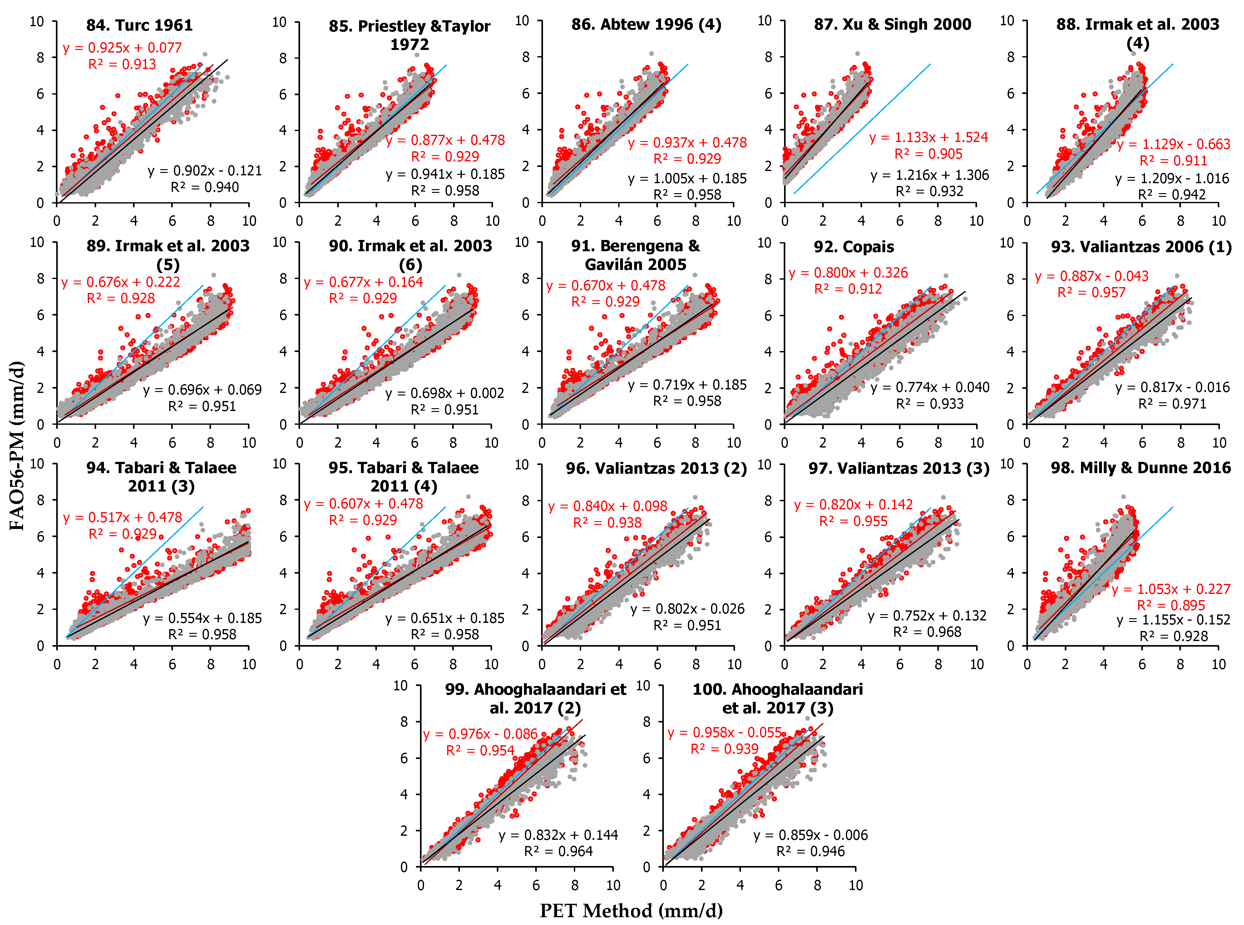
The 40 radiation-based methods (Equations (61)–(100)) examined in the two study sites produced daily estimates presented in conjunction with the FAO56-PM estimates in Figure A4 and Figure A5 (Appendix B). The comparison between the values produced the statistics presented in Table A3 (Appendix C). The statistical indices for the five best-performing radiation-based methods in each site are presented in Table 7.
In Heraklion, the best-performing radiation-based methods were Ahooghalaandari et al. 2017 (2) (Equations (99)) followed by Castañeda and Rao 2005 (2) (Equation (79)) and Priestley and Taylor 1972 (Equation (85)), which were ranked 4th, 8th and 9th among all 112 models, with sRPI scores of 0.955, 0.943 and 0.941, and mean PET estimates +7.7%, −0.7% and −0.5% different compared to FAO56-PM, respectively. Ahooghalaandari et al. 2017 (2) (Equation (99)) presented minimum RMSE (0.534 mm d−1), MAE (0.416 mm d−1) and sd2 (0.178), whereas Castañeda and Rao 2005 (2) (Equation (79)) had the minimum offset b (−0.007 mm d−1) and Priestley and Taylor 1972 (Equation (85)) had the minimum MBE (−0.014 mm d−1) and the best d (0.986) among the radiation-based models. The worst methods of this category in Heraklion were Tabari and Talaee 2011 (3) (Equation (94)) ranking 110th sRPI = 0.495 and Xu and Singh 2000 (Equation (87)) ranking 103rd with sRPI = 0.603, producing PET means −30.7% and +67.6% different compared to FAO56-PM. In general, however, the radiation methods in Heraklion had a good performance in most cases, since the produced PET means were less than 10% different from FAO56-PM in 19 out of the 40 methods.
In Amaroussion, Priestley and Taylor 1972 (Equation (85)) was ranked first among the radiation-based methods (2nd among all 112 models, with sPRI = 0.972), followed by Abtew 1996 (4) (Equation (86)) and Ahooghalaandari et al. 2017 (2) (Equation (99)), which were ranked 6th (sPRI = 0.956) and 9th (sPRI = 0.933) among all examined models. These methods produced mean PET values +2.00%, −4.3% and +17% different compared to FAO56-PM, respectively. Priestley and Taylor 1972 (Equation (85)) showed the best MBE (−0.014 mm d−1), RMSE (0.486 mm d−1) and d (0.992) values, whereas Abtew 1996 (4) (Equation (86)) had the best MAE (0.374 mm d−1) and sd2 (0.229 mm d−1) and Ahooghalaandari et al. 2017 (2) (Equation (99)) presented the minimum offset b (−0.045 mm d−1) among all radiation-based methods. The worst models in Amaroussion were Tabari and Talaee 2011 (3) (Equation (94)) and Xu and Singh 2000 (Equation (87)), ranking 103rd and 99th, respectively, among all examined 112 methods, with sRPI values of 0.591 and 0.621. These methods’ mean PET values were +71.7% and −28.7% different compared to FAO56-PM. The overall performance of radiation-based methods in Amaroussion can be considered satisfactory, considering that 28 out of the 40 equations presented sRPI values higher than 0.800, whereas 15 of them had sRPI > 0.900.
The ranking derived from the statistics of both sites suggests that Priestley and Taylor 1972 (Equation (85)) ranking 5th with sRPI = 0.957, Abtew 1996 (4) (Equation (86)) ranking 7th with sRPI = 0.946 and Ahooghalaandari et al. 2017 (2) (Equation (99)) ranking 9th with sRPI = 0.944 between all 112 models were the best radiation-based methods, whereas Tabari and Talaee 2011 (3) (Equation (94)) ranking 107th and Xu and Singh 2000 (Equation (87)) ranking 102nd were the two worst methods with average sPRI values from both sites 0.543 and 0.612, respectively. The best five performing methods for both sites (according to the average sRPI scores) are depicted in Figure 6.

3.4. Combination Methods

The PET estimates from the 12 combination methods (Equations (101)–(112)) assessed in this study are depicted against the PET daily values in Figure A6 (Appendix B), whereas the statistical indices values used for the ranking of the methods are presented in Table A4 (Appendix C). The graphs and the statistical results suggest that this category of models produces good PET estimates compared to all other categories.
The statistics for five best-performing methods of this PET model category are presented for both sites in Table 8. The assessment of all combination methods statistics, presented also in Table A4 (Appendix C), indicates that Wright 1996 (Equation (108)) is the best-performing model in Heraklion, followed by Valiantzas 2006 (2) (Equation (109)) and Jensen et al. 1990 (Equation (106)). Wright 1996 (Equation (108)) is ranked 1st among all examined 112 models and had the best sRPI (0.987), whereas it produced an average PET that was only −0.8% lower compared to FAO56-PM. This method presented the minimum RMSE (0.446 mm d−1) and MAE (0.315 mm d−1) and also the best slope a (1.005) and d (0.989) values. Valiantzas 2006 (2) (Equation (109)) and Jensen et al. 1990 (Equation (106)) methods were ranked 2nd and 3rd, respectively, among all 112 examined models and had also high sRPI values (0.970 and 0.963). However, the produced mean PET values were about +11% higher compared to FAO56-PM. However, Valiantzas 2006 (2) (Equation (109)) presented the minimum offset b (−0.008 mm d−1) and sd2 (0.078 mm d−1) in Heraklion not only among the combination but among all 112 methods. The worst-performing methods for the site were FAO24 Radiation (Equation (105)) followed by the modified Makkink by Doorenbos and Pruitt 1977 (Equation (103)), which were ranked 58th and 53rd with sRPI values of 0.792 and 0.813, respectively. The mean PET values of these methods were +25.3% and +20.4% higher compared to FAO56-PM.
In Amaroussion, Wright 1996 (Equation (108)) was the best-performing model ranked 1st with sRPI = 0.992 followed by Jensen et al. 1990 (Equation (106)), Valiantzas 2006 (2) (Equation (109)), and Valiantzas 2013 (6) (Equation (112)), which were ranked 3rd, 4th and 5th with similar sRPI values (0.963, 0.962 and 0.962). Wright 1996 (Equation (108)) showed the best slope a (0.984) and d (0.991) and the minimum RMSE (0.393 mm d−1), MAE (0.264 mm d−1) and sd2 (0.159 mm d−1) values, producing a mean PET estimate +0.97% higher compared to FAO56-PM. Also, in Amaroussion, Jensen et al. 1990 (Equation (106)) had the best offset b (0.003), but its mean PET was +12.3% higher compared to FAO56-PM. As in Heraklion, the worst combination methods for Amaroussion were also FAO24 Radiation (Equation (105)) followed by the modified Makkink by Doorenbos and Pruitt 1977 (Equation (103)), which ranked 54th and 49th, respectively, among the 112 models, presenting relatively low sRPI values (0.819 and 0.828) and also mean PET values +37.3% and +33.1% higher compared to FAO56-PM.
The combination methods ranking for both sites depicts Wright 1996 (Equation (108)) as the best combination model, followed by Valiantzas 2006 (2) (Equation (109)) and Jensen et al. 1990 (Equation (106)). These models were ranked 1st, 2nd and 3rd among all 112 investigated methods and received the highest sRPI scores (average sRPI scores from both sites: 0.990, 0.966 and 0.963, respectively). The daily PET estimates by the five best-performing combination methods against FAO56-PM are presented in Figure 7. In all cases, however, the combination methods performed better compared than all other method categories, since they presented high sRPI scores (higher than 0.806), which is rather expected considering the higher number of input parameters required for the application of the combination equations.

3.5. Models Adjustment

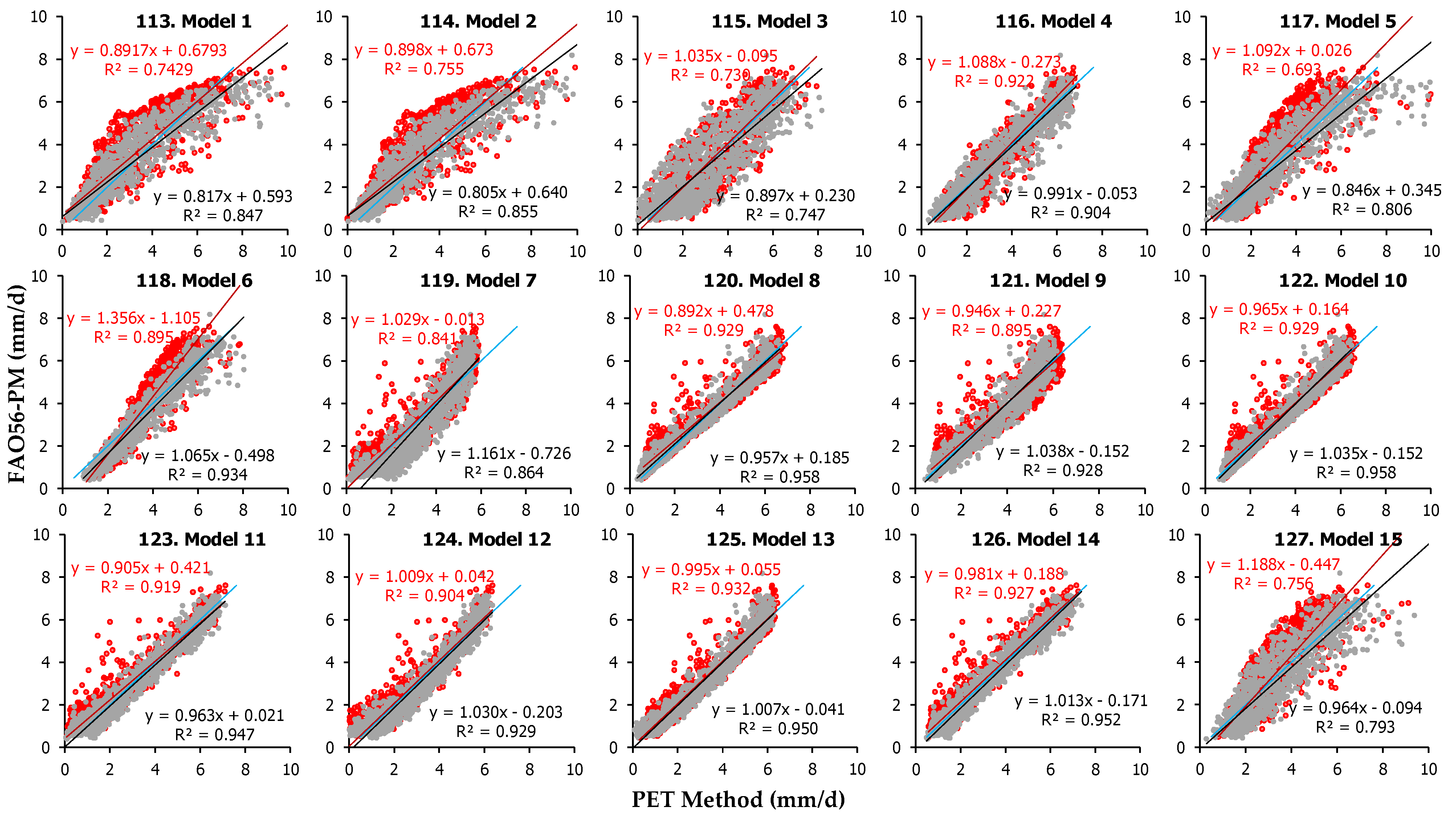
The local calibration of the empirical models for the PET estimation is suggested in most research works and is also imposed by the results of the present study. In this work, an adjustment of the general forms of mass transfer, temperature and radiation-based equations was performed for local use in the territories of our study sites. Based on the daily data from both stations, 15 adjusted PET models were produced following the general forms of several widely used equations. For example, the mass transfer model proposed by Dalton 1802 (Equation (1)), Fitzgerald 1886 (Equation (2)), Meyer 1926 (Equation (4)), Rohwer 1931 (Equation (5)), Albrecht 1950 (Equation (7)) and WMO 1966 (Equation (9)) follow the general form of PET = (a + bu) (es – ea). The adjusted values of a and b, based on the data from the two stations, are presented in Table 9. Similarly, other widely used models were adjusted for local use, and the new models are also presented in Table 9. The performance of the adjusted equations (Equations (113)–(127)) is evaluated following the estimation of statistical indices and ranking as above. The daily PET estimates for the new models are presented for the two sites along with the respective PET values by the FAO56-PM method in Figure 8.
The daily PET dispersion of values depicted in Figure 8 in association with the statistical indices of the new methods and the ranking with respect to all 127 models (112 original and 15 adjusted) in both sites that are presented in Table 10 suggest that the adjusted models performed better compared to the original equations.
More specifically, the mass transfer models 1 (Equation (113)) and 2 (Equation (114)) were ranked 66th and 64th (with sRPI scores of 0.803 and 0.813), respectively, among all 127 models, in Heraklion, whereas in Amaroussion, they performed better (ranked 42nd and 44th, with similar sRPI scores of 0.867 and 0.866, respectively). Similarly, the adjusted temperature-based models 3, 4, 5, 6 and 15 (Equations (115)–(118) and (127)) were ranked between 26th and 97th with scores ranging from 0.701 to 0.916, in Heraklion, among which model 4 performed the best (Equation (116)), which is actually an adjustment of the Hargreaves and Samani method. The temperature-based adjusted models in Amaroussion presented also good performance, and they ranked between 21st and 84th among the 127 methods, with sRPI ranging from 0.783 to 0.913, among which model 4 performed the best (Equation (116)). Finally, the radiation-based adjusted models 7–14 (Equations (119)–(126)) produced in general accurate estimates. Their sRPI scores, in Heraklion, ranged from 0.851 to 0.960, resulting in ranks varying from 4th to 50th, among which model 10 performed the best (Equation (122)). In Amaroussion, model 8 had an excellent behavior, ranking 2nd among all 127 methods, with a high sRPI value (0.972), whereas the rest of the radiation-based adjusted models also received high sRPI scores ranging from 0.819 to 0.972, with ranks varying between 7th and 67th.

4. Discussion

The PET estimates of the examined 112 models in this work confirm the overall good performance of the combination methods against all other groups of methods in the environment of the two Mediterranean urban green sites, i.e., in Heraklion (S. Greece) and Amaroussion (c. Greece). The general ranking of the methods for both sites indicate that the method of Wright 1996 (Equation (108)) performed the best followed by Valiantzas 2006 (2) (Equation (109)), Jensen et al. 1990 (Equation (106)), Valiantzas 2013 (6) (Equation (112)), Priestley and Taylor 1972 (Equation (85)), Valiantzas 2013 (4) (Equation (110)), Abtew 1996 (4) (Equation (86)), Valiantzas 2013 (5) (Equation (111)), Ahooghalaandari et al. 2017 (2) (Equation (99)) and Castañeda and Rao 2005 (2) (Equation (79)). The above ten are the best-performing methods for both sites, producing the best statistics and the highest sRPI scores (higher than 0.936).
The worst-performing methods are mainly mass transfer and temperature-based with limited data requirements. Specifically, the ten worst-performing models were Fitzgerald 1886 (Equation (2)) followed by Brockamp and Wenner 1963 (Equation (8)), Xu and Singh 2001 (5) (Equation (53)), Antal 1968 (Equation (50)), Xu and Singh 2001 (7) (Equation (55)), Tabari and Talaee 2011 (3) (Equation (94)), Schendel 1967 (Equation (49)), Dalton 1802 (Equation (1)), Blaney and Criddle 1950 (Equation (14)), and Smith and Stopp 1978 (Equation (21)), which received the minimum sRPI scores (lower than 0.590).
Regarding each category of empirical methods, the best-performing mass transfer method for both sites was Mahringer 1970 (Equation (10)), which ranked 45th among all 112 models (sRPI = 0.827). Respectively, the best temperature-based model was Ahooghalaandari et al. 2016 (3) (Equation (58)) ranking 27th (sRPI = 0.888), and the best radiation-based method was Priestley and Taylor 1972 (Equation (85)) ranking 5th (sRPI = 0.957). As mentioned above, the best-performing combination model for the two sites was Wright 1996 (Equation (108)), which ranked also first among all 112 models.
Specifically in Heraklion, the ten best-performing methods in descending order were Wright 1996 (Equation (108)), Valiantzas 2006 (2) (Equation (109)), Jensen et al. 1990, (Equation (106)), Ahooghalaandari et al. 2017 (2) (Equation (99)), Valiantzas 2013 (6) (Equation (112)), Valiantzas 2013 (4) (Equation (110), Valiantzas 2013 (5) (Equation (111)), Castañeda and Rao 2005 (2) (Equation (79)), Priestley and Taylor 1972 (Equation (85)), and Ahooghalaandari et al. 2017 (3) (Equation (100)), with sRPI scores higher than 0.939. Similarly, in Amaroussion, the ten best methods were Wright 1996 (Equation (108)), Priestley and Taylor 1972 (Equation (85)), Jensen et al. 1990 (Equation (106)), Valiantzas 2013 (6) (Equation (112)), Valiantzas 2006 (2) (Equation (109)), Abtew 1996 (4) (Equation (86)), Valiantzas 2013 (4) (Equation (110)), Valiantzas 2013 (5) (Equation (111)), Ahooghalaandari et al. 2017 (2) (Equation (99)) and Castañeda and Rao 2005 (2) (Equation (79)), with sRPI scores higher than 0.930.
The above-mentioned results confirm the generally increasing performance of empirical PET estimation methods with the number of input parameters [40] with the high data demanding combination methods to produce more accurate estimates. The performance of the radiation-based equations is adequate, and it ranked high among methods with limited data requirements. The better performance of the radiation methods compared to temperature-based is expected and has been confirmed also by Lang et al. [16], who applied different empirical PET models in southwestern China, suggesting Makkink’s model as the best alternative. In the present work, Makking’s original equation was found to perform quite well, ranking 25th among the 112 examined models with an average, for both study sites, rank score of sRPI = 0.889, whereas its modified form proposed by Castañeda and Rao 2005 (2) (Equation (79)) was ranked among the 10 best-performing methods for both examined sites and received a high sRPI score of 0.936. The good performance of the Priestley and Taylor method in this study (rank 5th/112, sRPI = 0.957) is also in line with the findings by Wei and Menzel [35], who suggested the specific method for global application.
It should be noted that the radiation-based methods requiring Rn radiation measurement are anticipated to perform better than those requiring Rs, since Rn is highly associated with the surface characteristics indicating the available energy stored in the natural surface and can be used for evapotranspiration. However, in this study, Rn is estimated from Rs [11], and thus, its effect cannot be evaluated as in the case of real in situ Rn measurements. In all cases, the best two radiation methods (included also among the 10 best out of the 112 original models) require Rn, i.e., Priestley and Taylor 1972 (Equation (85)) and Abtew 1996 (4) (Equation (86)).
The limitation of input parameters and the local calibration of the examined models appear to affect their performance in the two sites. It should be also mentioned that almost all models were established in rural areas, and thus, their application in urban environments (even in green spaces) may result in overestimations or underestimations. This is also valid for the FAO56-PM method, which is highly affected by the aerodynamic characteristics of the surface. In all cases, the energy budget and the aerodynamic characteristics of the urban green spaces are considerably different compared to the open rural areas, and the built-up urban environment highly affects the energy exchanging processes, the energy budget of the green surfaces, and the wind flow above them, resulting in a complex environment that is difficult to be modeled. Multiple radiation scattering by the built-up environment surrounding the urban green areas and shadowing, as well as the use of artificial materials covering parts of the soil, can result in decreased ET fluxes and overestimation of the applied PET models [41]. However, the estimation of PET by the empirical models remains a useful tool to assess plants’ water requirements, even at the urban environment.
The general ranking of the 127 methods (112 originals and 15 adjusted) after incorporating the scores for both sites are presented in Table A5 (Appendix C). The results suggest that many of the adjusted models performed better compared to the original equations. More specifically, the mass transfer models 1 (Equation (113)) and 2 (Equation (114)) were ranked 52nd and 51st (with sRPI scores of 0.835 and 0.839), respectively, among all 127 models, whereas the best original mass transfer method (Mahringer 1970 (Equation (10), sRPI = 0.827) is ranked 57th, WMO 1966 (Equation (9)) is ranked 59th, and all others were ranked much lower compared to the adjusted mass transfer models.
Among the adjusted temperature-based models 3, 4, 5, 6 and 15 (Equations (115)–(118) and (127)), model 4 (Equation (123)), which requires only temperature data and is actually the adjustment of the Hargreaves–Samani equation, presented better performance, ranking 22nd (sRPI = 0.915) among the 127 methods and first among all temperature-based models, which was followed by the best original method of Ahooghalaandari et al. 2016 (3) (Equation (58)), which ranked 35th/127 with sRPI = 0.888. It is worth noting the good performance of the adjusted Hargreaves–Samani Model 4 (Equation (116)) which is ranked 22nd/127, as mentioned, whereas its original form Hargreaves and Samani 1985 (Equation (22)) is ranked 86th/127 (sRPI = 0.751). It should be stated, though, that at the adjusted model 4, the power of the diurnal temperature range (DTR = Tmax − Tmin) is negative and small, suggesting a minor and negative effect of DTR on PET. Since DTR is considered to be related with atmospheric cloudiness and radiation factors that control plant photosynthesis [138,146,147] and that clear sky conditions (higher DTR) can be associated with higher evapotranspiration rates [148,149], it is rather expected for there to be a positive DTR effect on PET. On the other hand, in our two sites, clear sky conditions typically persist; thus, DTR is expected to have an overall minor effect on PET.
The radiation-based adjusted models 7–14 (Equations (119)–(126)) had sufficient performance. Models 10 (Equation (122)) and 8 (Equation (120)), which are actually adjustments of the Priestley and Taylor method with (model 10) or without (model 8) interception, presented the best performances and ranked 4th and 6th, among the 127 models with sRPI values of 0.959 and 0.957, respectively. Also, models 13 (Equation (125)), 11 (Equation (123)) and 14 (Equation (126)) are among the ten best models ranking 8th, 9th and 10th, with quite similar sRPI values: 0.957, 0.952 and 0.951, respectively. It is worth noting that model 14 (Equation (126)), namely the adjustment of the original Copais (Equation (92), has significantly improved the performance of the original method, considering that the original equation is ranked 42nd/127 (sRPI = 0.871).
All adjusted models have reduced data requirements, allowing their local application in the two study sites. Nonetheless, it should be stressed that the models’ performance will benefit from further adjustments, incorporating a longer timeseries of data from the two stations. Their application in other regions and cities should be performed with caution, following a proper validation. Furthermore, additional adjustments may be applied by incorporating data from new stations with different geographical characteristics. In any case, the local calibration can significantly improve the performance of the PET empirical models and is highly suggested especially in regions with a limited availability of meteorological data. In summary, the best-performing methods with rank scores (sRPI) higher than 0.950 (derived as average values from both study sites) are depicted in Table 11.

5. Conclusions

In the present work, the performance of 112 original empirical models for the estimation of potential evapotranspiration (PET) was investigated by comparing the models’ outputs with the PET estimates by the FAO56-PM standard method in two urban green sites in Greece (Heraklion, S. Greece and Amaroussion, c. Greece). Based on the general forms of the original mass transfer, temperature and radiation-based PET models, 15 adjusted equations were also produced and evaluated for application at the local level.
The results confirm that the accuracy of the model increases with the number of the input parameters included in the estimations. The combination methods produced in general more accurate PET estimates, which are followed by the radiation, temperature and mass transfer-based methods.
The combination model proposed by Wright 1996 (Equation (108) ranked 1st among the 112 original models) had the best performance, which was followed by Valiantzas 2006 (2) (Equation (109), ranked 2nd) and Jensen et al. 1990 (Equation (106), ranked 3rd), which are also combination methods. However, it is important to note that the combination methods require the same input parameters as FAO56-PM; thus, the standard method might be applied directly.
Priestley and Taylor (Equation (85), ranking 5th among the 112 original models) was the best radiation-based model and Ahooghalaandari et al. 2016 (3) (Equation (58), ranked 27th/112) was the best temperature-based one. Regardless of their high data requirements, the mass transfer methods had insufficient performance, even after adjustment. However, Mahringer 1970 (Equation (10), ranked 45th/112) was the best model of this category.
The adjusted PET models enhanced the performance of the original methods in all cases on the local level of the two study sites. The radiation-based model 10 (PET = f (Rs, T, RH)) was ranked 4th among all 127 models (112 original and 15 adjusted), presenting a high rank score. Also, models 8, 13, 11 and 14 (all radiation-based) produced accurate estimates in both sites, received high scores (>0.951) and ranked among the 10 best-performing methods. Their application in the two sites is recommended in the case of limited data availability; however, their applicability in other regions should be cautiously performed after proper validation and adjustment.
For wider application, it is proposed to test the methods in other cities around the world to evaluate the accuracy of the estimation of urban vegetation water requirements. It is essential though to underline the critical importance of the quality of measurements of the input parameters that should be obtained above irrigated, grass-covered surfaces, allowing the proper application of the FAO56-PM method. The findings of this study can be useful for the estimation of PET in Mediterranean cities and especially in areas with limited data availability. This can be particularly useful toward informed decision making for urban green infrastructure, including plant species selection, irrigation scheduling and water management as well as urban green management.
The findings from the present study, which is based on ground data, are a useful resource for determining the most appropriate method (especially at the local level) for estimating vegetation water requirements under the Mediterranean climate conditions. Based on the above principal information, using remote sensing—satellite data in the most appropriate PET methods identified in the two investigated sites, may produce more accurate local estimates. In future work, the performance of the PET methods can be evaluated by applying both satellite and ground data, and we can compare the methods performances. Further research is also required in order to validate the performance of the adjusted models by incorporating longer data series. In future work, the authors intend to investigate the performance of the original and adjusted models in other environments (urban or rural).
Author Contributions

Conceptualization, N.P. and D.T.; methodology, N.P., D.T. and S.G.A.; software, N.P.; validation, N.P., S.G.A., A.D.S., A.B., S.S. and S.C.N.; formal analysis, N.P., D.T. and S.G.A.; investigation, N.P., D.T., I.T., A.D.S., A.B., S.S. and S.C.N.; resources, N.P., A.D.S., A.B. and S.C.N.; data curation, N.P., D.T., I.T., S.S. and A.B.; writing—original draft preparation, N.P., D.T. and I.T.; writing—review and editing, N.P., D.T., I.T., S.G.A., A.D.S., A.B., S.S. and S.C.N.; visualization, N.P. and S.G.A.; supervision, N.P.; funding acquisition, N.P., I.T., S.G.A., S.S. and A.D.S. All authors have read and agreed to the published version of the manuscript.

Funding

This research was funded by the LIFE GrIn project “Promoting urban Integration of GReen INfrastructure to improve climate governance in cities” LIFE17GIC/GR/000029, which is co-financed by the European Commission under the Climate Change Action-Climate Change Governance and Information component of the LIFE Programme and the Greek Green Fund.

Data Availability Statement

The data presented in this study are available on request from the corresponding author.

Acknowledgments

The author acknowledge the contribution of the Municipalities of Heraklion and Amaroussion, partners of the GrIn project, for their valuable assistance in the installation and operation of the two micrometeorological stations in the green areas of their cities.

Conflicts of Interest

The authors declare no conflict of interest.

Appendix A

The statistical analysis in this work was based on the following indices:
  • Slope a, intercept b and coefficient of determination R2 of the linear regression y = ax + b.
  • Mean bias error (MBE):
    MBE = i = 1 N P i O i N
  • Mean absolute error (MAE):
    MAE = i = 1 N P i O i N
  • Differences distribution s d 2 around the MBE:
    s d 2 = i = 1 N P i O i MBE 2 N 1
  • Root mean square error (RMSE):
    RMSE = i = 1 N P i O i 2 N
  • Index of agreement (d):
    d = 1 i = 1 N P i O i 2 N i = 1 N P i + O i 2 N
    where Oi is the estimated PET by FAO56-PM, and Pi is the PET by the compared methods, P i = P i O and O i = O i O .
The ranking of the PET methods was based on the above eight indices, and the rank scores were computed by the following equations:
X i = V i   ,   Type   I   indices   R 2 ,   d 1 V i + 1 V i   max + 1   ,   Type   II   indices   1 slope   a ,   offcet   b ,   MBE ,   MAE ,   s d 2 ,   RMSE  
Y i = X i X min X max X min
RPI = i = 1 k Y i k
sRPI = RPI RPI min RPI max RPI min
where Vi is each statistical index and k is the number of the statistical indices used for the RPI and sRPI estimations.

Appendix B

Daily values of the PET estimates by all used models are presented against the respective values derived by the application of the FAO56-PM model. The results are presented by category of methods.
Figure A1. Correlation between daily PET values estimated by different mass transfer methods (x-axis) and the benchmark method of FAO56-PM (y-axis) for two urban green areas in Amaroussion (gray points) and Heraklion (red points) along with the linear regression statistics. The blue line indicates the 1:1 regression.
Remotesensing 15 03680 g0a1
Figure A2. Correlation between daily PET values estimated by different temperature-based methods (x-axis) of the general forms PET = f (T) and the benchmark method of FAO56-PM (y-axis) for two urban green areas in Amaroussion (gray points) and Heraklion (red points) along with the linear regression statistics. The blue line indicates the 1:1 regression.
Remotesensing 15 03680 g0a2
Figure A3. Correlation between daily PET values estimated by different temperature-based methods (x-axis) of the general forms PET = f (T, RH or PR) and the benchmark method of FAO56-PM (y-axis) for two urban green areas in Amaroussion (gray points) and Heraklion (red points) along with the linear regression statistics. The blue line indicates the 1:1 regression.
Remotesensing 15 03680 g0a3
Figure A4. Correlation between daily ET values estimated by different radiation-based methods (x-axis) of the general forms PET = f (Rs) and PET = f (Rs, T) with the benchmark method of FAO56-PM (y-axis) for two urban green areas in Amaroussion (gray points) and Heraklion (red points) along with the linear regression statistics. The blue line indicates the 1:1 regression.
Remotesensing 15 03680 g0a4
Figure A5. Correlation between daily ET values estimated by different radiation-based methods (x-axis) of the form PET = f (Rs, T, RH) with the benchmark method of FAO56-PM (y-axis) for two urban green areas in Amaroussion (gray points) and Heraklion (red points) along with the linear regression statistics. The blue line indicates the 1:1 regression.
Remotesensing 15 03680 g0a5
Figure A6. Correlation between daily ET values estimated by different combination methods (x-axis) and the benchmark method of FAO56-PM (y-axis) for two urban green areas in Amaroussion (gray points) and Heraklion (red points) along with the linear regression statistics. The blue line indicates the 1:1 regression.
Remotesensing 15 03680 g0a6

Appendix C

Values of the statistical indices used in the present work for the ranking of the 112 PET models. The results are presented for both study sites (Heraklion and Amaroussion) and are grouped per category of methods.
The final ranking of all examined models, including the 112 original and 15 adjusted, is also presented in the last table.
Table A1. Statistical indices (mean, slope a, intercept b, and coefficient of determination R2 of the linear regression y = ax + b, mean bias error (MBE), root mean square error (RMSE), mean absolute error (MAE), standard deviation square (sd2), and index of agreement d) and ranking (sRPI Score and Rank) based on the optimum values of the statistical indices for the 12 mass transfer-based modes (Equations (1)–(12)) for the estimation of PET compared to the benchmark method of FAO56-PM in the two urban green sites of Heraklion and Amaroussion.
PET MethodNMeanabMBERMSEMAEsd2dR2sRPIRank
Heraklion
FAO56-PM11393.266
1. Dalton 180211394.6921.2870.4911.4292.1261.5282.4770.8100.7350.603102
2. Fitzgerald 188611396.7671.9890.2743.5044.5733.5118.6340.7290.7400.177112
3. Trabert 189611393.4701.091−0.0940.2071.2700.8821.5690.9740.7380.82547
4. Meyer 192611394.5011.2070.5581.2381.9251.3602.1770.8680.7240.65495
5. Rohwer 193111394.5701.2790.3921.3072.0171.4352.3670.8900.7410.65794
6. Penman 194811394.5461.3420.1631.2802.0951.4592.7490.8910.7390.65296
7. Albrecht 195011393.6341.0800.1050.3711.2550.8301.4370.8980.7500.79656
8. Br. and Wen. 196311396.0541.876−0.0732.7913.8652.8307.1740.7150.7450.292111
9. WMO 196611392.5940.7850.025−0.6701.2120.9131.0020.9640.7290.79855
10. Mahringer 197011393.2341.015−0.087−0.0291.1580.8341.3320.9190.7380.82746
11. Szász 197311394.3250.9641.1701.0621.4221.1550.9040.8970.7900.72674
12. Linacre 199211383.6690.8950.7380.4030.9770.8010.7890.9460.7960.81352
Amaroussion
FAO56-PM11952.969
1. Dalton 180211954.9041.694−0.1211.4292.7531.9673.8280.7670.8330.547106
2. Fitzgerald 188611956.6392.410−0.5143.5044.9423.67410.9370.7640.8490.189112
3. Trabert 189611953.2251.259−0.5140.2071.1970.7861.3680.9810.8360.81756
4. Meyer 192611954.7911.630−0.0491.2382.6171.8623.5310.8300.8210.597102
5. Rohwer 193111954.6901.642−0.1851.3072.5101.7643.3410.8930.8410.63197
6. Penman 194811964.4411.617−0.3611.2802.2851.5373.0650.9060.8490.65195
7. Albrecht 195011953.6471.398−0.5060.3711.5620.9811.9850.9020.8340.74084
8. Br. and Wen. 196311955.7162.203−0.8282.7914.0032.7728.4920.7620.8440.300111
9. WMO 196611952.4650.915−0.259−0.6700.9230.6930.5920.9820.8440.85340
10. Mahringer 197011953.0051.171−0.478−0.0291.0420.7261.0850.9430.8360.82650
11. Szász 197311954.2861.3010.4171.0621.7141.3491.2220.8930.8740.73286
12. Linacre 199211873.6201.0620.4460.4031.0760.9030.7610.9570.8470.83144
Table A2. Statistical indices (mean, slope a, intercept b, and coefficient of determination R2, of the linear regression y = ax + b, mean bias error (MBE), root mean square error (RMSE), mean absolute error (MAE), standard deviation square (sd2), and index of agreement d) and ranking (sRPI Score and Rank) based on the optimum values of the statistical indices for the 48 temperature-based PET models (Equations (13)–(60)) compared to the benchmark method of FAO56-PM in the two urban green sites of Heraklion and Amaroussion.
PET MethodNMeanabMBERMSEMAEsd2DR2sRPI Rank
Heraklion
FAO56-PM11393.266
13. Thornthwaite 194811392.6520.867−0.187−0.6111.0150.7940.6310.9260.8290.83245
14. Blaney and Criddle 195011394.6370.6372.5481.3741.5821.4000.6370.7890.9040.585104
15. McCloud 195511393.3621.065−0.1260.0991.3250.9811.7350.8940.7060.78063
16. Hamon 196311392.9880.6400.887−0.2750.9190.7580.7460.9390.8450.79457
17. Baier and Robert. 196510423.0250.8230.170−0.4261.0510.8260.8940.8800.7540.78760
18. Malmstrom 196911393.4060.7580.9180.1430.8050.6670.6160.9450.8390.82249
19. Sieg. and Schrodt. 197511393.3190.6851.0690.0560.8060.6850.6310.9270.8640.80854
20. Bl. and Criddle (m. Eu.)11392.8950.6090.892−0.3680.9280.7510.6960.8770.9080.78162
21. Smith and Stopp 197811393.0670.4221.674−0.1961.2451.0691.4870.6880.7070.552108
22. Hargr. and Samani 198511392.9700.6630.788−0.2931.0500.7760.9860.8070.7370.70681
23. Kharrufa 198511394.4991.0790.9591.2361.5031.3040.7610.8410.8520.71476
24. Mintz and Walker 199311393.3560.6771.1260.0930.8150.6970.6390.9550.8660.81450
25. Camargo et al. 199911392.6180.6950.329−0.6451.2350.9721.0590.8290.7100.70780
26. Samani 200011393.1260.6830.874−0.1370.8260.6580.6350.9260.8640.81451
27. Xu and Singh 2001 (1)11393.1140.9260.068−0.1490.8690.7060.7020.9310.8210.86937
28. Xu and Singh 2001 (2)11393.1710.9340.100−0.0920.8770.7180.7310.9500.8160.87634
29. Xu and Singh 2001 (3) 11394.8991.1741.0431.6361.8991.6710.9850.8350.8520.65297
30. Xu and Singh 2001 (4)11393.6190.8070.9590.3561.0580.8810.9840.9460.7370.76766
31. Dr. and Allen 2002 (1)11393.3160.7230.9290.0530.9150.7350.8090.9270.7820.78759
32. Dr. and Allen 2002 (2)11393.1520.7070.816−0.1111.0010.7700.9560.8980.7390.75768
33. Pereira and Pruit 200411392.4740.6310.385−0.7901.3401.0571.0960.8180.7070.67886
34. Trajkovic 2005 (1)11392.9180.7630.400−0.3450.9020.7250.6440.9210.8290.82248
35. Trajcovic 2005 (2)11392.7610.5420.964−0.5021.2090.8931.1480.8230.7370.66990
36. Oudin 200511393.0130.7550.516−0.2510.7090.5780.3920.9350.9230.86938
37. Castañ. and Rao 2005 (1)11393.6020.8000.9600.3390.7430.6100.4260.9430.8930.84143
38. Trajkovic 200711392.5420.5620.676−0.7211.2790.9401.0340.8030.7750.67985
39. Tabari and Tal. 2011 (1)11394.0120.8941.0620.7481.2751.0981.0820.8470.7370.70183
40. Tabari and Tal. 2011 (2)11393.6280.8070.9590.3641.0620.8900.9850.9270.7370.75867
41. Ravazzani et al. 201211392.4990.5530.658−0.7641.3420.9801.1260.8130.7370.66591
42. Berti et al.201411392.6050.5770.684−0.6581.2750.9241.1050.8120.7280.67288
43. Heydari and Heyd. 201411392.9730.7160.598−0.2901.1040.8171.0750.8730.7050.73671
44. Dorji et al. 201611392.4030.4780.806−0.8601.4261.0731.1870.7610.8120.63999
45. Lobit et al. 201811392.4320.5170.705−0.8321.4211.0431.2210.7440.7240.617101
46. Althoff et al. 201911392.7280.6160.677−0.5351.1780.8571.0170.8370.7430.70482
47. Romanenko 196111394.5501.3740.0241.2861.9181.3492.0880.9370.8140.71575
48. Papadakis 196511394.1040.8721.2170.8411.6531.2162.0520.9060.5820.635100
49. Schendel 196711395.0371.0691.5061.7732.2141.7921.8630.8200.6930.556107
50. Antal 196811395.2321.1581.4111.9692.3921.9831.9720.8510.7220.550109
51. Linacre 197711394.6340.8811.7151.3701.6501.4140.9190.9120.7660.66093
52. Naumann 198711392.9630.8100.276−0.3001.3701.0481.7140.8840.6020.71077
53. Xu and Singh 2001 (5)11395.0561.5270.0271.7932.4611.8182.9590.7850.8140.567105
54. Xu and Singh 2001 (6)11394.5740.8701.6891.3111.5991.3660.9120.9270.7650.67189
55. Xu and Singh 2001 (7)11395.2300.9871.9621.9672.1881.9691.0540.8200.7720.563106
56. Ahoogh. et al. 2016 (1)11394.5500.8371.7691.2871.3761.2890.3140.9210.9220.72772
57. Ahoogh. et al. 2016 (2)11394.7190.8012.0581.4551.5561.4580.3960.8630.9040.66092
58. Ahoogh. et al. 2016 (3)11393.6090.9160.5690.3460.7170.5620.3790.9660.8970.88927
59. Ahoogh. et al. 2016 (4)11394.0280.9510.8740.7650.9590.8000.3620.9390.9040.83844
60. Dr. and Allen 2002 (3)11322.8080.6910.493−0.4651.3040.9711.3810.8670.6280.68984
Amaroussion
FAO56-PM11952.969
13. Thornthwaite 194811952.5780.959−0.278−0.6110.9510.7250.7450.9490.8210.83145
14. Blaney and Criddle 195011954.5520.7452.3321.3741.7251.5960.5000.8070.8880.590104
15. McCloud 195511953.3111.251−0.4120.0991.6921.1582.7520.8780.6930.68090
16. Hamon 196311952.9580.7520.714−0.2750.8190.6710.6700.9660.8250.81657
17. Baier and Robert. 196510443.4320.9780.235−0.4261.0290.8271.0330.9190.7660.79762
18. Malmstrom 196911953.3870.8950.7160.1430.9290.7450.7000.9480.8180.81755
19. Sieg. and Schrodt. 197511943.1480.7930.7790.0560.7830.6560.5870.9520.8450.82947
20. Bl. and Criddle (m. Eu.)11952.8120.7110.685−0.3680.7610.6110.5500.9390.8880.83046
21. Smith and Stopp 197811942.9020.5141.360−0.1961.1190.9591.2450.8110.7190.62898
22. Hargr. and Samani 198511953.1900.8530.643−0.2930.8680.6900.7120.9090.8110.79663
23. Kharrufa 198511944.3291.2600.5701.2361.7851.4841.3870.8510.8360.67991
24. Mintz and Walker 199311943.1840.7850.8350.0930.7930.6680.5920.9690.8470.83143
25. Camargo et al. 199911952.8900.9070.176−0.6451.0130.8081.0180.9200.7550.78370
26. Samani 200011953.1490.7910.781−0.1370.9190.6690.8200.9360.7800.78569
27. Xu and Singh 2001 (1)11952.9741.002−0.022−0.1490.9210.7370.8490.9390.8150.85737
28. Xu and Singh 2001 (2)11953.0231.0080.010−0.0920.9380.7530.8800.9510.8110.86136
29. Xu and Singh 2001 (3) 11944.7141.3710.6201.6362.1951.8321.8530.8280.8360.613100
30. Xu and Singh 2001 (4)11953.8861.0380.7830.3561.3201.0870.9420.9450.8110.78172
31. Dr. and Allen 2002 (1)11953.4870.9030.7830.0530.9390.7870.6370.9520.8370.82651
32. Dr. and Allen 2002 (2)11953.3840.9100.659−0.1110.9510.7760.7520.9410.8120.81459
33. Pereira and Pruit 200411952.7280.8340.225−0.7901.0220.8110.9730.9260.7490.76878
34. Trajkovic 2005 (1)11952.8520.8440.321−0.3450.8370.6660.6810.9460.8210.83242
35. Trajcovic 2005 (2)11952.9400.6970.845−0.5020.8810.6700.7740.9240.8110.76977
36. Oudin 200511952.8780.8310.382−0.2510.6420.5010.3990.9570.9040.88527
37. Castañ. and Rao 2005 (1)11953.5810.8770.9490.3390.8880.7430.4480.9340.8850.82253
38. Trajkovic 200711952.6850.7060.559−0.7210.8990.6340.7100.9230.8320.78866
39. Tabari and Tal. 2011 (1)11954.3081.1490.8660.7481.7151.4231.2310.8220.8110.67392
40. Tabari and Tal. 2011 (2)11953.8951.0380.7830.3641.3231.0960.9510.9330.8110.77674
41. Ravazzani et al. 201211952.7580.7320.552−0.7640.8980.6400.7480.9450.8110.78965
42. Berti et al.201411952.8050.7460.557−0.6580.8900.6420.7550.9210.8060.78171
43. Heydari and Heyd. 201411953.2610.9490.410−0.2900.9940.7760.9220.9250.7880.80560
44. Dorji et al. 201611952.4750.5780.724−0.8601.0810.7850.8890.8890.8540.74483
45. Lobit et al. 201811952.6110.6660.598−0.8320.9930.6960.8320.8710.8050.73885
46. Althoff et al. 201911952.9260.7920.537−0.5350.8500.6360.7180.9260.8130.79861
47. Romanenko 196111954.8831.933−0.8911.2862.9041.9774.9110.9140.8870.559105
48. Papadakis 196511954.7111.3210.7530.8412.4241.8212.9710.9000.7120.600101
49. Schendel 196711945.2631.6040.4601.7732.9462.3193.6010.8430.8060.531107
50. Antal 196811955.5661.5970.7861.9693.1972.6043.6790.8520.7970.489109
51. Linacre 197711954.8591.2171.2061.3702.1691.8991.2810.9140.8340.64696
52. Naumann 198711953.8771.418−0.376−0.3001.8821.2382.7930.9080.7750.69988
53. Xu and Singh 2001 (5)11955.4262.147−0.9901.7933.5732.4926.9360.8020.8870.407110
54. Xu and Singh 2001 (6)11954.7981.2031.1841.3112.1041.8391.2370.9310.8340.66294
55. Xu and Singh 2001 (7)11955.4701.3511.4181.9672.8062.5061.8340.8300.8310.518108
56. Ahoogh. et al. 2016 (1)11954.5421.0591.3531.2871.6241.5750.3020.9330.9440.74682
57. Ahoogh. et al. 2016 (2)11954.7491.0041.7241.4551.8261.7820.3280.8770.9290.68289
58. Ahoogh. et al. 2016 (3)11953.6071.1180.2400.3460.9170.7190.4930.9640.9200.88726
59. Ahoogh. et al. 2016 (4)11954.0681.1960.4720.7651.2991.1060.5810.9290.9300.81558
60. Dr. and Allen 2002 (3)11943.2130.9130.452−0.4651.0960.8631.1660.9410.7350.77076
Table A3. Statistical indices (mean, slope a, intercept b, and coefficient of determination R2, of the linear regression y = ax + b, mean bias error (MBE), root mean square error (RMSE), mean absolute error (MAE), standard deviation square (sd2), and index of agreement d) and ranking (sRPI Score and Rank) based on the optimum values of the statistical indices for the 40 radiation-based models (Equations (61)–(100)) for the estimation of PET compared to the benchmark method of FAO56-PM in the two urban green sites of Heraklion and Amaroussion.
PET MethodNMeanabMBERMSEMAEsd2DR2sRPI Rank
Heraklion
FAO56-PM11393.266
61. Christiansen 196811392.6570.6680.423−0.6071.0940.8800.7110.8840.8410.77564
62. Abtew 1996 (1)11393.5700.9030.5710.3070.8450.7060.5980.9350.8410.84642
63. Makkink 195711382.8060.849−0.021−0.4600.8350.6730.3800.9440.8990.88629
64. Stephens and Stewart 196311392.6590.898−0.329−0.6050.8770.7420.2790.9430.9250.87833
65. Jensen and Haise 196311394.2191.471−0.6400.9561.5191.2601.4440.8970.9260.72773
66. Stephens 196511354.1811.670−1.3420.9091.8261.4282.5560.9210.9170.64498
67. McGuinness and Bordne 197211392.6590.898−0.329−0.6040.8800.7470.2790.9500.9250.88031
68. Ritchie 197211393.6711.0840.0760.4080.8200.7160.4940.9580.9020.89824
69. Caprio 197411394.0531.450−0.7400.7901.3951.1491.3560.9270.9260.75370
70. Hargreaves 197511393.6411.137−0.1290.3780.8120.7160.5010.9760.9160.90222
71. Hansen 198411393.3530.9740.1120.0900.6720.5540.3930.9750.8990.93412
72. de Bruin 198711393.1190.9050.104−0.1440.6870.5460.3700.9760.8990.92414
73. Wendling 1991–199511393.4660.9750.2200.2030.6920.5820.3990.9670.8980.91917
74. Abtew 1996 (2)11393.3800.8760.4570.1170.7050.5900.4340.9650.8820.89126
75. Abtew 1996 (3)11393.1651.065−0.376−0.0990.7470.6060.4690.9670.9020.90719
76. Irmak et al. 2003 (1)11383.4330.8360.6390.1680.6880.5860.4010.9650.8950.88032
77. Irmak et al. 2003 (2)10474.8461.467−0.2921.3951.8511.6411.6120.8540.9000.67687
78. Irmak et al. 2003 (3)11234.8991.4440.0711.6031.9451.7301.3660.9100.9210.70978
79. Castañeda and Rao 2005 (2)11383.2430.974−0.007−0.0220.6830.5530.3940.9790.8990.9438
80. Valiantzas 2013 (1)11373.4481.0090.0820.1820.7340.6340.4600.9660.8910.92215
81. Tabari et al. 2013 (1)11333.0020.8230.234−0.2750.8210.6770.4880.9510.8690.87235
82. Tabari et al. 2013 (2)11343.0210.8040.317−0.2520.7470.6020.3860.9510.9070.88430
83. Ahooghalaan. et al. 2017 (1)11373.5760.9170.5080.3110.8540.7550.6050.9410.8420.85141
84. Turc 196111393.5170.9860.2250.2530.6680.5690.3460.9710.9130.92613
85. Priestley and Taylor 197211393.2491.058−0.279−0.0140.6390.4990.3320.9860.9290.9419
86. Abtew 1996 (4)11393.0480.991−0.261−0.2150.6600.4860.2810.9690.9290.93511
87. Xu and Singh 20008392.2620.799−1.012−1.7051.9231.9120.3310.6910.9050.603103
88. Irmak et al. 2003 (4)11393.5560.8070.8450.2920.7000.6120.3730.9550.9110.86239
89. Irmak et al. 2003 (5)11394.5811.3740.0181.3181.6301.4071.0470.9320.9280.76965
90. Irmak et al. 2003 (6)11394.6551.3710.1001.3911.6821.4651.0330.9220.9290.75569
91. Berengena and Gavilán 200511394.2371.386−0.3650.9741.4001.1651.0860.9440.9290.78361
92. Copais11393.7551.140−0.0460.4920.8830.7570.5370.9580.9120.88828
93. Valiantzas 2006 (1)11393.8091.0790.2070.5460.7140.6300.2190.9740.9570.92116
94. Tabari and Talaee 2011 (3)11395.4741.797−0.4742.2112.7992.2763.2260.7750.9290.495110
95. Tabari and Talaee 2011 (4)11394.6691.529−0.4031.4051.8721.5361.6790.9370.9290.70879
96. Valiantzas 2013 (2)11393.8511.1170.1230.5880.8280.7410.3540.9650.9380.90023
97. Valiantzas 2013 (3)11393.8931.1650.0060.6300.8450.7200.3390.9660.9550.90420
98. Milly and Dunne 201611392.9690.8500.109−0.2940.7870.6100.3970.9740.8950.90321
99. Ahooghalaan. et al. 2017 (2)11393.5180.9770.2430.2550.5340.4160.1780.9840.9540.9554
100. Ahooghalaan. et al. 2017 (3)11393.5520.9800.2660.2890.5980.4930.2370.9760.9390.93910
Amaroussion
FAO56-PM11952.969
61. Christiansen 196811952.6500.6080.795−0.6070.9760.7840.8190.9070.8640.76879
62. Abtew 1996 (1)11953.5620.8221.0730.3070.9200.7790.5530.9030.8640.78668
63. Makkink 195711932.7600.8070.311−0.4600.6500.5300.3560.9590.9340.89225
64. Stephens and Stewart 196311952.5660.883−0.106−0.6050.6880.5740.2700.9590.9450.90720
65. Jensen and Haise 196311954.0631.452−0.3010.9561.5311.2181.2620.8910.9430.76680
66. Stephens 196511554.0731.681−1.0870.9091.9091.4282.6850.9150.9140.66993
67. McGuinness and Bordne 197211952.5670.882−0.106−0.6040.6920.5790.2730.9660.9450.91018
68. Ritchie 197211953.6911.0370.5580.4081.0620.8100.6850.9250.8630.82552
69. Caprio 197411953.8861.439−0.4430.7901.4101.1031.2480.9250.9390.78667
70. Hargreaves 197511953.5531.0960.2440.3780.7870.6940.3430.9770.9460.91017
71. Hansen 198411953.2990.9270.4910.0900.6090.5220.3010.9770.9340.91612
72. de Bruin 198711953.0680.8600.456−0.1440.5660.4690.3230.9840.9340.91613
73. Wendling 1991–199511953.4290.9260.6210.2030.6810.5910.3070.9630.9330.89424
74. Abtew 1996 (2)11953.3570.8510.7710.1170.7140.6100.4060.9610.9100.86932
75. Abtew 1996 (3)11953.2011.098−0.121−0.0990.7330.6080.5110.9670.9140.91116
76. Irmak et al. 2003 (1)11923.3520.8220.8460.1680.6900.5950.3800.9590.9250.86733
77. Irmak et al. 2003 (2)11034.6611.4420.0551.3951.8321.6331.2690.8520.9350.72087
78. Irmak et al. 2003 (3)11804.5071.3700.3391.6031.7071.5550.8250.9250.9630.75881
79. Castañeda and Rao 2005 (2)11943.1880.9260.373−0.0220.5720.4860.3080.9840.9340.93010
80. Valiantzas 2013 (1)11853.4191.0020.3610.1820.7270.6340.3990.9640.9170.90521
81. Tabari et al. 2013 (1)11832.9740.7720.599−0.2750.7020.5900.4900.9610.9030.86335
82. Tabari et al. 2013 (2)11902.8980.7640.556−0.2520.6440.5310.3980.9560.9450.88528
83. Ahooghalaan. et al. 2017 (1)11863.6060.9670.6510.3110.9500.8360.6010.9260.8660.82848
84. Turc 196111943.4971.0420.3320.2530.7340.6290.3340.9690.9400.91215
85. Priestley and Taylor 197211953.0271.018−0.065−0.0140.4860.3750.2410.9920.9580.9722
86. Abtew 1996 (4)11952.8410.954−0.061−0.2150.5130.3740.2290.9790.9580.9566
87. Xu and Singh 20008612.1160.767−0.865−1.7051.8431.8400.3790.7020.9320.62199
88. Irmak et al. 2003 (4)11953.3680.7790.9830.2920.7010.6400.3900.9520.9420.85439
89. Irmak et al. 2003 (5)11934.2441.3660.1101.3181.5311.3250.9120.9330.9510.79364
90. Irmak et al. 2003 (6)11934.3301.3620.2081.3911.5951.3990.9020.9260.9510.77773
91. Berengena and Gavilán 200511953.9471.333−0.0850.9741.2561.0350.7650.9510.9580.83941
92. Copais11953.8591.2050.2060.4921.1280.9750.6140.9400.9330.85438
93. Valiantzas 2006 (1)11953.7281.1880.1250.5460.9080.7780.3630.9660.9710.90123
94. Tabari and Talaee 2011 (3)11955.1001.729−0.1102.2112.5882.1442.4830.7880.9580.591103
95. Tabari and Talaee 2011 (4)11954.3501.471−0.0931.4051.7101.4131.2300.9420.9580.77575
96. Valiantzas 2013 (2)11943.8151.1860.2130.5881.0270.9030.4730.9550.9510.87331
97. Valiantzas 2013 (3)11953.8521.287−0.0480.6301.1080.9130.5860.9520.9680.87330
98. Milly and Dunne 201611952.7830.8040.316−0.2940.6870.5060.4080.9770.9280.90222
99. Ahooghalaan. et al. 2017 (2)11953.4741.158−0.0450.2550.7310.5620.3610.9780.9640.9339
100. Ahooghalaan. et al. 2017 (3)11943.5481.1020.1920.2890.7850.6630.3770.9700.9460.91314
Table A4. Statistical indices (mean, slope a, intercept b, and coefficient of determination R2, of the linear regression y = ax + b, mean bias error (MBE), root mean square error (RMSE), mean absolute error (MAE), standard deviation square (sd2), and index of agreement d) and ranking (sRPI Score and Rank) based on the optimum values of the statistical indices for the 12 combination models (Equations (101)–(112)) for the estimation of PET compared to the benchmark method of FAO56-PM in the two urban green sites of Heraklion and Amaroussion.
PET MethodNMeanabMBERMSEMAEsd2DR2sRPI Rank
Heraklion
FAO56-PM11393.266
101. Penman 196311393.9591.1120.2400.6950.7270.6950.0790.9690.9940.91818
102. Kimberly Penman 197211394.2331.2050.2120.9701.0250.9700.1920.9520.9940.86936
103. mod. Makkink (Door. and Pruitt 1977)11273.9321.327−0.5240.6421.1200.9880.8680.9410.9310.81353
104. FAO24 Penman11394.2981.2010.2881.0351.0731.0350.1780.9530.9960.86140
105. FAO24 Radiation11274.0941.370−0.5070.8041.2601.1190.9970.9420.9320.79258
106. Jensen et al. 199011393.6291.104−0.0670.3650.5240.3770.1160.9890.9850.9633
107. Linacre 199310953.6361.219−0.5580.2760.7040.6410.3750.9750.9640.89625
108. Wright 199611393.2391.005−0.134−0.0240.4460.3150.0990.9890.9760.9871
109. Valiantzas 2006 (2)11393.6151.081−0.0080.3520.4790.4110.0780.9860.9900.9702
110. Valiantzas 2013 (4)11383.5901.120−0.1640.3240.5530.4990.1670.9830.9770.9476
111. Valiantzas 2013 (5)11393.6121.156−0.2570.3490.5480.4460.1490.9850.9900.9437
112. Valiantzas 2013 (6)11363.2511.016−0.170−0.0170.6040.4880.2630.9790.9370.9545
Amaroussion
FAO56-PM11952.969
101. Penman 196311953.7221.1400.2550.6950.8020.7550.2000.9680.9920.90819
102. Kimberly Penman 197211953.8681.2120.1870.9700.9650.9010.2720.9580.9970.88329
103. mod. Makkink (Door. and Pruitt 1977)11813.9511.349−0.1760.6421.2661.0920.8540.9240.9530.82849
104. FAO24 Penman11953.9821.2250.2601.0351.0751.0150.3000.9530.9960.86534
105. FAO24 Radiation11834.0761.375−0.1260.8041.3811.2040.9220.9340.9550.81954
106. Jensen et al. 199011953.3361.0930.0030.3650.5290.3700.2090.9880.9820.9633
107. Linacre 199311523.4361.155−0.1810.2760.6680.6080.3690.9760.9630.92411
108. Wright 199611952.9980.984−0.010−0.0240.3930.2640.1590.9910.9830.9921
109. Valiantzas 2006 (2)11953.3911.114−0.0060.3520.5280.4430.1760.9830.9930.9625
110. Valiantzas 2013 (4)11943.3611.0990.0070.3240.5700.5130.2440.9820.9760.9527
111. Valiantzas 2013 (5)11953.3381.165−0.2130.3490.5460.4290.2290.9840.9940.9478
112. Valiantzas 2013 (6)11853.0980.9690.110−0.0170.5020.4220.2600.9850.9570.9624
Table A5. Ranking of all 127 models (112 original and 15 adjusted).
PET MethodCategoryFormsRPIRank
108. Wright 1996CombinationPET = f (Rs, u, T, RH)0.9901
109. Valiantzas 2006 (2)CombinationPET = f (Rs, u, T, RH)0.9662
106. Jensen et al. 1990CombinationPET = f (Rs, u, T, RH)0.9633
122. Model 10Radiation-basedPET = f (Rs, T, RH)0.9594
112. Valiantzas 2013 (6)CombinationPET = f (Rs, u, T)0.9585
120. Model 8Radiation-basedPET =f (Rs, T, RH)0.9576
85. Priestley and Taylor 1972Radiation-basedPET = f (Rs, T, RH)0.9577
125. Model 13Radiation-basedPET = f (Rs, T)0.9578
123. Model 11Radiation-basedPET = f (Rs, T)0.9529
126. Model 14Radiation-basedPET = f (Rs, T, RH)0.95110
110. Valiantzas 2013 (4)CombinationPET = f (Rs, u, T, RH)0.95011
86. Abtew 1996 (4)Radiation-basedPET = f (Rs, T, RH)0.94512
111. Valiantzas 2013 (5)CombinationPET = f (Rs, u, T, RH)0.94513
99. Ahooghalaandari et al. 2017 (2)Radiation-basedPET = f (Rs, T, RH)0.94414
79. Castañeda and Rao 2005 (2)Radiation-basedPET = f (Rs, T)0.93615
121. Model 9Radiation-basedPET = f (Rs, T)0.93116
100. Ahooghalaandari et al. 2017 (3)Radiation-basedPET = f (Rs, T, RH)0.92617
124. Model 12Radiation-basedPET = f (Rs, T)0.92518
71. Hansen 1984Radiation-basedPET = f (Rs, T)0.92519
72. de Bruin 1987Radiation-basedPET = f (Rs, T)0.92020
84. Turc 1961Radiation-basedPET = f (Rs, T, RH)0.91921
116. Model 4Temperature-basedPET = f (T)0.91522
80. Valiantzas 2013 (1)Radiation-basedPET = f (Rs, T)0.91323
101. Penman 1963CombinationPET = f (Rs, u, T, RH)0.91324
93. Valiantzas 2006 (1)Radiation-basedPET = f (Rs, T, RH)0.91125
107. Linacre 1993CombinationPET = f (Rs, u, T, RH)0.91026
75. Abtew 1996 (3)Radiation-basedPET = f (Rs, T)0.90927
73. Wendling 1991–1995Radiation-basedPET = f (Rs, T)0.90628
70. Hargreaves 1975Radiation-basedPET = f (Rs, T)0.90629
98. Milly and Dunne 2016Radiation-basedPET = f (Rs, T, RH)0.90230
67. McGuinness and Bordne 1972Radiation-basedPET = f (Rs, T)0.89531
64. Stephens and Stewart 1963Radiation-basedPET = f (Rs, T)0.89232
63. Makkink 1957Radiation-basedPET = f (Rs, T)0.88933
97. Valiantzas 2013 (3)Radiation-basedPET = f (Rs, T, RH)0.88834
58. Ahooghalaandari et al. 2016 (3)Temperature-basedPET = f (T, RH)0.88835
96. Valiantzas 2013 (2)Radiation-basedPET = f (Rs, T, RH)0.88636
82. Tabari et al. 2013 (2)Radiation-basedPET = f (Rs, T)0.88437
74. Abtew 1996 (2)Radiation-basedPET = f (Rs, T)0.88038
36. Oudin 2005Temperature-basedPET = f (T)0.87739
102. Kimberly Penman 1972CombinationPET = f (Rs, u, T, RH)0.87640
76. Irmak et al. 2003 (1)Radiation-basedPET = f (Rs, T)0.87441
92. CopaisRadiation-basedPET = f (Rs, T, RH)0.87142
28. Xu and Singh 2001 (2)Temperature-basedPET = f (T)0.86943
81. Tabari et al. 2013 (1)Radiation-basedPET = f (Rs, T)0.86744
104. FAO24 PenmanCombinationPET = f (Rs, u, T, RH)0.86345
27. Xu and Singh 2001 (1)Temperature-basedPET = f (T)0.86346
68. Ritchie 1972Radiation-basedPET = f (Rs, T)0.86147
118. Model 6Temperature-basedPET = f (T,RH)0.86048
88. Irmak et al. 2003 (4)Radiation-basedPET = f (Rs, T, RH)0.85849
83. Ahooghalaandari et al. 2017 (1)Radiation-basedPET = f (Rs, T)0.83950
114. Model 2Mass transfer-basedPET = f (u,T,RH)0.83951
113. Model 1Mass transfer-basedPET = f (u,T,RH)0.83552
119. Model 7Radiation-basedPET = f (Rs)0.83553
13. Thornthwaite 1948Temperature-basedPET = f (T)0.83154
37. Castañeda and Rao 2005 (1)Temperature-basedPET = f (T)0.83155
34. Trajkovic 2005 (1)Temperature-basedPET = f (T)0.82756
10. Mahringer 1970Mass transfer-basedPET = f (u, T, RH)0.82757
59. Ahooghalaandari et al. 2016 (4)Temperature-basedPET = f (T, RH)0.82658
9. WMO 1966Mass transfer-basedPET = f (u, T, RH)0.82659
24. Mintz and Walker 1993Temperature-basedPET = f (T)0.82360
12. Linacre 1992Mass transfer-basedPET = f (u, T, RH)0.82261
3. Trabert 1896Mass transfer-basedPET = f (u, T, RH)0.82162
103. mod. Makkink (Doorenbos and Pruitt 1977)CombinationPET = f (Rs, u, T, RH)0.82063
18. Malmstrom 1969Temperature-basedPET = f (T)0.82064
19. Siegert and Schrodter 1975Temperature-basedPET = f (T)0.81865
62. Abtew 1996 (1)Radiation-basedPET = f (Rs)0.81666
91. Berengena and Gavilán 2005Radiation-basedPET = f (Rs, T, RH)0.81167
31. Droogers and Allen 2002 (1)Temperature-basedPET = f (T)0.80668
105. FAO24 RadiationCombinationPET = f (Rs, u, T, RH)0.80669
20. Blaney and Criddle (Mid. Europ. Ver.)Temperature-basedPET = f (T)0.80570
16. Hamon 1963Temperature-basedPET = f (T)0.80571
26. Samani 2000Temperature-basedPET = f (T)0.80072
17. Baier and Robertson 1965Temperature-basedPET = f (T)0.79273
32. Droogers and Allen 2002 (2)Temperature-basedPET = f (T)0.78674
89. Irmak et al. 2003 (5)Radiation-basedPET = f (Rs, T, RH)0.78175
30. Xu and Singh 2001 (4)Temperature-basedPET = f (T)0.77476
61. Christiansen 1968Radiation-basedPET = f (Rs)0.77277
43. Heydari and Heydari 2014Temperature-basedPET = f (T)0.77078
69. Caprio 1974Radiation-basedPET = f (Rs, T)0.76979
115. Model 3Temperature-basedPET =f (T)0.76980
127. Model 15Radiation-basedPET = f (T, RH)0.76981
117. Model 5Temperature-basedPET = f (T,RH)0.76882
7. Albrecht 1950Mass transfer-basedPET = f (u, T, RH)0.76883
40. Tabari and Talaee 2011 (2)Temperature-basedPET = f (T)0.76784
90. Irmak et al. 2003 (6)Radiation-basedPET = f (Rs, T, RH)0.76685
22. Hargreaves and Samani 1985Temperature-basedPET = f (T)0.75186
46. Althoff et al. 2019Temperature-basedPET = f (T)0.75187
65. Jensen and Haise 1963Radiation-basedPET = f (Rs, T)0.74688
25. Camargo et al. 1999Temperature-basedPET = f (T)0.74589
95. Tabari and Talaee 2011 (4)Radiation-basedPET = f (Rs, T, RH)0.74290
56. Ahooghalaandari et al. 2016 (1)Temperature-basedPET = f (T, RH)0.73791
78. Irmak et al. 2003 (3)Radiation-basedPET = f (Rs, T)0.73492
38. Trajkovic 2007Temperature-basedPET = f (T)0.73393
15. McCloud 1955Temperature-basedPET = f (T)0.73094
60. Droogers and Allen 2002 (3)Temperature-basedPET = f (T, PR)0.72995
11. Szász 1973Mass transfer-basedPET = f (u, T, RH)0.72996
41. Ravazzani et al. 2012Temperature-basedPET = f (T)0.72797
42. Berti et al.2014Temperature-basedPET = f (T)0.72798
33. Pereira and Pruit 2004Temperature-basedPET = f (T)0.72399
35. Trajcovic 2005 (2)Temperature-basedPET = f (T)0.719100
52. Naumann 1987Temperature-basedPET = f (T, RH)0.704101
77. Irmak et al. 2003 (2)Radiation-basedPET = f (Rs, T)0.698102
23. Kharrufa 1985Temperature-basedPET = f (T)0.697103
44. Dorji et al. 2016Temperature-basedPET = f (T)0.691104
39. Tabari and Talaee 2011 (1)Temperature-basedPET = f (T)0.687105
45. Lobit et al. 2018Temperature-basedPET = f (T)0.678106
57. Ahooghalaandari et al. 2016 (2)Temperature-basedPET = f (T, RH)0.671107
54. Xu and Singh 2001 (6)Temperature-basedPET = f (T, RH)0.667108
66. Stephens 1965Radiation-basedPET = f (Rs, T)0.656109
51. Linacre 1977Temperature-basedPET = f (T, RH)0.653110
6. Penman 1948Mass transfer-basedPET = f (u, T, RH)0.651111
5. Rohwer 1931Mass transfer-basedPET = f (u, T, RH)0.644112
47. Romanenko 1961Temperature-basedPET = f (T, RH)0.637113
29. Xu and Singh 2001 (3) Temperature-basedPET = f (T)0.632114
4. Meyer 1926Mass transfer-basedPET = f (u, T, RH)0.626115
48. Papadakis 1965Temperature-basedPET = f (T, RH)0.617116
87. Xu and Singh 2000Radiation-basedPET = f (Rs, T, RH)0.612117
21. Smith and Stopp 1978Temperature-basedPET = f (T)0.590118
14. Blaney and Criddle 1950Temperature-basedPET = f (T)0.588119
1. Dalton 1802Mass transfer-basedPET = f (u, T, RH)0.575120
49. Schendel 1967Temperature-basedPET = f (T, RH)0.543121
94. Tabari and Talaee 2011 (3)Radiation-basedPET = f (Rs, T, RH)0.543122
55. Xu and Singh 2001 (7)Temperature-basedPET = f (T, RH)0.540123
50. Antal 1968Temperature-basedPET = f (T, RH)0.519124
53. Xu and Singh 2001 (5)Temperature-basedPET = f (T, RH)0.487125
8. Brockamp and Wenner 1963Mass transfer-basedPET = f (u, T, RH)0.296126
2. Fitzgerald 1886Mass transfer-basedPET = f (u, T, RH)0.183127

References

  1. Ha, W.; Kolb, T.E.; Springer, A.E.; Dore, S.; O’Donnell, F.C.; Morales, R.M.; Lopez, S.M.; Koch, G.W. Evapotranspiration comparisons between eddy covariance measurements and meteorological and remote-sensing-based models in disturbed ponderosa pine forests. Ecohydrology 2015, 8, 1335–1350. [Google Scholar] [CrossRef]
  2. Wang, K.; Dickinson, R.E. A review of global terrestrial evapotranspiration: Observation, modeling, climatology, and climatic variability. Rev. Geophys. 2012, 50, RG2005. [Google Scholar] [CrossRef]
  3. Xu, M.; Ma, Q.; Li, S.; Yang, F.; Zhang, T.; Xu, F.; Yang, B.; Zhang, H.; Zhang, S.; Wang, Q.; et al. The estimation and partitioning of evapotranspiration in a coniferous plantation in subtropical China. Front. Plant Sci. 2023, 14, 1120202. [Google Scholar] [CrossRef] [PubMed]
  4. Jung, M.; Reichstein, M.; Ciais, P.; Seneviratne, S.I.; Sheffield, J.; Goulden, M.L.; Bonan, G.; Cescatti, A.; Chen, J.; De Jeu, R.; et al. Recent decline in the global land evapotranspiration trend due to limited moisture supply. Nature 2010, 467, 951–954. [Google Scholar] [CrossRef] [PubMed] [Green Version]
  5. Boast, C.; Robertson, T. A “micro-lysimeter” method for determining evaporation from bare soil: Description and laboratory evaluation. Soil Sci. Soc. Am. J. 1982, 46, 689–696. [Google Scholar] [CrossRef]
  6. Oishi, A.C.; Oren, R.; Novick, K.A.; Palmroth, S.; Katul, G.G. Interannual invariability of forest evapotranspiration and its consequence to water flow downstream. Ecosystems 2010, 13, 421–436. [Google Scholar] [CrossRef]
  7. Xu, M.; Wen, X.; Wang, H.; Zhang, W.; Dai, X.; Song, J.; Wang, Y.; Fu, X.; Liu, Y.; Sun, X.; et al. Effects of climatic factors and ecosystem responses on the inter-annual variability of evapotranspiration in a coniferous plantation in subtropical China. PLoS ONE 2014, 9, e85593. [Google Scholar] [CrossRef] [Green Version]
  8. Alexandris, S.; Proutsos, N. How significant is the effect of the surface characteristics on the Reference Evapotranspiration estimates? Agric. Water Manag. 2020, 237, 106181. [Google Scholar] [CrossRef]
  9. Tegos, A.; Stefanidis, S.; Cody, J.; Koutsoyiannis, D. On the Sensitivity of Standardized-Precipitation-Evapotranspiration and Aridity Indexes Using Alternative Potential Evapotranspiration Models. Hydrology 2023, 10, 64. [Google Scholar] [CrossRef]
  10. Raza, A.; Al-Ansari, N.; Hu, Y.; Acharki, S.; Vishwakarma, D.K.; Aghelpour, P.; Zubair, M.; Wandolo, C.A.; Elbeltagi, A. Misconceptions of Reference and Potential Evapotranspiration: A PRISMA-Guided Comprehensive Review. Hydrology 2022, 9, 153. [Google Scholar] [CrossRef]
  11. Allen, R.G.; Pereira, L.S.; Raes, D.; Smith, M. Crop evapotranspiration-Guidelines for computing crop water requirements-FAO Irrigation and drainage paper 56. FAO Rome 1998, 300, D05109. [Google Scholar]
  12. Allen, R.G.; Pereira, L.S.; Smith, M.; Raes, D.; Wright, J.L. FAO-56 dual crop coefficient method for estimating evaporation from soil and application extensions. J. Irrig. Drain. Eng. 2005, 131, 2–13. [Google Scholar] [CrossRef] [Green Version]
  13. Allen, R.G.; Pruitt, W.O.; Wright, J.L.; Howell, T.A.; Ventura, F.; Snyder, R.; Itenfisu, D.; Steduto, P.; Berengena, J.; Yrisarry, J.B.; et al. A recommendation on standardized surface resistance for hourly calculation of reference ETo by the FAO56 Penman-Monteith method. Agric. Water Manag. 2006, 81, 1–22. [Google Scholar] [CrossRef]
  14. Bourletsikas, A.; Argyrokastritis, I.; Proutsos, N. Comparative evaluation of 24 reference evapotranspiration equations applied on an evergreen-broadleaved forest. Hydrol. Res. 2018, 49, 1028–1041. [Google Scholar] [CrossRef]
  15. Da Silva, H.; dos Santos, M.S.; Junior, J.B.C.; Spyrides, M. Modeling of reference evapotranspiration by multiple linear regression. J. Hyperspectral Remote Sens. 2016, 6, 44–58. [Google Scholar] [CrossRef]
  16. Lang, D.; Zheng, J.; Shi, J.; Liao, F.; Ma, X.; Wang, W.; Chen, X.; Zhang, M. A comparative study of potential evapotranspiration estimation by eight methods with FAO Penman–Monteith method in southwestern China. Water 2017, 9, 734. [Google Scholar] [CrossRef] [Green Version]
  17. Wang, J.; Georgakakos, K.P. Estimation of potential evapotranspiration in the mountainous Panama Canal watershed. Hydrol. Process. Int. J. 2007, 21, 1901–1917. [Google Scholar] [CrossRef]
  18. Doorenbos, J.; Pruitt, W. Guidelines for Predicting Crop Water Requirements; FAO Irrigation and Drainage Paper No. 24; Food and Agriculture Organization: Rome, Italy, 1975; p. 179. [Google Scholar]
  19. Doorenbos, J.; Pruitt, W. Crop Water Requirements; FAO Irrigation and Drainage Paper 24; Land and Water Development Division, FAO: Rome, Italy, 1977; p. 144. [Google Scholar]
  20. Pruitt, W.; Doorenbos, J. Empirical Calibration: A Requisite for Evapotranspiration Formulae Based on Daily or Longer Mean Climate Data? International Committee on Irrigation and Drainage: Budapest, Hungary, 1977. [Google Scholar]
  21. Jensen, M.E.; Burman, R.D.; Allen, R.G. Evapotranspiration and irrigation water requirements. In Manuals and Report on Engruppe Practice; America Society Civil Engrs (ASCE): New York, NY, USA, 1990; Volume 70. [Google Scholar]
  22. Wright, J.L. New evapotranspiration crop coefficients. J. Irrig. Drain. Div. 1982, 108, 57–74. [Google Scholar] [CrossRef]
  23. Wright, J.L. Derivation of Alfalfa and Grass Reference Evapotranspiration; U.S. Department of Agriculture: Washington, DC, USA, 1996; pp. 133–140.
  24. Wright, J.L.; Jensen, M.E. Peak water requirements of crops in southern Idaho. J. Irrig. Drain. Div. 1972, 98, 193–201. [Google Scholar] [CrossRef]
  25. Coleman, G.; DeCoursey, D.G. Sensitivity and model variance analysis applied to some evaporation and evapotranspiration models. Water Resour. Res. 1976, 12, 873–879. [Google Scholar] [CrossRef]
  26. Saxton, K.E. Sensitivity analyses of the combination evapotranspiration equation. Agric. Meteorol. 1975, 15, 343–353. [Google Scholar] [CrossRef]
  27. Irmak, S.; Payero, J.O.; Martin, D.L.; Irmak, A.; Howell, T.A. Sensitivity analyses and sensitivity coefficients of standardized daily ASCE-Penman-Monteith equation. J. Irrig. Drain. Eng. 2006, 132, 564–578. [Google Scholar] [CrossRef]
  28. Gong, L.; Xu, C.-Y.; Chen, D.; Halldin, S.; Chen, Y.D. Sensitivity of the Penman–Monteith reference evapotranspiration to key climatic variables in the Changjiang (Yangtze River) basin. J. Hydrol. 2006, 329, 620–629. [Google Scholar] [CrossRef]
  29. Schendel, U. Vegetationswasserverbrauch und-wasserbedarf. Habilit. Kiel 1967, 137, 1–11. [Google Scholar]
  30. Baier, W.; Robertson, G.W. Estimation of latent evaporation from simple weather observations. Can. J. Plant Sci. 1965, 45, 276–284. [Google Scholar] [CrossRef]
  31. Trajkovic, S. Hargreaves versus Penman-Monteith under humid conditions. J. Irrig. Drain. Eng. 2007, 133, 38–42. [Google Scholar] [CrossRef]
  32. Shirmohammadi-Aliakbarkhani, Z.; Saberali, S.F. Evaluating of eight evapotranspiration estimation methods in arid regions of Iran. Agric. Water Manag. 2020, 239, 106243. [Google Scholar] [CrossRef]
  33. Tukimat, N.N.A.; Harun, S.; Shahid, S. Comparison of different methods in estimating potential evapotranspiration at Muda Irrigation Scheme of Malaysia. J. Agric. Rural Dev. Trop. Subtrop. JARTS 2012, 113, 77–85. [Google Scholar]
  34. Lu, J.; Sun, G.; McNulty, S.G.; Amatya, D.M. A comparison of six potential evapotranspiration methods for regional use in the southeastern United States 1. JAWRA J. Am. Water Resour. Assoc. 2005, 41, 621–633. [Google Scholar] [CrossRef]
  35. Weiß, M.; Menzel, L. A global comparison of four potential evapotranspiration equations and their relevance to stream flow modelling in semi-arid environments. Adv. GeoSci. 2008, 18, 15–23. [Google Scholar] [CrossRef] [Green Version]
  36. Chen, D.; Gao, G.; Xu, C.-Y.; Guo, J.; Ren, G. Comparison of the Thornthwaite method and pan data with the standard Penman-Monteith estimates of reference evapotranspiration in China. Clim. Res. 2005, 28, 123–132. [Google Scholar] [CrossRef]
  37. Nikam, B.R.; Kumar, P.; Garg, V.; Thakur, P.K.; Aggarwal, S. Comparative evaluation of different potential evapotranspiration estimation approaches. Int. J. Resour. Eng. Technol. 2014, 3, 543–552. [Google Scholar]
  38. Gupta, H.V.; Sorooshian, S.; Yapo, P.O. Status of automatic calibration for hydrologic models: Comparison with multilevel expert calibration. J. Hydrol. Eng. 1999, 4, 135–143. [Google Scholar] [CrossRef]
  39. Toriman, M.E.; Mokhtar, M.; Gasim, M.B.; Abdullah, S.M.S.; Jaafar, O.; Abd Aziz, N.A. Water resources study and modeling at North Kedah: A case of Kubang Pasu and Padang Terap water supply schemes. Res. J. Earth Sci. 2009, 1, 35–42. [Google Scholar]
  40. Bogawski, P.; Bednorz, E. Comparison and validation of selected evapotranspiration models for conditions in Poland (Central Europe). Water Resour. Manag. 2014, 28, 5021–5038. [Google Scholar] [CrossRef] [Green Version]
  41. Zhou, L.; Cheng, L.; Qin, S.; Mai, Y.; Lu, M. Estimation of Urban Evapotranspiration at High Spatiotemporal Resolution and Considering Flux Footprints. Remote Sens. 2023, 15, 1327. [Google Scholar] [CrossRef]
  42. Li, X.; Li, Y.; Chen, A.; Gao, M.; Slette, I.J.; Piao, S. The impact of the 2009/2010 drought on vegetation growth and terrestrial carbon balance in Southwest China. Agric. Forest Meteorol. 2019, 269, 239–248. [Google Scholar] [CrossRef]
  43. Proutsos, N.D.; Solomou, A.D.; Petropoulou, M.; Chatzipavlis, N.E. Micrometeorological and Hydraulic Properties of an Urban Green Space on a Warm Summer Day in a Mediterranean City (Attica–Greece). Land 2022, 11, 2042. [Google Scholar] [CrossRef]
  44. Wang, Y.; Zhang, Y.; Ding, N.; Qin, K.; Yang, X. Simulating the impact of urban surface evapotranspiration on the urban heat island effect using the modified RS-PM model: A case study of Xuzhou, China. Remote Sens. 2020, 12, 578. [Google Scholar] [CrossRef] [Green Version]
  45. Kolimenakis, A.; Solomou, A.D.; Proutsos, N.; Avramidou, E.V.; Korakaki, E.; Karetsos, G.; Kontogianni, A.B.; Kontos, K.; Georgiadis, C.; Maroulis, G.; et al. Public Perceptions of the Socioeconomic Importance of Urban Green Areas in the Era of COVID-19: A Case Study of a Nationwide Survey in Greece. Land 2022, 11, 2290. [Google Scholar] [CrossRef]
  46. Kolimenakis, A.; Solomou, A.D.; Proutsos, N.; Avramidou, E.V.; Korakaki, E.; Karetsos, G.; Maroulis, G.; Papagiannis, E.; Tsagkari, K. The socioeconomic welfare of urban green areas and parks; A literature review of available evidence. Sustainability 2021, 13, 7863. [Google Scholar] [CrossRef]
  47. Proutsos, N.D.; Solomou, A.D.; Tigkas, D. Decadal variation of aridity and water balance attributes at the urban and peri-urban environment of Attica-Greece. In Proceedings of the 10th International Conference on Information and Communication Technologies in Agriculture, Food and Environment, HAICTA 2022, Athens, Greece, 22–25 September 2022; pp. 472–477. [Google Scholar]
  48. Proutsos, N.D.; Tsiros, I.X.; Nastos, P.; Tsaousidis, A. A note on some uncertainties associated with Thornthwaite’s aridity index introduced by using different potential evapotranspiration methods. Atmos. Res. 2021, 260, 105727. [Google Scholar] [CrossRef]
  49. Tsiros, I.X.; Nastos, P.; Proutsos, N.D.; Tsaousidis, A. Variability of the aridity index and related drought parameters in Greece using climatological data over the last century (1900–1997). Atmos. Res. 2020, 240, 104914. [Google Scholar] [CrossRef]
  50. Arnold, E. World Atlas of Desertification; UNEP: London, UK, 1992. [Google Scholar]
  51. Thornthwaite, C.W. An approach toward a rational classification of climate. Geogr. Rev. 1948, 38, 55–94. [Google Scholar] [CrossRef]
  52. Thornthwaite, C.W.; Mather, J.R. The Water Balance Climatology; Drexel Institute of Technology, Laboratory of Climatology: Centerton, NJ, USA, 1955. [Google Scholar]
  53. Solomou, A.D.; Avramidou, E.; Proutsos, N.D.; Korakaki, E.; Koulelis, P.; Kontogianni, A.B.; Georgiadis, C.; Karetsos, G.; Tsagari, K. Plant Composition and Diversity in Selected Urban Green Spaces of Athens, Greece: A Significant Management Suggestion. In Proceedings of the 10th International Conference on Information and Communication Technologies in Agriculture, Food and Environment, HAICTA 2022, Athens, Greece, 22–25 September 2022; pp. 522–528. [Google Scholar]
  54. Proutsos, N.; Korakaki, E.; Bourletsikas, A.; Solomou, A.; Avramidou, E.; Georgiadis, C.; Kontogianni, A.; Tsagari, K. Urban temperature trends in east Mediterranean: The case of Heraklion-Crete. Eur. Water 2020, 69, 3–14. [Google Scholar]
  55. Proutsos, N.D.; Solomou, A.D.; Bourletsikas, A.; Chatzipavlis, N.; Petropoulou, M.; Bourazani, K.; Nikolopoulos, J.N.; Georgiadis, C.; Kontogianni, A. Assessing drought for the period 1955–2021 in Heraklion-Crete (S. Greece) urban environment. In Proceedings of the 10th International Conference on Information and Communication Technologies in Agriculture, Food and Environment, HAICTA 2022, Athens, Greece, 22–25 September 2022; pp. 464–471. [Google Scholar]
  56. Proutsos, N.; Bourletsikas, A.; Solomou, A.; Tsagari, K. Thornthwaite’s approach for assessing aridity changes during the last seven decades in the urban environment of Heraklion-Crete in Greece. In Proceedings of the 17th International Conference on Environmental Science and Technology, CEST 2021, Athens, Greece, 1–4 September 2021. [Google Scholar] [CrossRef]
  57. Dalton, J. Experimental essays, on the constitution of mixed gases; on the force of steam or vapour from water and other liquids in different temperatures, both in a Torricellian vacuum and in air; on evaporation; and on the expansion of elastic fluids by heat. Mem. Lit. Philos. Soc. Manch. 1802, 5, 536–602. [Google Scholar]
  58. Fitzgerald, D. Evaporation. Van Nostrand’s Eng. Mag. (1879–1886) 1886, 35, 41. [Google Scholar] [CrossRef]
  59. Trabert, W. Neue beobachtungen über verdampfungsgeschwindigkeiten [New Observations on Evaporation Rates]. Meteorol. Z. 1896, 13, 261–263. [Google Scholar]
  60. Meyer, A. Über einige zusammenhänge zwischen klima und boden in Europa [Some Interrelations between Climate and Soil in Europe]. Chem. Erde 1926, 2, 209–347. [Google Scholar]
  61. Rohwer, C. Evaporation from Free Water Surfaces; US Department of Agriculture: Washington, DC, USA, 1931.
  62. Penman, H.L. Natural evaporation from open water, bare soil and grass. Proc. R. Soc. London Ser. A Math. Phys. Sci. 1948, 193, 120–145. [Google Scholar] [CrossRef]
  63. Albrecht, F. Die methoden zur bestimmung der verdunstung der natürlichen erdoberfläche. Arch. Meteorol. Geophys. Bioklimatol. S. B 1950, 2, 1–38. [Google Scholar] [CrossRef]
  64. Uhlig, S. Berechnung der Verdunstung aus klimatologischen Daten. Mitt. Deutsch. Wetterd. 1954, 6, 1–24. [Google Scholar]
  65. Brockamp, B.; Wenner, H. Verdunstungsmessungen auf den Steiner see bei münster. Dtsch. Gewässerkdl. Mitt. 1963, 7, 149–154. [Google Scholar]
  66. World Meteorological Organization (WMO). Measurement and Estimation of Evaporation and Evapotranspiration: Report of a working Group on Evaporation Measurement of the Commission for Instruments and Methods of Observation; Technical Note No 83; Secretariat of the World Meteorological Organization: Geneva, Switzerland, 1966; p. 143. [Google Scholar]
  67. Mahringer, W. Verdunstungsstudien am neusiedler See. Arch. Meteorol. Geophys. Bioclim. Ser. B Theor. Appl. Climatol. 1970, 18, 1–20. [Google Scholar] [CrossRef]
  68. Szász, G. A potenciális párolgás meghatározásának új módszere. Hidrol. Közlöny 1973, 10, 435–442. [Google Scholar]
  69. Linacre, E. Climate Data and Resources. A Reference and Guide, 1st ed.; Routledge: London, UK, 1992; p. 384. [Google Scholar]
  70. Pereira, A.R.; Pruitt, W.O. Adaptation of the Thornthwaite scheme for estimating daily reference evapotranspiration. Agric. Water Manag. 2004, 66, 251–257. [Google Scholar] [CrossRef]
  71. Blaney, H.; Criddle, W. Determining Water Requirements in Irrigated Area from Climatological Irrigation Data; U.S. Soil Conservation Service: Washington, DC, USA, 1950; p. 48.
  72. McCloud, D. Water requirements of field crops in Florida as influenced by climate. Proc. Soil Sci. Soc. Fla 1955, 15, 165–172. [Google Scholar]
  73. Dingman, S. Physical Hydrology, 2nd ed.; Waveland Press Inc.: Long Grove, IL, USA, 2008; p. 656. [Google Scholar]
  74. Hamon, W.R. Computation of direct runoff amounts from storm rainfall. Int. Assoc. Sci. Hydrol. Publ. 1963, 63, 52–62. [Google Scholar]
  75. Siegert, E.; Schrödter, H. Erfahrungen mit dem Wasserbilanzschreiber nach Klausing. Dtsch. Gewasserkdl. Mitt. 1975, 19, 167–171. [Google Scholar]
  76. Smith, D.I.; Stopp, P. The River Basin: An Introduction to the Study of Hydrology; Cambridge University Press: Cambridge, UK, 1978. [Google Scholar]
  77. Hargreaves, G.H.; Samani, Z.A. Reference crop evapotranspiration from temperature. Appl. Eng. Agric. 1985, 1, 96–99. [Google Scholar] [CrossRef]
  78. Kharrufa, N. Simplified equation for evapotranspiration in arid regions. Beitr. Hydrol. 1985, 5, 39–47. [Google Scholar]
  79. Mintz, Y.; Walker, G. Global fields of soil moisture and land surface evapotranspiration derived from observed precipitation and surface air temperature. J. Appl. Meteorol. Climatol. 1993, 32, 1305–1334. [Google Scholar] [CrossRef]
  80. Camargo, Â.P.d.; Marin, F.R.; Sentelhas, P.C.; Picini, A.G. Ajuste da equação de Thornthwaite para estimar evapotranspiração potencial em climas áridos e superúmidos, com base na ampliturde térmica diária. Rev. Bras. Agrometeorol. 1999, 7, 251–257. [Google Scholar]
  81. Hargreaves, G.; Samani, Z. Estimating potential evapotranspiration. J. Irrig. Drain Engr. ASCE 1982, 108, 223–230. [Google Scholar] [CrossRef]
  82. Samani, Z. Estimating solar radiation and evapotranspiration using minimum climatological data. J. Irrig. Drain. Eng. 2000, 126, 265–267. [Google Scholar] [CrossRef]
  83. Xu, C.Y.; Singh, V. Evaluation and generalization of temperature-based methods for calculating evaporation. Hydrol. Process. 2001, 15, 305–319. [Google Scholar] [CrossRef] [Green Version]
  84. Droogers, P.; Allen, R.G. Estimating reference evapotranspiration under inaccurate data conditions. Irrig. Drain. Syst. 2002, 16, 33–45. [Google Scholar] [CrossRef]
  85. Trajkovic, S. Temperature-based approaches for estimating reference evapotranspiration. J. Irrig. Drain. Eng. 2005, 131, 316–323. [Google Scholar] [CrossRef]
  86. Oudin, L.; Hervieu, F.; Michel, C.; Perrin, C.; Andréassian, V.; Anctil, F.; Loumagne, C. Which potential evapotranspiration input for a lumped rainfall–runoff model?: Part 2—Towards a simple and efficient potential evapotranspiration model for rainfall–runoff modelling. J. Hydrol. 2005, 303, 290–306. [Google Scholar] [CrossRef]
  87. Castaneda, L.; Rao, P. Comparison of methods for estimating reference evapotranspiration in Southern California. J. Environ. Hydrol. 2005, 13, 1–10. [Google Scholar]
  88. Tabari, H.; Talaee, P.H. Local calibration of the Hargreaves and Priestley-Taylor equations for estimating reference evapotranspiration in arid and cold climates of Iran based on the Penman-Monteith model. J. Hydrol. Eng. 2011, 16, 837–845. [Google Scholar] [CrossRef]
  89. Ravazzani, G.; Corbari, C.; Morella, S.; Gianoli, P.; Mancini, M. Modified Hargreaves-Samani equation for the assessment of reference evapotranspiration in Alpine river basins. J. Irrig. Drain. Eng. 2012, 138, 592–599. [Google Scholar] [CrossRef]
  90. Berti, A.; Tardivo, G.; Chiaudani, A.; Rech, F.; Borin, M. Assessing reference evapotranspiration by the Hargreaves method in north-eastern Italy. Agric. Water Manag. 2014, 140, 20–25. [Google Scholar] [CrossRef]
  91. Heydari, M.M.; Heydari, M. Calibration of Hargreaves–Samani equation for estimating reference evapotranspiration in semiarid and arid regions. Arch. Agron. Soil Sci. 2014, 60, 695–713. [Google Scholar] [CrossRef]
  92. Dorji, U.; Olesen, J.E.; Seidenkrantz, M.S. Water balance in the complex mountainous terrain of Bhutan and linkages to land use. J. Hydrol. Reg. Stud. 2016, 7, 55–68. [Google Scholar] [CrossRef] [Green Version]
  93. Lobit, P.; López Pérez, L.; Lhomme, J.-P. Retrieving air humidity, global solar radiation, and reference evapotranspiration from daily temperatures: Development and validation of new methods for Mexico. Part II: Radiation. Theor. Appl. Climatol. 2018, 133, 799–810. [Google Scholar] [CrossRef]
  94. Althoff, D.; Santos, R.A.d.; Bazame, H.C.; Cunha, F.F.d.; Filgueiras, R. Improvement of Hargreaves–Samani reference evapotranspiration estimates with local calibration. Water 2019, 11, 2272. [Google Scholar] [CrossRef]
  95. Romanenko, V. Computation of the Autumn Soil Moisture Using a Universal Relationship for a Large Area; Ukrainian Hydrometeorological Research Institute: Kyiv, Ukraine, 1961; pp. 12–25. [Google Scholar]
  96. Papadakis, J. Crop Ecologic Survey in Relation to Agricultural Development of Western Pakistan; Draft Report; FAO: Rome, Italy, 1965. [Google Scholar]
  97. Antal, E. Új Módszer a Potenciális Evapotranspiráció Számítására; Beszámolók az 1968-ban Végzett Tudományos Kutatásokró; OMI Hiv. Kiadványa: Budapest, Hungary, 1968; Volume XXXIV, pp. 414–423. [Google Scholar]
  98. Müller, J.; Jörn, P.; Wendling, U. Untersuchungen zur Eignung des ANTAL-Verfahrens für die Bestimmung der potentiellen Evapotranspiration von Gras auf Flachlandstandorten. Z. Meteorol. 1990, 40, 189–191. [Google Scholar]
  99. Linacre, E.T. A simple formula for estimating evaporation rates in various climates, using temperature data alone. Agric. Meteorol. 1977, 18, 409–424. [Google Scholar] [CrossRef]
  100. Naumann, H. Die Potentielle Tag-Verdunstung als Ökologische Qualität des Naturraumes und ihre Regionale Differenzierung im Gebiet der DDR; Martin-Luther-Univ: Halle, Germany, 1987; p. 190. [Google Scholar]
  101. Ahooghalandari, M.; Khiadani, M.; Jahromi, M.E. Developing equations for estimating reference evapotranspiration in Australia. Water Resour. Manag. 2016, 30, 3815–3828. [Google Scholar] [CrossRef] [Green Version]
  102. Christiansen, J.E. Pan evaporation and evapotranspiration from climatic data. J. Irrig. Drain. Div. 1968, 94, 243–266. [Google Scholar] [CrossRef]
  103. Abtew, W. Evapotranspiration measurements and modeling for three wetland systems in South Florida. JAWRA J. Am. Water Resour. Assoc. 1996, 32, 465–473. [Google Scholar] [CrossRef]
  104. Makkink, G. Examination of Penman’s revised formula. Neth. J. Agric. Sci. 1957, 5, 290–305. [Google Scholar] [CrossRef]
  105. Stephens, J.C.; Stewart, E.H. A Comparison of Procedures for Computing Evaporation and Evapotranspiration; International Association of Scientific Hydrology, Publication 62; International Union of Geodesy and Geophysics: Berkeley, CA, USA, 1963; pp. 123–133. [Google Scholar]
  106. Jensen, M.E.; Haise, H.R. Estimating evapotranspiration from solar radiation. J. Irrig. Drain. Div. 1963, 89, 15–41. [Google Scholar] [CrossRef]
  107. Jensen, M.E. Empirical methods of estimating or predicting evapotranspiration using radiation. In Proceedings of the ASAE Conference Evapotranspiration and Its Role in Water Resources Management, Chicago, IL, USA, 5–6 December 1966; pp. 49–53,64. [Google Scholar]
  108. Stephens, J.C. Discussion of “Estimating evaporation from insolation”. J. Hydraul. Div. 1965, 91, 171–182. [Google Scholar] [CrossRef]
  109. McGuinness, J.L.; Bordne, E.F. A Comparison of Lysimeter-Derived Potential Evapotranspiration with Computed Values; US Department of Agriculture: Washington, DC, USA, 1972.
  110. Jones, J.; Ritchie, J. Crop growth models. Management of farm irrigation systems. In ASAE Monograph No. 9; Hoffman, G.J., Howell, T.A., Solomon, K.H., Eds.; American Society of Agricultural Engineers (ASAE): St. Joseph, MI, USA, 1990; pp. 83–89. [Google Scholar]
  111. Ritchie, J.T. Model for predicting evaporation from a row crop with incomplete cover. Water Resour. Res. 1972, 8, 1204–1213. [Google Scholar] [CrossRef] [Green Version]
  112. Caprio, J.M. The solar thermal unit concept in problems related to plant development and potential evapotranspiration. In Phenology and Seasonality Modeling; Springer: New York, NY, USA, 1974; pp. 353–364. [Google Scholar]
  113. Hargreaves, G.H. Moisture availability and crop production. Trans. ASAE 1975, 18, 980–0984. [Google Scholar] [CrossRef]
  114. Hansen, S. Estimation of Potential and Actual Evapotranspiration: Paper presented at the Nordic Hydrological Conference (Nyborg, Denmark, August-1984). Hydrol. Res. 1984, 15, 205–212. [Google Scholar] [CrossRef]
  115. De Bruin, H. The determination of (reference crop) evapotranspiration from routine weather data. In Evaporation in relation to hydrology (Technical Meeting of the Committee for Hydrological Research, February, 1981); Hooghart, J.C., Ed.; Committee for Hydrological Research TNO, Proceedings and Informations: Den Haag, The Netherlands, 1981; Volume 28, pp. 25–37. [Google Scholar]
  116. De Bruin, H. From Penman to Makkink. In Evaporation in relation to hydrology (Technical Meeting of the Committee for Hydrological Research, February, 1981); Hooghart, J.C., Ed.; Committee for Hydrological Research TNO, Proceedings and Informations: Den Haag, The Netherlands, 1987; Volume 39, pp. 5–30. [Google Scholar]
  117. De Bruin, H.; Lablans, W. Reference crop evapotranspiration determined with a modified Makkink equation. Hydrol. Process. 1998, 12, 1053–1062. [Google Scholar] [CrossRef]
  118. Wendling, U. Beitrag zur Kartierung der Verdunstung unter agrarklimatologischen Gesichtspunkten. Ann. Meteorol. 1995, 31, 143–144. [Google Scholar]
  119. Wendling, U.; Schellin, H.-G.; Thomä, M. Bereitstellung von täglichen Informationen zum Wasserhaushalt des Bodens für die Zwecke der agrarmeteorologischen Beratung. Z. Meteorol. 1991, 41, 468–475. [Google Scholar]
  120. Irmak, S.; Irmak, A.; Allen, R.; Jones, J. Solar and net radiation-based equations to estimate reference evapotranspiration in humid climates. J. Irrig. Drain. Eng. 2003, 129, 336–347. [Google Scholar] [CrossRef]
  121. Irmak, S.; Irmak, A.; Jones, J.; Howell, T.; Jacobs, J.M.; Allen, R.; Hoogenboom, G. Predicting daily net radiation using minimum climatological data. J. Irrig. Drain. Eng. 2003, 129, 256–269. [Google Scholar] [CrossRef]
  122. Valiantzas, J.D. Simple ET 0 forms of Penman’s equation without wind and/or humidity data. I: Theoretical development. J. Irrig. Drain. Eng. 2013, 139, 1–8. [Google Scholar] [CrossRef]
  123. Valiantzas, J.D. Simple ET 0 forms of Penman’s equation without wind and/or humidity data. II: Comparisons with reduced set-FAO and other methodologies. J. Irrig. Drain. Eng. 2013, 139, 9–19. [Google Scholar] [CrossRef] [Green Version]
  124. Tabari, H.; Grismer, M.E.; Trajkovic, S. Comparative analysis of 31 reference evapotranspiration methods under humid conditions. Irrig. Sci. 2013, 31, 107–117. [Google Scholar] [CrossRef]
  125. Ahooghalandari, M.; Khiadani, M.; Jahromi, M.E. Calibration of Valiantzas’ reference evapotranspiration equations for the Pilbara region, Western Australia. Theor. Appl. Clim. 2017, 128, 845–856. [Google Scholar] [CrossRef]
  126. Turc, L. Estimation of irrigation water requirements, potential evapotranspiration: A simple climatic formula evolved up to date. Ann. Agron. 1961, 12, 13–49. [Google Scholar]
  127. Priestley, C.H.B.; Taylor, R.J. On the assessment of surface heat flux and evaporation using large-scale parameters. Mon. Weather Rev. 1972, 100, 81–92. [Google Scholar] [CrossRef]
  128. Abtew, W.; Obeysekera, J. Lysimeter study of evapotranspiration of cattails and comparison of three estimation methods. Trans. ASAE 1995, 38, 121–129. [Google Scholar] [CrossRef]
  129. Xu, C.Y.; Singh, V. Evaluation and generalization of radiation-based methods for calculating evaporation. Hydrol. Process. 2000, 14, 339–349. [Google Scholar] [CrossRef]
  130. Berengena, J.; Gavilán, P. Reference evapotranspiration estimation in a highly advective semiarid environment. J. Irrig. Drain. Eng. 2005, 131, 147–163. [Google Scholar] [CrossRef]
  131. Alexandris, S.; Kerkides, P.; Liakatas, A. Daily reference evapotranspiration estimates by the “Copais” approach. Agric. Water Manag. 2006, 82, 371–386. [Google Scholar] [CrossRef]
  132. Valiantzas, J.D. Simplified versions for the Penman evaporation equation using routine weather data. J. Hydrol. 2006, 331, 690–702. [Google Scholar] [CrossRef]
  133. Valiantzas, J.D. Simplified reference evapotranspiration formula using an empirical impact factor for Penman’s aerodynamic term. J. Hydrol. Eng. 2013, 18, 108–114. [Google Scholar] [CrossRef]
  134. Milly, P.C.; Dunne, K.A. Potential evapotranspiration and continental drying. Nat. Clim. Change 2016, 6, 946–949. [Google Scholar] [CrossRef]
  135. Penman, H. Vegetation and Hydrology. In Technical Communication No. 53: Commonwealth Bureau of Soils; Commonwealth Agricultural Bureaux: Harpenden, UK, 1963; pp. 112–122. [Google Scholar]
  136. Frevert, D.K.; Hill, R.W.; Braaten, B.C. Estimation of FAO evapotranspiration coefficients. J. Irrig. Drain. Eng. 1983, 109, 265–270. [Google Scholar] [CrossRef]
  137. Linacre, E.T. Data-sparse estimation of lake evaporation, using a simplified Penman equation. Agric. For. Meteorol. 1993, 64, 237–256. [Google Scholar] [CrossRef]
  138. Proutsos, N.; Liakatas, A.; Alexandris, S. Ratio of photosynthetically active to total incoming radiation above a Mediterranean deciduous oak forest. Theor. Appl. Clim. 2019, 137, 2927–2939. [Google Scholar] [CrossRef]
  139. Proutsos, N.D.; Liakatas, A.; Alexandris, S.G.; Tsiros, I.X.; Tigkas, D.; Halivopoulos, G. Atmospheric Factors Affecting Global Solar and Photosynthetically Active Radiation Relationship in a Mediterranean Forest Site. Atmosphere 2022, 13, 1207. [Google Scholar] [CrossRef]
  140. Fox, D.G. Judging air quality model performance: A summary of the AMS workshop on dispersion model performance, woods hole, Mass., 8–11 September 1980. Bull. Am. Meteorol. Soc. 1981, 62, 599–609. [Google Scholar] [CrossRef]
  141. Willmott, C.J. On the validation of models. Phys. Geogr. 1981, 2, 184–194. [Google Scholar] [CrossRef]
  142. Willmott, C.J. Some comments on the evaluation of model performance. Bull. Am. Meteorol. Soc. 1982, 63, 1309–1313. [Google Scholar] [CrossRef]
  143. Willmott, C.J.; Wicks, D.E. An empirical method for the spatial interpolation of monthly precipitation within California. Phys. Geogr. 1980, 1, 59–73. [Google Scholar] [CrossRef]
  144. Aschonitis, V.G.; Lekakis, E.; Tziachris, P.; Doulgeris, C.; Papadopoulos, F.; Papadopoulos, A.; Papamichail, D. A ranking system for comparing models’ performance combining multiple statistical criteria and scenarios: The case of reference evapotranspiration models. Environ. Model. Softw. 2019, 114, 98–111. [Google Scholar] [CrossRef]
  145. Rahimikhoob, H.; Sohrabi, T.; Delshad, M. Assessment of reference evapotranspiration estimation methods in controlled greenhouse conditions. Irrig. Sci. 2020, 38, 389–400. [Google Scholar] [CrossRef]
  146. Gimeno, T.E.; Camarero, J.J.; Granda, E.; Pías, B.; Valladares, F. Enhanced growth of Juniperus thurifera under a warmer climate is explained by a positive carbon gain under cold and drought. Tree Physiol. 2012, 32, 326–336. [Google Scholar] [CrossRef] [Green Version]
  147. Gu, L.; Baldocchi, D.D.; Wofsy, S.C.; Munger, J.W.; Michalsky, J.J.; Urbanski, S.P.; Boden, T.A. Response of a deciduous forest to the Mount Pinatubo eruption: Enhanced photosynthesis. Science 2003, 299, 2035–2038. [Google Scholar] [CrossRef] [Green Version]
  148. Easterling, D.R.; Horton, B.; Jones, P.D.; Peterson, T.C.; Karl, T.R.; Parker, D.E.; Salinger, M.J.; Razuvayev, V.; Plummer, N.; Jamason, P.; et al. Maximum and minimum temperature trends for the globe. Science 1997, 277, 364–367. [Google Scholar] [CrossRef] [Green Version]
  149. Proutsos, N.; Tigkas, D. Growth response of endemic black pine trees to meteorological variations and drought episodes in a Mediterranean region. Atmosphere 2020, 11, 554. [Google Scholar] [CrossRef]
Figure 1. (a) Map of the sites and (b) photos of the meteorological stations installed in the urban green spaces (UGSs) of (a) Heraklion (S. Greece—Crete island), and (c) Amaroussion (central Greece).
Remotesensing 15 03680 g001
Figure 2. Monthly average, minimum and maximum values of (a) air temperature in Heraklion, (b) air temperature in Amaroussion, (c) relative humidity in Heraklion, (d) relative humidity in Amaroussion, (e) wind speed and gust in Heraklion, (f) wind speed and gust in Amaroussion, (g) precipitation in Heraklion and (h) precipitation in Amaroussion.
Remotesensing 15 03680 g002
Figure 3. (a) Daily and (b) monthly PET, estimated by the FAO56-PM method at two urban green spaces in the cities of Heraklion and Amaroussion. Vertical lines show the standard deviations.
Remotesensing 15 03680 g003
Figure 4. Correlation between daily PET values estimated by the best five mass transfer methods (x-axis) against the benchmark method of FAO56-PM (y-axis) for the two urban green areas in Amaroussion (gray points) and Heraklion (red points) along with the linear regression statistics. The blue line indicates the 1:1 regression.
Remotesensing 15 03680 g004
Figure 5. Correlation between daily PET values estimated by the best-performing temperature-based methods (x-axis) of the general forms PET = f (T, RH or PR) against the benchmark method of FAO56-PM (y-axis) for two urban green areas in Amaroussion (gray points) and Heraklion (red points) along with the linear regression statistics. The blue line indicates the 1:1 regression.
Remotesensing 15 03680 g005
Figure 6. Correlation between daily ET values estimated by the five best-performing radiation-based methods (x-axis), against the FAO56-PM benchmark method (y-axis) for two urban green areas in Amaroussion (gray points) and Heraklion (red points) along with the linear regression statistics. The blue line indicates the 1:1 regression.
Remotesensing 15 03680 g006
Figure 7. Correlation between daily PET values estimated by the five better-performing combination methods (x-axis) against the FAO56-PM benchmark method (y-axis) for two urban green areas in Amaroussion (gray points) and Heraklion (red points) along with the linear regression statistics. The blue line indicates the 1:1 regression.
Remotesensing 15 03680 g007
Figure 8. Correlation between daily PET estimated by the adjusted models (x-axis) and the benchmark method of FAO56-PM (y-axis) for two urban green areas in Amaroussion (gray points) and Heraklion (red points) along with the linear regression statistics. The blue line depicts the 1:1 regression.
Remotesensing 15 03680 g008
Table 5. Statistical indices (mean, slope a, intercept b, and coefficient of determination R2, of the linear regression y = ax + b, mean bias error (MBE), root mean square error (RMSE), mean absolute error (MAE), standard deviation square (sd2), and index of agreement d) and ranking (sRPI score and rank) based on the optimum values of the statistical indices for the five best mass transfer-based PET modes compared to the FAO56-PM base method in the two urban green sites of Heraklion and Amaroussion.
PET MethodNMeanabMBERMSEMAEsd2dR2sRPIRank
Heraklion
FAO56-PM11393.266
10. Mahringer 197011393.2341.015−0.087−0.0291.1580.8341.3320.9190.7380.82746
3. Trabert 189611393.4701.091−0.0940.2071.2700.8821.5690.9740.7380.82547
12. Linacre 199211383.6690.8950.7380.4030.9770.8010.7890.9460.7960.81352
9. WMO 196611392.5940.7850.025−0.6701.2120.9131.0020.9640.7290.79855
7. Albrecht 195011393.6341.0800.1050.3711.2550.8301.4370.8980.7500.79656
Amaroussion
FAO56-PM11952.969
9. WMO 196611952.4650.915−0.259−0.6700.9230.6930.5920.9820.8440.85340
12. Linacre 199211873.6201.0620.4460.4031.0760.9030.7610.9570.8470.83144
10. Mahringer 197011953.0051.171−0.478−0.0291.0420.7261.0850.9430.8360.82650
3. Trabert 189611953.2251.259−0.5140.2071.1970.7861.3680.9810.8360.81756
7. Albrecht 195011953.6471.398−0.5060.3711.5620.9811.9850.9020.8340.74084
Table 6. Statistical indices (mean, slope a, intercept b, and coefficient of determination R2, of the linear regression y = ax + b, mean bias error (MBE), root mean square error (RMSE), mean absolute error (MAE), standard deviation square (sd2), and index of agreement d) and ranking (sRPI Score and Rank) based on the optimum values of the statistical indices for the best five temperature-based PET models compared to the benchmark method of FAO56-PM in the two urban green sites of Heraklion and Amaroussion.
PET MethodNMeanabMBERMSEMAEsd2DR2sRPIRank
Heraklion
FAO56-PM11393.266
58. Ahoogh. et al. 2016 (3)11393.6090.9160.5690.3460.7170.5620.3790.9660.8970.88927
28. Xu and Singh 2001 (2)11393.1710.9340.100−0.0920.8770.7180.7310.9500.8160.87634
27. Xu and Singh 2001 (1)11393.1140.9260.068−0.1490.8690.7060.7020.9310.8210.86937
36. Oudin 200511393.0130.7550.516−0.2510.7090.5780.3920.9350.9230.86938
37. Castañ. and Rao 2005 (1)11393.6020.8000.9600.3390.7430.6100.4260.9430.8930.84143
Amaroussion
FAO56-PM11952.969
58. Ahoogh. et al. 2016 (3)11953.6071.1180.2400.3460.9170.7190.4930.9640.9200.88726
36. Oudin 200511952.8780.8310.382−0.2510.6420.5010.3990.9570.9040.88527
28. Xu and Singh 2001 (2)11953.0231.0080.010−0.0920.9380.7530.8800.9510.8110.86136
27. Xu and Singh 2001 (1)11952.9741.002−0.022−0.1490.9210.7370.8490.9390.8150.85737
34. Trajkovic 2005 (1)11952.8520.8440.321−0.3450.8370.6660.6810.9460.8210.83242
Table 7. Statistical indices (mean, slope a, intercept b, and coefficient of determination R2, of the linear regression y = ax + b, mean bias error (MBE), root mean square error (RMSE), mean absolute error (MAE), standard deviation square (sd2), and index of agreement d) and ranking (sRPI Score and Rank) based on the optimum values of the statistical indices for the five better-performing radiation-based models for the estimation of PET compared to the benchmark method of FAO56-PM in the two urban green sites of Heraklion and Amaroussion.
PET MethodNMeanabMBERMSEMAEsd2dR2sRPIRank
Heraklion
FAO56-PM11393.266