Article

Assessing Models of Sea Level Rise and Mean Sea Surface with Sentinel-3B and Jason-3 Altimeter Data near Taiwan: Impacts of Data Quality and Length

1
Department of Soil and Water Conservation, National Chung Hsing University, 145 Xingda Road, Taichung 402, Taiwan
2
Department of Civil Engineering, National Yang Ming Chiao Tung University, 1001 Ta Hsueh Road, Hsinchu 300, Taiwan
*
Author to whom correspondence should be addressed.
Remote Sens. 2023, 15(14), 3640; https://doi.org/10.3390/rs15143640
Submission received: 17 June 2023 / Revised: 13 July 2023 / Accepted: 13 July 2023 / Published: 21 July 2023

Abstract

:
Studying the local sea level rise (SLR) is vital for coastal sustainability and resilience amid climate change. Using the latest altimeter data from the Sentinel-3B (S3B) and Jason-3 (J3) missions, we investigated the regional variability and accuracy of SLR rates around Taiwan and evaluated the accuracies of three mean sea surface (MSS) models: NCTUMSS, CLS15, and DTU18. NCTUMSS is a regional model for defining the new depth datum of Taiwan. The least-squares method with outlier removal was used to compute the along-track SLRs and MSS heights from S3B and J3. Our results show that the SLR rates around Taiwan in the recent 3–6 years from S3B and J3 were 2.0–3.0 mm/year higher than the global rate of 3.3 mm/year. Positive SLR rates were observed in most waters around Taiwan, but negative rates occurred in some parts of the Taiwan Strait. Short-term SLR rates from S3B and J3 were significantly different from the long-term rates determined using altimeter data from the TOPEX/POSEIDON (TP), Jason-1, Jason-2, and J3 missions from 1992.96 to 2021.92. The comparison between the along-track MSS heights from S3B and J3 and the modeled MSS heights showed that CLS15 had the highest accuracy. The DTU18 model exhibited lower sea surface heights near Penghu in the Taiwan Strait compared with CLS15 and NCTUMSS. The NCTUMSS model incorporates tide gauge measurements and Taiwan’s hybrid geoid for a smooth transition from ocean to land. It was concluded that the SLR rates around Taiwan were not uniform, and the rates provided by the three global models, as well as the along-track S3B and J3 altimeter data, suffered from problems like limited spatial resolutions and accuracies, which originated from limited altimeter data qualities and record lengths. One must be cautious about the accuracy of an MSS model for constructing a depth datum and the accuracy of an SLR model for mitigating SLR-induced hazards. We recommend updating the MSS model around Taiwan every 7 years to ensure a 2 cm accuracy requirement, considering the average SLR rate of 3.3 mm/year around Taiwan. Short-term data reflects recent sea level rise but lacks accuracy, while the long-term sea level record may be more precise but may not capture recent rates, necessitating a comprehensive approach that considers both factors for producing accurate assessments and the planning of sea level rise impacts.

Graphical Abstract

1. Introduction

Sea level rise (SLR) is caused by a combination of natural and human-induced factors, and SLR rates vary across the globe due to factors such as ocean currents, land subsidence, and glacial isostatic adjustment [1,2,3,4]. Studying the local SLR allows us to understand the unique dynamics and contributing factors in a specific area, which can help to inform land-use planning, infrastructure development, and disaster risk reduction efforts in vulnerable coastal areas.
Since 1993, the TOPEX and Jason satellite series have recorded an average global SLR rate of approximately 3.0–3.3 mm/year [3]. Several factors have contributed to changes in the sea level, including changes in the seawater salinity and temperature, the melting of glaciers in Antarctica and Greenland, and climate change [5,6]. However, the rate of SLR varies across different regions [1,5,7,8]. For instance, in the waters surrounding China, the mean SLR rate from 1993–2012 was approximately 4.6 mm/year, which is higher than the global average of 3.0 mm/year [7]. Moreover, it was found that between 1993 and 2008, faster SLR rates were observed in the South China Sea, the Western Pacific, areas near Greenland in the North Atlantic, and the southeast Indian Ocean than in other regions [6]. Hence, to calculate the sea level changes in a specific region, global average SLR rates cannot be used, and local observation data for that region must be employed. Examples of sea level change studies around Taiwan are [9,10], which were based on data from altimetry and tide gauges. However, it is known that relative sea level changes resulting from land subsidence and plate tectonics can also affect the estimate of the SLR rate around Taiwan [11].
A mean sea surface (MSS) model is a digital representation of the ellipsoidal heights of the mean sea surface (MSS) within a specific geographical area and period. It serves as a reference surface by removing various time-varying effects, such as ocean tides, atmospheric pressure changes, and water temperature variations. MSS models are essential in satellite altimetry applications, enabling the study of ocean circulations, sea level changes, and marine gravity fields. In geodetic and hydrographic applications, MSS models play a crucial role in the implementation of a new method called depth modernization for oceanic depth measurements [12]. For depth modernization, a tide model is used to establish the separations between the lowest astronomical tide (LAT) and the mean sea surface. These separations are then added to the ellipsoidal heights of the MSS, resulting in a LAT model in the same ellipsoidal system as the MSS. When collecting oceanic depths using a ship and multibeam echo sounder, the GNSS-derived ellipsoidal heights of the ship can be determined with cm-level accuracy. By combining the ellipsoidal heights of the ship and the ranges from the echo sounder, the ellipsoidal heights of the sea bottom can be obtained [12,13].
Since the early 1990s, several global mean sea surface (MSS) models have been constructed. For example, ref. [14] constructed MSS-9012, which is a mean sea surface model between 62°N and 62°S. With the launch and operation of more altimeter satellites, there have been more versions of sea surface models [15]. For example, the French National Center for Space Studies (Centre National d’Etudes Spatiales (CNES)) produced CLS01 [16], CLS10 [17], CLS11 [18], and CLS15 [19]. The Technical University of Denmark (DTU) produced DNSC08 [13], DTU13 [20], DTU15 [21], DTU18 [22], and beyond. Additionally, Wuhan University in China produced WHU2000 [23], WHU2009 [24], and WHU2013 [25].
This study aimed to address two key issues related to the SLR and MSS models. The first issue pertains to depth modernization in Taiwan using an ellipsoid-based LAT model, which relies on an MSS model, as stated above. Models of MSS, LAT, and the geoid are the reference surfaces critical for creating a seamless land–sea vertical reference frame that defines both land elevations and oceanic depths from measurements using geometric sensors like GNSS, lidar, and multibeam echo sounders. However, Taiwan is simultaneously surrounded by shallow and deep seas with rapidly changing sea states caused by weather fronts, typhoons, and the Kuroshio Current; therefore, the local MSS model being used in Taiwan (NCTUMSS, see below) and global models around Taiwan may not have sufficient accuracies to meet the needs of depth modernization. Thus, the first issue is to understand the accuracies of MSS models around Taiwan, particularly in the shallow-water region where green energy is produced by wind farms. The second issue is to understand the pattern and accuracy of SLR around Taiwan to design an updated frequency of MSS models used for depth modernization.
As such, this study focused on two primary objectives. The first objective was to determine the local SLR rates around Taiwan and compare them with the rates from global SLR models. The second objective was to evaluate the accuracy of three global MSS models and a local MSS model (NCTUMSS) around Taiwan using the latest along-track altimeter data from Sentinel-3B (S3B) and Jason-3 (J3). By achieving these objectives, this study aimed to contribute to the development of a more accurate and comprehensive ellipsoid-based depth reference system in Taiwan for coastal management, marine navigation, and land–sea geodetic surveys. Note that the global MSS and SLR models examined in this study are not the most recent versions. Instead, they were assessed specifically to address concerns regarding model accuracy and applicability, which can be applied to their updated versions.

2. The Study Area and Data

2.1. The Study Area and Altimeter Missions

The study area was located in the waters surrounding Taiwan, spanning between longitude 118° and 123.5° east and latitude 21° to 27° north, as shown in Figure 1. This study employed repeated altimeter measurements to determine along-track MSS heights and their rates to assess MSS models and SLR rate models. The primary satellites used in this study are S3B and J3.
S3B is one of the satellites within the Copernicus program of the European Space Agency (ESA) intended for observing the Earth’s oceans. The Sentinel series consists of four satellites, and S3B is the second in the series. The satellite was launched on April 25, 2018, and is a Sun-synchronous satellite with an orbital altitude of 802 km, an inclination of 98.63°, an orbital period of 100.93 min, and a revisit (repeat) period of 27 days. The satellite’s ground tracks in the waters near Taiwan are shown in Figure 1. S3B’s primary mission is to measure ocean topography, sea surface and land surface temperature, and ocean and land surface color with high precision and reliability to facilitate ocean forecasting systems, environmental monitoring, and climate monitoring.
J3 is an international collaborative satellite mission developed by the European Organisation for the Exploitation of Meteorological Satellites (EUMETSAT) and the National Aeronautics and Space Administration (NASA) of the United States. The mission is a joint effort between the National Oceanic and Atmospheric Administration (NOAA) and CNES. J3 was launched on 17 January 2016, and has an orbital altitude of 1336 km, an orbital inclination of 66.04°, an orbital period of 112.42 min, and a revisit period of 9.92 days. J3′s ground tracks in the waters near Taiwan are illustrated in Figure 1. J3′s primary mission is to continue the work of TOPEX/POSEIDON (T/P), Jason-1, and Jason-2 in oceanography, as well as applications related to climate prediction [26,27,28].
The corrections applied to the above altimeter data in this study included geophysical corrections, ionospheric corrections, and instrument corrections. Geophysical corrections encompass tidal corrections, solid Earth tide corrections, ocean pole tide corrections, tropospheric corrections, and ionospheric corrections. It was previously demonstrated [29] that tropospheric corrections can impact the calculation of global sea level rise rates; this can be a subject of future investigations.

2.2. Global Models of Sea Level Rise Rate around Taiwan

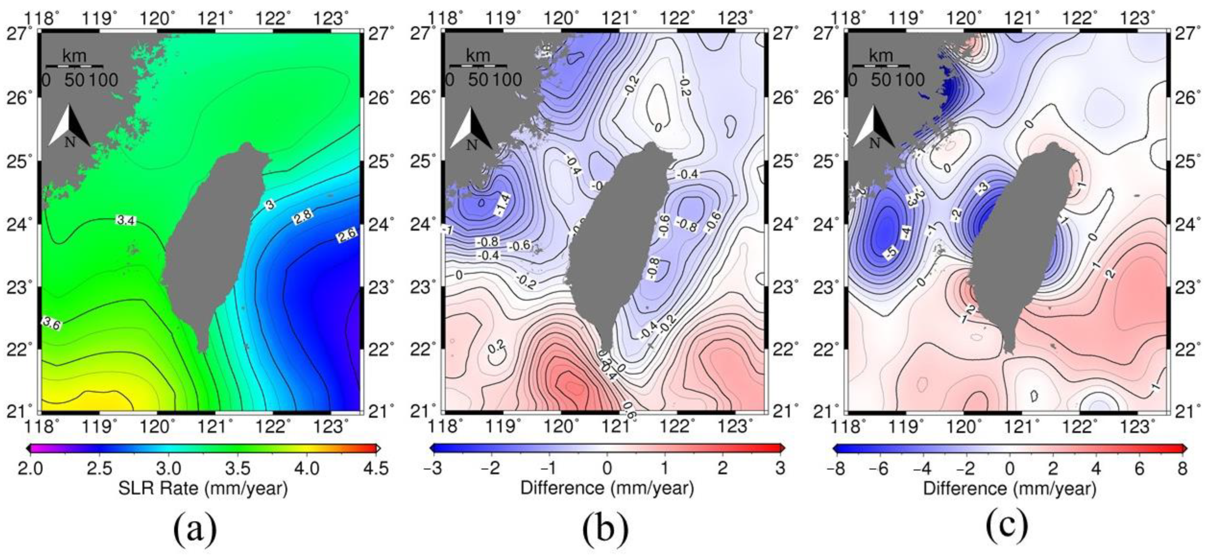
Using the along-track SLR rates determined in this study, we assessed the global SLR models, namely, NOAA, AVISO, and Yuan et al. (2021) [30], for their ability to provide accurate SLR rates in the waters near Taiwan. The NOAA model uses data from the T/P-Jason satellite series, including T/P, Jason-1, Jason-2, and J3, with a grid spacing of 30 min from epoch 1992.96 to 2021.92. Figure 2a shows the SLR rates near Taiwan from NOAA, which range from 2.0 to 4.0 mm/year. NOAA’s model shows that the largest SLR rates occur in the waters off southwest Taiwan. The SLR rates in the waters off Taiwan’s east coast are lower than 3.0 mm/year.
The AVISO model employs the L4 DAUC data from multiple satellite missions, including the T/P-Jason satellite series, CryoSat-2, and Sentinel-3. The differences between the SLR rates from NOAA and AVISO are shown in Figure 2b. The differences are irregular and range from −1.0 to 1.0 mm/year. In particular, the largest difference occurred in the Taiwan Strait and waters immediately off Taiwan’s east coast.
The third SLR model used for comparison was from Yuan et al. (2021), who utilized a method to divide all altimetry missions from 1993 to 2020 into nine groups and obtained nine mean sea surface models to calculate the SLR rates in each grid cell with a grid spacing of 1 min. Figure 2c shows the differences between the SLR rates from NOAA and Yuan et al. (2021), indicating substantial differences in the magnitude and spatial pattern compared with the NOAA–AVISO differences (Figure 2b). Again, irregular and larger differences occurred in the shallow waters around Taiwan.
The comparisons in Figure 2b,c highlight the challenges in obtaining accurate SLR rates in the waters around Taiwan, as is evident from the disparity in the SLR rates obtained by the three models. This suggests a need for continued efforts to refine SLR models around Taiwan by adding more high-quality altimeter and tide gauge data and using more sophisticated geophysical correction models for shallow waters.

2.3. The Mean Sea Surface Models and Global Geoid Model

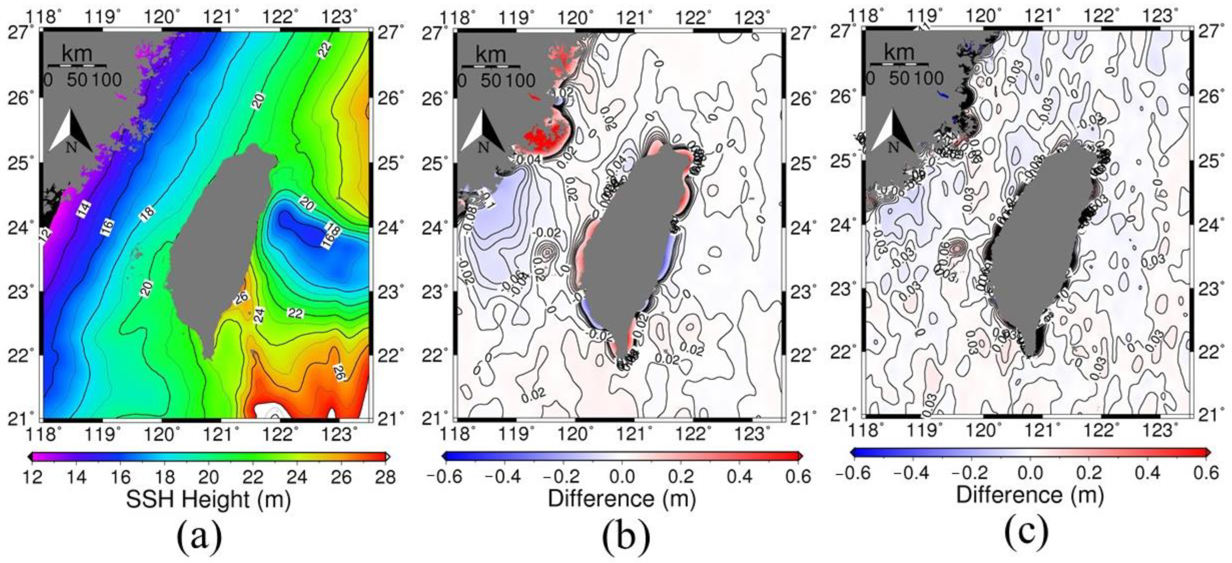
Three global MSS models were assessed in this study: CLS15, DTU18, and NCTUMS. The CLS15MSS model [19] was produced by CNES and is a continuation of the CLS2011 model, spanning latitudes from 80°S to 84°N. It was constructed using SSHs from multiple altimeter satellites at a rate of 1 Hz, with data obtained from 1993 to 2012. Specifically, the altimeter satellites used in constructing CLS15 include the missions of T/P, Jason-1, Jason-2, ERS-1, ERS-2, Envisat, GFO, and Cryosat-2. Figure 3a shows the SSHs from CLS15 near Taiwan. According to information from AVISO, the CLS15 model has made five breakthroughs compared with previous versions, namely, (1) significant improvements in short-wavelength signals, (2) better correction for ocean variability, (3) reduced deterioration of SLA in coastal areas, (4) significantly reduced errors in global SLA calculations, and (5) improved accuracy compared with previous versions.
The DTU18 MSS model [22], developed by the Technical University of Denmark (DTU), covers latitudes from 90°S to 90°N, and is different from the CLS15 model in that it uses different satellite data from those used by CLS15 and the data processing approaches of the two models are different. DTU18 also differs from its previous version, namely, DTU15, primarily in the recalculation of polar data, the correction of the T/P series satellite long-wave signals, and the inclusion of Sentinel-3A data near the coast. Figure 3b shows the differences between the SSHs from CLS15 and DTU18 near Taiwan.
The local MSS model of Taiwan, namely, NCTUMSS, was constructed for the use of a depth reference system for Taiwan. NCTUMSS is based on altimeter-derived mean SSHs, geoid undulations from the latest hybrid geoid model of Taiwan, and tide gauge data [12,31]. The altimeter data are from the missions T/P, Jason-1, Jason-2, J3, Envisat, SARAL, Cryosat-2, Sentinel-3, ICESat, and ICESat-2. The tide gauge data along the coast of Taiwan was provided by the Department of Geomatics at National Cheng Kung University. When constructing NCTUMSS, two important aspects were considered. First, because the accuracy of the altimeter data near the coast was lower, altimeter data within a certain distance (d) from the coast was not used. Second, discontinuities in the SSH at the ocean–land transition zone were minimized. We experimented with several possible combinations of the data sets, with d ranging from 5 to 15 km. Both Gaussian and median filters were applied to minimize the discontinuities at the transition zone. Our tests resulted in 18 MSS models around Taiwan. The best MSS model (NCTUMSS) was the one in which the differences between the SSHs from the 33 tide gauge stations and the modeled SSHs were the smallest. As a result, NCTUMSS excluded altimeter data within 5 km of the shorelines of Taiwan and the Gaussian filter was employed. Figure 3c shows the differences between the SSHs from CLS15 and NCTUMSS.
In Figure 3b,c, two consistent patterns can be observed. First, significant differences occurred in the coastal regions of Taiwan and mainland China. Second, there were substantial negative differences in the waters stretching from Penghu Island to the mainland China coast. Several factors may account for these patterns, including differences in altimeter data sets and the data-processing methods employed in the three models. Notably, NCTUMSS incorporated tide gauge measurements from around Taiwan while excluding altimeter data within 5 km of the coast, which could contribute to the differences observed in Figure 3c.
The global geoid model is computed from the Earth Gravitation Model 2008 (EGM08) [32] constructed by the US National Geospatial-Intelligence Agency (NGA). The EGM08 contains spherical harmonic coefficients up to degree and order 2160 and some coefficients of degrees higher than 2160. In this study, the EGM08-derived geoidal heights were used to reduce the SSHs from repeat cycles to the SSHs at the reference ground tracks (see Section 3).

3. Method for Determining Along-Track Sea Surface Heights and Their Rates of Change

3.1. Determining Satellite Reference Ground Tracks

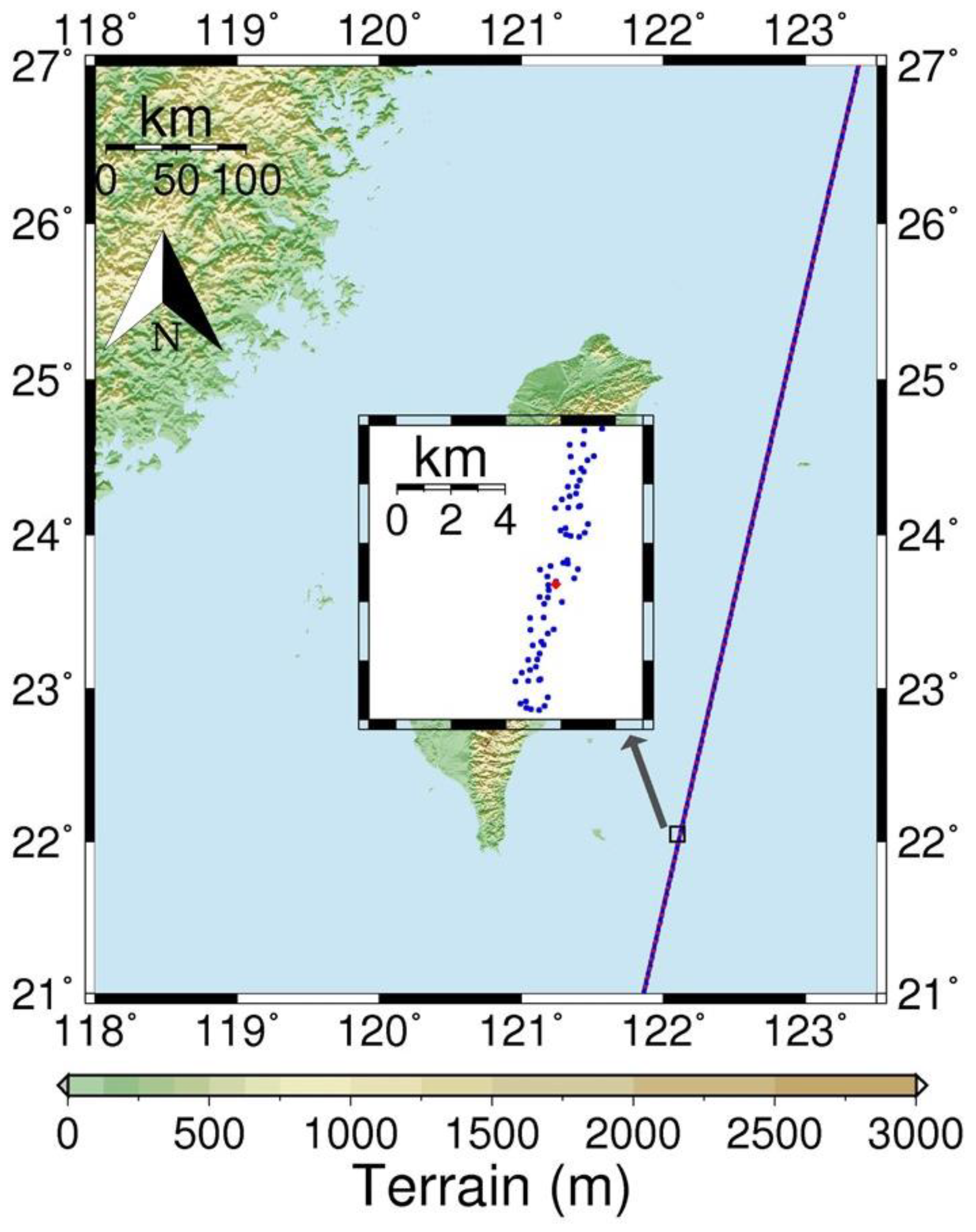
Upon acquiring L2P data from the AVISO ftp server and computing the sea surface ellipsoid heights using WGS84 as the reference ellipsoid, we classified the satellite data by orbit. For instance, S3B had 13 tracks with recorded data in the study area (Figure 1), while J3, T/P, and Jason series satellites had 5 tracks. However, it was not possible to compute MSS heights or SLR rates without observations taken at the same points along each of the tracks. To this end, we obtained a reference track for each of the S3B and J3 tracks by comparing the number of data points from all repeat cycles and then selecting the track with the most data points as the reference track. This is illustrated in Figure 4 for a reference track (pass 006) of S3B southeast of Taiwan. In Figure 4, the 1-HZ SSH observations are used. The red diamond represents a point along the reference track, and the blue points represent the points from the repeat cycles. The observed SSHs (all blue points) were reduced to the heights at the location of the red diamond (see Section 3.2). Our preliminary satellite processing automatically excluded anomalous data due to land effects, leading to varying numbers of data points for the same track for different cycles.

3.2. Reduction of Sea Surface Heights to the Reference Tracks

In this process, the recorded SSHs from successive cycles were reduced to the closest points on a reference track. The maximum permitted distance to the closest point was 5 km. The formula for the height reduction is expressed as
h = h E G M , r e f h E G M , p
h c o r = h p + h
where h E G M , r e f is the geoidal undulation from EGM08 at the reference track point, h E G M , p is the geoidal undulation at the non-reference track point, h p is the SSH measured from a repeat cycle at a non-reference track point, and h c o r is the reduced SSH. In this context, we assumed that the difference in ellipsoidal height is equivalent to the difference in geoidal undulation between a given observation point and its nearest reference point.

3.3. Outlier Detection

Upon the completion of the previous step, at each reference point, there will be a certain number of reduced SSHs and their observation times for determining the mean SSH and SLR at this point. However, outliers may exist in the reduced SSHs, which can distort the result. To remove outliers, the τ test at a given significance level was carried out. A reduced SSH forms the following observation equation:
h t   + v t = a + b t t 0 + c s i n 2 π t t 0 + d c o s 2 π t t 0 + e s i n 4 π t t 0 + f c o s 4 π t t 0
where h t   is the SSH; t 0 is the reference time; t is the time of observation (measured in seconds); and a, b, c, d, e, and f are the parameters to be estimated. Equation (3) describes the variations in SSH with time. The six parameters in Equation (3) are as follows: a is the mean SSH at the reference time; b is the SLR rate; and c, d, e, and f are the parameters that account for the annual and semi-annual SSH variations. The six parameters are determined by an iterative, least-squares method. For each iteration of the least-squares solution for the six parameters, the τ value of the residual of the kth observation (SSH) is computed as follows:
τ k = | v k |   σ ^ v k
where v k is the residual of the kth observation and σ ^ v k is the standard deviation of v k . Then, τ k   is compared against the critical tau value T defined by
T = τ 1 α n ; r , n q r = ( n q F α n ; r , n q r n q r + r F α n ; r , n q r ) 0.5
If τ k > T, the kth observation is likely an outlier. In Equation (5), n is the number of observations for each of the iterations, α is the significance level (set to 0.05 in this study), r is the number of possible outliers, q is the number of unknowns (six in this study), and F α n ; r , n q r is the critical F value with an α/n significance level and degrees of freedom of r and (n − q − r). The outlier detection was performed iteratively by removing one outlier in one iteration. The final least-squares solution for the six parameters is obtained from the outlier-free observations. The estimated a and b represent the mean SSH and SLR rate at t 0 , respectively, at the reference point. The solution also yields the standard deviations (error) of a and b, which represent the formal errors of a and b at the 68% confidence level (one-sigma errors).

3.4. Removing Nearshore Altimeter Data and Sample Time Series

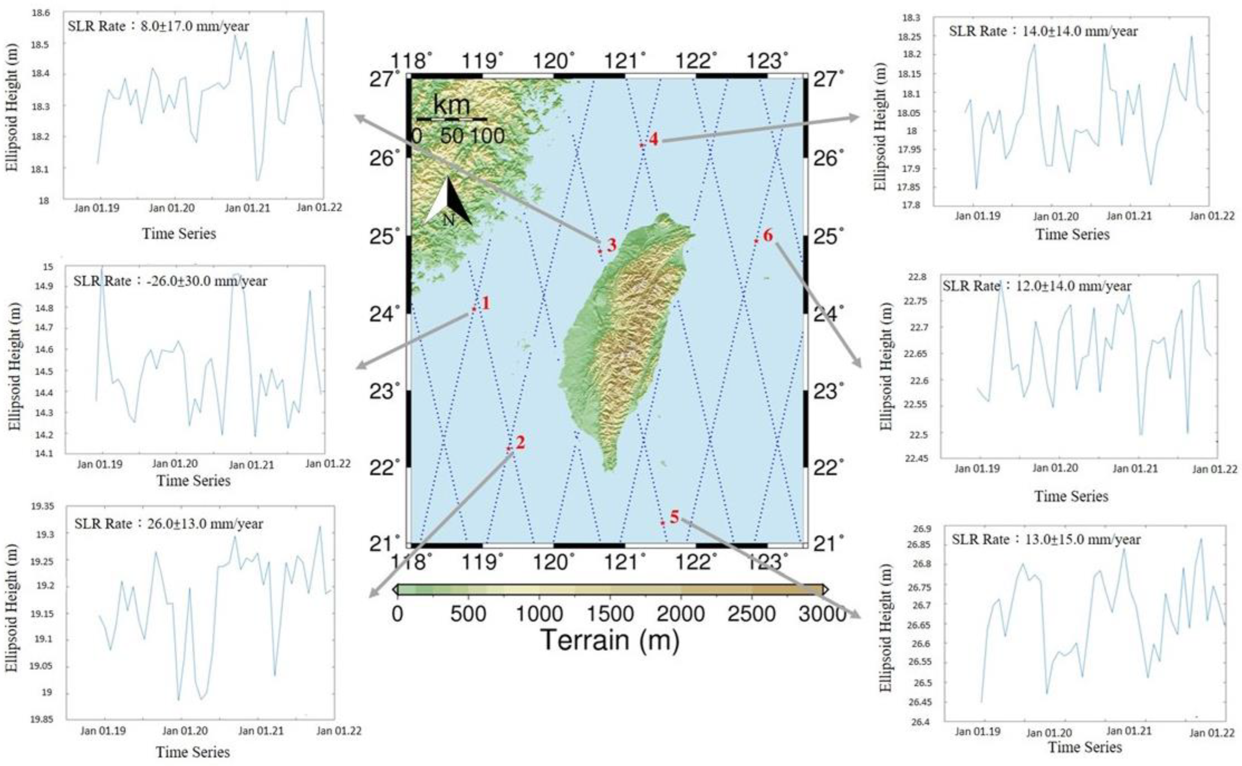
The original altimeter observations contained data points on land, which were removed within a 5 km range from the coastline using commands in the software Generic Mapping Tools (GMT; https://www.generic-mapping-tools.org accessed on 13 December 2021). Figure 5, Figure 6 and Figure 7 show the resulting reference tracks for the S3B, J3, and T/P-Jason satellite series near Taiwan after removing the coastal data. Note that the reference tracks displayed in Figure 6 and Figure 7 do not precisely align. The reason for this discrepancy is that the T/P-Jason satellite series covered a longer timeframe, ranging from 1992.96 to 2021.92, whereas the reference tracks for J3 encompassed only six years in this study. The reason for eliminating data points within this range was to adhere to the criteria used when constructing the NCTUMSS model, which excluded data within 5 km of the coast. By removing the data within this range, this study ensured that satellite data within 5 km of the coast was not used to determine along-track mean SSHs and SLR rates.
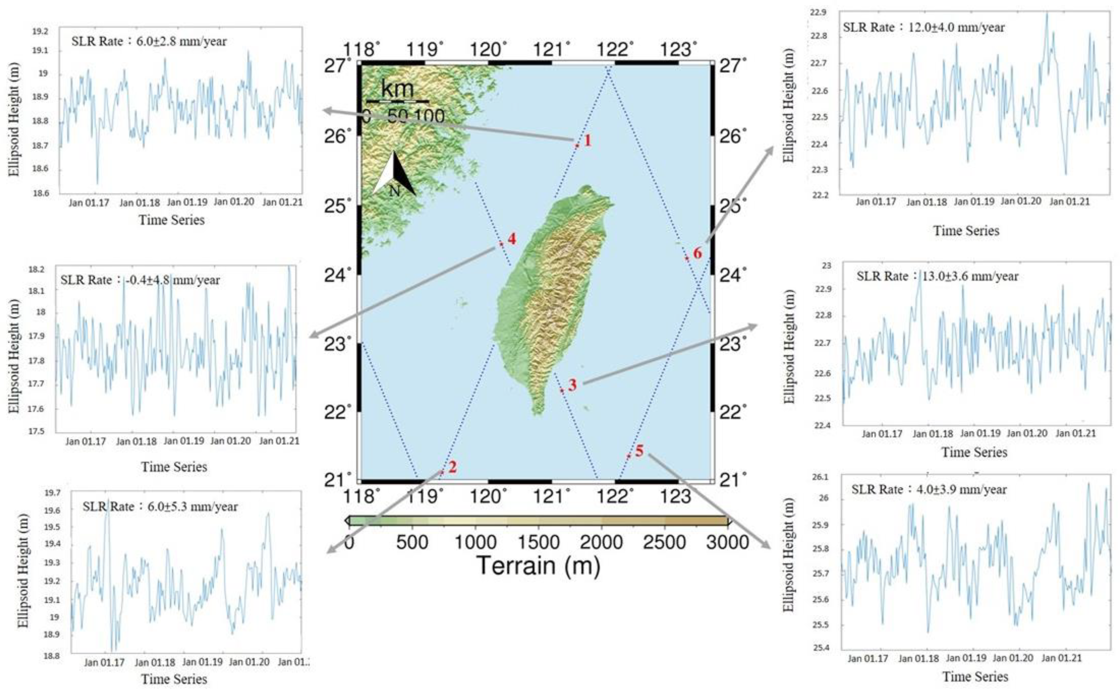
At each point along the reference track in Figure 5, Figure 6 and Figure 7, the reduced SSHs were used to create a time series of height changes without outliers (see Section 3.2). Six evenly distributed sample points (red dots in Figure 5, Figure 6 and Figure 7) were selected to demonstrate the time series. The time series and the SLR rates for the S3B, J3, and T/P-Jason satellite series are also shown in Figure 5, Figure 6 and Figure 7, respectively. With the exceptions of point 1 (Figure 5) in S3B and point 4 in J3 (Figure 6), the time series exhibited increasing trends in the SSH, accompanied by prominent seasonal oscillations. The characteristics of these oscillations varied depending on the location of the respective time series. The long-term time series from the T/P-Jason satellite series (Figure 7) resulted in stable SLR rates around Taiwan at about 3.0 mm/year, compared with the fluctuating SLR rates from the short-term S3B and J3 time series (Figure 5 and Figure 6).

4. Results and Discussion

4.1. The Along-Track SLR Rates: Impact of Data Quality

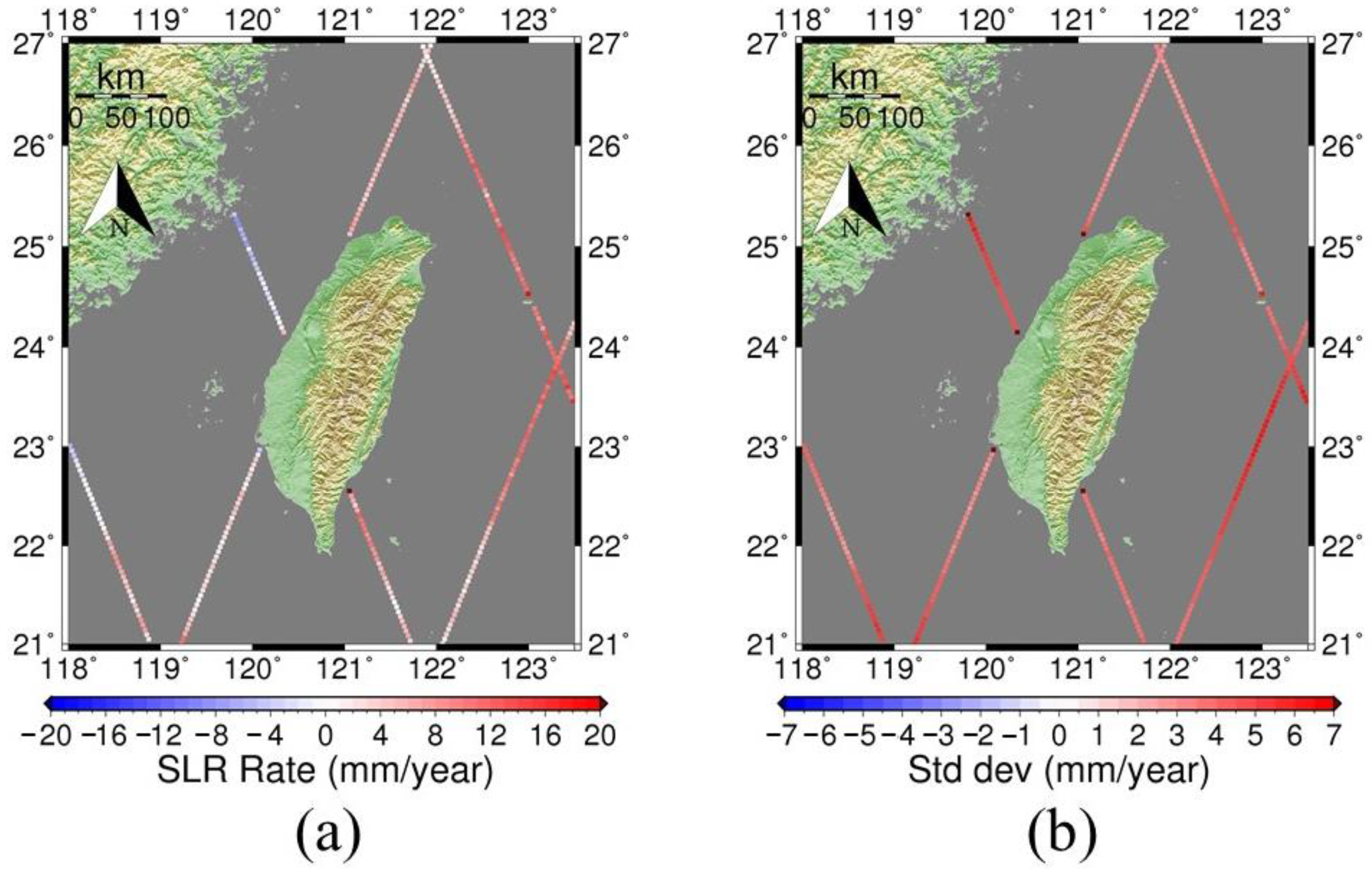
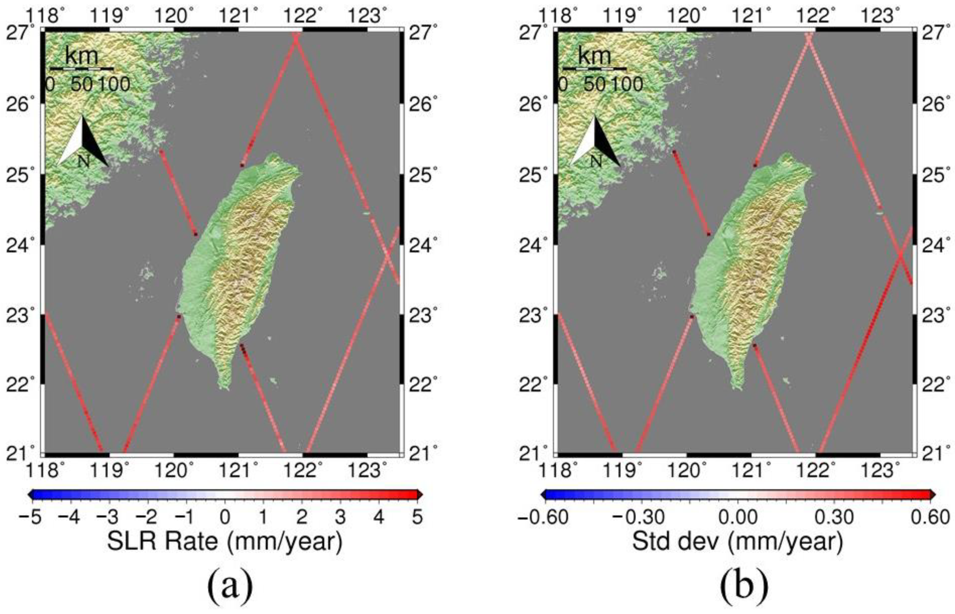
We used the method described in Section 3 to determine the SLR rates and their standard deviations from the outlier-free altimeter data along the reference tracks. Figure 8, Figure 9 and Figure 10 show the SLR rates and the standard deviations for S3B (three years), J3 (6 years), and the T/P-Jason satellite series (1992.96–2021.92). Table 1 shows the statistics of the along-track SLR rates from different missions and durations.
Figure 8a shows the SLR rates from S3B, which ranged from −85.6 to 73.2 mm/year, with an average of 6.6 mm/year. The regions with large SLR rates were in the southwestern waters of Taiwan and the Taiwan Strait near Penghu. Figure 9a shows the SLR rates from J3, which ranged from −8.4 to 20.3 mm/year, with an average of 5.5 mm/year. The areas with large rates were in the northeastern waters of Taiwan and the Taiwan Strait. The mean SLR rate from S3B was 6.6 mm/year and the mean from J3 was 5.5 mm/year (Table 1). These two mean rates were greater than the global mean of 3.0–3.3 mm/year.
Figure 10a shows the long-term SLR rates based on the data from the T/P-Jason satellite series spanning nearly three decades. The rates ranged from 1.8 to 5.7 mm/year, with an average of 3.2 mm/year, which is close to the global SLR rate. The SLR rates in the southeastern waters of Taiwan were relatively smaller than in other areas. This pattern was consistent with the pattern from the NOAA SLR model (Figure 2a). The results in Figure 8, Figure 9 and Figure 10 indicate that the SLR rates over different periods (short-term vs. long-term) and from different altimeter data sets were substantially different.
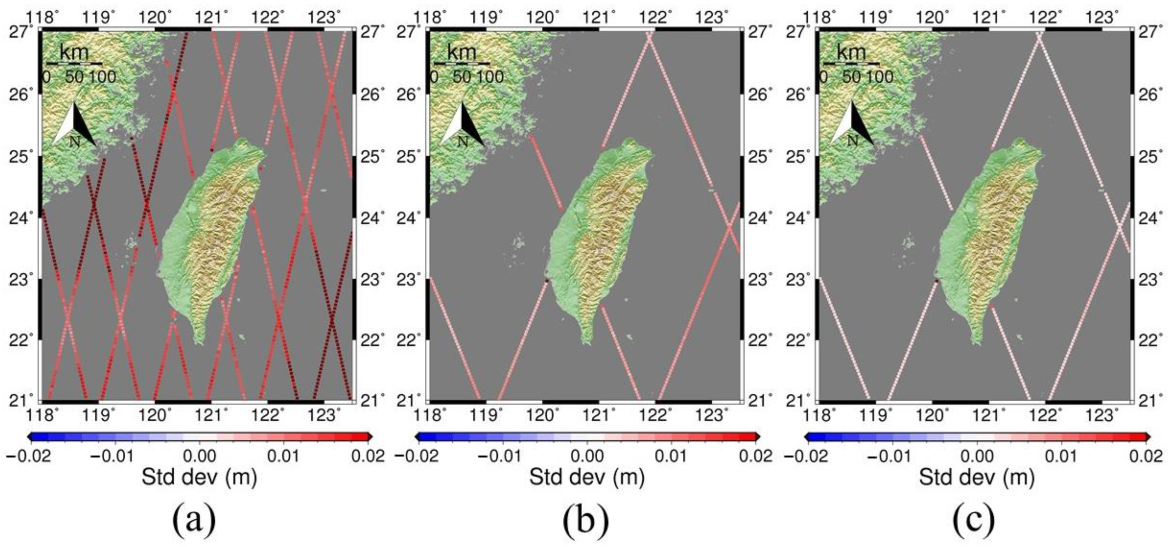
The standard deviations (errors) of the SLR rates from S3B ranged from 8.4 to 42.2 mm/year (Figure 8b), and those from J3 ranged from 2.6 to 12.4 mm/year (Figure 9b). This suggests that a longer time series could lead to a smaller standard deviation for an estimated SLR rate. The smallest standard deviations of SLR rates were from the long-term T/P-Jason satellite series and ranged from 0.2 to 0.8 mm/year (Figure 10b).
A greater uncertainty in the estimated SLR trend was indicated by a larger standard deviation. The spatial distributions of the standard deviations obtained from the three altimeter datasets in Figure 8b, Figure 9b and Figure 10b showed a strong similarity that was applicable to both the short- and long-term records. In general, the Taiwan Strait and the southeastern waters of Taiwan exhibited larger standard deviations. These larger standard deviations could be attributed to two factors. First, these regions may contain degraded altimeter data quality, particularly in the Taiwan Strait and immediate coastal areas. This quality degradation was primarily caused by inadequate tidal corrections and waveform contaminations, leading to substantial fluctuations in the measured sea surface heights (SSHs) from altimeters. Second, natural oceanic variations, such as the presence of the Kuroshio Current in the southeastern waters of Taiwan, could induce greater fluctuations in sea level.
The problem of degraded altimeter quality was further exemplified by the contrasting signs of the SLR rates near the crossover point where the ascending and descending tracks of S3B intersected, which was located northeast of Penghu (refer to Figure 8a). There are several potential factors that could explain these contrasting signs. First, the relatively shallow depth of the sea in the Taiwan Strait might cause secondary reflections of radar signals from the seafloor. Second, the accuracy of the ocean tide model used in the Taiwan Strait may not be sufficient to adequately correct for the effects of ocean tides. Third, variations in the functioning of the altimeter locking system during the ascending and descending passes could introduce biases in the measured ranges. Last, the presence of the landmass of Penghu near the crossover point could introduce contaminations to the altimeter waveforms, and the waveform re-tracking technique employed in this study may not effectively mitigate these contaminations.

4.2. The Short-Term SLR Rates and the Long-Term Rates: Differences and Cautions

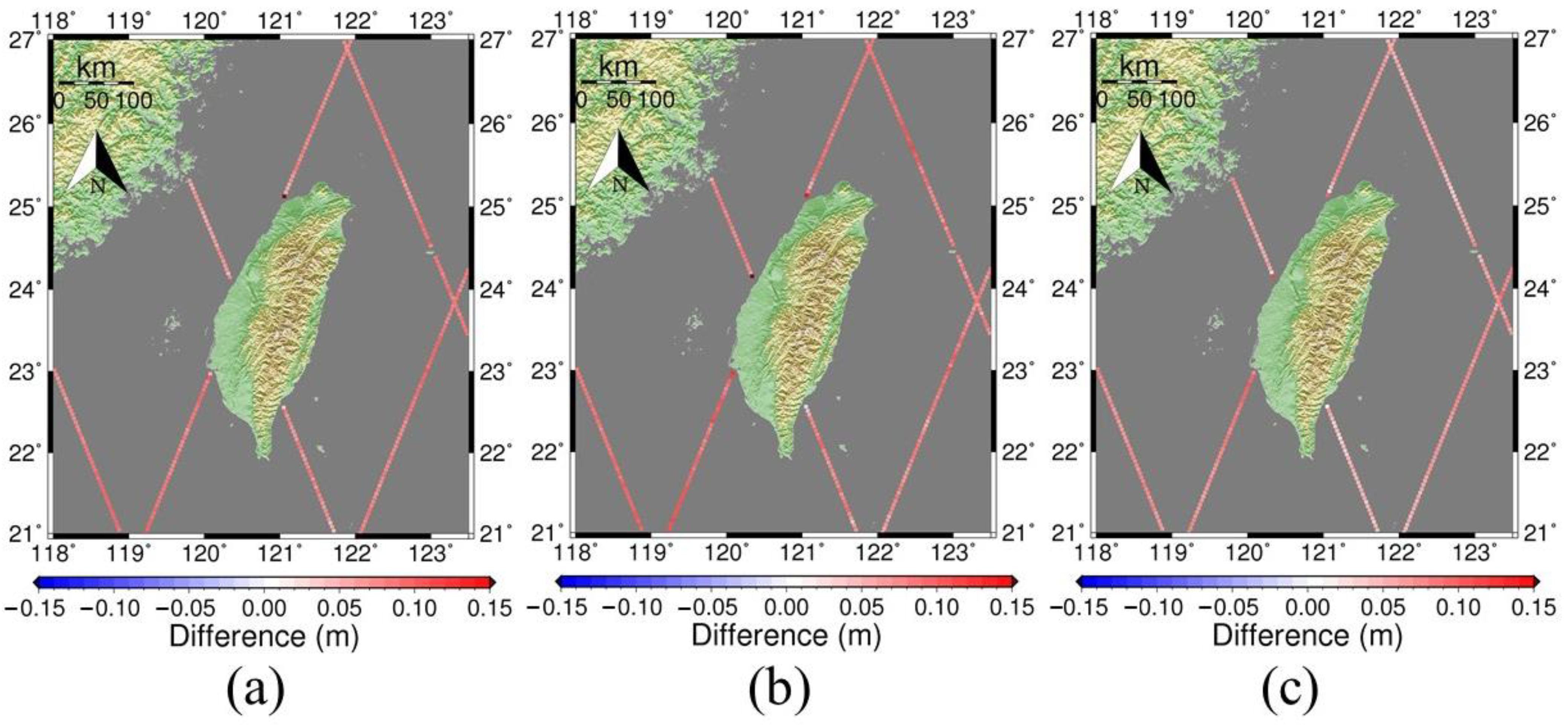
We conducted a comparison of the along-track SLR rates (Table 1 and Figure 8, Figure 9 and Figure 10), with the long-term SLR rates provided by NOAA and AVISO, as presented in Figure 3a,b, respectively. To facilitate the comparison, we first interpolated the SLR rates from NOAA and AVISO onto the reference tracks of S3B and J3. Next, we calculated the difference by subtracting these interpolated rates from the along-track SLR rates. The statistical analysis of these differences is presented in Table 2. The spatial distributions of the differences between S3B and NOAA, as well as S3B and AVISO, are illustrated in Figure 11a,b, respectively. Similarly, the differences for J3 are displayed in Figure 12a,b.
Based on our analysis results presented in Table 2 and Figure 11 and Figure 12, notable differences between the SLR rates derived from short-term altimeter records (S3B and J3, as documented in this study) and those obtained from long-term records (the global models of AVISO and NOAA) in the vicinity of Taiwan were identified. In terms of the spatial distribution, the discrepancies between S3B and the two global models (AVISO and NOAA) were most pronounced in Taiwan’s southwest offshore area and the Taiwan Strait. For J3, these disparities were more significant in Taiwan’s eastern waters and the Taiwan Strait.
The analysis using Table 2 and Figure 11 and Figure 12 has the following implications. When evaluating the impact of sea level rise using short-term data, it is important to note that while it may capture recent changes in sea level, its accuracy may be compromised. On the other hand, the long-term sea level record provides a more precise assessment but may not fully capture the most recent rates of sea level rise. Consequently, relying solely on the long-term trend for planning mitigation measures may not be entirely accurate when addressing the immediate impact of sea level rise. Therefore, a comprehensive approach that incorporates both short-term data for recent trends and long-term data for historical context is crucial in accurately assessing and planning for the consequences of sea level rise.

4.3. Accuracies of the MSS Models: Update Frequency

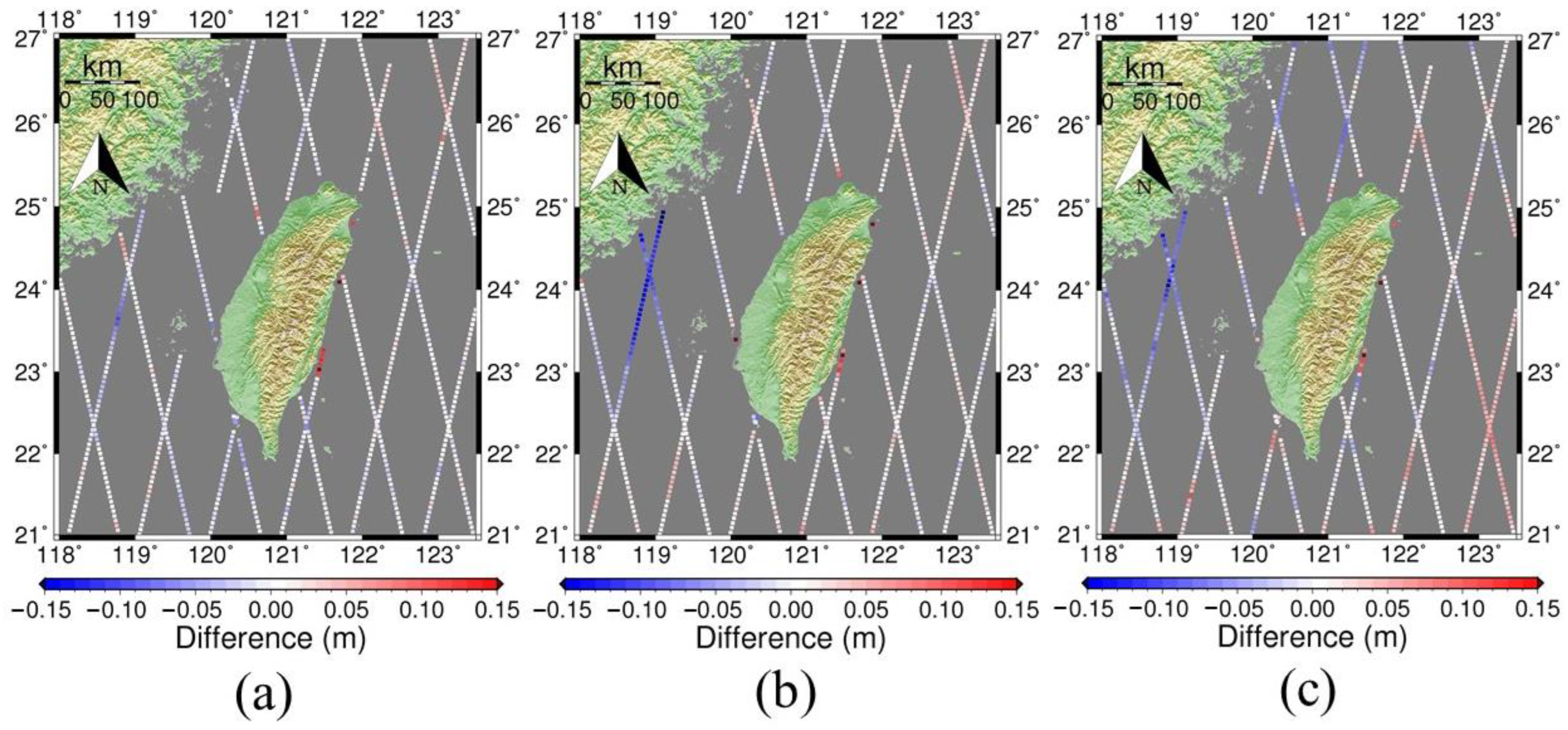
Here, we evaluate the differences between the along-track sea surface heights (SSHs) obtained from S3B and J3, and those derived from the CLS15, DTU18, and NCTUMSS5 MSS models. Similar to the comparison of SLR rates, we interpolated the SSHs from these three models onto the reference tracks of S3B and J3. Subsequently, we calculated the differences between the values obtained from S3B or J3 and the respective models. Table 3 shows the statistics of the differences. Figure 13 and Figure 14 show the spatial distributions of the differences.
The results presented in Table 3 and Figure 13 and Figure 14 indicate that there were no significant discrepancies between the mean sea surface heights (SSHs) derived from the CLS15, DTU18, and NCTUMSS models and those obtained from the along-track observations of S3B and J3. However, a consistent mean difference of approximately 8 cm was observed across all cases (Table 3, the mean difference column). This 8 cm mean difference arose due to the discrepancy in reference epochs between the models (1993) and the mean SSHs from S3B and J3 (2020.5 and 2019.0), respectively. Using this information, we inferred that the sea level rise (SLR) rates around Taiwan ranged from 3.0 to 3.2 mm/year, which aligned with the global mean SLR rate of approximately 3.0 mm/year. The differences in reference epochs between the various sources of MSS models highlight the importance of considering the reference epoch and the specific period during which measurements were collected when evaluating the accuracies of the models. This consideration is particularly crucial due to the current acceleration of sea level rise (SLR) rates, which can result in faster changes in the mean sea surface.
According to Table 3, the differences between the S3B MSS heights and the CLS15, DTU18, and NCTUMSS MSS heights along the reference tracks exhibited standard deviations in the range of 2–3 cm. The root-mean-square differences were approximately 8–9 cm, which could be attributed to the 8 cm mean differences presented in Table 3. For the J3 MSS heights, the standard deviations of the differences with the CLS15, DTU18, and NCTUMSS MSS along the tracks varied from 1.3 cm to 1.5 cm, with corresponding root-mean-square differences of about 8 cm, once again reflecting the 8 cm mean differences. Thus, in terms of the standard deviation, the SSHs derived from CLS15, DTU18, and NCTUMSS matched the along-track SSHs from S3B and J3 to within 2–3 cm. Figure 15 shows the standard deviations of the along-track mean SSHs obtained from the least-squares estimation using Equation (3).
Figure 13 shows significant differences between the along-track SSHs obtained from S3B and three models in the region spanning southeast mainland China and Penghu. In this region, DTU18 and NCTUMSS exhibited larger discrepancies compared with S3B, while CLS15 showed relatively smaller differences. These large differences could be attributed to the utilization of different geophysical correction models for S3B altimeter data and the data used in constructing the three models. Notable differences in Figure 13 also arose in immediate coastal areas due to inaccurate altimeter measurements near the coasts. In contrast, Figure 14 displays relatively uniform differences for J3, except in certain coastal areas. It is important to note that J3 does not traverse the mainland China-Penghu region, where significant differences existed for S3B, as shown in Figure 13.
Similar to the investigation of the SLR rates, we also examined the impact of data length on the standard deviations of SSHs around Taiwan by comparing the results from S3B and J3 to those from the T/P-Jason satellite series (Figure 15). The analysis indicated that longer data records led to smaller standard deviations, as expected. In general, the number of data points (n) and the data length were related to a reduction in standard deviation by a factor of 1 / n (as shown in Figure 15a,c), which aligned with the error propagation theory. Larger standard deviations of SSHs were found in the Taiwan Strait and southeastern coastal regions of Taiwan, indicating greater fluctuations in the altimeter-measured SSHs, either due to data noises, poor geophysical corrections, or changing sea states, or all of them. Furthermore, the standard deviations of SSHs obtained from S3B, J3, and the TOPEX-Jason series were on the order of cm or even mm, suggesting that the use of along-track SSHs is suitable for verifying mean sea surface models around Taiwan at mm–cm levels.
The determination of the update frequency for a mean sea surface model involves considering various global models of sea level rise rate factors, such as the specific application requirements, data availability, temporal variability of the sea surface, and desired accuracy. The appropriate update frequency can range from months to years, depending on these factors. Regular assessment and evaluation of the model’s performance, as well as comparisons with new data, are crucial in determining the optimal update frequency. For example, when assessing the performance of NCTUMSS using S3B and J3 data (Table 3), the mean accuracy was found to be (0.0313 + 0.0140)/2 = 0.0226 cm for NCTUMSS. Assuming an average SLR rate of 0.0033 m/year (Table 1, T/P series), the estimated update frequency would be approximately 0.0226/0.0033, which is approximately 7 years.

5. Conclusions

This study assessed the accuracies of commonly used mean sea surface models and a local model by analyzing the latest S3B and J3 altimeter data along their respective tracks. Our findings indicate that the SLR rates around Taiwan exhibited spatial variations and that the rates derived from global models, as well as S3B and J3, had limitations in terms of their spatial resolution and accuracy. The observed higher SLR rates in the past 3–6 years compared with the long-term rates suggested a potentially increasing influence of climate change on the sea level. Factors such as shallow water depths in the Taiwan Strait and the presence of the Penghu landmass, along with rapidly changing sea states, contributed to relatively large errors in the altimetry measurements.
Among the MSS models examined, CLS15 demonstrated the highest accuracy. The NCTUMSS and DTU18 models exhibited differences in the spatial distribution of the SSH, which were likely due to unsuppressed high-frequency noises and errors in geophysical corrections. The most important feature of NCTUMSS is that this model combines multiple-altimeter mission data, Taiwan’s tide gauge measurements, and Taiwan’s hybrid geoid for a smooth transition from ocean to land. Thus, NCTUMSS is suitable for constructing a depth datum around Taiwan.
A key takeaway from this study is that effectively evaluating and preparing for the consequences of rising sea levels requires a comprehensive approach. This approach should recognize the constraints of short-term data, which may only reflect recent changes without complete accuracy, as well as the more precise but potentially outdated long-term sea level record, which might not capture the current accelerated rates of sea level rise.

Author Contributions

C.H. was the PI of the projects leading to this paper. Y.-S.H., C.H. and T.-W.C. wrote the manuscript, and Y.-H.C. helped with the computations and editing. All authors have read and agreed to the published version of the manuscript.

Funding

This research was supported by grants from the National Science and Technology Council of Taiwan under grants 109-2221-E-009-015-MY3 and 111-2611-M-A49-001. This study was partially supported by the Ministry of the Interior, Taiwan, under grant no. 112PA005.

Data Availability Statement

The time series of along-track SSHs and SLR rates determined in this paper, the MSS model NCTUMSS, and the materials in [12] can be retrieved from the ftp site: http://space.cv.nctu.edu.tw/publications/#data, accessed on 13 December 2021. The MSSH model DTU18 was from the authors of [22], the SLR model of [30] was from the authors, and the MSS model CLS15 is accessible from the ftp site: https://www.aviso.altimetry.fr/en/my-aviso-plus.html, accessed on 13 December 2021.

Conflicts of Interest

The authors declare no conflict of interest.

References

  1. Nicholls, R.J.; Cazenave, A. Sea-level rise and its impact on coastal zones. Science 2010, 328, 1517–1520. [Google Scholar] [CrossRef] [PubMed]
  2. Nicholls, R.J.; Marinova, N.; Lowe, J.A.; Brown, S.; Vellinga, P.; de Gusmao, D.; Hinkel, J.; Tol, R.S.J. Sea-level rise and its possible impacts given a beyond 4 C world in the twenty-first century. Philos. Trans. R. Soc. A 2011, 369, 161–181. [Google Scholar] [CrossRef] [PubMed] [Green Version]
  3. Cazenave, A.; Dieng, H.B.; Meyssignac, B.; Schuckmann, K.V.; Decharme, B.; Berthier, E. The rate of sea-level rise. Nat. Clim. Chang. 2014, 4, 358–361. [Google Scholar] [CrossRef]
  4. Niu, Y.; Guo, J.; Yuan, J.; Zhu, C.; Zhou, M.; Liu, X.; Ji, B. Prediction of sea level change in Japanese coast using singular spectrum analysis and autoregression moving average. Chin. J. Geophys. 2020, 63, 3263–3274. [Google Scholar]
  5. Voosen, P. Seas are rising faster than ever. Science 2020, 370, 901. [Google Scholar] [CrossRef]
  6. Cazenave, A.; Llovel, W. Contemporary SLR. Annu. Rev. Mar. Sci. 2010, 2, 145–173. [Google Scholar] [CrossRef] [Green Version]
  7. Guo, J.; Wang, J.; Hu, Z.; Hwang, C.; Chen, C.; Gao, Y. Temporal-spatial variations of sea-level over China seas derived from altimeter data of TOPEX/Poseidon, Jason-1 and Jason-2 from 1993 to 2012. Chin. J. Geophys. 2015, 58, 3103–3120. [Google Scholar]
  8. Mu, D.; Yan, H. The instantaneous rate of global mean sea-level rise. Chin. J. Geophys. 2018, 61, 4758–4766. [Google Scholar]
  9. Tseng, Y.H.; Breaker, L.C.; Chang, E.T.Y. Sea level variations in the regional seas around Taiwan. J. Oceanogr. 2010, 66, 27–39. [Google Scholar] [CrossRef]
  10. Lan, W.H.; Kuo, C.Y.; Kao, H.C.; Lin, L.C.; Shum, C.K.; Tseng, K.H.; Chang, J.C. Impact of geophysical and datum corrections on absolute sea-level trends from tide gauges around Taiwan, 1993–2015. Water 2017, 9, 480. [Google Scholar] [CrossRef] [Green Version]
  11. Hung, W.C.; Hwang, C.; Chen, Y.A.; Zhang, L.; Chen, K.H.; Wei, S.H.; Lin, S.H. Land subsidence in Chiayi, Taiwan, from compaction well, leveling and alos/palsar: Aquaculture-induced relative SLR. Remote Sens. 2017, 10, 40. [Google Scholar] [CrossRef] [Green Version]
  12. Hwang, C. Depth modernization. Presented at the Taiwan Geosciences Assembly, Taipei, Taiwan, 7–10 June 2022. Available online: http://www.cgu.org.tw/index.php/2022-taiwan-geosciences-assembly-tga (accessed on 27 September 2021).
  13. Andersen, O.B.; Knudsen, P. DNSC08 mean sea surface and mean dynamic topography models. J. Geophys. Res. Ocean. 2009, 114, 327–432. [Google Scholar] [CrossRef]
  14. Marsh, J.G.; Koblinsky, C.J.; Zwally, H.J.; Brenner, A.C.; Beckley, B.D. A global mean sea surface based upon GEOS 3 and Seasat altimeter data. J. Geophys. Res. 1992, 97, 4915–4921. [Google Scholar] [CrossRef]
  15. Yuan, J.; Guo, J.; Niu, Y.; Zhu, C.; Li, Z. Mean Sea Surface Model over the Sea of Japan Determined from Multi-Satellite Altimeter Data and Tide Gauge Records. Remote Sens. 2020, 12, 4168. [Google Scholar] [CrossRef]
  16. Hernandez, F.; Schaeffer, P. The CLS01 Mean Sea Surface: A Validation with the GSFC00.1 Surface; CLS: Ramonville St Agne, France, 2001. [Google Scholar]
  17. Schaeffer, P.; Ollivier, A.; Faugere, Y.; Bronner, E.; Picot, N. The new CNES CLS 2010 mean sea surface. In Proceedings of the Oral Presentation at OSTST Meeting, Lisbon, Portugal, 18–22 October 2010; pp. 21–22. [Google Scholar]
  18. Schaeffer, P.; Faug’ere, Y.; Legeais, J.F.; Ollivier, A.; Guinle, T.; Picot, N. The CNES_CLS11 Global Mean Sea Surface Computed from 16 Years of Satellite Altimeter Data. Mar. Geod. 2012, 35 (Suppl. 1), 3–19. [Google Scholar] [CrossRef]
  19. Pujol, M.I.; Schaeffer, P.; Faugère, Y.; Raynal, M.; Dibarboure, G.; Picot, N. Gauging the improvement of recent mean sea surface models: A new approach for identifying and quantifying their errors. J. Geophys. Res. Ocean. 2018, 123, 5889–5911. [Google Scholar] [CrossRef]
  20. Andersen, O.B.; Knudsen, P.; Stenseng, L. The DTU13 MSS (mean sea surface) and MDT (mean dynamic topography) from 20 years of satellite altimetry. In Proceedings of the 3rd International Gravity Field Service (IGFS), Shanghai, China, 30 June–6 July 2014; Jin, S., Barzaghi, R., Eds.; Springer: Cham, Switzerland, 2015; Volume 144, pp. 111–121. [Google Scholar]
  21. Andersen, O.B.; Piccioni, G.; Stenseng, L.; Knudsen, P. The DTU15 MSS (mean sea surface) and DTU15LAT (lowest astronomical tide) reference surface. In Proceedings of the ESA Living Planet Symposium 2016, Prague, Czech Republic, 9–13 May 2016. [Google Scholar]
  22. Andersen, O.B.; Knudsen, P.; Stenseng, L. A new DTU18 MSS mean sea surface improvement from SAR altimetry. In Proceedings of the 25 Years of Progress in Radar Altimetry Symposium, Ponta Delgada, Portugal, 24–29 September 2018. [Google Scholar]
  23. Jiang, W.; Li, J.; Wang, Z. Determination of global mean sea surface WHU2000 using multi-satellite altimetric data. Chin. Sci. Bull. 2002, 47, 1664–1668. [Google Scholar] [CrossRef]
  24. Jin, T.Y.; Li, J.C.; Jiang, W.P.; Wang, Z.T. The new generation of global mean sea surface height model based on multi-altimetric data. Acta Geod. Cartogr. Sin. 2011, 40, 723–729. [Google Scholar]
  25. Jin, T.Y.; Li, J.C.; Jiang, W.P. The global mean sea surface model WHU2013. Geod. Geodynamics 2016, 7, 202–209. [Google Scholar] [CrossRef] [Green Version]
  26. Parisot, F.; Wilson, S. EUMETSAT and NOAA—The Jason-2 follow-on issue. In Proceedings of the 2008 OSTST (Ocean Surface Topography Science Team Meeting) Meeting, Nice, France, 10–15 November 2008. [Google Scholar]
  27. Parisot, F. EUMETSAT Altimetry programs. In Proceedings of the OSTST (Ocean Surface Topography Science Team) 2009 meeting, Seattle WA, USA, 22–24 June 2009. [Google Scholar]
  28. Bannoura, W.; Parisot, F.; Vaze, P.; Zaouche, G. J3 Project Status. In Proceedings of the OSTST (Ocean Surface Topography Science Team) 2012 Meeting Presentations, Venice, Italy, 27–29 September 2012. [Google Scholar]
  29. Barnoud, A.; Picard, B.; Meyssignac, B.; Marti, F.; Ablain, M.; Roca, R. Reducing the uncertainty in the satellite altimetry estimates of global mean sea level trends using highly stable water vapour climate data records. J. Geophys. Res. Ocean. 2023, 128, e2022JC019378. [Google Scholar] [CrossRef]
  30. Yuan, J.; Guo, J.; Zhu, C.; Hwang, C.; Yu, D.; Sun, M.; Mu, D. High-resolution sea level change around China seas revealed through multi-satellite altimeter data. Int. J. Appl. Earth Obs. Geoinf. 2021, 102, 102433. [Google Scholar] [CrossRef]
  31. Chen, T.W. Examining SLR and Mean Sea Surface Models around Taiwan Using Latest Satellite Altimetry Data from S3B and J3. Master’s Thesis, National Yang Ming Chiao Tung University, Hsinchu, Taiwan, 2022. [Google Scholar]
  32. Pavlis, N.K.; Holmes, S.A.; Kenyon, S.C.; Factor, J.K. The development and evaluation of the Earth Gravitational Model 2008 (EGM2008). J. Geophys. Res. Solid Earth 2012, 117, B04406. [Google Scholar] [CrossRef] [Green Version]
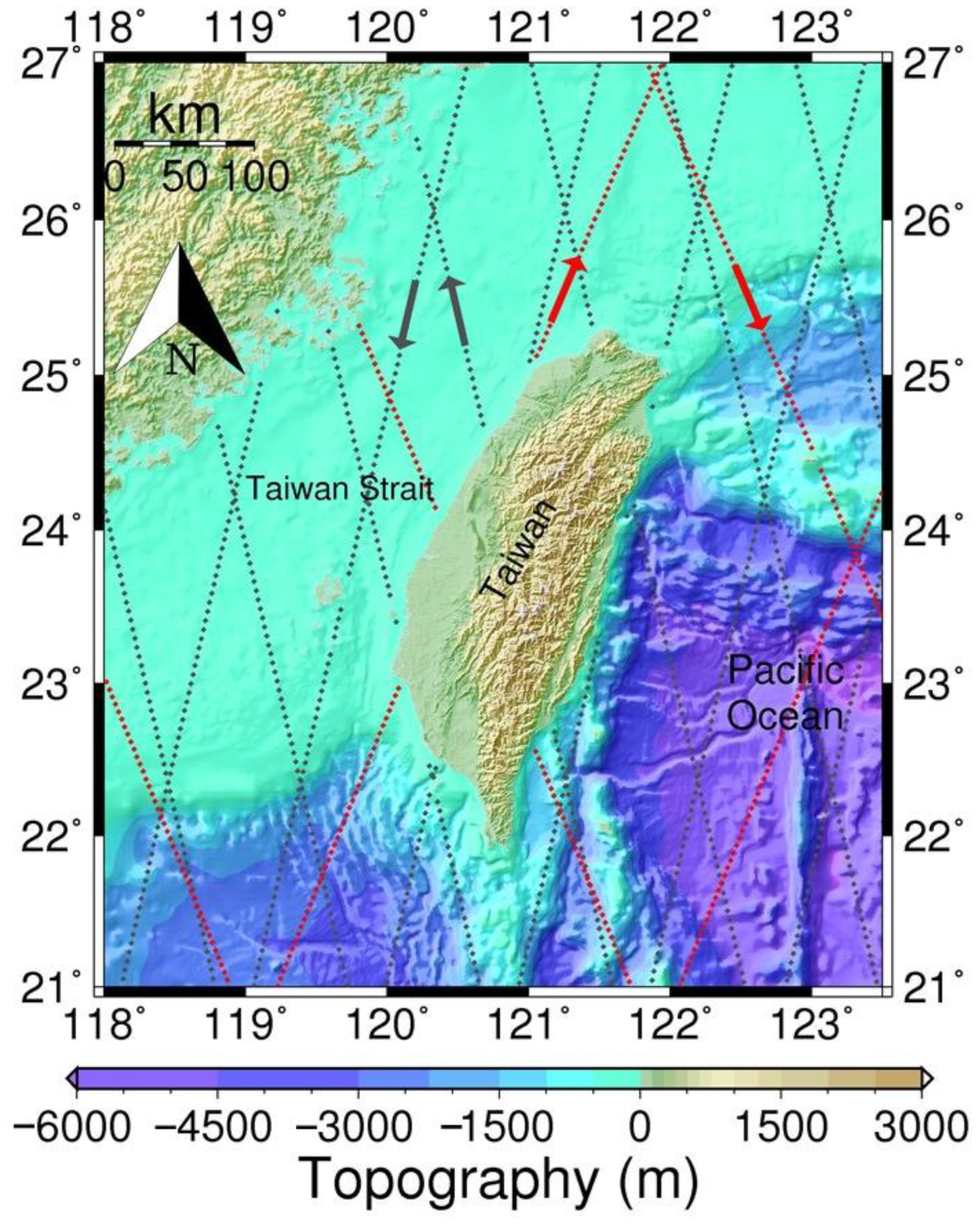
Figure 1. Elevations and depths around Taiwan. The red and gray dashed lines represent the reference tracks of the S3B and J3 missions, respectively. The arrows show the directions of satellite motions.
Remotesensing 15 03640 g001
Figure 2. (a) The SLR rates (unit: mm/year) derived from the NOAA model, (b) the differences between the SLR rates from NOAA and AVISO, and (c) the differences between the SLR rates from NOAA and Yuan et al. (2021).
Remotesensing 15 03640 g002
Figure 3. (a) The mean sea surface (ellipsoidal) heights of CLS15, (b) the differences between the SSHs from CLS15 and DTU18, and (c) the differences between the SSHs from CLS15 and NCTUMSS.
Remotesensing 15 03640 g003
Figure 4. A sample spot off southeast Taiwan showing the locations of along-track SSH observations from repeat cycles (blue dots) and the location of a point along the reference track (red diamond) of pass 006 of S3B.
Remotesensing 15 03640 g004
Figure 5. The reference ground tracks (blue dots) of S3B, and the SSH time series at the 6 sample points (red dots).
Remotesensing 15 03640 g005
Figure 6. The reference ground tracks (blue dots) of J3, and the SSH time series at the 6 sample points (red dots).
Remotesensing 15 03640 g006
Figure 7. The reference ground tracks (blue dots) of T/P, and the SSH time series at the 6 sampling points (red dots).
Remotesensing 15 03640 g007
Figure 8. (a) The SLR rates and (b) their standard deviations (errors, Section 3.4) along the S3B reference tracks. The time series for the S3B in this study was from November 2018 to December 2021.
Remotesensing 15 03640 g008
Figure 9. (a) The SLR rates and (b) their standard deviations (errors) along the J3 reference tracks. The time series for the J3 in this study was from February 2016 to December 2021.
Remotesensing 15 03640 g009
Figure 10. (a) The SLR rates and (b) their standard deviations (errors) along the T/P-Jason satellite series reference tracks. The time series for the T/P-Jason satellite series in this study was from December 1992 to December 2021.
Remotesensing 15 03640 g010
Figure 11. The differences between the short-term SLR rates from S3B and from (a) NOAA and (b) AVISO. The time series for the S3B in this study was from November 2018 to December 2021.
Remotesensing 15 03640 g011
Figure 12. The differences between the short-term SLR rates from J3 and from (a) NOAA and (b) AVISO. The time series for the J3 in this study was from February 2016 to December 2021.
Remotesensing 15 03640 g012
Figure 13. The differences between the along-track SSHs from S3B and from (a) CLS15, (b) DTU18 and (c) NCTUMSS. The time series for the S3B in this study was from November 2018 to December 2021.
Remotesensing 15 03640 g013
Figure 14. The differences between the along-track SSHs from J3 and from (a) CLS15, (b) DTU18, and (c) NCTUMSS. The time series for the J3 in this study was from February 2016 to December 2021.
Remotesensing 15 03640 g014
Figure 15. The standard deviations of the along-track mean surface heights from (a) S3B, (b) J3, and (c) T/P-Jason satellite series (unit: m). The time series for the S3B, J3, and T/P-Jason satellite series in this study were from November 2018 to December 2021, February 2016 to December 2021, and December 1992 to December 2021, respectively.
Remotesensing 15 03640 g015
Table 1. Statistics of the along-track SLR rates from different missions and durations (unit: mm/year).
MissionDuration
(Years)
MeanMax.Min.Std. Dev.
S3B36.673.2−85.619.3
J365.520.3−8.45.0
T/P series293.35.71.80.5
Table 2. Statistics of the differences in the SLR rates between S3B and NOAA, S3B and AVISO, J3 and NOAA, and J3 and AVISO (unit: mm/year).
MeanMaxMinStd. Dev.RMS
S3B–NOAA3.469.2−88.819.419.6
S3B–AVISO3.369.6−89.319.619.9
J3–NOAA2.217.2−11.65.25.6
J3–AVISO2.416.8−12.15.15.6
Table 3. Statistics of the differences between the along-track SSHs from S3B and J3 and those from CLS1, DTU18, and NCTUMSS (unit: m).
MeanMax.Min.Std. Dev.RMS
S3B-CLS150.08400.1816−0.01780.02060.0865
S3B-DTU180.08130.1800−0.10170.03530.0886
S3B-NCTUMSS0.08430.2059−0.03540.03130.0899
J3-CLS150.07750.18270.02060.01320.0786
J3-DTU180.08230.1580−0.01760.01500.0836
J3-NCTUMSS0.08220.13870.02480.01400.0834
Disclaimer/Publisher’s Note: The statements, opinions and data contained in all publications are solely those of the individual author(s) and contributor(s) and not of MDPI and/or the editor(s). MDPI and/or the editor(s) disclaim responsibility for any injury to people or property resulting from any ideas, methods, instructions or products referred to in the content.