Article

Spatiotemporal Variations of Global Human-Perceived Heatwave Risks and their Driving Factors Based on Machine Learning

1
State Key Laboratory of Resources and Environmental Information System, Institute of Geographic Sciences and Natural Resources Research, Chinese Academy of Sciences, Beijing 100101, China
2
College of Resources and Environment, University of Chinese Academy of Sciences, Beijing 101408, China
3
Jiangsu Center for Collaborative Innovation in Geographic Information Resource Development and Application, Nanjing 210023, China
*
Author to whom correspondence should be addressed.
Remote Sens. 2023, 15(14), 3627; https://doi.org/10.3390/rs15143627
Submission received: 10 June 2023 / Revised: 11 July 2023 / Accepted: 18 July 2023 / Published: 21 July 2023

Abstract

:
With ongoing global warming, heatwave-related disasters are on the rise, exerting a multifaceted impact on both the natural ecosystem and human society. While temperature has been extensively studied in the effects of extreme heat on human health, humidity has often been ignored. It is crucial to consider the combined influence of temperature and humidity when assessing heatwave risks and safeguarding human well-being. This study, leveraging remote sensing products and reanalysis data, presented the first analysis of the spatiotemporal variations in global human-perceived heatwaves on a seasonal scale from 2000 to 2020, and further employed the Random Forest (RF) regression model to quantitatively assess the explanatory power of seven driving factors. The study found that since the 21st century (1) changes in Heat Index (HI) have varied significantly worldwide, with the majority of regions witnessing an increase, particularly at higher latitudes. The largest HI-increasing area was observed in the second quarter (S2), while the overall HI increase peaked in the third quarter (S3); (2) except for the decreasing area of none-risk regions, the regions under all other risk levels expanded (the proportion of high-risk areas in the world increased from 2.97% to 3.69% in S2, and from 0.04% to 0.35% in the fourth quarter (S4)); (3) aspect demonstrated the greatest explanatory power for the global heatwave distribution (0.69–0.76), followed by land-use coverage (LUCC, 0.48–0.55) and precipitation (0.16–0.43), while the explanatory power of slope and nighttime light (NTL) was rather low; (4) over the years, the explanatory power of each factor for heatwave distribution underwent a minor decrease without significant trend, but exhibited seasonal periodicity. Climatic factors and LUCC were most impactful in the first quarter (S1), while DEM and other human factors dominated in S2; and (5) interaction factors showed no significant trends over the years, but the explanatory power of DEM and slope increased notably when interacting with climate factor, aspect, and LUCC, respectively. The interactions between the aspect and LUCC with precipitation yielded the highest explanatory power (above 0.85) across all interactions. To effectively tackle heatwave risks, it is suggested to concentrate on high-latitude regions, reinforce land use and urban planning with eco-friendly strategies, scrutinize the interplay between precipitation and heatwaves, capitalize on topographic data for devising well-informed prevention measures, and tailor response strategies to accommodate seasonal fluctuations. This study offers valuable insights for enhancing climate change adaptation, disaster prevention, and mitigation strategies, ultimately contributing to the alleviation of extreme heatwaves and risk reduction.

1. Introduction

Heatwaves have profound impacts on various aspects of human activities and natural ecosystems, such as threatening human health [1], increasing morbidity [2] and mortality [3], reducing worker productivity [4], damaging public facilities, and reducing crop yields [5] and economic output [6]. In the current global warming environment, scholars have observed a significant increase in heatwaves in several regions [7,8,9,10], jeopardizing rapid and sustainable global development [11,12,13,14]. Many experts in the field of climate change are currently conducting studies on extreme heat and its risk, most of which have traditionally focused only on the most fundamental single variable, i.e., near-surface temperature. However, the complex nature of these events necessitates a more comprehensive understanding beyond temperature alone.
To better understand extreme heat events and their effects, scholars are increasingly working on the interaction between temperature and other factors [15,16,17,18,19,20]. In hot environments, the human body relies on perspiration to dissipate heat and maintain its well-being, and high relative humidity can impede the body’s convection and heat dissipation abilities. In severe cases, the inability to effectively dissipate heat can lead to elevated body temperatures beyond the body’s tolerance, resulting in various heat-related illnesses and even fatalities. Therefore, focusing solely on near-surface air temperature is insufficient to accurately assess the comfort level of the environment for human health [20,21], and it is crucial to consider the synergistic effects of temperature and humidity when studying heatwave risks, which are at the forefront of current climate change prediction research [22,23,24,25,26,27]. However, studies in relation to heat events that consider the synergistic effects of temperature and humidity which are more reflective of real human comfort remain limited. As a result, these studies lack sufficient reference value for fully understanding the actual impact on human beings. Besides, further research is also needed to better understand the main influencing factors and driving mechanisms involved.
Previous qualitative analyses in spatiotemporal variability of extreme heat events and their attribution have mostly relied on methods such as linear regression [28,29,30], which are important for understanding the drivers of extreme heat variability, but may also lack a certain degree of objectivity in the analysis. In contrast, RF regression offers several advantages over traditional methods [31]. By utilizing multiple decision trees, RF regression can capture complex nonlinear relationships, allowing for the learning of diverse patterns and features in the data. Additionally, RF regression is robust against noise and outliers, as it averages predictions from multiple trees, thus reducing the impact of individual inaccuracies or outliers and minimizing model variance. Furthermore, RF regression mitigates the risk of overfitting through random sampling and the random nature of decision trees. By controlling parameters such as maximum depth and minimum leaf samples, the model’s complexity can be regulated, enhancing its generalization capability [31,32,33]. RF regression has found wide application in various fields, including hydrology [34,35,36,37], climate [38,39,40], disease [41,42,43,44], and the environment [45,46,47,48]. By combining expert knowledge and selecting relevant drivers through human decision-making, the application of RF models can provide a comprehensive analysis of the drivers influencing heatwave distribution.
Understanding the spatiotemporal variation of global heatwaves and identifying the factors influencing their distribution is a prerequisite for the effective mitigation of extreme heatwave risks. However, despite a growing number of studies focusing on heat events, few have considered the synergistic effect of temperature and humidity. Based on the near-surface temperature and relative humidity data from the ERA5 dataset and a series of remote sensing products as driving factors, we here present the first global analysis of spatiotemporal variation characteristics of human-perceived heatwaves and their risks at seasonal scales during 2000–2020 using HI reflecting actual human comfort. At the same time, the RF model was applied to quantify the explanatory power and importance of different driving factors in topography, climate, and humans, on the spatial distribution of heatwave risk and the impact after interaction between each two factors. The findings of this study aim to serve as scientific references for informing policy design in climate change adaptation, disaster prevention and mitigation, heatwave management, and risk reduction strategies across different regions.

2. Materials and Methods

Based on the near-surface temperature and relative humidity data from the ERA5 dataset and a series of remote sensing products as driving factors, this study analyzes the spatiotemporal characteristics of global heatwaves and their risks at seasonal scales during 2000–2020. Followed by several previous related studies, DEM [49], slope [50], and aspect [51] are selected as topographic factors, precipitation [52] as a climatic factor, and population density (popdens) [53], nighttime light (NTL) [54], and land-use coverage (LUCC) [55] as human factors (see Table 1). According to some existing research, these above factors could be inferred to contribute, to a greater or lesser extent, directly or indirectly, to extreme heat events such as heatwaves. For example, elevation may affect temperature distribution, with temperatures generally decreasing as altitude increases, leading to varying heatwave effects in areas with different elevations [56]. Besides, slope and aspect influence solar radiation received and heat distribution on the ground surface, subsequently affecting the surface temperature. South-facing or sunlit slopes tend to receive more solar radiation, potentially culminating in elevated temperatures and heightened heatwave risks [57]. Apart from that, precipitation impacts regional humidity and evapotranspiration, which may in turn shape human perception of heatwaves. Areas with less precipitation are likely to experience relatively amplified heatwave risks [58]. Furthermore, nighttime lights can serve as an indicator of urbanization, and the urban heat island effect prevalent in urban areas can exacerbate heatwaves [59]. Additionally, in densely populated areas, the limited capacity for human heat dissipation intensifies the detrimental effects of heatwaves on human health [60]. Lastly, different land use types affect surface albedo, vegetation cover, soil moisture, and other factors, which may also influence the spatial distribution of heatwaves [61].
The effects of the seven abovementioned factors on the spatial distribution of global heatwaves were quantified by applying RF model regression after a uniform spatial data preprocessing approach, and the technical route is shown in Figure 1.

2.1. Data Sources

The climate data used in this study are the 2 m temperature, precipitation, and relative humidity data from the ERA5 monthly averaged dataset and hourly dataset (https://cds.climate.copernicus.eu/cdsapp#!/search?type=dataset (accessed on 23 February 2023)). ERA5 is the fifth-generation ECMWF reanalysis for the global climate and weather for the past 8 decades available from 1940 onwards, which replaces the ERA-Interim reanalysis. Reanalysis combines model data with observations from across the world into a globally complete and consistent dataset using the laws of physics, and there are various observations (both satellite and in-situ) used as input to ERA5 [62]. We divided a year into four quarters, with March–May as the first quarter (S1); June–August as the second quarter (S2); September–November as the third quarter (S3); and December–February as the fourth quarter (S4), and the seasonal averaged data were calculated from the monthly averaged and hourly data. Topographic data are provided by the National Aeronautics and Space Administration (NASA, https://www.nasa.gov/ (accessed on 16 January 2023)) as global 0.1° DEM data, which is static over the 20 years; population density data are Gridded Population of the World Version 4 (GPWv4) at a spatial resolution of 0.125° from NASA’s Socioeconomic Data and Applications Center (SEDAC, https://sedac.ciesin.columbia.edu/data/set/gpw-v4-data-quality-indicators-rev11 (accessed on 27 December 2022)); nighttime light data are available on the Harvard Dataverse platform (https://doi.org/10.7910/DVN/YGIVCD (accessed on 16 January 2023)) from the cross-sensor-calibrated extended time series class NPP-VIIRS global nighttime light data spanning 2000–2022, with a spatial resolution of 500 m. Global land use data are Land Cover CCI with a spatial resolution of 300 m from 1992 to 2020 provided by the European Space Agency (ESA), which can be downloaded at https://cds.climate.copernicus.eu/cdsapp#!/dataset/satellite-land-cover?tab=form (accessed on 19 January 2023). All data were uniformly pre-processed using ArcGIS software with a uniform spatial coordinate system and a uniform spatial resolution of 0.05° by bilinear algorithm resampling prior to further processing, and except topographic data, are non-static and have changed throughout the 20-year period. Apart from the land use coverage data itself, which describes the land surface into 22 classes, the data for the other six factors were divided into nine categories representing nine distinct levels using the natural break method.

2.2. HI and Heatwave Risk

In meteorology, it is usually defined that a heatwave occurs when the temperature exceeds a certain threshold for three or more consecutive days, but recently, there are studies using the HI adopted by the National Oceanic and Atmospheric Administration (NOAA) in its operations instead of the traditional heatwave definition [63,64,65]. In this study, HI (also often referred to as body temperature in practical applications) was chosen as a quantitative indicator to analyze heatwaves and their associated risks as it takes into account the synergistic effect of temperature and humidity and can more intuitively reflect the comfort level of the human body in different climatic environments. Its algorithm is given by Rothfusz [66] and Steadman [67] and has wide applicability in the conditions of temperature 20–50 °C and water vapor pressure 0–4.6 kPa. The calculation of HI is first performed using the equation proposed by Steadman, as follows:
H I = 0.5 × { T + 61.0 + [ ( T 68.0 ) × 1.2 ] + ( R H × 0.094 ) }
where T is the temperature (°F) and RH is the relative humidity (%), the HI is calculated in °F. If the calculated HI is 80 °F or higher, i.e., in the case of more extreme temperature and relative humidity, the formula proposed by Rothfusz is used to calculate:
H I = 42.379 + 2.04901523 × T + 10.14333127 × R H 0.22475541 × T × R H 6.8378 × 10 3 × T 2 5.48172 × 10 2 × R H 2 + 1.229 × 10 3 × T 2 × R H + 8.528 × 10 4 × T × R H 2 1.99 × 10 6 × T 2 × R H 2
Rothfusz’s regression calculation does not apply to extreme temperature and relative humidity conditions beyond the range of data considered by Steadman. Additionally, in the case of partial temperature–humidity combinations, we made some adjustments to the calculations based on the methodology provided by the NOAA National Climate Service Climate Prediction Center (https://www.wpc.ncep.noaa.gov/html/heatindex_equation.shtml (accessed on 6 July 2023)). In practice, the simplified formula (Equation (1)) is computed first, and if this HI value is 80 degrees F or higher, the full regression equation (Equation (2)) along with related adjustment is applied to re-estimate HI as the final result. Upon completing the calculation of the HI, we proceeded to convert the units from Fahrenheit (°F) to Celsius (°C) following the corresponding conversion relationship. For the calculated HI, the risk level of heatwaves can be classified according to the value of the daily average HI (Table 2) [68].

2.3. Random Forests

RF is an ensemble learning technique that combines the predictions of multiple individual models to achieve high accuracy and generalization performance [69], which are convenient for large datasets, insensitive to multicollinearity, and robust to missing data and unbalanced data, and can provide predictions with relatively high accuracy [70,71]. It can be used not only for classification but also for regression analysis and further exploration of the relative importance of influencing factors by constructing multiple models using the available data and integrating their results through voting (for classification) or averaging (for regression). This ensemble approach enhances the overall predictive power of the model and improves its ability to handle complex patterns in the data.
When tackling regression problems, each decision tree in the RF ensemble serves as a regression tree. These trees are built by iteratively splitting the data using the criterion of minimizing the mean squared deviation. To be more specific, when a splitting feature A is selected, an arbitrary splitting point s is employed to divide the dataset into two subsets, namely D1 and D2. This splitting point is carefully determined to minimize the mean squared deviation of the two subsets after the division, thus ensuring an optimal partitioning of the data.
min A , s [ min c 1 x i D 1 ( A , s ) ( y i c 1 ) 2 + min c 2 x i D 2 ( A , s ) ( y i c 2 ) 2 ]
where c1 and c2 are the mean sample output values of D1 and D2, respectively; yi is the measured value.
After the initial split, the splitting process continues at the resulting nodes following the same principle. This recursive splitting procedure is performed until a termination criterion is met. Once all the decision trees are constructed, the final prediction result is obtained by taking the mean of the predictions from all the trees in the RF ensemble. In this study, R language is used for the operation of RF regression. We construct regression models of global heatwaves with each relevant influencing factor, two-two interaction factors, and all factors, respectively, and analyze the driving factors of global heatwaves based on the model fit (R²) and the importance ranking results generated by the RF model.

3. Results

3.1. Spatiotemporal Characteristics of Global Heatwaves

3.1.1. Global HI

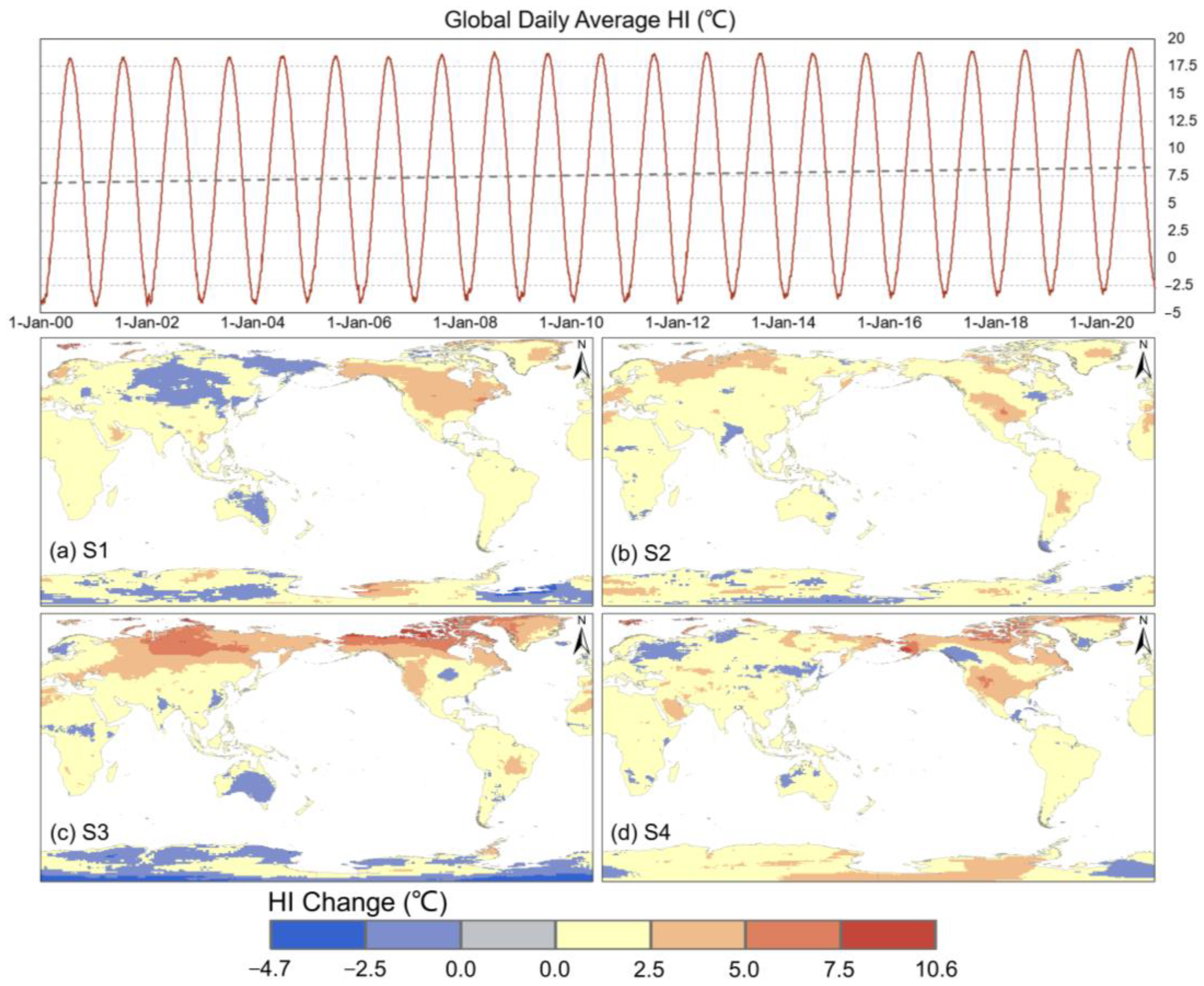
The global average daily HI exhibited a persistent upward trend since 2000 as shown in Figure 2, surpassing regular fluctuations and registering an approximate increase of 1.5 °C by 2020. Moreover, both the annual mean maximum HI and minimum HI over global land areas indicated a gradual ascent. Global HI change between 2000 and 2020 was initially obtained by rasterizing the difference between the HI calculation results and its spatial distribution is shown in Figure 2. Global HI varied significantly from season to season over the 20-year period but increased in the majority of land areas. There were similarities in the distribution of HI changes in different seasons, and the degree of HI changes from season to season was closely related to latitude, with most land areas near the equator, such as southern China, Southeast Asia, southern Mexico, and northern South America, showing small increases (0–1.4 °C) and less influenced by seasonal changes. The HI increased moderately (0–2.8 °C) in all four quarters in central Brazil, the Arabian Peninsula, and the Middle East, but increased slightly (0–1.4 °C) in S1, S2, and S4. In southeastern China, the HI decreased slightly (0–1.4 °C) in S3. The HI displayed a slight decrease (0–1.4 °C) in S1 and S3 in most of Australia (0–1.4 °C) and a small increase (0–1.4 °C) in S2 and S4. Change in HI in the middle and high latitudes was most influenced by the seasons, with the most significant difference in the change in northern China, Russia, northern Canada, the northern United States, and the Antarctic continent, and the HI decreased (0–1.4 °C) in S1 and S4 in northern China, and increased slightly (0–1.4 °C) in S2 and S3 (0–1.4 °C). The central and eastern regions of Russia showed a moderate decrease in the HI in S1 (0–2.6 °C) and a moderate or large increase in S2, S3, and S4 (1.4–4.2 °C). The eastern regions of Europe show a decrease in the HI in S4 (0–1.4 °C) and an increase in S1, S2, and S3 (0–1.4 °C). In most of the regions in Antarctica, the HI decreased in S1 and S3 (0–1.4 °C) and increased in S2 and S4 (0–1.4 °C). The HI increased significantly in S3 in northern Canada (1.4–5.9 °C) and decreased in S4 in the western region (0–1.4 °C). In the northern region of the United States, the HI decreased in S3 (0–1.4 °C) and increased in S1, S2, and S4 (0–2.8 °C). Thus, the change in global HI from season to season is more and more obvious with increasing latitude.

3.1.2. Global Heatwave Risk

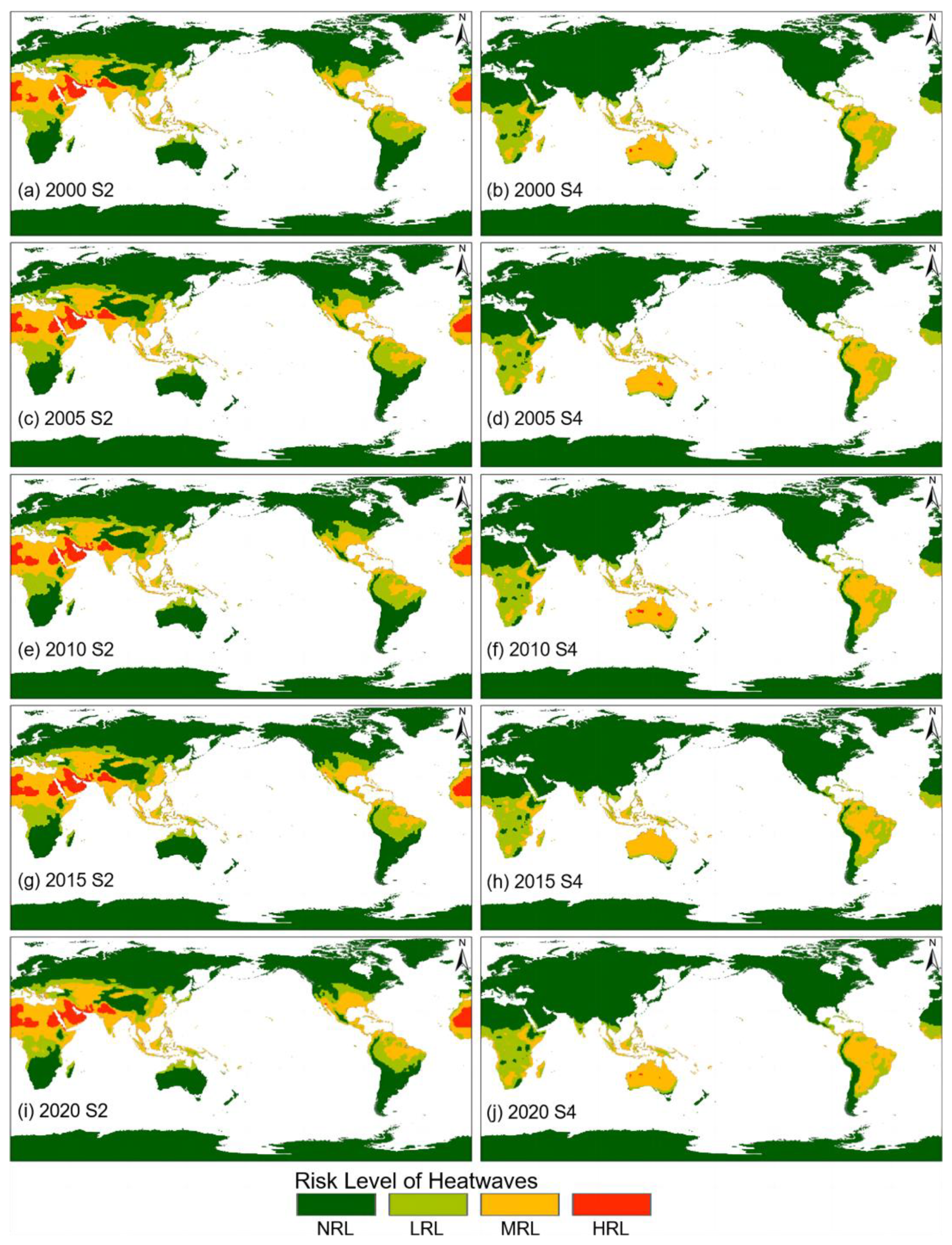
After reclassifying global HI according to the criteria, the global average number of days under each of the four different heatwave risk levels for each year from 2000 to 2020 is shown in Figure 3A; these time series were fitted by ordinary least squares regression with the highest R-squared fit chosen, and all passed the significance test with p-values less than 0.05. S2 (northern hemisphere summer) and S4 (southern hemisphere summer) were selected as representatives to obtain the global heatwave risk distribution during 2000–2020 as shown in Figure 4, and the number of pixels of each risk level and the area share are shown in Figure 3B. During the 20-year duration, a noteworthy inclination was observed towards a rise in the frequency of days characterized by an elevated risk level, with the exception of NRL days. The rate of decline in NRL days was the greatest (approximately 78.5 days Mkm−2), followed by the rate of increase in LRL days (approximately 42.6 days Mkm−2), the rate of increase in MRL days (approximately 31.5 days Mkm−2), and the rate of increase in HRL days was the slowest but also reached about 1-day Mkm−2. Within the global land area, the area under different risk levels of heatwaves in S2 and S4 varied greatly, among which the area under NRL was the largest, reaching more than 70% in S2 and more than 80% in S4. Among the remaining land areas, the proportion of high-risk areas was relatively small, less than 1% in S4 and only about 3% in S2. Meanwhile, in S2, the area of medium-risk region was slightly larger than low-risk, while in S4 the area of medium-risk region gradually increased from smaller than the area of low-risk region to larger than the area of low-risk. From 2000 to 2020, the proportion of no-risk and low-risk areas tended to gradually decrease, with the weakest change between 2005 and 2010, while the proportion of medium-risk and high-risk areas tended to gradually increase, showing the overall trend that global heatwave events are gradually worsening.
In S2, global heatwave risk areas were concentrated in the northern hemisphere at low latitudes and near the equator, while in S4 the opposite was true, with global heatwave risk areas concentrated in the southern hemisphere at low latitudes and near the equator. Some mid- and high-latitude land masses were still covered by risk-free areas globally, including Antarctica, which is always risk-free, Russia, which is closer to the Arctic, and most of Europe and northern North America, high-altitude areas in China such as the Qinghai-Tibet and Yunnan-Guizhou plateaus, and Australia and areas in southern Africa and southern South America, which were also risk-free. The areas under HRL are small in size and scattered in longitude, but they are all concentrated between the equator and the Tropic of Cancer in latitude. In S2, the high-risk areas were mainly located in the northern part of Africa, such as Saudi Arabia, Egypt, Sudan, and Mali, and the southwestern part of Asia, such as Pakistan and India; in S4, the high-risk areas were mainly located in the southern part of Africa, the Oceania region, such as the western part of Australia, and the central part of Brazil in South America. Most of these areas are controlled by the subtropical high-pressure zone, with prevailing sinking air currents, low precipitation throughout the year, hot and dry, prone to extreme heat disasters, and distributed with a large number of high-risk areas. Similarly, areas near the equator in S2 and S4 were distributed in high-risk areas, such as the northern regions of South America, Southeast Asia, and central Africa, as most of these areas are controlled by the tropical depression, humid and rainy, high temperatures throughout the year, the risk of extreme heatwave disasters is higher. Around these high-risk areas, there was a relatively continuous distribution of medium-risk areas, such as almost all the remaining land areas in central to northern Africa except Ethiopia, southwestern Asia, the Middle East, southern India, southeastern China, Southeast Asia, and parts of southern North America and northern South America. Low-risk areas of comparable size to medium-risk areas were distributed around the medium-risk areas. The change over the period 2000–2020 shows that the high-risk areas were gradually expanding in size, and the medium-risk areas were expanding outward while some of them were transformed into high-risk areas, and the area expanded was larger than the area transformed into high-risk areas. The low-risk areas were also expanding in the same way as the medium-risk areas, while the area of the no-risk areas was gradually decreasing due to the expansion of the peripheral areas of the low-risk areas.
The results of the change and shift analysis of global heatwave risk level for the period 2000–2020 are shown in Figure 5. As displayed in Figure 5A, the risk level did not change significantly in most regions during the 20-year period, while almost all of the regions that did change experienced an increase in risk level. Only a very small portion of western China and central Africa experienced a decrease in risk level in S2. In Asia and north-central Africa, the areas with upgraded risk levels were more scattered, while in central to southern North America and central to northern South America, the areas with upgraded risk levels were more concentrated and continuous, and larger in size. In S4, only a very small part of southern Africa and western Australia had a decrease in risk level, while central, western, and southern Africa had an increase in risk level with a more scattered distribution; Australia had a smaller area with an increase in risk level, and South America had a more concentrated area with a larger area with an increase in risk level. At the same time, central Africa, southern India, Southeast Asia, and South America all had areas with upgraded risk levels in S2 and S4.
The shift in the global heatwave risk level between S2 and S4 of 2000–2020 provides a better visualization of the change in risk level by region (Figure 5B). Antarctica and the land areas near the North and South Poles remained free of heatwave risk for 20 years, with some areas near the edges of the region converting from no-risk to low-risk. In S2, the distribution of risk areas extended to high latitudes in the northern hemisphere, and the high-risk areas in northern Africa and parts of southern Asia remained under HRL, with almost no reduction in risk level, and only a certain area on the periphery of the area from MRL to HRL. Compared with S2, the distribution of risk areas in the northern hemisphere was greatly reduced in S4, but the risk areas in the southern hemisphere at low latitudes and the shift in risk level did not change significantly compared with S2. In both seasons, there were almost no areas around the perennial medium-risk areas that were downgraded to low-risk areas, and some areas that were upgraded from low-risk to medium-risk areas were distributed in the periphery, and the area of such grade-changing areas accounted for the largest area among the grade-changing areas, i.e., the majority of the areas with upgraded risk levels had an excessive shift from LRL to MRL, and in both seasons, the shift was most obvious in the northern part of South America. The most significant transition occurred in the northern region of South America.

3.2. Attribution of Global Heatwaves

3.2.1. Single Driving Factor

The regression of the RF model for each driving factor as the explanatory variable of the global heatwaves was performed separately and the results are shown in Figure 6. All the results of the factor detection passed the significance test except for slope and NTL, and the explanatory power of different driving factors, i.e., the fit of the RF regression model (R2), differed significantly between 0 and 0.8.
The explanatory power of each factor for the heatwaves distribution during 2000–2020 shows a certain periodicity on the seasonal scale, with some factors having the greatest explanatory power in the first quarter (land use, precipitation) and others in the second quarter (slope direction, population density, elevation, slope, nighttime lights). With the increase of years, the explanatory power of each factor for the distribution of heatwaves does not vary much, and the R2 only changes very slightly, but the overall performance is slightly reduced, which indicates that the explanatory power of the seven abovementioned factors for the distribution of heatwaves tends to gradually decrease with time. The spatial distribution of heatwaves does not tend to be random, so there are still other factors that have more control over the distribution of global heatwaves to be explored, and the dominant factors affecting the spatial distribution of heatwaves also need to be explored.
Among all factors, the aspect had the greatest explanatory power (0.69–0.76) for the spatial distribution of the global heatwaves, followed by LUCC, with model fits ranging from 0.48 to 0.55. As the direction a slope faces, aspect affects the amount of sunlight it receives, and consequently, the temperature and humidity of the slope. North-facing slopes in the northern hemisphere (or south-facing slopes in the southern hemisphere) receive less direct sunlight compared to their counterparts, which results in lower temperatures and potentially lower relative humidity. Conversely, south-facing slopes in the northern hemisphere (or north-facing slopes in the southern hemisphere) receive more direct sunlight and tend to have higher temperatures and higher relative humidity. LUCC is the second most influential factor primarily because it directly affects the energy balance and microclimate characteristics of the Earth’s surface. Changes in land use, such as deforestation, agricultural expansion, or urbanization, can alter surface albedo, soil moisture, and vegetation cover, and create urban heat island effects. These alterations can lead to increased surface temperatures and changes in humidity, thus influencing the distribution of heatwave risks.
The explanatory power of precipitation fluctuated more with the season, reaching a maximum of 0.43. Precipitation significantly influences the global spatial distribution of heatwave risks as it affects atmospheric moisture, cloud cover, and evapotranspiration rates, which in turn impact temperature and humidity conditions. Higher precipitation can moderate temperatures through increased cloud cover and evapotranspiration, while lower precipitation can lead to higher temperatures and lower relative humidity, increasing heatwave risks.
The explanatory power of elevation and population density were comparable to each other, and both had some influence on the distribution of heatwaves, but the influence was relatively small. Although higher elevations generally experience cooler temperatures due to adiabatic cooling and lower atmospheric pressure, this relationship can vary significantly depending on other local and regional factors. For instance, regional climate, latitude, and local weather patterns can all play a role in determining the temperature at a specific elevation. Additionally, the influence of elevation on heatwave risks may be less uniform and more complex than other factors, making it harder to establish a consistent global pattern. Population density, on the other hand, is an indirect factor affecting heatwave risks. Higher population density could exacerbate the consequences of heatwaves, as more people are exposed to extreme heat, and urban heat island effects can intensify temperatures in densely populated areas. However, population density itself does not directly influence the formation or frequency of heatwaves; it primarily affects the vulnerability of communities to heat-related hazards.
The explanatory power of slope and NTL on the spatial distribution of global heatwaves was the smallest, especially NTL, which is almost zero, and could be judged to have nearly no effect on the distribution of global heatwaves. Slope can affect local temperature and humidity conditions to some extent. However, its influence on heatwave risks is less significant compared to factors such as aspect, land use, and precipitation, which have more direct and pronounced effects on temperature and humidity variations. The slope may play a more critical role in other hazard risks such as landslides or water runoff, but its connection to heatwave risks is generally weaker. Nighttime lights primarily serve as an indicator of human activity, energy consumption, and urbanization levels. While nighttime lights may have some indirect connections to phenomena such as the urban heat island effect and anthropogenic heat emissions, their role in causing or exacerbating heatwaves is relatively minor. Additionally, the spatial resolution of nighttime light data on a global scale might be limited, potentially failing to accurately capture local-scale temperature and humidity variations. Consequently, when analyzing the spatial distribution of heatwave risks, the influence of nighttime lights is considered negligible compared to other more critical factors.
From the seasonal perspective, the relative magnitude of the driving forces of each factor on the global heatwave distribution remained constant under different seasons, but there was still some influence of season on the explanatory power of each factor on the heatwave distribution. The average level of the explanatory power of each factor was relatively high in S1 and S2, followed by S3, while S4 was the lowest, probably because the spatial heterogeneity of global heatwaves is also less significant in that season, and the control power of each factor on its spatial distribution is also lower because it cannot be reflected. For example, the explanatory power of LUCC and precipitation factors were highest in S1 and lowest in S2, while the explanatory power of DEM, slope, aspect, and popdens was highest in S2 and lowest in S4. In numerous regions, S1 signified the transition from winter to spring, characterized by accelerated vegetation growth due to rising temperatures and precipitation. The influence of LUCC on heatwave risks may be more pronounced during this period, as alterations in land cover can directly affect local temperature and humidity conditions. Precipitation often exhibited greater variability during S1, with certain regions encountering elevated rainfall levels as they enter the wet season. This variability could engender a more robust association between precipitation and heatwave risks during S1 compared to other quarters. Conversely, S2 generally represents the zenith of the warm season in many areas, accompanied by more stable weather patterns and potentially less pronounced LUCC effects. The diminished variability in precipitation and land cover could account for the lower explanatory power of these factors during S2. Moreover, during S2, heightened solar radiation and predominantly clear skies can intensify the influence of topographical factors, such as DEM, slope, and aspect, on local temperature and humidity conditions. These factors may have a more substantial impact on heatwave risks during S2 due to more pronounced variations in solar exposure and shading effects. The elevated temperatures in S2 could culminate in an increased likelihood of heatwaves, potentially resulting in a stronger association between population density and heatwave risks, as higher population densities frequently correlate with urban heat island effects and anthropogenic heat emissions. In stark contrast, S4 was typified by colder temperatures and reduced solar radiation across various regions, which can attenuate the influence of topographical factors and population density on heatwave risks. Snow cover in certain areas may further mitigate the impact of slope and aspect on temperature and humidity conditions.
The explanatory power of each factor for the spatial distribution of the heatwaves varied little from year to year, with only minor fluctuations from 2000 to 2020, and the overall driving force of each factor showed a less significant decreasing trend. From the perspective of factors, although the seasonal variability of the explanatory power was large, the aspect was always the factor with the greatest explanatory power, followed by LUCC and precipitation. The relative magnitude of the explanatory power of popdens and DEM on the spatial distribution of heatwaves fluctuated, and the explanatory power of NTL and slope was always relatively small, almost close to zero, and the detection results were not significant.
After regressing all driving factors simultaneously as explanatory variables for heatwaves in an RF model, the importance ranking of each factor as an explanatory variable was obtained as sorted in Figure 7. In line with the conclusion of the regression of each factor in Figure 6, the aspect had the highest importance among all factors for the spatial distribution of the global heatwaves (34–43%), followed by LUCC (23–31%). The importance of precipitation fluctuated seasonally, reaching a maximum of about 21%, while DEM and popdens were of equal importance for the distribution of the heatwaves, both of which have some influence on its distribution, but both have small effects (5.7–11% and 3–18.8%). Slope and NTL had the least importance on the spatial distribution of the global heatwaves, especially NTL, which was almost 0%, and it could be indicated that NTL almost has no influence on the distribution of heatwaves compared with all the factors studied in this paper.

3.2.2. Interaction Driving Factors

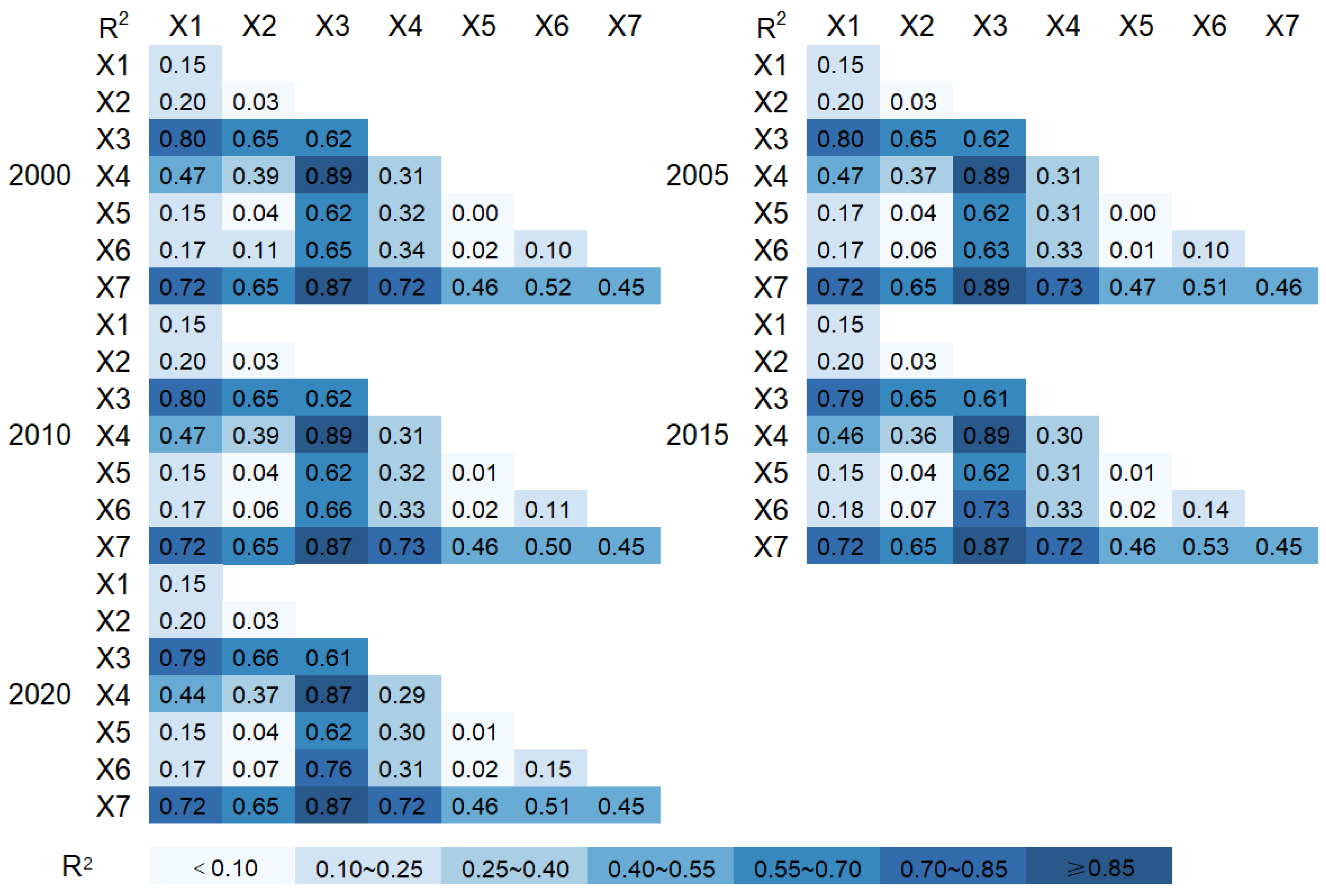
The RF regression of the interaction factors of global heatwaves was carried out on a time scale of years, and the R² of each RF regression model obtained is shown in Figure 8, listing the explanatory power of the distribution of global heatwaves after two-by-two interactions between the seven factors, and the factors represented by X1 to X7 can be found in Table 1. The interaction factor imputation results obtained for each year differed very little, and the R2 was in a fluctuating state with no significant trend. The explanatory power of most of the factors for global heatwave distribution did not decrease after an interaction.
Among them, the explanatory power of DEM increased significantly after interacting with precipitation and LUCC; especially after interacting with aspect, the explanatory power increased from 0.15 to 0.80. The interaction between DEM and precipitation can result in variations in temperature and humidity across different elevations. Higher elevations generally experience lower temperatures and increased precipitation due to orographic lift. The combined effect of elevation and precipitation can create localized microclimates that influence heatwave risks. Besides, the interaction between DEM and land use and LUCC can lead to variations in vegetation types and density across different elevations. Changes in land cover, such as deforestation or urbanization, can modify local temperature and humidity conditions and thus influence heatwave risks. When combined with the elevation data provided by DEM, these LUCC effects can be more accurately characterized, and their influence on heatwave risks is better understood. Aspect, or the direction a slope faces, affects the amount of solar radiation received by a given area, which influences temperature and humidity conditions. When DEM is combined with aspect, the resulting information can better represent the variations in solar exposure and potential microclimates that contribute to heatwave risks.
The single factor explanatory power of slope was only 0.03, which indicates almost no effect on the distribution of heatwaves, and reached 0.65 after interacting with aspect and LUCC, increasing the explanatory power. Slope, by itself, may have a limited impact on the distribution of heatwaves, as it does not take into account the direction the slope faces (i.e., aspect). When slope interacts with aspect, the combined information can better represent variations in solar exposure and shading effects across different terrains. Areas with a specific slope and aspect may receive more or less solar radiation, leading to differences in local temperature and humidity conditions. This interaction can help explain the distribution of heatwaves more effectively, resulting in an increase in explanatory power. Besides, when slope interacts with LUCC, it can better represent how different land use and land cover types are distributed across various terrains. For example, steeper slopes may have less vegetation or be less susceptible to urbanization compared to flatter areas, leading to different microclimates and heatwave risks. This interaction enables a more accurate representation of the spatial variability in microclimates and other environmental factors that contribute to heatwave distribution, thus enhancing the explanatory power.
The explanatory power of the aspect interacted with precipitation and LUCC for global heatwave distribution reached the maximum of all the interactions (above 0.85), but because the single-factor explanatory power of these two factors is already larger, the increase of the explanatory power of this interaction was still not as great as that of aspect and LUCC interacted with DEM and slope. However, the interaction of each factor with popdens and NTL has little effect on enhancing the explanatory power, and the model fit after the interaction has only a very small to negligible improvement compared with the single-factor model fit of the interacting factors. Popdens and NTL data often capture similar aspects of human activity and urbanization. Both factors can be indicative of the urban heat island effect, where built-up areas exhibit higher temperatures than surrounding rural areas. Since these factors provide overlapping information, their interaction with other factors might not add significant new insights, resulting in only a small improvement in explanatory power. The relationship between heatwave risks and factors such as popdens and NTL might not be consistent across different regions, resulting in spatial heterogeneity. In some areas, the urban heat island effect might be more pronounced, while in others, topographical and land cover factors might dominate. This spatial heterogeneity might weaken the overall increasing impact of interactions with population density and NTL on the explanatory power.

4. Discussion

In this paper, we analyzed the global seasonal-scale HI and heatwave risk from 2000 to 2020 and used RF model regression to analyze the explanatory power of seven factors on the global seasonal-scale heatwave distribution, including three topographic factors (DEM, slope, and aspect), one climatic factor (precipitation), and three human factors (NTL, popdens, and LUCC).

4.1. Global HI and Heatwave Risks

Over the past 20 years, global variations in seasonal HI have been observed, with most land areas experiencing an increase. Lower-latitude regions, such as southern China, Southeast Asia, southern Mexico, and northern South America, see smaller HI increases due to higher solar radiation and less seasonal impact. In contrast, the western and southern US, central Brazil, the Arabian Peninsula, and the Middle East show moderate or slight increases across all seasons, possibly related to atmospheric and oceanic circulation. Equatorial regions, influenced by the low-pressure belt, experience higher humidity and precipitation, limiting HI increases. Mid-to-high latitude regions exhibit more significant seasonal HI variations, affected by factors such as topography, land use, vegetation cover, and soil moisture. For instance, in northern China, HI decreases in the first and fourth quarters, while it increases in the second and third quarters due to the monsoon climate’s influence. Glaciers and snow cover also impact HI variations, particularly in polar regions and high mountain areas. In northern Canada’s third quarter and Alaska’s fourth quarter, substantial HI increases may result from seasonal climate changes, daylight hour variations, radiation intensity, polar amplification [72,73], monsoons, and climate system changes affecting temperature and precipitation distribution [74], as well as topography and land use type differences impacting climate characteristics and surface energy balance [12].
In scenarios S2 and S4, global heatwave risk areas displayed unique patterns, which could be influenced by factors such as atmospheric and oceanic circulation, climate zones, regional climate features, and climate change. Notably, in scenario S2, risks seemed to be concentrated in the northern hemisphere, specifically at low latitudes and near the equator. Conversely, scenario S4 appeared to predominantly focus on the southern hemisphere. Equatorial regions, typically characterized by humid and high-temperature environments, may face heightened heatwave risks. In contrast, subtropical high-pressure zones, known for their hot and dry conditions, could be more susceptible to extreme heat events. Climate change may play a role in the expansion of high- and medium-risk areas, causing regions that were previously considered low-risk to experience more frequent and intense heatwaves. A thorough and objective understanding of these factors is crucial for developing effective adaptation and mitigation strategies to address the growing challenges posed by heatwave risks.

4.2. Attribution of Global Heatwaves

Among the seven factors, all of them had some explanatory power for the spatial distribution of global heatwaves, except for slope and NTL, among which aspect had the greatest explanatory power, followed by LUCC and precipitation. The weakest explanatory power was from NTL (approximately 0), and there was almost no pattern between the global NTL distribution and the distribution of heatwaves after a comparative analysis of research data. On the one hand, some of the regions where extreme heatwave events occur, i.e., regions with high HI values, have harsh natural environments, such as the Sahara Desert in northern Africa, where very few people are able to adapt to survive and develop [75], and the NTL data used in this paper also showed that these regions have extremely low nighttime light value distributions; at the same time, the popdens and LUCC data used in this paper also showed that some of the regions with high HI values have extremely low population density and urban land area, resulting in only very weak or almost undetectable NTL distribution [76,77]. On the other hand, combined with the LUCC data used in this paper, some urban areas located in hot and humid climates and developed to a certain extent also have a higher risk of heatwaves due to their rapid urbanization [78], which corresponds to a distribution of high HI, and usually such areas also have a distribution of relatively high NTL values [79]. Therefore, the combination of the study data and the attribution results could indicate the possible reasons for the NTL data to be large without any driving force on the spatial distribution of global heatwaves.
Aspect demonstrates the greatest explanatory power for the global heatwave distribution, followed by LUCC and precipitation. Aspect plays a significant role in heatwave distribution due to its influence on solar radiation received by different slope directions, which in turn affects local temperature and humidity conditions [80,81]. In the Northern Hemisphere, south-facing slopes generally receive more solar radiation than north-facing slopes, which may lead to higher temperatures and lower relative humidity, thereby increasing the risk of heatwaves [82]. Similarly, east- and west-facing slopes may also exhibit different temperature and humidity characteristics, but further data analysis is needed to confirm this. LUCC also contributes to the heatwave distribution, as different land-cover types exhibit varied surface properties, such as albedo, evapotranspiration rates, and surface roughness, which can impact local microclimates and temperature patterns [83]. Urban areas, for instance, are known to experience higher temperatures and heatwave risks due to the urban heat island effect [59]. Precipitation has a weaker explanatory power for heatwave distribution, likely because it is more dependent on atmospheric circulation patterns and regional climate dynamics [84]. However, precipitation can still influence heatwave risks by modulating soil moisture and evaporative cooling, which in turn affects air temperature and humidity [85]. No significant trends in the time series were found in the R2 of the regression model for each influencing factor, indicating that the driving mechanism of each factor for the spatial distribution of the global heatwaves is relatively stable in time.

4.3. Possible Targeted Measures

This study described the spatial and temporal patterns of global heatwaves since the beginning of the 21st century. Through the analysis of meteorological data, the average body temperature in different regions and seasons was derived, and the changes in heatwave risk were analyzed, which could help people understand the current climate change situation and provide basic data support to promote policy design and risk reduction for climate change adaptation and disaster prevention and mitigation in various regions. Meanwhile, this study also analyzed the driving forces of different factors on global heatwave distribution, which could help the government and society to better understand the factors affecting climate change so that they can take corresponding preventive measures to mitigate the impact of heatwaves on human beings under climate change and promote the sustainable development of society. Based on the research findings, the following are some possible targeted suggestions for addressing heatwave risks:
Focus on changes in high-latitude areas: HI increase was found to be more pronounced in high-latitude areas, so greater attention should be given to heatwave risks and response measures in these regions;
Bolster land use and urban planning: As LUCC had significant explanatory power for the distribution of heatwaves, incorporating green infrastructure and low-carbon development strategies within urban planning and land use initiatives could effectively mitigate heatwave risks;
Consider the interplay between precipitation and heatwaves: Precipitation exhibited some explanatory power for the distribution of heatwaves. Thus, the relationship between precipitation and heatwaves should be taken into account to better predict and cope with heatwaves.
Utilize topographic information to optimize prevention measures: Since the results identified aspect as the primary explanatory factor for global heatwave distribution, employing topographic information when devising heatwave prevention measures can facilitate optimized resource allocation and response strategies;
Address seasonal variations: Tailoring response strategies to heatwave risks across different seasons is vital. For instance, during seasons with elevated heatwave risks, enhancing warning and emergency response systems can effectively raise public awareness and preparedness.

4.4. Limitations in Present Study

Following the definition and global study of Meehl et al. [12], Robinson et al. [68], Russo et al. [26], and Smith et al. [86], for the calculated HI, the risk levels of global extreme heatwaves were classified according to the value of the daily average HI as shown in Table 2, which is widely used and was derived based on historical data and climate models [87], as well as considerations of climate change and human adaptability in determining the thresholds [88]. This method directly reflects the combined impact on the human body, making it easy for the public to understand. Besides, by setting clear HI thresholds, the heatwave risk levels of different regions can be compared intuitively, which helps in formulating response measures. However, the absolute thresholds may still have limitations in terms of their applicability across different regions. These thresholds may provide an adequate division of heatwave risks in some areas but may not be as precise in others. Looking forward, our research plans include investigating the validity of the classification for different regions and considering comparative analyses that incorporate relative threshold divisions to refine and improve the heatwave risk classification method, making it more versatile and adaptable to a wider range of situations and regions.
Given the constraints posed by the limited data available at the spatial and temporal scales of this study, this paper only considered the influence of seven factors from topography, climate, and human aspects on the global seasonal heatwaves over a 20-year period from a geographic perspective. The underlying causes of the occurrence of heatwaves are still global warming, the influence of atmospheric circulation, the control of interplanetary elements, etc. There are other factors of greater mechanistic relevance available to perform the analysis of the driving forces at other spatiotemporal scales. In examining climatic factors, we primarily concentrated on the prevalent climatic variables that may exhibit associations with heatwaves. Initially, we selected relative humidity as a potential climatic factor, alongside precipitation, and obtained substantial explanatory power. However, considering that relative humidity was utilized as a variable in the calculation of the HI, we ultimately excluded it, presenting the final results with a single climatic factor. Nevertheless, it is crucial to acknowledge the potential influence of additional climatic variables. In future investigations, we will undoubtedly delve deeper into this subject, incorporating a broader range of climatic data to enhance our understanding. Additionally, human activities could also have an impact on heatwaves through their influence on surface temperature, urban heat island effect, etc., which is more complex, including urbanization, industrialization, transportation, etc., and also more difficult to accurately identify, quantify, directly access, and analyze. For example, the impact of transportation may be manifested in road traffic flow, pollutant emission, etc., and the impact of environmental aspects may be manifested in urban green coverage, building height and density, water bodies and forest area, etc. In the future, based on this study, we will try to overcome the above difficulties, obtain richer data sources, and analyze more comprehensively the mechanisms of the influence of more climatic meteorological and human factors on the spatiotemporal distribution and changes of heatwaves at different scales so as to propose more refined and regionally targeted interventions and policies for the prevention and control of extreme climate disasters.

5. Conclusions

Drawing upon near-surface air temperature and relative humidity data from ERA5 and a series of remote sensing products as driving factors, this study investigated the spatiotemporal variability of global human-perceived heatwaves on seasonal scales during 2000–2020. Considering the synergistic effect of temperature-humidity, HI was employed to characterize human health risks. An RF model regression was utilized to quantify the impact of various driving factors in topography, climate, and human activities, as well as the interactions between factors on the spatial distribution of global heatwaves. The key outcomes from the present study are summarized as follows:
  • Since the 21st century, changes in HI have varied significantly worldwide, with the majority of regions witnessing an increase, particularly at higher latitudes. The area of the HI-increasing region was larger in S2 and S4, and the largest HI-increasing area was observed in S2, while the overall HI increase peaked in S3;
  • Except for the decreasing area of no-risk regions, regions under all other risk levels expanded (the proportion of high-risk regions increased from 2.97% to 3.69% in S2, and from 0.04% to 0.35% in S4);
  • Aspect exhibited the most substantial influence on the spatial distribution of global heatwaves (0.69–0.76), followed by LUCC (0.48–0.55) and precipitation (0.16–0.43). In contrast, slope and NTL exhibited negligible effects, essentially having no impact on the global heatwave distribution;
  • From 2000 to 2020, the explanatory power of the factors underwent a minor decrease without a significant trend but showed seasonal periodicity. The overall explanatory power of each factor was relatively high in S1 and S2 and low in S4. The explanatory power of climatic and land use factors was the highest in S1, and that of topographic and other human factors was the highest in S2;
  • There was no significant trend in the attribution results of the interaction factors over the years, but the explanatory power of DEM and slope increased notably when interacting with the climate factor, aspect, and LUCC, respectively. The explanatory power of aspect and LUCC interacting with precipitation reached the maximum value (above 0.85) under all interactions.
Overall, these findings provide valuable insights into the changes in HI, human-perceived heatwave risks, and some underlying driving factors at a global scale, highlighting the interplay between climatic, topographic, and human factors in shaping heatwave patterns and risks.

Author Contributions

Conceptualization, Y.W. and N.Z.; methodology, Y.W. and N.Z.; software, Y.W.; validation, Y.W. and N.Z.; formal analysis, Y.W.; investigation, Y.W.; resources, Y.W.; data curation, Y.W.; writing—original draft preparation, Y.W.; writing—review and editing, N.Z.; visualization, Y.W.; supervision, N.Z.; project administration, N.Z.; funding acquisition, N.Z. All authors have read and agreed to the published version of the manuscript.

Funding

This research was supported by the Major Program of the National Natural Science Foundation of China (No. 42293270), the Program of Frontier Sciences of the Chinese Academy of Sciences (ZDBS-LY-DQC005), and the Key Project of Innovation LREIS (KPI001).

Data Availability Statement

All data used in the analysis are available in public repositories or upon request. The climate data from the ERA5 reanalysis dataset are available at https://cds.climate.copernicus.eu/cdsapp#!/search?type=dataset (accessed on 23 February 2023). Topographic data are provided by NASA at https://www.nasa.gov/ (accessed on 16 January 2023). Population density data are GPWv4 from NASA’s SEDAC available at https://sedac.ciesin.columbia.edu/data/set/gpw-v4-data-quality-indicators-rev11 (accessed on 27 December 2022). Nighttime light data are available on the Harvard Dataverse platform at https://doi.org/10.7910/DVN/YGIVCD (accessed on 16 January 2023). Global land use data are provided by the ESA at https://cds.climate.copernicus.eu/cdsapp#!/dataset/satellite-land-cover?tab=form (accessed on 19 January 2023).

Conflicts of Interest

The authors declare no conflict of interest.

References

  1. Mora, C.; Dousset, B.; Caldwell, I.R.; Powell, F.E.; Geronimo, R.C.; Bielecki, C.R.; Counsell, C.W.W.; Dietrich, B.S.; Johnston, E.T.; Louis, L.V.; et al. Global risk of deadly heat. Nat. Clim. Chang. 2017, 7, 501–506. [Google Scholar] [CrossRef] [Green Version]
  2. Watts, N.; Amann, M.; Arnell, N.; Ayeb-Karlsson, S.; Beagley, J.; Belesova, K.; Boykoff, M.; Byass, P.; Cai, W.; Campbell-Lendrum, D.; et al. The 2020 report of The Lancet Countdown on health and climate change: Responding to converging crises. Lancet 2020, 397, 129–170. [Google Scholar] [CrossRef]
  3. Carleton, T.; Jina, A.; Delgado, M.; Greenstone, M.; Houser, T.; Hsiang, S.; Hultgren, A.; Kopp, R.E.; McCusker, K.E.; Nath, I.; et al. Valuing the global mortality consequences of climate change accounting for adaptation costs and benefits. Q. J. Econ. 2022, 137, 2037–2105. [Google Scholar] [CrossRef]
  4. Burke, M.; Hsiang, S.M.; Miguel, E. Global non-linear effect of temperature on economic production. Nature 2015, 527, 235–239. [Google Scholar] [CrossRef] [PubMed]
  5. Dunne, J.P.; Stouffer, R.J.; John, J.G. Reductions in labour capacity from heat stress under climate warming. Nat. Clim. Chang. 2013, 3, 563–566. [Google Scholar] [CrossRef]
  6. Sun, Q.; Miao, C.; Hanel, M.; Borthwick, A.G.; Duan, Q.; Ji, D.; Li, H. Global heat stress on health, wildfires, and agricultural crops under different levels of climate warming. Environ. Int. 2019, 128, 125–136. [Google Scholar] [CrossRef] [PubMed]
  7. Ye, D.; Yin, J.; Chen, Z.; Zhen, Y.; Wu, R. Spatiotemporal Change Characteristics of Summer Heatwaves in China in 1961–2010. Adv. Clim. Chang. Res. 2013, 9, 15–20. [Google Scholar]
  8. Perkins, S.E.; Alexander, L.V.; Nairn, J.R. Increasing frequency, intensity and duration of observed global heatwaves and warm spells. Geophys. Res. Lett. 2012, 39, L20714. [Google Scholar] [CrossRef]
  9. Sun, Y.; Zhang, X.; Zwiers, F.W.; Song, L.; Wan, H.; Hu, T.; Yin, H.; Ren, G. Rapid increase in the risk of extreme summer heat in Eastern China. Nat. Clim. Chang. 2014, 4, 1082–1085. [Google Scholar] [CrossRef]
  10. Mitchell, D.; Heaviside, C.; Vardoulakis, S.; Huntingford, C.; Masato, G.; Guillod, B.P.; Frumhoff, P.; Bowery, A.; Wallom, D.; Allen, M. Attributing human mortality during extreme heat waves to anthropogenic climate change. Environ. Res. Lett. 2016, 11, 074006. [Google Scholar] [CrossRef]
  11. Matthews, T.K.R.; Wilby, R.L.; Murphy, C. Communicating the deadly consequences of global warming for human heat stress. Proc. Natl. Acad. Sci. USA 2017, 114, 3861–3866. [Google Scholar] [CrossRef] [PubMed]
  12. Meehl, G.A.; Tebaldi, C. More intense, more frequent, and longer lasting heat waves in the 21st century. Science 2004, 305, 994–997. [Google Scholar] [CrossRef] [Green Version]
  13. Coffel, E.D.; Horton, R.M.; De Sherbinin, A. Temperature and humidity based projections of a rapid rise in global heat stress exposure during the 21st century. Environ. Res. Lett. 2018, 13, 014001. [Google Scholar] [CrossRef]
  14. Coffel, E.D.; de Sherbinin, A.; Horton, R.M.; Lane, K.; Kienberger, S.; Wilhelmi, O. The science of adaptation to extreme heat. In Resilience; Elsevier: Amsterdam, The Netherlands, 2018; pp. 89–103. [Google Scholar] [CrossRef]
  15. Alizadeh, M.R.; Adamowski, J.; Nikoo, M.R.; AghaKouchak, A.; Dennison, P.; Sadegh, M. A century of observations reveals increasing likelihood of continental-scale compound dry-hot extremes. Sci. Adv. 2020, 6, eaaz4571. [Google Scholar] [CrossRef]
  16. Chen, Y.; Zhai, P. Revisiting summertime hot extremes in China during 1961–2015: Overlooked compound extremes and significant changes. Geophys. Res. Lett. 2017, 44, 5096–5103. [Google Scholar] [CrossRef]
  17. Feng, Y.; Wang, H.; Sun, F.; Liu, W. Dependence of compound hot and dry extremes on individual ones across China during 1961–2014. Atmospheric Res. 2023, 283, 106553. [Google Scholar] [CrossRef]
  18. Wang, J.; Chen, Y.; Tett, S.F.B.; Yan, Z.; Zhai, P.; Feng, J.; Xia, J. Anthropogenically-driven increases in the risks of summertime compound hot extremes. Nat. Commun. 2020, 11, 528. [Google Scholar] [CrossRef] [PubMed] [Green Version]
  19. Wang, X.; Lang, X.; Jiang, D. Detectable anthropogenic influence on summer compound hot events over China from 1965 to 2014. Environ. Res. Lett. 2022, 17, 034042. [Google Scholar] [CrossRef]
  20. Kjellstrom, T.; Briggs, D.; Freyberg, C.; Lemke, B.; Otto, M.; Hyatt, O. Heat, human performance, and occupational health: A key issue for the assessment of global climate change impacts. Annu. Rev. Public Health 2016, 37, 97–112. [Google Scholar] [CrossRef] [Green Version]
  21. Willett, K.M.; Sherwood, S. Exceedance of heat index thresholds for 15 regions under a warming climate using the wet-bulb globe temperature. Int. J. Clim. 2010, 32, 161–177. [Google Scholar] [CrossRef]
  22. Chen, X.; Li, N.; Zhang, Z.; Liu, J.; Wang, F. Estimation of future global population exposure to heatwaves—Based on the heat stress index. Adv. Clim. Chang. Res. 2020, 16, 424–432. [Google Scholar]
  23. Chen, X.; Li, N.; Huang, C.; Liu, J.; Zhang, Z. Projection of heatwaves by the combined impact of humidity and temperature in China. Prog. Geogr. 2020, 39, 36–44. [Google Scholar] [CrossRef]
  24. Pal, J.S.; Eltahir, E.A.B. Future temperature in south west Asia projected to exceed a threshold for human adaptability. Nat. Clim. Chang. 2015, 6, 197–200. [Google Scholar] [CrossRef]
  25. Sylla, M.B.; Faye, A.; Giorgi, F.; Diedhiou, A.; Kunstmann, H. Projected heat stress under 1.5 °C and 2 °C global warming scenarios creates unprecedented discomfort for humans in West Africa. Earths Future 2018, 6, 1029–1044. [Google Scholar] [CrossRef] [Green Version]
  26. Russo, S.; Sillmann, J.; Sterl, A. Humid heat waves at different warming levels. Sci. Rep. 2017, 7, 7477. [Google Scholar] [CrossRef] [Green Version]
  27. Gao, X.-J.; Wu, J.; Shi, Y.; Wu, J.; Han, Z.-Y.; Zhang, D.-F.; Tong, Y.; Li, R.-K.; Xu, Y.; Giorgi, F. Future changes in thermal comfort conditions over China based on multi-RegCM4 simulations. Atmos. Ocean Sci. Lett. 2018, 11, 291–299. [Google Scholar] [CrossRef] [Green Version]
  28. Wang, Y.; Shi, P.; Zeng, L.; Xie, Q.; Wang, D. Interannual variation of vegetation and precipitation in Pearl River Basin during 1982–1999. J. Trop. Oceanogr. 2011, 30, 44–50. [Google Scholar]
  29. Wang, Z.; Chen, X.; Li, Y. Spatio-temporal changes of NDVI in the Pearl River Basin. Ecol. Sci. 2006, 25, 303–307,311. [Google Scholar]
  30. Jing, J.; Wang, Y.; Yin, M. Spatial and temporal variation of the vegetation cover along Pearl River Basin based on SPOT4-VGT. J. Guilin Univ. Technol. 2014, 34, 711–716. [Google Scholar]
  31. Breiman, L. Random forests. Mach. Learn. 2001, 45, 5–32. [Google Scholar] [CrossRef] [Green Version]
  32. Genuer, R.; Poggi, J.M.; Tuleau-Malot, C. Variable selection using random forests. Pattern Recognit. Lett. 2010, 31, 2225–2236. [Google Scholar] [CrossRef] [Green Version]
  33. Prasad, A.M.; Iverson, L.R.; Liaw, A. Newer classification and regression tree techniques: Bagging and random forests for ecological prediction. Ecosystems 2006, 9, 181–199. [Google Scholar] [CrossRef]
  34. Liu, X.; Zhang, X.; Kong, X.; Shen, Y.-J. Random Forest Model Has the Potential for Runoff Simulation and Attribution. Water 2022, 14, 2053. [Google Scholar] [CrossRef]
  35. Wang, Y.; Liu, X.; Shen, Y. Applicability of the random forest model in quantifying the attribution of runoff changes. Chin. J. Eco-Agric. 2022, 30, 864–874. [Google Scholar]
  36. Zeng, X.; Schnier, S.; Cai, X. A data-driven analysis of frequent patterns and variable importance for streamflow trend attribution. Adv. Water Resour. 2020, 147, 103799. [Google Scholar] [CrossRef]
  37. Guo, W.; Ni, X.; Mu, Y.; Liu, T.; Zhang, J. Detection and Attribution of Alpine Inland Lake Changes by Using Random Forest Algorithm. Remote Sens. 2023, 15, 1144. [Google Scholar] [CrossRef]
  38. Gao, Q.; Li, G.; Li, Z. Attribution of climate change and human activities to urban water level alterations and factors importance analysis in Central Taihu Basin. Urban Clim. 2021, 40, 101011. [Google Scholar] [CrossRef]
  39. Shi, Y.; Jin, N.; Ma, X.; Wu, B.; He, Q.; Yue, C.; Yu, Q. Attribution of climate and human activities to vegetation change in China using machine learning techniques. Agric. For. Meteorol. 2020, 294, 108146. [Google Scholar] [CrossRef]
  40. Zhu, P.; Abramoff, R.; Makowski, D.; Ciais, P. Uncovering the Past and Future Climate Drivers of Wheat Yield Shocks in Europe with Machine Learning. Earth’s Future 2021, 9, e2020EF001815. [Google Scholar] [CrossRef]
  41. Gu, W.; Vieira, A.R.; Hoekstra, R.M.; Griffin, P.M.; Cole, D. Use of random forest to estimate population attributable fractions from a case-control study of Salmonella enterica serotype Enteritidis infections. Epidemiol. Infect. 2015, 143, 2786–2794. [Google Scholar] [CrossRef] [Green Version]
  42. Liang, P.; Yang, J.; Wang, W.; Yuan, G.; Han, M.; Zhang, Q.; Li, Z. Deep Learning Identifies Intelligible Predictors of Poor Prognosis in Chronic Kidney Disease. IEEE J. Biomed. Health Inform. 2023, 27, 3677–3685. [Google Scholar] [CrossRef]
  43. Munck, N.; Njage, P.M.K.; Leekitcharoenphon, P.; Litrup, E.; Hald, T. Application of Whole-Genome Sequences and Machine Learning in Source Attribution of Salmonella Typhimurium. Risk Anal. 2020, 40, 1693–1705. [Google Scholar] [CrossRef]
  44. Tanui, C.K.; Benefo, E.O.; Karanth, S.; Pradhan, A.K. A Machine Learning Model for Food Source Attribution of Listeria monocytogenes. Pathogens 2022, 11, 691. [Google Scholar] [CrossRef] [PubMed]
  45. Huang, S.; Yu, L.; Cai, D.; Zhu, J.; Liu, Z.; Zhang, Z.; Nie, Y.; Fraedrich, K. Driving mechanisms of urbanization: Evidence from geographical, climatic, social-economic and nighttime light data. Ecol. Indic. 2023, 148, 110046. [Google Scholar] [CrossRef]
  46. Qin, G.; Meng, Z.; Fu, Y. Drought and water-use efficiency are dominant environmental factors affecting greenness in the Yellow River Basin, China. Sci. Total Environ. 2022, 834, 155479. [Google Scholar] [CrossRef] [PubMed]
  47. Wei, X.; Huang, S.; Huang, Q.; Liu, D.; Leng, G.; Yang, H.; Duan, W.; Li, J.; Bai, Q.; Peng, J. Analysis of Vegetation Vulnerability Dynamics and Driving Forces to Multiple Drought Stresses in a Changing Environment. Remote Sens. 2022, 14, 4231. [Google Scholar] [CrossRef]
  48. Jin, D.; Murray, P.J.; Xin, X.; Qin, Y.; Chen, B.; Qing, G.; Zhang, Z.; Yan, R. Attribution of explanatory factors for change in soil organic carbon density in the native grasslands of Inner Mongolia, China. J. Arid. Land 2018, 10, 375–387. [Google Scholar] [CrossRef] [Green Version]
  49. Zhang, Y.; Bai, H.; Su, K.; Huang, X.; Meng, Q.; Guo, S. Spatial variation of extreme temperature change on southern and northern slopes of Shaanxi section in Qinling Mountains during 1960–2013. Acta Geogr. Sin. 2018, 73, 1296–1308. [Google Scholar]
  50. Zhao, X.; Bian, T.; Ren, G.; Zhang, Y.; Han, Z. Possible impacts of geographical factors on long-term trends of extreme temperature indices over northern Xinjiang, China. Prog. Geogr. 2021, 40, 681–692. [Google Scholar] [CrossRef]
  51. Zhou, T.; Wang, Z.; Qin, H.; Zeng, Y. Remote sensing extraction of geothermal anomaly based on terrain effect correction. J. Remote Sens. 2020, 24, 265–276. [Google Scholar] [CrossRef]
  52. Xu, C.; Song, S.; Zhang, Y.; Cui, R. Study on the Relationship Between Temperature and other Meteorological Elements. J. Agric. Catastropholgy 2020, 10, 39–40+43. [Google Scholar]
  53. Yu, J.; Liu, J. Quantitative Analysis with Geographical Detector on the Influence Factor of Temperature Variation in Northeast China. Hubei Agric. Sci. 2015, 54, 4682–4687. [Google Scholar]
  54. He, M. Assessing Heat Wave Risk in Beijing by Multi-Source Remote Sensing. Master Dissertation, Nanjing University of Information Science and Technology, Nanjing, China, 2019. [Google Scholar]
  55. Huang, X.; Song, T.; Wang, B.; Zheng, D.; Qi, M. Study on the influence of land use evolution of scale, structure and pattern on urban thermal environment: A case study of Xi’an. Sci. Geogr. Sin. 2022, 42, 926–937. [Google Scholar]
  56. Pepin, N.; Lundquist, J. Temperature trends at high elevations: Patterns across the globe. Geophys. Res. Lett. 2008, 35, L14701. [Google Scholar] [CrossRef] [Green Version]
  57. Bolch, T.; Rohrbach, N.; Kutuzov, S. Identification of potentially dangerous glacial lakes in the northern Tien Shan. Nat. Hazards 2011, 50, 319–342. [Google Scholar] [CrossRef] [Green Version]
  58. Fischer, E.M.; Schär, C. Consistent geographical patterns of changes in high-impact European heatwaves. Nat. Geosci. 2010, 3, 398–403. [Google Scholar] [CrossRef]
  59. Oke, T.R. The energetic basis of the urban heat island. Q. J. R. Meteorol. Soc. 1982, 108, 1–24. [Google Scholar] [CrossRef]
  60. Luber, G.; McGeehin, M. Climate change and extreme heat events. Am. J. Prev. Med. 2008, 35, 429–435. [Google Scholar] [CrossRef]
  61. Weng, Q.; Lu, D.; Schubring, J. Estimation of land surface temperature–vegetation abundance relationship for urban heat island studies. Remote Sens. Environ. 2004, 89, 467–483. [Google Scholar] [CrossRef]
  62. Hersbach, H.; Bell, B.; Berrisford, P.; Biavati, G.; Horányi, A.; Muñoz Sabater, J.; Nicolas, J.; Peubey, C.; Radu, R.; Rozum, I.; et al. ERA5 monthly averaged data on single levels from 1940 to present. In Copernicus Climate Change Service (C3S) Climate Data Store (CDS); European Centre for Medium-Range Weather Forecasts: Reading, UK, 2023. [Google Scholar] [CrossRef]
  63. Tuholske, C.; Caylor, K.; Funk, C.; Verdin, A.; Sweeney, S.; Grace, K.; Peterson, P.; Evans, T. Global urban population exposure to extreme heat. Proc. Natl. Acad. Sci. USA 2021, 118, e2024792118. [Google Scholar] [CrossRef]
  64. Wang, Y.; Zhao, N.; Wu, C.; Quan, J.; Chen, M. Future population exposure to heatwaves in 83 global megacities. Sci. Total Environ. 2023, 888, 164142. [Google Scholar] [CrossRef] [PubMed]
  65. Wang, Y.; Zhao, N.; Yin, X.; Wu, C.; Chen, M.; Jiao, Y.; Yue, T. Global future population exposure to heatwaves. Environ. Int. 2023, 178, 108049. [Google Scholar] [CrossRef] [PubMed]
  66. Rothfusz, L.P. The Heat Index “Equation”; SR90-23; National Oceanic and Atmospheric Administration: Silver Spring, MD, USA, 1990. [Google Scholar]
  67. Steadman, R.G. The assessment of sultriness. Part I: A temperature-humidity index based on human physiology and clothing science. J. Appl. Meteorol. 1979, 18, 861–873. [Google Scholar] [CrossRef]
  68. Robinson, P.J. On the Definition of a Heat Wave. J. Appl. Meteorol. 2001, 40, 762–775. [Google Scholar] [CrossRef]
  69. Wang, J.; Hu, M.; Gao, B.; Fan, H.; Wang, J. A spatiotemporal interpolation method for the assessment of pollutant concentrations in the Yangtze River estuary and adjacent areas from 2004 to 2013. Environ. Pollut. 2019, 252, 501–510. [Google Scholar] [CrossRef]
  70. Liu, W.; Tang, Z.; Xia, Y.; Han, M.; Jiang, W. Identifying the key factors influencing Chinese carbon intensity using machine learning, the random forest algorithm, and evolutionary analysis. Acta Geogr. Sin. 2019, 74, 2592–2603. [Google Scholar]
  71. Xia, X.-S.; Chen, J.-J.; Wang, J.-J.; Cheng, X.-F. PM2.5 concentration influencing factors in china based on the random forest model. Environ. Sci. 2020, 41, 2057–2065. [Google Scholar]
  72. Cohen, J.; Screen, J.A.; Furtado, J.C.; Barlow, M.; Whittleston, D.; Coumou, D.; Francis, J.; Dethloff, K.; Entekhabi, D.; Overland, J.; et al. Recent Arctic amplification and extreme mid-latitude weather. Nat. Geosci. 2014, 7, 627–637. [Google Scholar] [CrossRef] [Green Version]
  73. Serreze, M.C.; Barry, R.G. Processes and impacts of Arctic amplification: A research synthesis. Glob. Planet. Chang. 2011, 77, 85–96. [Google Scholar] [CrossRef]
  74. Yao, T.D.; Thompson, L.; Yang, W.; Yu, W.S.; Gao, Y.; Guo, X.J.; Yang, X.X.; Duan, K.Q.; Zhao, H.B.; Xu, B.Q.; et al. Different glacier status with atmospheric circulations in Tibetan Plateau and surroundings. Nat. Clim. Chang. 2012, 2, 663–667. [Google Scholar] [CrossRef]
  75. Yang, H.; Xu, Y.; Tao, S.; Pan, J.; Liu, K.; Wu, M. Vulnerability to Heat Waves and Adaptation: A Summary. Sci. Technol. Rev. 2010, 28, 98–102. [Google Scholar]
  76. Doll, C.; Muller, J.; Elvidge, C. Night-time imagery as a tool for global mapping of socioeconomic parameters and greenhouse gas emissions. Ambio 2000, 29, 157–162. [Google Scholar] [CrossRef]
  77. Doll, C.N.; Muller, J.-P.; Morley, J.G. Mapping regional economic activity from night-time light satellite imagery. Ecol. Econ. 2006, 57, 75–92. [Google Scholar] [CrossRef]
  78. Deng, Z.; Zhang, Q.; Xu, J.; Chen, M.; Qing, S.; Zhang, S. Comparative Studies of the harm characteristic of Hot-dry Wind and High Temperature HeatWaves. Adv. Earth Sci. 2009, 24, 865–873. [Google Scholar]
  79. Ma, T. Spatiotemporal characteristics of urbanization in China from the perspective of remotely sensed big data of nighttime light. J. Geo-Inf. Sci. 2019, 21, 59–67. [Google Scholar]
  80. McCarthy, M.P.; Harpham, C.; Goodess, C.M.; Jones, P.D. Simulating climate change in UK cities using a regional climate model, HadRM3. Int. J. Clim. 2011, 32, 1875–1888. [Google Scholar] [CrossRef]
  81. Beniston, M. Climatic change in mountain regions: A review of possible impacts. Clim. Chang. 2003, 59, 5–31. [Google Scholar] [CrossRef]
  82. Pepin, N.; Bradley, R.S.; Diaz, H.F.; Baraer, M.; Caceres, E.B.; Forsythe, N.; Fowler, H.; Greenwood, G.; Hashmi, M.Z.; Liu, X.D.; et al. Elevation-dependent warming in mountain regions of the world. Nat. Clim. Chang. 2015, 5, 424–430. [Google Scholar] [CrossRef] [Green Version]
  83. Seto, K.C.; Fragkias, M.; Güneralp, B.; Reilly, M.K. A meta-analysis of global urban land expansion. PLoS ONE 2011, 6, e23777. [Google Scholar] [CrossRef]
  84. Trenberth, K.E.; Dai, A.; Rasmussen, R.M.; Parsons, D.B. The changing character of precipitation. Bull. Am. Meteorol. Soc. 2003, 84, 1205–1218. [Google Scholar] [CrossRef]
  85. Orth, R.; Seneviratne, S.I. Variability of soil moisture and sea surface temperatures similarly important for warm-season land climate in the community earth system model. J. Clim. 2017, 30, 2141–2162. [Google Scholar] [CrossRef]
  86. Smith, T.T.; Zaitchik, B.F.; Gohlke, J.M. Heat waves in the United States: Definitions, patterns and trends. Clim. Chang. 2012, 118, 811–825. [Google Scholar] [CrossRef] [PubMed] [Green Version]
  87. Anderson, G.B.; Bell, M.L. Heat Waves in the United States: Mortality risk during heat waves and effect modification by heat wave characteristics in 43 U.S. communities. Environ. Health Perspect. 2011, 119, 210–218. [Google Scholar] [CrossRef] [PubMed] [Green Version]
  88. Hondula, D.M.; Balling, R.C.; Vanos, J.K.; Georgescu, M. Rising temperatures, human health, and the role of adaptation. Curr. Clim. Chang. Rep. 2015, 1, 144–154. [Google Scholar] [CrossRef] [Green Version]
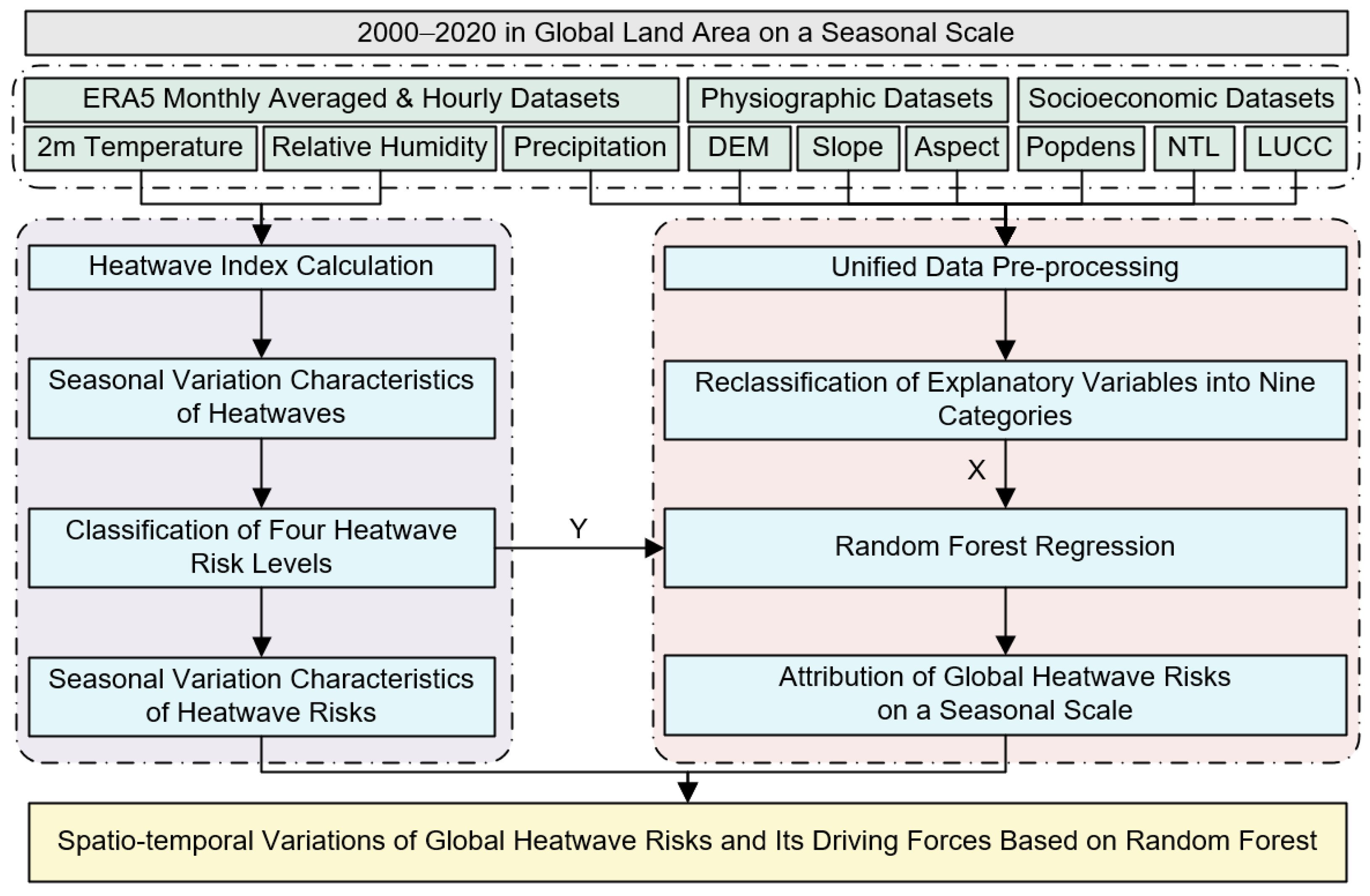
Figure 1. Technical roadmap.
Remotesensing 15 03627 g001
Figure 2. Changes in global HI in each season from 2000 to 2020: (a) in S1; (b) in S2; (c) in S3; and (d) in S4.
Remotesensing 15 03627 g002
Figure 3. The change in heatwave risks from 2000 to 2020. (A) Change in the average days under each risk level within a year from 2000 to 2020: (a) NRL; (b) LRL; (c) MRL; and (d) HRL. (B) Change in percentage of the area of each risk level in S2 and S4 from 2000 to 2020: (a) in S2; and (b) in S4.
Remotesensing 15 03627 g003
Figure 4. Distributions of risk levels of global extreme heatwaves in S2 and S4 from 2000 to 2020: (a) in S2 of 2000; (b) in S4 of 2000; (c) in S2 of 2005; (d) in S4 of 2005; (e) in S2 of 2010; (f) in S4 of 2010; (g) in S2 of 2015; (h) in S4 of 2015; (i) in S2 of 2020; and (j) in S4 of 2020.
Remotesensing 15 03627 g004
Figure 5. Change (A) and shift (B) in the risk level of global heatwaves in S2 and S4 from 2000 to 2020: (a) in S2; and (b) in S4.
Remotesensing 15 03627 g005
Figure 6. R2 of RF regression model of each single driving factor for global heatwaves in each season from 2000 to 2020. (A) Comparison of R2 of each single driving factor for global heatwaves in each season from 2000 to 2020: (a) in S1; (b) in S2; (c) in S3; and (d) in S4. (B) Change in R2 of each single driving factor for global heatwaves in each season from 2000 to 2020.
Remotesensing 15 03627 g006
Figure 7. Importance of each driving factor for global heatwaves of the total RF regression model in each season from 2000 to 2020: (a) in S1; (b) in S2; (c) in S3; and (d) in S4.
Remotesensing 15 03627 g007
Figure 8. R2 of RF regression model of each pair of interaction driving factors for global heatwaves from 2000 to 2020.
Remotesensing 15 03627 g008
Table 1. Factors selected to be detected in this study.
FactorDataTypeFactorDataType
X1DEMTopographicX5NTLhuman
X2SlopeTopographicX6popdenshuman
X3AspectTopographicX7LUCChuman
X4PrecipitationClimatic
Table 2. HI, the corresponding risk, and the health problems they could trigger.
HI (°F)HI (°C)Risk LevelHealth Impact
<80<26.7None (NRL)No significant effect
80~9026.7~32.2Low (LRL)Tiredness from prolonged exposure and/or physical work situations
90~10532.2~40.6Medium (MRL)Potential for spasms and vertigo with prolonged exposure and/or physical work
>105>40.6High (HRL)Likely to cause cramps, vertigo, and other symptoms, and may cause fainting or even life-threatening in prolonged exposure and/or physical work situations.
Disclaimer/Publisher’s Note: The statements, opinions and data contained in all publications are solely those of the individual author(s) and contributor(s) and not of MDPI and/or the editor(s). MDPI and/or the editor(s) disclaim responsibility for any injury to people or property resulting from any ideas, methods, instructions or products referred to in the content.