


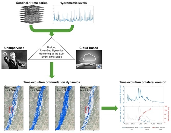
Monitoring Braided River-Bed Dynamics at the Sub-Event Time Scale Using Time Series of Sentinel-1 SAR Imagery


Abstract
1. Introduction
- (i)
- We incorporate water flow level information through metadata enrichment to facilitate the automatic extraction and monitoring of inundation dynamics at a sub-event temporal scale;
- (ii)
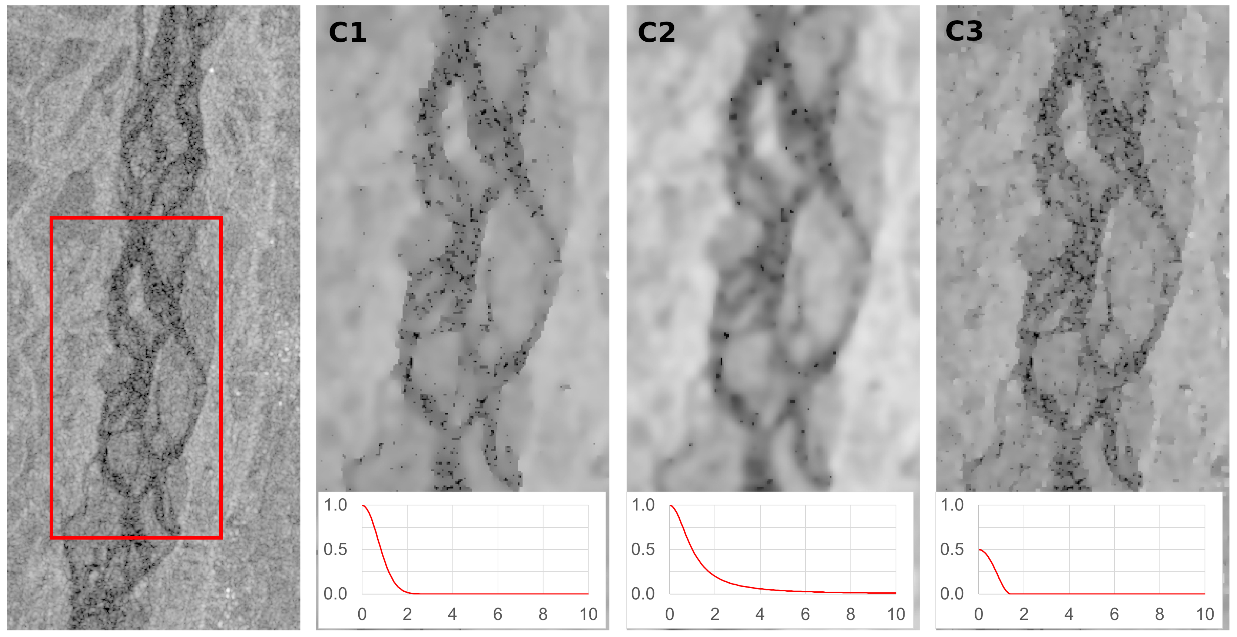
- We evaluate the denoising of speckle using three edge-stopping functions; and
- (iii)
- We apply a Self-Adaptive Thresholding Approach (SATA) based on the Otsu Algorithm.
2. Related Works
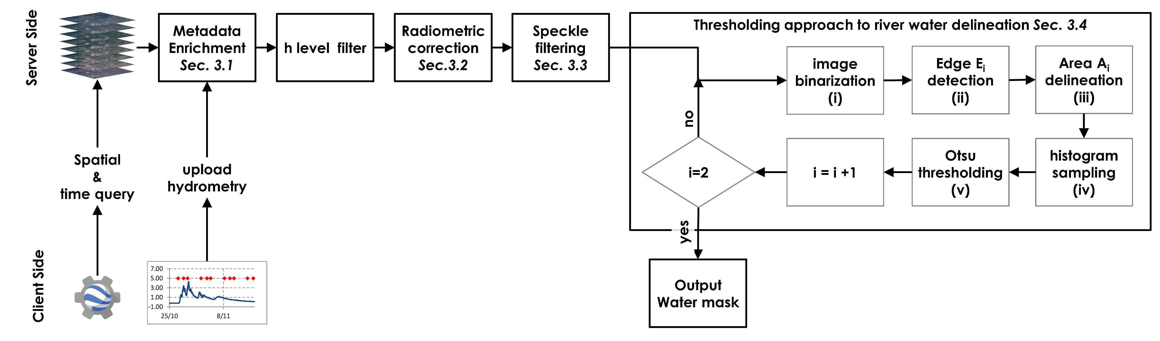
3. Materials and Methods
- Enriching the image stack with hydrometric data;
- Applying the radiometric slope correction algorithm;
- Reducing speckle noise;
- Extracting the wet channel with a Self-Adaptive Thresholding Approach; and
- Output functions.
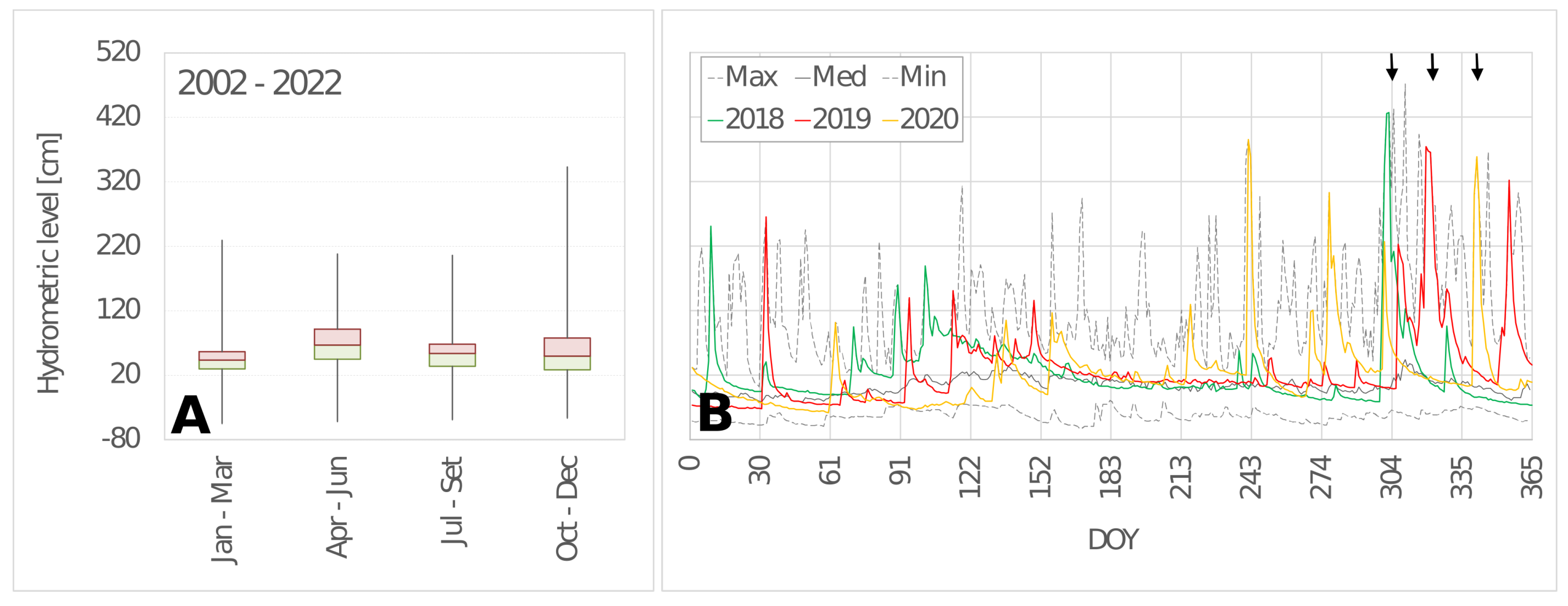
3.1. Image Selection and Metadata Enrichment
3.2. Radiometric Terrain Correction
3.3. Denoising
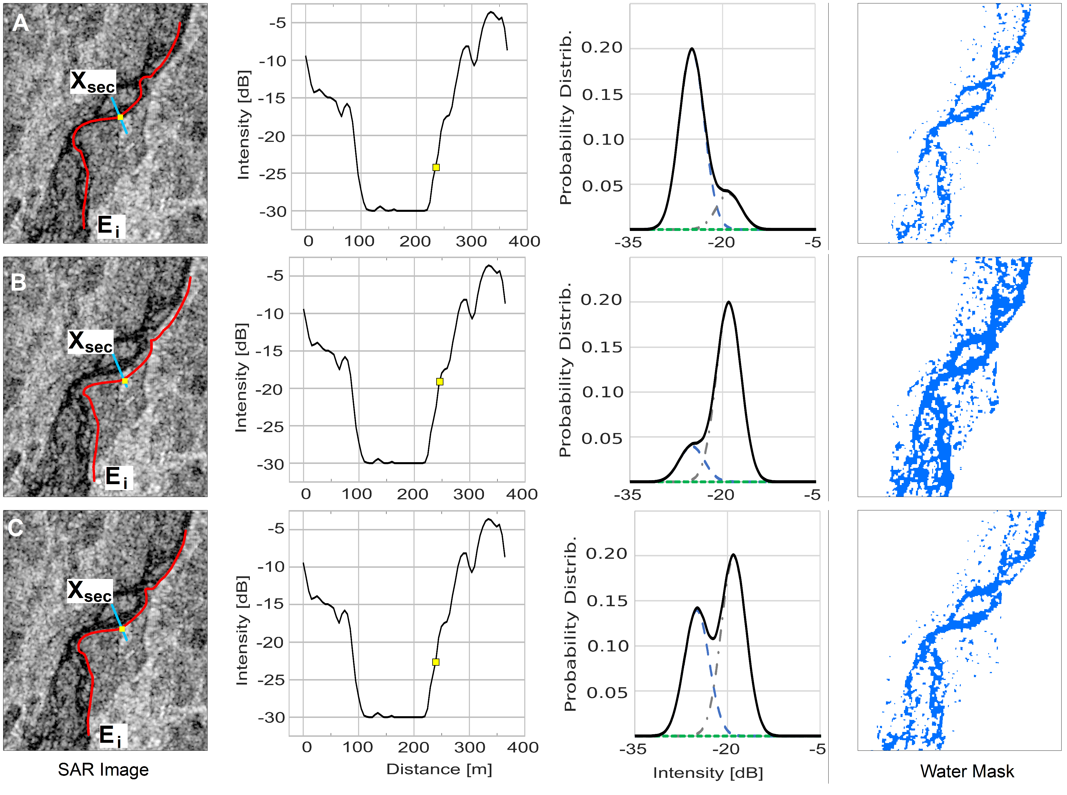
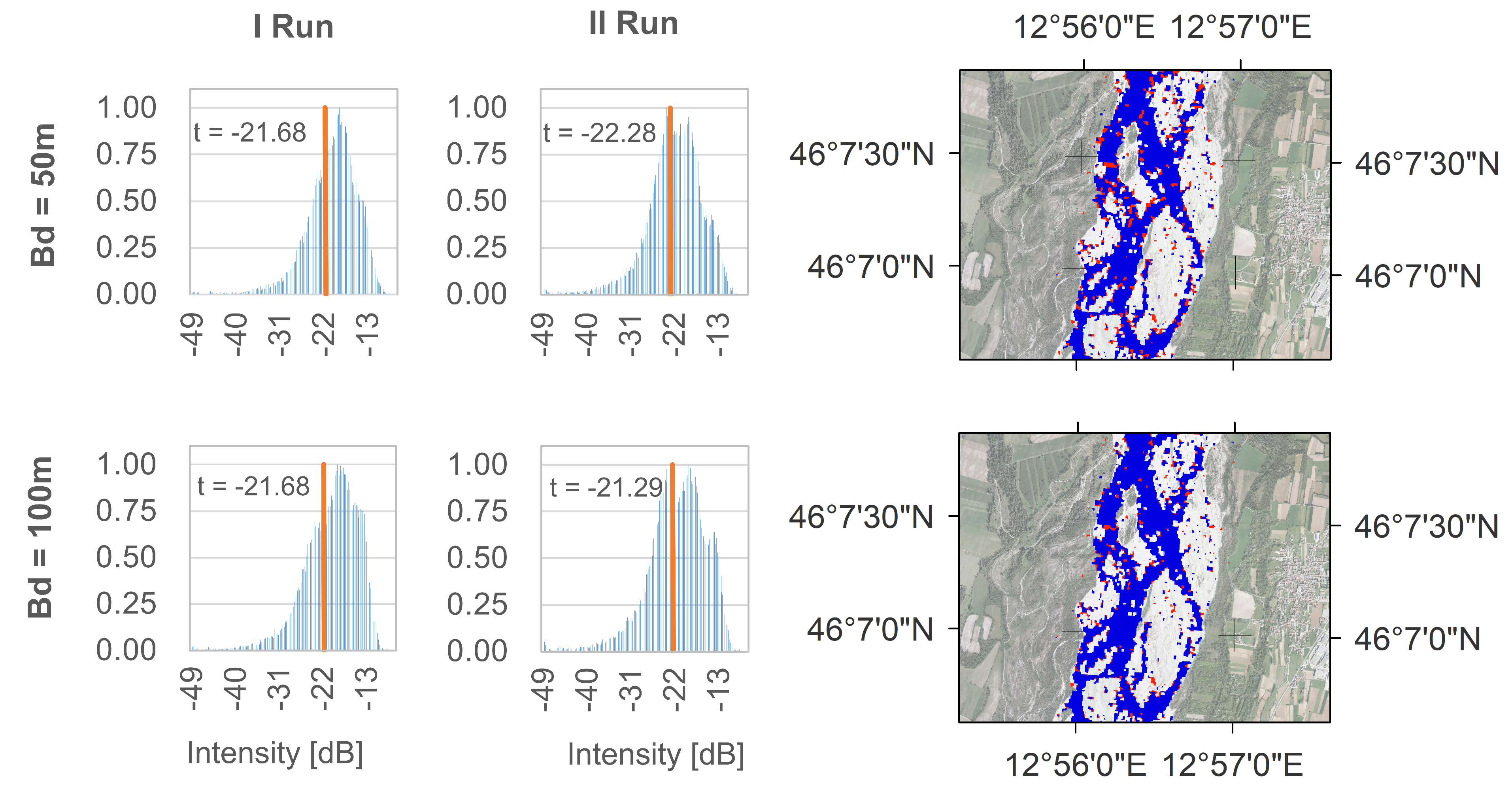
3.4. Self-Adaptive Thresholding Approach to River Water Delineation
- (i)
- Image binarization process using the threshold value t;
- (ii)
- Identification of the wet–dry edges E using the Canny Edge filter [75];
- (iii)
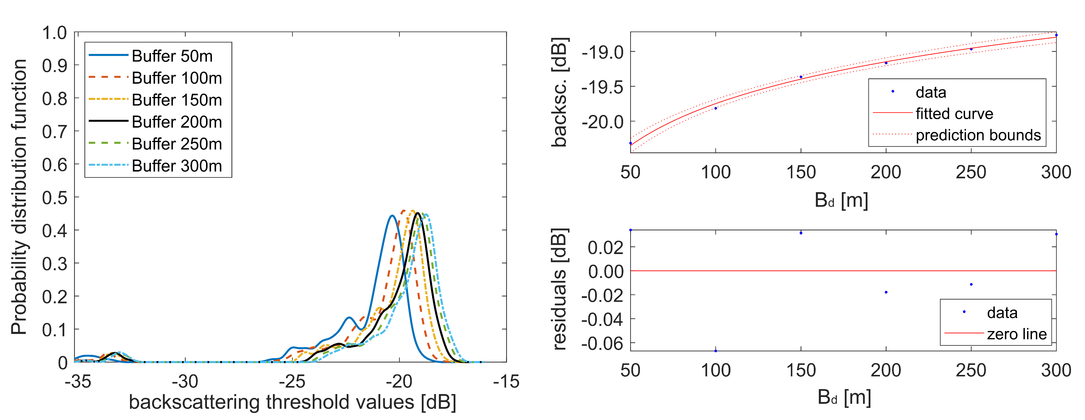
- Delineation of the area A applying a buffer (B) around the edges E;
- (iv)
- Histogram sampling within the area A;
- (v)
- Evaluation of the threshold t applying the Otsu algorithm.
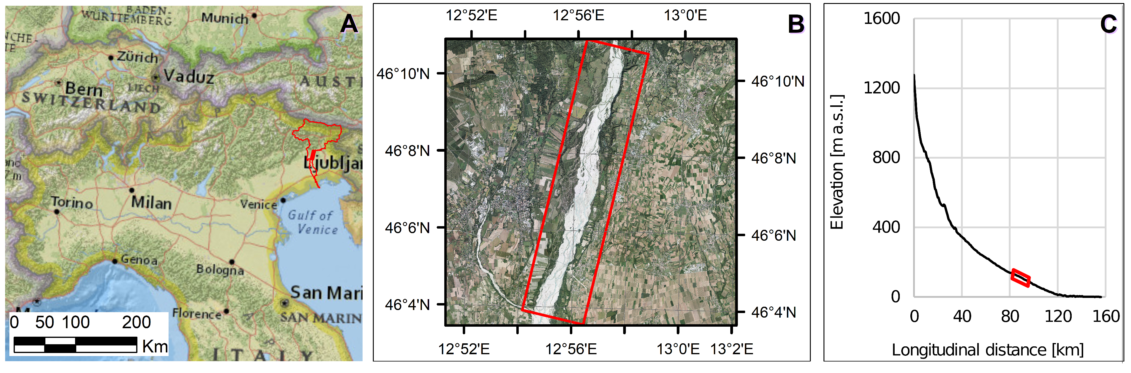
4. Case Study
5. Results
5.1. Sensitivity Analysis
5.2. Inundation Dynamics
6. Discussion and Conclusions
6.1. Potential Implications for Fluvial Geomorphology and River Management
6.2. Advantages, Limitations, and Further Development of the Proposed Procedure
Author Contributions
Funding
Data Availability Statement
Conflicts of Interest
References
- Anderson, E.P.; Jackson, S.; Tharme, R.E.; Douglas, M.; Flotemersch, J.E.; Zwarteveen, M.; Lokgariwar, C.; Montoya, M.; Wali, A.; Tipa, G.T.; et al. Understanding rivers and their social relations: A critical step to advance environmental water management. WIREs Water 2019, 6, e1381. [Google Scholar] [CrossRef] [PubMed]
- Petsch, D.K.; Cionek, V.d.M.; Thomaz, S.M.; dos Santos, N.C.L. Ecosystem services provided by river-floodplain ecosystems. Hydrobiologia 2022, 850, 2563–2584. [Google Scholar] [CrossRef]
- Tockner, K.; Stanford, J.A. Riverine flood plains: Present state and future trends. Environ. Conserv. 2002, 29, 308–330. [Google Scholar] [CrossRef]
- Fryiers, K.A.; Brierley, G.J. Geomorphic Analysis of River Systems. In Geomorphic Analysis of River Systems: An Approach to Reading the Landscape; John Wiley and Sons, Ltd.: Hoboken, NJ, USA, 2012; pp. 1–345. [Google Scholar] [CrossRef]
- Corenblit, D.; Tabacchi, E.; Steiger, J.; Gurnell, A.M. Reciprocal interactions and adjustments between fluvial landforms and vegetation dynamics in river corridors: A review of complementary approaches. Earth-Sci. Rev. 2007, 84, 56–86. [Google Scholar] [CrossRef]
- Sarker, S.; Sarker, T.; Leta, O.T.; Raihan, S.U.; Khan, I.; Ahmed, N. Understanding the Planform Complexity and Morphodynamic Properties of Brahmaputra River in Bangladesh: Protection and Exploitation of Riparian Areas. Water 2023, 15, 1384. [Google Scholar] [CrossRef]
- Phillips, J.D. Evolutionary geomorphology: Thresholds and nonlinearity in landform response to environmental change. Hydrol. Earth Syst. Sci. 2006, 10, 731–742. [Google Scholar] [CrossRef]
- Fryirs, K.A. River sensitivity: A lost foundation concept in fluvial geomorphology. Earth Surf. Process. Landf. 2017, 42, 55–70. [Google Scholar] [CrossRef]
- European Commission. Water Framework Directive. 2000. Available online: https://eur-lex.europa.eu/eli/dir/2000/60/oj (accessed on 1 January 2022).
- European Commission. Flood Directive. 2007. Available online: https://eur-lex.europa.eu/eli/dir/2007/60/oj (accessed on 1 January 2022).
- Tariq, M.A.U.R.; Farooq, R.; van de Giesen, N. A Critical Review of Flood Risk Management and the Selection of Suitable Measures. Appl. Sci. 2020, 10, 8752. [Google Scholar] [CrossRef]
- Powers, J.; Klemp, J.; Skamarock, W.; Davis, C.; Dudhia, J.; Gill, D.; Coen, J.; Gochis, D.; Ahmadov, R.; Peckham, S.; et al. The Weather Research and Forecasting (WRF) Model: Overview, System Efforts, and Future Directions. Bull. Am. Meteorol. Soc. 2017, 98, 1717–1737. [Google Scholar] [CrossRef]
- Giannaros, C.; Dafis, S.; Stefanidis, S.; Giannaros, T.; Koletsis, I.; Oikonomou, C. Hydrometeorological analysis of a flash flood event in an ungauged Mediterranean watershed under an operational forecasting and monitoring context. Meteorol. Appl. 2022, 29, e2079. [Google Scholar] [CrossRef]
- Piégay, H.; Arnaud, F.; Belletti, B.; Bertrand, M.; Bizzi, S.; Carbonneau, P.; Dufour, S.; Liébault, F.; Ruiz-Villanueva, V.; Slater, L. Remotely sensed rivers in the Anthropocene: State of the art and prospects. Earth Surf. Process. Landf. 2020, 45, 157–188. [Google Scholar] [CrossRef]
- Reichstein, M.; Camps-Valls, G.; Stevens, B.; Jung, M.; Denzler, J.; Carvalhais, N.; Prabhat, F. Deep learning and process understanding for data-driven Earth system science. Nature 2019, 566, 195–204. [Google Scholar] [CrossRef] [PubMed]
- Gomes, V.C.F.; Queiroz, G.R.; Ferreira, K.R. An Overview of Platforms for Big Earth Observation Data Management and Analysis. Remote Sens. 2020, 12, 1253. [Google Scholar] [CrossRef]
- Smith, L. Satellite remote sensing of river inundation area, stage, and discharge: A review. Hydrol. Process. 1997, 11, 1427–1439. [Google Scholar] [CrossRef]
- Pavelsky, T.M.; Smith, L.C. RivWidth: A Software Tool for the Calculation of River Widths From Remotely Sensed Imagery. IEEE Geosci. Remote Sens. Lett. 2008, 5, 70–73. [Google Scholar] [CrossRef]
- Monegaglia, F.; Zolezzi, G.; Güneralp, I.; Henshaw, A.J.; Tubino, M. Automated extraction of meandering river morphodynamics from multitemporal remotely sensed data. Environ. Model. Softw. 2018, 105, 171–186. [Google Scholar] [CrossRef]
- Pekel, J.F.; Cottam, A.; Gorelick, N.; Belward, A.S. High-resolution mapping of global surface water and its long-term changes. Nature 2016, 540, 418–4220. [Google Scholar] [CrossRef]
- Isikdogan, F.; Bovik, A.; Passalacqua, P. RivaMap: An automated river analysis and mapping engine. Remote Sens. Environ. 2017, 202, 88–97. [Google Scholar] [CrossRef]
- Spada, D.; Molinari, P.; Bertoldi, W.; Vitti, A.; Zolezzi, G. Multi-Temporal Image Analysis for Fluvial Morphological Characterization with Application to Albanian Rivers. ISPRS Int. J. Geo-Inf. 2018, 7, 314. [Google Scholar] [CrossRef]
- Brakenridge, G.R.; Knox, J.C.; Paylor, E.D.; Magilligan, F.J. Radar remote sensing aids study of the Great Flood of 1993. Eos Trans. Am. Geophys. Union 1994, 75, 521–527. [Google Scholar] [CrossRef]
- Smith, L.; Isacks, B.; Forster, R.; Bloom, A.; Preuss, I. Estimation of Discharge From Braided Glacial Rivers Using ERS 1 Synthetic Aperture Radar: First Results. Water Resour. Res. 1995, 31, 1325–1329. [Google Scholar] [CrossRef]
- Nykanen, D.; Foufoula-Georgiou, E.; Sapozhnikov, V. Study of spatial scaling in braided river patterns using synthetic aperture radar imagery. Water Resour. Res. 1998, 34, 1795–1808. [Google Scholar] [CrossRef]
- Dellepiane, S.; Angiati, E.; Vernazza, G. Processing and segmentation of COSMO-SkyMed images for flood monitoring. In Proceedings of the 2010 IEEE International Geoscience and Remote Sensing Symposium, Honolulu, HI, USA, 25–30 July 2010; pp. 4807–4810. [Google Scholar] [CrossRef]
- Pulvirenti, L.; Chini, M.; Pierdicca, N.; Guerriero, L.; Ferrazzoli, P. Flood monitoring using multi-temporal COSMO-SkyMed data: Image segmentation and signature interpretation. Remote Sens. Environ. 2011, 115, 990–1002. [Google Scholar] [CrossRef]
- Amitrano, D.; Di Martino, G.; Iodice, A.; Riccio, D.; Ruello, G. An end-user-oriented framework for the classification of multitemporal SAR images. Int. J. Remote Sens. 2016, 37, 248–261. [Google Scholar] [CrossRef]
- Amitrano, D.; Di Martino, G.; Iodice, A.; Riccio, D.; Ruello, G. Unsupervised Rapid Flood Mapping Using Sentinel-1 GRD SAR Images. IEEE Trans. Geosci. Remote Sens. 2018, 56, 3290–3299. [Google Scholar] [CrossRef]
- Papa, M.N.; Ruello, G.; Mitidieri, F.; Amitrano, D. Advanced Technologies for Satellite Monitoring of Water Resources. In Proceedings of the Frontiers in Water-Energy-Nexus—Nature-Based Solutions, Advanced Technologies and Best Practices for Environmental Sustainability, Salerno, Italy, 14–17 November 2018; Naddeo, V., Balakrishnan, M., Choo, K.H., Eds.; Springer International Publishing: Cham, Switzerland, 2020; pp. 157–160. [Google Scholar] [CrossRef]
- Mitidieri, F.; Papa, M.N.; Amitrano, D.; Ruello, G. River morphology monitoring using multitemporal SAR data: Preliminary results. Eur. J. Remote Sens. 2016, 49, 889–898. [Google Scholar] [CrossRef]
- Pulvirenti, L.; Marzano, F.S.; Pierdicca, N.; Mori, S.; Chini, M. Discrimination of Water Surfaces, Heavy Rainfall, and Wet Snow Using COSMO-SkyMed Observations of Severe Weather Events. IEEE Trans. Geosci. Remote Sens. 2014, 52, 858–869. [Google Scholar] [CrossRef]
- Pulvirenti, L.; Pierdicca, N.; Chini, M.; Guerriero, L. Monitoring Flood Evolution in Vegetated Areas Using COSMO-SkyMed Data: The Tuscany 2009 Case Study. IEEE J. Sel. Top. Appl. Earth Obs. Remote Sens. 2013, 6, 1807–1816. [Google Scholar] [CrossRef]
- Klemenjak, S.; Waske, B.; Valero, S.; Chanussot, J. Automatic Detection of Rivers in High-Resolution SAR Data. IEEE J. Sel. Top. Appl. Earth Obs. Remote Sens. 2012, 5, 1364–1372. [Google Scholar] [CrossRef]
- Ciecholewski, M. River channel segmentation in polarimetric SAR images: Watershed transform combined with average contrast maximisation. Expert Syst. Appl. 2017, 82, 196–215. [Google Scholar] [CrossRef]
- Zhou, S.; Kan, P.; Silbernagel, J.; Jin, J. Application of Image Segmentation in Surface Water Extraction of Freshwater Lakes using Radar Data. ISPRS Int. J. Geo-Inf. 2020, 9, 424. [Google Scholar] [CrossRef]
- Moharrami, M.; Javanbakht, M.H.; Attarchi, S. Automatic flood detection using sentinel-1 images on the google earth engine. Environ. Monit. Assess. 2021, 193, 248. [Google Scholar] [CrossRef] [PubMed]
- Donchyts, G.; Schellekens, J.; Winsemius, H.; Eisemann, E.; Van de Giesen, N. A 30 m Resolution Surface Water Mask Including Estimation of Positional and Thematic Differences Using Landsat 8, SRTM and OpenStreetMap: A Case Study in the Murray-Darling Basin, Australia. Remote Sens. 2016, 8, 386. [Google Scholar] [CrossRef]
- Chini, M.; Hostache, R.; Giustarini, L.; Matgen, P. A Hierarchical Split-Based Approach for Parametric Thresholding of SAR Images: Flood Inundation as a Test Case. IEEE Trans. Geosci. Remote Sens. 2017, 55, 6975–6988. [Google Scholar] [CrossRef]
- Cao, H.; Zhang, H.; Wang, C.; Zhang, B. Operational Flood Detection Using Sentinel-1 SAR Data over Large Areas. Water 2019, 11, 786. [Google Scholar] [CrossRef]
- Tan, J.; Tang, Y.; Liu, B.; Zhao, G.; Mu, Y.; Sun, M.; Wang, B. A Self-Adaptive Thresholding Approach for Automatic Water Extraction Using Sentinel-1 SAR Imagery Based on OTSU Algorithm and Distance Block. Remote Sens. 2023, 15, 2690. [Google Scholar] [CrossRef]
- Pai, M.M.; Mehrotra, V.; Aiyar, S.; Verma, U.; Pai, R.M. Automatic Segmentation of River and Land in SAR Images: A Deep Learning Approach. In Proceedings of the 2019 IEEE Second International Conference on Artificial Intelligence and Knowledge Engineering (AIKE), Sardinia, Italy, 3–5 June 2019; pp. 15–20. [Google Scholar] [CrossRef]
- Pai, M.; Mehrotra, V.; Verma, U.; Pai, R. Improved Semantic Segmentation of Water Bodies and Land in SAR Images Using Generative Adversarial Networks. Int. J. Semant. Comput. 2020, 14, 55–69. [Google Scholar] [CrossRef]
- Chen, L.; Zhang, P.; Xing, J.; Li, Z.; Xing, X.; Yuan, Z. A Multi-Scale Deep Neural Network for Water Detection from SAR Images in the Mountainous Areas. Remote Sens. 2020, 12, 3205. [Google Scholar] [CrossRef]
- Zhang, J.; Xing, M.; Sun, G.C.; Chen, J.; Li, M.; Hu, Y.; Bao, Z. Water Body Detection in High-Resolution SAR Images With Cascaded Fully-Convolutional Network and Variable Focal Loss. IEEE Trans. Geosci. Remote Sens. 2021, 59, 316–332. [Google Scholar] [CrossRef]
- Verma, U.; Chauhan, A.; Manohara, M.P.; Pai, R. DeepRivWidth: Deep learning based semantic segmentation approach for river identification and width measurement in SAR images of Coastal Karnataka. Comput. Geosci. 2021, 154, 104805. [Google Scholar] [CrossRef]
- Yuan, D.; Wang, C.; Wu, L.; Yang, X.; Guo, Z.; Dang, X.; Zhao, J.; Li, N. Water Stream Extraction via Feature-Fused Encoder-Decoder Network Based on SAR Images. Remote Sens. 2023, 15, 1559. [Google Scholar] [CrossRef]
- Amitrano, D.; Di Martino, G.; Iodice, A.; Riccio, D.; Ruello, G. A New Framework for SAR Multitemporal Data RGB Representation: Rationale and Products. IEEE Trans. Geosci. Remote Sens. 2015, 53, 117–133. [Google Scholar] [CrossRef]
- Obida, C.B.; Blackburn, G.A.; Whyatt, J.D.; Semple, K.T. River network delineation from Sentinel-1 SAR data. Int. J. Appl. Earth Obs. Geoinf. 2019, 83, 101910. [Google Scholar] [CrossRef]
- Twele, A.; Cao, W.; Plank, S.; Martinis, S. Sentinel-1-based flood mapping: A fully automated processing chain. Int. J. Remote Sens. 2016, 37, 2990–3004. [Google Scholar] [CrossRef]
- Jong-Sen Lee, E.P. (Ed.) Polarimetric Radar Imaging; CRC Press: Boca Raton, FL, USA, 2009. [Google Scholar] [CrossRef]
- Freeman, A. SAR calibration: An overview. IEEE Trans. Geosci. Remote Sens. 1992, 30, 1107–1121. [Google Scholar] [CrossRef]
- van Zyl, J.; Chapman, B.; Dubois, P.; Shi, J. The effect of topography on SAR calibration. IEEE Trans. Geosci. Remote Sens. 1993, 31, 1036–1043. [Google Scholar] [CrossRef]
- Ulander, L.M.H. Radiometric slope correction of synthetic-aperture radar images. IEEE Trans. Geosci. Remote Sens. 1996, 34, 1115–1122. [Google Scholar] [CrossRef]
- Luckman, A. Correction of SAR imagery for variation in pixel scattering area caused by topography. IEEE Trans. Geosci. Remote Sens. 1998, 36, 344–350. [Google Scholar] [CrossRef]
- Lee, J.S.; Schuler, D.; Ainsworth, T. Polarimetric SAR data compensation for terrain azimuth slope variation. IEEE Trans. Geosci. Remote Sens. 2000, 38, 2153–2163. [Google Scholar] [CrossRef]
- Hoekman, D.; Reiche, J. Multi-model radiometric slope correction of SAR images of complex terrain using a two-stage semi-empirical approach. Remote Sens. Environ. 2015, 156, 1–10. [Google Scholar] [CrossRef]
- Imperatore, P.; Di Martino, G. SAR Radiometric Calibration Based on Differential Geometry: From Theory to Experimentation on SAOCOM Imagery. Remote Sens. 2023, 15, 1286. [Google Scholar] [CrossRef]
- Hoekman, D.H. Radar Remote Sensing Data for Applications in Forestry; Wageningen University and Research: Wageningen, The Netherlands, 1990. [Google Scholar]
- Lee, J.S. Digital Image Enhancement and Noise Filtering by Use of Local Statistics. IEEE Trans. Pattern Anal. Mach. Intell. 1980, PAMI-2, 165–168. [Google Scholar] [CrossRef] [PubMed]
- Lee, J.S. Refined filtering of image noise using local statistics. Comput. Graph. Image Process. 1981, 15, 380–389. [Google Scholar] [CrossRef]
- Frost, V.S.; Stiles, J.A.; Shanmugan, K.S.; Holtzman, J.C. A Model for Radar Images and Its Application to Adaptive Digital Filtering of Multiplicative Noise. IEEE Trans. Pattern Anal. Mach. Intell. 1982, PAMI-4, 157–166. [Google Scholar] [CrossRef]
- Lopes, A.; Nezry, E.; Touzi, R.; Laur, H. Maximum A Posteriori Speckle Filtering Furthermore, First Order Texture Models In Sar Images. In Proceedings of the 10th Annual International Symposium on Geoscience and Remote Sensing, College Park, MD, USA, 20–24 May 1990; pp. 2409–2412. [Google Scholar] [CrossRef]
- Baraldi, A.; Parmiggiani, F. A refined gamma MAP SAR speckle filter with improved geometrical adaptivity. IEEE Trans. Geosci. Remote Sens. 1995, 33, 1245–1257. [Google Scholar] [CrossRef]
- Perona, P.; Malik, J. Scale-space and edge detection using anisotropic diffusion. IEEE Trans. Pattern Anal. Mach. Intell. 1990, 12, 629–639. [Google Scholar] [CrossRef]
- Lee, J.S. Digital image smoothing and the sigma filter. Comput. Vis. Graph. Image Process. 1983, 24, 255–269. [Google Scholar] [CrossRef]
- Lee, J.S.; Wen, J.H.; Ainsworth, T.L.; Chen, K.S.; Chen, A.J. Improved Sigma Filter for Speckle Filtering of SAR Imagery. IEEE Trans. Geosci. Remote Sens. 2009, 47, 202–213. [Google Scholar] [CrossRef]
- Argenti, F.; Lapini, A.; Bianchi, T.; Alparone, L. A Tutorial on Speckle Reduction in Synthetic Aperture Radar Images. IEEE Geosci. Remote Sens. Mag. 2013, 1, 6–35. [Google Scholar] [CrossRef]
- Singh, P.; Diwakar, M.; Shankar, A.; Pandey, R.S.; Kumar, M. A Review on SAR Image and its Despeckling. Arch. Comput. Methods Eng. 2021, 28, 4634–4653. [Google Scholar] [CrossRef]
- Baraha, S.; Sahoo, A.K.; Modalavalasa, S. A systematic review on recent developments in nonlocal and variational methods for SAR image despeckling. Signal Process. 2022, 196, 108521. [Google Scholar] [CrossRef]
- Hummel, R.; Moniot, R. Reconstructions from zero crossings in scale space. IEEE Trans. Acoust. Speech Signal Process. 1989, 37, 2111–2130. [Google Scholar] [CrossRef]
- Koenderink, J. The structure of images. Biol. Cybern. 1984, 50, 363–370. [Google Scholar] [CrossRef] [PubMed]
- Black, M.; Sapiro, G.; Marimont, D.; Heeger, D. Robust anisotropic diffusion. IEEE Trans. Image Process. 1998, 7, 421–432. [Google Scholar] [CrossRef] [PubMed]
- Guo, Z.; Wu, L.; Huang, Y.; Guo, Z.; Zhao, J.; Li, N. Water-Body Segmentation for SAR Images: Past, Current, and Future. Remote Sens. 2022, 14, 1752. [Google Scholar] [CrossRef]
- Canny, J. A Computational Approach to Edge Detection. IEEE Trans. Pattern Anal. Mach. Intell. 1986, PAMI-8, 679–698. [Google Scholar] [CrossRef]
- Otsu, N. A threshold selection method from gray level histograms. IEEE Trans. Syst. Man Cybern. 1979, 9, 62–66. [Google Scholar] [CrossRef]
- Kheradmandi, N.; Mehranfar, V. A critical review and comparative study on image segmentation-based techniques for pavement crack detection. Constr. Build. Mater. 2022, 321, 126162. [Google Scholar] [CrossRef]
- Tockner, K.; Ward, J.V.; Arscott, D.B.; Edwards, P.J.; Kollmann, J.; Gurnell, A.M.; Petts, G.E.; Maiolini, B. The Tagliamento River: A model ecosystem of European importance. Aquat. Sci. 2003, 65, 239–253. [Google Scholar] [CrossRef]
- Tarquini, S.; Isola, I.; Favalli, M.; Mazzarini, F.; Bisson, M.; Pareschi, M.; Boschi, E. TINITALY/01: A new triangular irregular network of Italy. Ann. Geophys. 2007, 50, 407–425. [Google Scholar] [CrossRef]
- Vollrath, A.; Mullissa, A.; Reiche, J. Angular-Based Radiometric Slope Correction for Sentinel-1 on Google Earth Engine. Remote Sens. 2020, 12, 1867. [Google Scholar] [CrossRef]
- Doering, M.; Uehlinger, U.; Rotach, A.; Schlaepfer, D.R.; Tockner, K. Ecosystem expansion and contraction dynamics along a large Alpine alluvial corridor (Tagliamento River, Northeast Italy). Earth Surf. Process. Landf. 2007, 32, 1693–1704. [Google Scholar] [CrossRef]
- van der Nat, D.; Schmidt, A.P.; Tockner, K.; Edwards, P.J.; Ward, J.V. Inundation Dynamics in Braided Floodplains: Tagliamento River, Northeast Italy. Ecosystems 2002, 5, 636–647. [Google Scholar] [CrossRef]
- Welber, M.; Bertoldi, W.; Tubino, M. The response of braided planform configuration to flow variations, bed reworking and vegetation: The case of the Tagliamento River, Italy. Earth Surf. Process. Landf. 2012, 37, 572–582. [Google Scholar] [CrossRef]
- Rinaldi, M.; Darby, S.E. 9 Modelling river-bank-erosion processes and mass failure mechanisms: Progress towards fully coupled simulations. Dev. Earth Surf. Process. 2007, 11, 213–239. [Google Scholar] [CrossRef]
- Farò, D.; Baumgartner, K.; Vezza, P.; Zolezzi, G. A novel unsupervised method for assessing mesoscale river habitat structure and suitability from 2D hydraulic models in gravel-bed rivers. Ecohydrology 2022, 15, e2452. [Google Scholar] [CrossRef]
- Best, J. Anthropogenic stresses on the world’s big rivers. Nat. Geosci. 2019, 12, 7–21. [Google Scholar] [CrossRef]
- Florsheim, J.L.; Mount, J.F.; Chin, A. Bank Erosion as a Desirable Attribute of Rivers. BioScience 2008, 58, 519–529. [Google Scholar] [CrossRef]
- Langhorst, T.; Pavelsky, T. Global Observations of Riverbank Erosion and Accretion From Landsat Imagery. J. Geophys. Res. Earth Surf. 2023, 128, e2022JF006774. [Google Scholar] [CrossRef]
- Boothroyd, R.J.; Williams, R.D.; Hoey, T.B.; Barrett, B.; Prasojo, O.A. Applications of Google Earth Engine in fluvial geomorphology for detecting river channel change. WIREs Water 2021, 8, e21496. [Google Scholar] [CrossRef]
- Bizzi, S.; Demarchi, L.; Grabowski, R.; Weissteiner, C.J.; Van de Bund, W. The use of remote sensing to characterise hydromorphological properties of European rivers. Aquat. Sci. 2016, 78, 57–70. [Google Scholar] [CrossRef]
- Clement, M.; Kilsby, C.; Moore, P. Multi-temporal synthetic aperture radar flood mapping using change detection. J. Flood Risk Manag. 2018, 11, 152–168. [Google Scholar] [CrossRef]
- Wu, X.; Zhang, Z.; Xiong, S.; Zhang, W.; Tang, J.; Li, Z.; An, B.; Li, R. A Near-Real-Time Flood Detection Method Based on Deep Learning and SAR Images. Remote Sens. 2023, 15, 2046. [Google Scholar] [CrossRef]
- Swain, P.; King, R. Two effective feature selection criteria for multispectral remote sensing. In Proceedings of the First International Joint Conference on Pattern Recognition, Mayflower Hotel, Washington, DC, USA, November 1973. [Google Scholar]
- Demirkaya, O.; Asyali, M.H. Determination of image bimodality thresholds for different intensity distributions. Signal Process. Image Commun. 2004, 19, 507–516. [Google Scholar] [CrossRef]
- Ashman, K.; Bird, C.M.; Zepf, S.E. Detecting Bimodality in Astronomical Datasets. arXiv 1994. [Google Scholar] [CrossRef]
- Hori, M. Near-daily monitoring of surface temperature and channel width of the six largest Arctic rivers from space using GCOM-C/SGLI. Remote Sens. Environ. 2021, 263, 112538. [Google Scholar] [CrossRef]
- Feng, M.; Zolezzi, G.; Pusch, M. Effects of thermopeaking on the thermal response of alpine river systems to heatwaves. Sci. Total Environ. 2018, 612, 1266–1275. [Google Scholar] [CrossRef]
- Swain, R.; Sahoo, B. Improving river water quality monitoring using satellite data products and a genetic algorithm processing approach. Sustain. Water Qual. Ecol. 2017, 9–10, 88–114. [Google Scholar] [CrossRef]
- Intajag, S.; Chitwong, S. Speckle Noise Estimation with Generalized Gamma Distribution. In Proceedings of the 2006 SICE-ICASE International Joint Conference, Busan, Republic of Korea, 18–21 October 2006; pp. 1164–1167. [Google Scholar] [CrossRef]
- Escamilla, H.M.; Méndez, E.R. Speckle statistics from gamma-distributed random-phase screens. J. Opt. Soc. Am. A-Opt. Image Sci. Vis. 1991, 8, 1929–1935. [Google Scholar] [CrossRef]
- Giustarini, L.; Vernieuwe, H.; Verwaeren, J.; Chini, M.; Hostache, R.; Matgen, P.; Verhoest, N.; De Baets, B. Accounting for image uncertainty in SAR-based flood mapping. Int. J. Appl. Earth Obs. Geoinf. 2015, 34, 70–77. [Google Scholar] [CrossRef]
- Chehibi, M.; Ferchichi, A.; Farah, I.R. Representing and modeling spatio-temporal uncertainty using belief function theory in flood extent mapping. Expert Syst. Appl. 2022, 209, 118212. [Google Scholar] [CrossRef]
- Giustarini, L.; Hostache, R.; Matgen, P.; Schumann, G.J.P.; Bates, P.D.; Mason, D.C. A Change Detection Approach to Flood Mapping in Urban Areas Using TerraSAR-X. IEEE Trans. Geosci. Remote Sens. 2013, 51, 2417–2430. [Google Scholar] [CrossRef]
- Chapman, B.; McDonald, K.; Shimada, M.; Rosenqvist, A.; Schroeder, R.; Hess, L. Mapping Regional Inundation with Spaceborne L-Band SAR. Remote Sens. 2015, 7, 5440–5470. [Google Scholar] [CrossRef]
- Pierdicca, N.; Chini, M.; Pulvirenti, L. Enhanced Land Cover and Flood Mapping at C- and L-BAND. In Proceedings of the IGARSS 2020—2020 IEEE International Geoscience and Remote Sensing Symposium, Waikoloa, HI, USA, 26 September–2 October 2020; pp. 4061–4064. [Google Scholar] [CrossRef]


Disclaimer/Publisher’s Note: The statements, opinions and data contained in all publications are solely those of the individual author(s) and contributor(s) and not of MDPI and/or the editor(s). MDPI and/or the editor(s) disclaim responsibility for any injury to people or property resulting from any ideas, methods, instructions or products referred to in the content. |
© 2023 by the authors. Licensee MDPI, Basel, Switzerland. This article is an open access article distributed under the terms and conditions of the Creative Commons Attribution (CC BY) license (https://creativecommons.org/licenses/by/4.0/).
Share and Cite
Rossi, D.; Zolezzi, G.; Bertoldi, W.; Vitti, A. Monitoring Braided River-Bed Dynamics at the Sub-Event Time Scale Using Time Series of Sentinel-1 SAR Imagery. Remote Sens. 2023, 15, 3622. https://doi.org/10.3390/rs15143622
Rossi D, Zolezzi G, Bertoldi W, Vitti A. Monitoring Braided River-Bed Dynamics at the Sub-Event Time Scale Using Time Series of Sentinel-1 SAR Imagery. Remote Sensing. 2023; 15(14):3622. https://doi.org/10.3390/rs15143622
Chicago/Turabian StyleRossi, Daniele, Guido Zolezzi, Walter Bertoldi, and Alfonso Vitti. 2023. "Monitoring Braided River-Bed Dynamics at the Sub-Event Time Scale Using Time Series of Sentinel-1 SAR Imagery" Remote Sensing 15, no. 14: 3622. https://doi.org/10.3390/rs15143622
APA StyleRossi, D., Zolezzi, G., Bertoldi, W., & Vitti, A. (2023). Monitoring Braided River-Bed Dynamics at the Sub-Event Time Scale Using Time Series of Sentinel-1 SAR Imagery. Remote Sensing, 15(14), 3622. https://doi.org/10.3390/rs15143622