The Detection of Green Tide Biomass by Remote Sensing Images and In Situ Measurement in the Yellow Sea of China

Abstract

The world’s largest macroalgae bloom (also known as green tide) has been reported since the 29th Olympic Games in 2008, which is verified as the fast reproduction of floating green macroalgae (Ulva prolifera). It is helpful to assess the biomass of macroalgae for the government of marine environment protection. In this study, the synchronization cruise experiment was firstly introduced, which aimed to investigate the biomass evaluation of Ulva prolifera in the Yellow Sea of China. The Floating Algae Index by Polarimetric SAR image (FAIPS) was then proposed. Finally, the floating algae biomass evaluation model was demonstrated and verified, which showed an exponential relationship between FAIPS and wet biomass per area (kg/m²) of macroalgae. The model proposed in this paper can be used in the biomass assessment of floating algae in the presence of polarimetric SAR images, regardless of daylight and cloud coverage over the sea surface.

1. Introduction

Green tide, resulting from macroalgal blooms (MABs) in the eutrophic coastal zone, has been continuously investigated around the world, especially since the world’s largest green algae break out in the Yellow Sea of China in 2008 was reported [1,2,3,4,5,6,7,8,9]. World’s MABs are predominantly attributed to two genera of macroalgae—Enteromorpha and Sargassum [10]. In the Yellow Sea of China, however, U. Enteromorpha prolifera accounts for more than 90% of the floating green macroalgae species [11,12]. Thousands of tons of drifting biomass have not only smothered the sea surface, which accounts for up to one-tenth of the total area of the Yellow Sea of China, thus hindering the marine transportation, but have also deteriorated the ecological environment and harmed the aquaculture off the east coast of China in every summer over the past decade [13,14,15,16,17,18,19,20]. In addition, massive decayed macroalgae matting on the sea surface brought about noxious odors and anoxic aquatic circumstances, resulted in a large amount of oceanic creatures dying, along with up to 15 million US dollars spent on cleaning up or recycling in Sierra Leone’s spectacular golden tide event of 2011 [10], and 30 million US dollars in China’s large-scale green tide event of 2008, for example [14,21]. In addition, the loss of aquaculture was expected to be as dramatically high as 100 million US dollars [21].

The popular porphyra aquaculture in the Subei Shoal, located in the nearshore water of the southern Yellow Sea of China, was found to be responsible for the MABs in the past decade, according to the recent surveys [5,14,22,23,24,25,26,27]. In the progress of harvesting grown porphyra, an enormous amount of macroalgal waste was disposed onto the muddy flat of Subei Shoal in the spring of every year [3,11,12,28]. These traditional husbandry and boorish maintenance activities, engaged in the aquacultures of the east coast of China, Jiangsu province, eventually resulted in environmental disasters across the Yellow Sea of China that travelled northeastwards into the south coast of Shandong peninsula, about 500 km away.

Recently, research on the initiation, formation, and development of MABs in the Yellow Sea of China has been conducted by cruise surveys, in situ observations, and in vitro studies, etc. [13,23,25,26,29,30,31,32], so as to intensively discover the distinctive reason why MABs consecutively breakout year after year (which seems incredible, or even infeasible, in terms of the rationale of marine eutrophication) [12,14,27,33]. On-site experiments conveyed in the Subei Shoal observed how extremely large amounts of green algae were disposed of in the harvesting season of porphyra crops. Meanwhile, trawling bioassay trials along the coast of Jiangsu province were implemented to identify and trace floating green algae. Moreover, both the growing rate ($26.3\%\pm 3.6{\% \mathrm{d}}^{-1}$) and floating rate (62.3%) were assessed. Quantitative models were set up to evaluate the total biomass ($5.6\times {10}^5 \mathrm{t}$) in the Yellow Sea of China in mid-May 2012, and these were compared with results when the green macroalgae were initially released in mid-April 2012 [11]. Considering the variety of two prerequisite parameters mentioned above within 30 days, however, the total amount of macroalgae biomass might be under-evaluated compared with 1 million tons, which has been the typical gross weight of floating macroalgae in the Yellow Sea of China every summer in the past decade [5,14,21,34,35]. The sophisticated models were constructed in accordance with accurate enough experimental data which were obtained in realistic scenarios. Therefore, more objective and effective identification and assessment are needed in the evaluation of the extent, biomass, etc., of green macroalgae.

Remote sensing images of diverse spaceborne satellites have been serving as efficient and indispensable tools in the aspects of disaster monitoring, crop yield estimation, etc. [36,37,38,39,40,41,42,43,44,45,46,47]. Hu preliminarily proposed the FAI (Floating Algae Index) to discriminate green macroalgae (e.g., U. Enteromorpha prolifera) from open water in MODIS (Moderate Resolution Imaging Spectroradiometer) imageries, which was verified to calibrate the clouds effect, for example, when classical vegetation indexes (NDVI, EVI, etc.) were applied [46]. Xing et al. extended the application of FAI to multi-spectral images with no SWIR (shortwave-infrared) band, e.g., China’s HJ-1, by introducing VB-FAH (Virtu-al-Baseline Floating macroalgae Height) [8]. In addition, Shen et al. studied two indexes and referred to the ratio of co-polarization and cross-polarization, respectively, to discriminate green macroalgae from open water by using Radarsat-2 quad-polarization SAR (Synthetic Aperture Radar) [48]. All of these indexes of floating green macroalgae are exclusively constructed by the ratio of the difference of reflectance in different spectral bands or polarimetric channels in terms of multi-spectral and microwave radar data, respectively. There is no denying that the robustness and effectiveness of the indexes mentioned above, along with traditional vegetation indexes (NDVI, EVI, etc.), improved the functionality of unsupervised classification for green macroalgae, and therefore successfully applied both the detection and mapping of large-scale green tide. However, how to delineate the aggregation degree of macroalgae and how to evaluate the biomass in the sea where green macroalgae developed are vitally important for the assessment of green tide disaster and the counter-measurements prepared by the government.

The polarimetric SAR images have been verified as useful data source for the crop production assessment, natural disaster evaluation, and marine environment monitoring around the world [49,50,51] since Radarsat-2 satellite was launched in 2007. Wang et al. assessed the capability of Compact Polarized (CP) SAR to classify multi-sea-surface characteristics and discussed ten types of polarization parameters in terms of the accuracy of the reconstruction for ${\sigma }_0^{HH}$ and ${\sigma }_0^{VV}$ for open water, oil spills, and algal blooms [52]. Li et al. proposed a hybrid polarimetric target decomposition algorithm (GRH) with a generalized volume scattering model (GVSM) and a random particle cloud volume scattering model (RPCM) to discriminate between double bounce scattering and the surface scattering [53]. Chen et al. proposed a set of oscillation parameters, including oscillation amplitude, oscillation center, angular frequency, and initial angle, to fully characterize the scattering behavior in the rotation domain [54]. Following that, they developed a visualization tool for PolSAR data investigation to exhibit polarimetric correlation value in terms of polarization ellipticity and orientation angles, which were applied in land cover classification and ship detection [55,56].

The objective of this research is to investigate macroalgae with different degrees of aggregation detected by SAR images of multi-band, multi-polarization, and multi-incidence, etc., to study the biomass evaluation of green macroalgae in the Yellow Sea of China.

The structure of the manuscript is as follows. In Section 2, the study area and diversified data source are described, and the synchronization campaign experiment for the investigation of MABs is introduced. In Section 3, multi-temporal remote sensing images are engaged in tracing the movement of the macroalgae on the sea surface. In addition, the features of macroalgae, which were detected by multi-band, multi-polarization SAR images, are delineated, in comparison with multi-spectral images. Finally, the FAIPS-based model for the assessment of macroalgae biomass per area was proposed. Discussions and conclusions are presented in Section 4 and Section 5, respectively.

2. Study Area and Data Sources

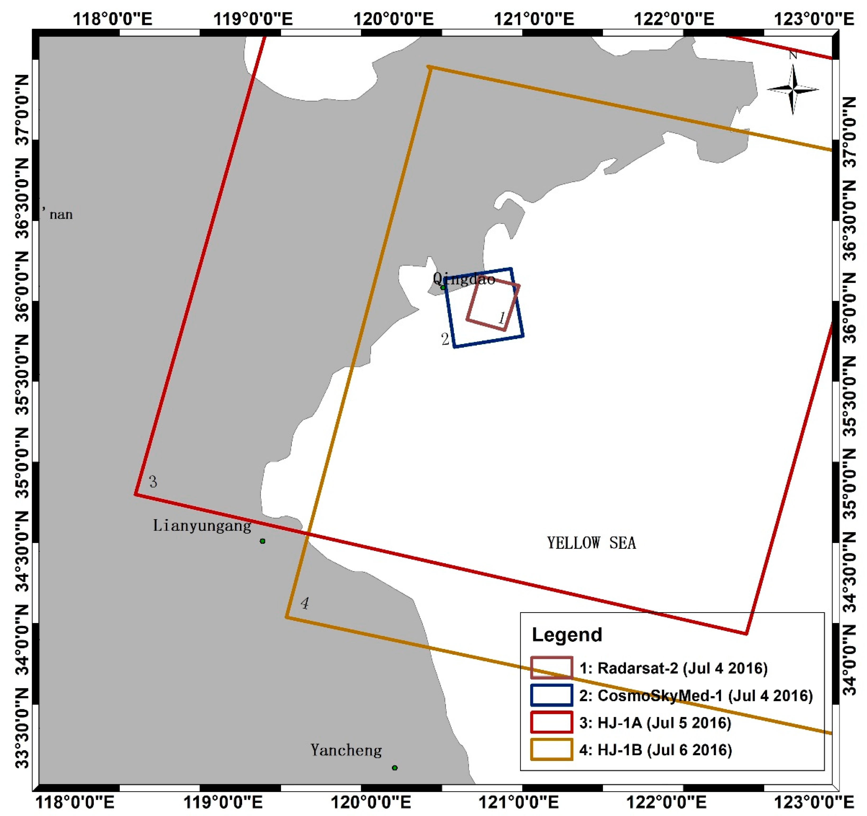
2.1. Study Area

The southern Yellow Sea, which is one of the three marginal seas of China and is dominated by east-Asian Monsoons [8,21], is the study area in this research (the black square in the overlaid graph of Figure 1). The Subei Shoal, which is located in the nearshore zone of southern Yellow Sea and is the primary aquaculture region of the Porphyra yezoensis in China, ranging from the Yangtze River delta north up to the Sheyang River, was verified to be the origin of MABs in the Yellow Sea of China [11,23]. The floating macroalgae were discarded into the nearshore area of the southern Yellow Sea every spring, resulting in the macro green tides blooming in these years. Regularly, the front of MABs eventually arrived at Shandong Peninsula in summer, driven by the currents and sea winds of the southern Yellow Sea of China, according to the results of remote sensing monitoring, model prediction, and macroalgae samples analyses [31,33,46]. Thus, the southern Yellow Sea of China was decided to be the research area to investigate the characteristics of MABs in remotely-sensed images. In July of 2016, when the macroalgae broke out in the study area, SAR images with different wave bands (C and X band) and HJ-1 series satellite CCD images were selected to synergistically retrieve instinctive parameters of MABs.

2.2. SAR Images

SAR satellites have become enriched and diversified in the last two decades because active radar sensors could acquire remote sensing images in cloudy or rainy conditions, despite the absence of daylight [57,58]. The frequency of radar system would preliminarily determine the visualization and applicability of SAR images [59,60,61]. In addition, the polarizations were also critical factors to be considered, because radar polarimetry can be used for the discrimination between different types of biomasses on the ocean and land surface of the earth [43,48,62,63,64].

Two SAR images in C and X band were collected off the south coast of Qingdao, Shandong province, which were taken by RADARSAT-2 (C band, HH/HV/VH/VV polarizations, with spatial resolution of 8 m, outlined by square #1 in Figure 1) and Cosmo-SkyMed-1 (X band, HH/VV polarizations, with spatial resolution of 15 m, outlined by square #2 in Figure 1) satellite, respectively.

The SAR images were preprocessed by Sentinel Application Platform (SNAP, Version 3.0) software provided by the European Space Agency (ESA) (http://step.esa.int/main/toolboxes/snap/ (accessed on 16 March 2023)). Firstly, SAR images of level 1 product (in single look complex type) were calibrated, i.e., all pixel values of SAR images engaged were transformed to the Normalized Radar Cross Section (NRCS) from complex. Next, the calibrated SAR images were ellipsoid-corrected and resampled to map projection images by using the ’Average Height Range-Doppler’ method in SNAP. Finally, post-processing steps were implemented such as speckle filtering, polarimetric parameters computation, etc., in the software platform.

2.3. Optical Images

In this investigation, we acquired HJ-1A (5 July) and HJ-1B (6 July) multi-spectral images to trace MABs on the Yellow Sea of China, along with SAR images. Firstly, HJ-1 series satellite images were downloaded from the website of China Centre for Resources Data and Application (https://data.cresda.cn/ (accessed on 16 March 2023)). Next, HJ-1A/B images were calibrated to radiance images and were atmospherically corrected to reflectance images by using Radiometric Calibration and FLAASH modules of ENVI5.3 software by Harris Corporation in Melbourne, Florida, USA, respectively. Finally, HJ-1A/B images were processed to pseudo-colored images and NDVI images, and then were registered to SAR images engaged in this investigation.

A summary of remotely-sensed images used in this research are listed below. Please refer to

Table 1. Specifications of remote sensing data engaged in the investigation.

Image Acquiring Time	Satellite Platform (Sensor)	Wave Band	Polarization (for SAR Image Only)	Spatial Resolution (m)	Swath (km)
4 July 2016 21:46:04 UTC	Cosmo-SkyMed-1 (SAR)	X	HH/VV	15	45
4 July 2016 22:07:08 UTC	Radarsat-2 (SAR)	C	HH/HV/VV/VH	8	25
5 July 2016 02:20:54 UTC	HJ-1A (CCD)	Visible/Infrared	-	30	400
6 July 2016 02:12:15 UTC	HJ-1B (CCD)	Visible/Infrared	-	30	400

for details.

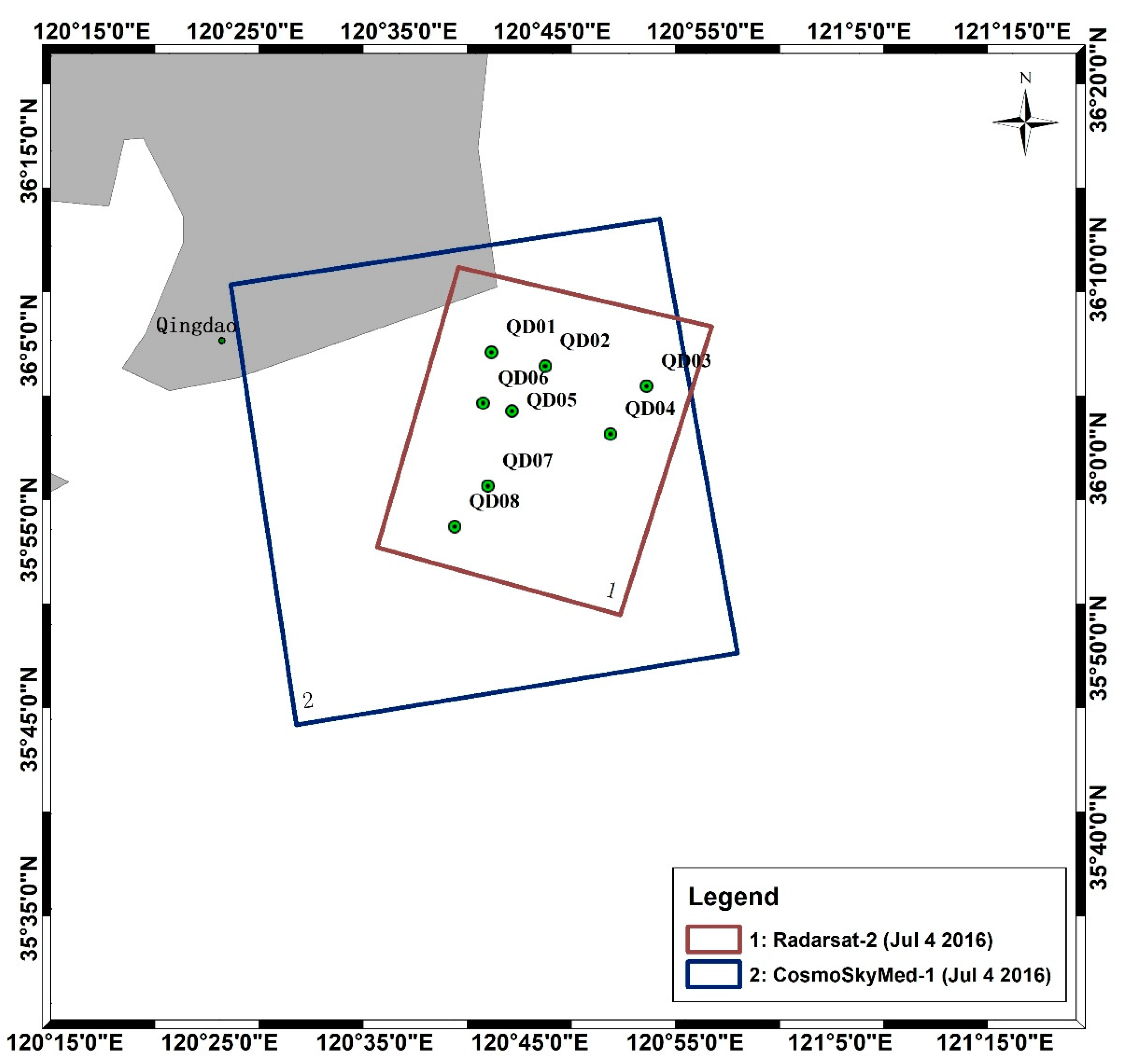
2.4. Synchronization Campaign Experiment

The on-site cruise experiment was conducted beginning at 22:46 (UTC) 4 July 2016, about 1 h later than the Radarsat-2 C band quad-polarized SAR image was acquired (22:07 UTC 4 July 2016, #1 in Figure 2), and the Cosmo-SkyMed-1 X band dual-polarized SAR image (21:46 UTC 4 July 2016, #2 in Figure 2) was taken. This synchronization campaign experiment was implemented to verify the informative parameters that were identified and retrieved from the consecutive captured SAR images and CCD imageries with as few variations of MABs as possible.

As the area (about 625 km²) of Radarsat-2 image is covered by all of the other images engaged in this research, all eight sampling stations in this investigation were set inside square #1 (see Figure 2). The sampling spots were coded in accordance with the time sequence at which the cruise arrived, and they were assigned separately from each other so that more diversified samples of MABs could be acquired. In addition, a square of 1 m × 1 m (see Figure 3) was made as the sampling tool to ensure the green algae sampled covering unit area of 1 m² on the sea surface. In the progress of the on-site experiment, when the cruise was close to a predicted sampling spot, the crew members would choose uniform and representative green algae patches to take, recording the time of sampling, the coordinates of the station, etc. For each Enteromorpha prolifera sample gathered, analysts would first discriminate its genus and then take out the excessive water for 2 min with a dryer, finally recording its weight as the wet biomass of this sample. Details about all eight samples are recorded in

Table 2. The ground-measured features of macroalgae on the Yellow Sea of China in the synchronized experiment.

Number of Sampling Station	Time of Sampling	Latitude (N)	Longitude (E)	Color of Sample	Genus Identified	Wet Biomass (kg/m2)
QD01	4 July 2016 22:56:48UTC	36°05′01.7″	120°41′32.2″	Green-Yellow	Ulva prolifera	2.2
QD02	4 July 2016 23:12:27UTC	36°04′22.0″	120°45′03.2″	Green-Yellow	Ulva prolifera	4.3
QD03	4 July 2016 23:33:45UTC	36°03′24.8″	120°51′40.1″	Green-Yellow	Ulva prolifera	1.9
QD04	4 July 2016 23:49:55UTC	36°00′50.4″	120°49′23.2″	Green-Yellow	Ulva prolifera	1.65
QD05	5 July 2016 00:07:42UTC	36°01′56.6″	120°42′57.1″	Green-Yellow	Ulva prolifera	0.95
QD06	5 July 2016 00:19:04UTC	36°02′19.5″	120°41′05.3″	Green-Yellow	Ulva prolifera	1.05
QD07	5 July 2016 00:40:23UTC	35°57′57.3″	120°41′31.2″	Green-Yellow	Ulva prolifera	1.15
QD08	5 July 2016 00:53:45UTC	35°55′46.0″	120°39′25.3″	Green-Yellow	Ulva prolifera	1.5

as references.

3. Experiment and Results

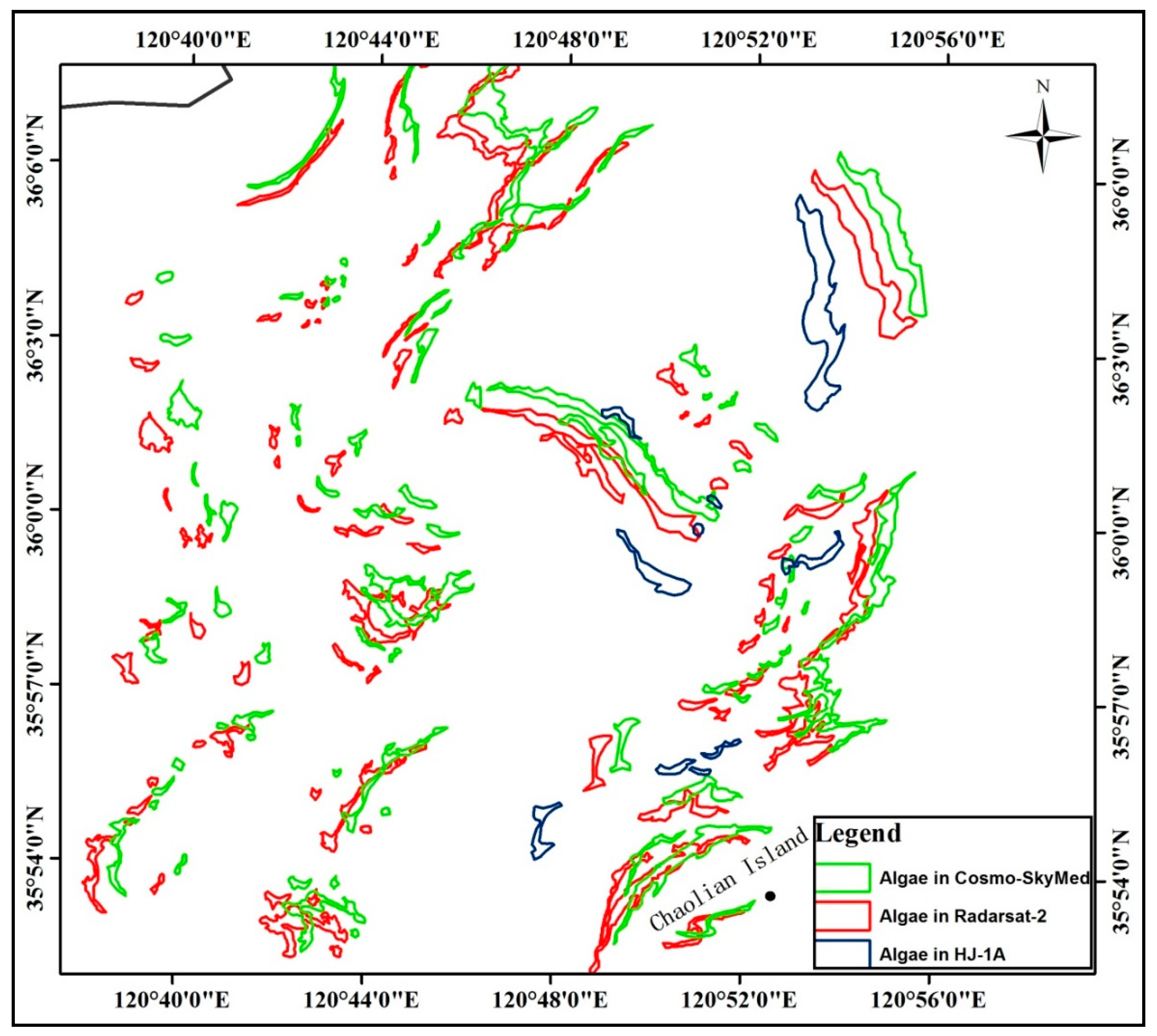
3.1. Tracing MABs by Diversified Time Series Images

One of the critical issues when it comes to monitoring and countermeasures in terms of marine hazards is to identify the pollutants on the sea surface and update their trails timely. According to the recent research, spectrometers with middle-high resolution such as Landsat-7/ETM+, Landsat-8/OLI, HJ-1/CCD, etc., had been successfully mapping the blooms of green tide off the east coast of China [8,65]. In addition, SAR has proved to be a vital complementary tool available, especially when optical instruments fail to serve in the presence of many heavy clouds upon the marine surface. As most of the wavelengths of spaceborne SAR are between 3 cm and 30 cm (corresponding to frequency bands of X, C, S, and L), SAR images are suitable for the detection of macroalgae on the sea surface, whose roughness is in the order of centimeters, no matter if it is cloudy or dark. These advantages of SAR remote sensing enrich the data sources that are engaged in the monitoring of marine pollution accidents.

Figure 4 shows massive green algae imaged by both SAR and multi-spectral images in the Yellow Sea of China, which were close to Shandong province in early July of 2016. The paired SAR images (Figure 4a,b) outlined the macroalgae on the sea surface as morphologically alike because the time between these two SAR images acquired was 21 min. The other image pair of spectral features (Figure 4c,d), processed from HJ-1A and HJ-1B CCD data, can be used to discriminate green algae from open water according to their essential discrepancy in reflectance of both near-infrared and green. It is hard to identify every green algae pair in Figure 4c,d, however, as over half of the area in Figure 4c was covered by clouds and the time delay between these two images was about 1 day.

The shape-varied characteristic of green macroalgae patches floating on the sea surface is revealed by the time series remote sensing images in Figure 4, which would significantly decrease the effectiveness and applicability of synergistic remotely-sensed images in marine disaster monitoring. Both wind and sea current stress are basically dominant driven forces in the movement of pollutants on the sea surface [33,66,67]. Owing to the green tide that initially results from the growth and connection of a large amount of macroalgae patches, it is essential to investigate the effect of air blow and sea water movement on the trajectory of macroalgae. We interpreted and outlined the macroalgae stripes by analyzing three remote sensing images (Figure 4a–c), of which the imaging start time intervals were short enough, such that the same green algae in different remote sensing images can be labeled and the effects of driven force on them can be researched in a coordinated system (see Figure 5).

To investigate the movement of floating green algae repelled by the wind force over the sea surface, the European Centre for Medium-Range Weather Forecasts (ECMWF) reanalysis data and ERA-Interim were engaged (http://www.ecmwf.int (accessed on 16 March 2023)), which were assimilated by meteorological observations, high-resolution satellite data sets, etc. [68]. On the other hand, the real-time numerical forecast data for sea current (http://marine.copernicus.eu (accessed on 16 March 2023)), provided by the COPERNICUS Marine Environment Monitoring Service of EU, were used to analyze its impact on the green algae floating on the sea surface. As the reanalyzed wind stress data products were sampled every 6 h, the data at 00:00:00 UTC 5 July 2016 were selected, which were close to the period of imaging time (from 21:46:04 UTC 4 July 2016 to 02:20:54 UTC 5 July 2016 in this study). The wind speed was 19.8 km/h and the wind direction was 235° (SW). The current vectors from the Global Ocean Physics Analysis and Forecast products, however, were sampled every 1 h. Considering the current data ranging from 21:30:00 UTC 4 July 2016 to 02:30:00 UTC 5 July 2016, we found that the current speed of sea water, within the extent of Figure 5, gently varied between 0.08 m/s and 0.1 m/s, with a stable eastward current direction in this time period of 5 h. It can be seen from Figure 5 that green algae patches were accordingly moving along the direction of dominant southwestwards (235°) wind over the sea surface in that period of time (about 4~5 h). Moreover, the weak nearshore sea current impacted less on the drift direction of macroalgae than mid-low wind force, 10 m above the marine surface. Figure 6 delineates the scatterplot of the floating distance versus observing time of green algae patches on the sea surface. The start time (0 h) is set at the time when Cosmo-SkyMed satellite image was acquired. Because the time when Radarsat-2 satellite flew over the research region was 0.34 h later than Cosmo-SkyMed, the observation time of Radarsat-2 image was plotted at 0.34 h in x-axis, followed by scattered spots from HJ-1A which were plotted at 4.2 h. The slope coefficient (0.4812 km/h) of the linear regression formula in Figure 6 was then considered as the speed at which green algae moved on the sea surface mainly driven by wind stress. In this case, the macroalgae moved at a speed of as much as 2.4% of the wind speed on the sea surface, which agrees with previous investigations [33,69], considering the higher moving speed (up to 2.94 km/h) of macroalgae might be applied. Taking the observation at 0.34 h solely into account, the proportion (the fraction green algae drifting speed divided by wind speed) would increase to about 15%.

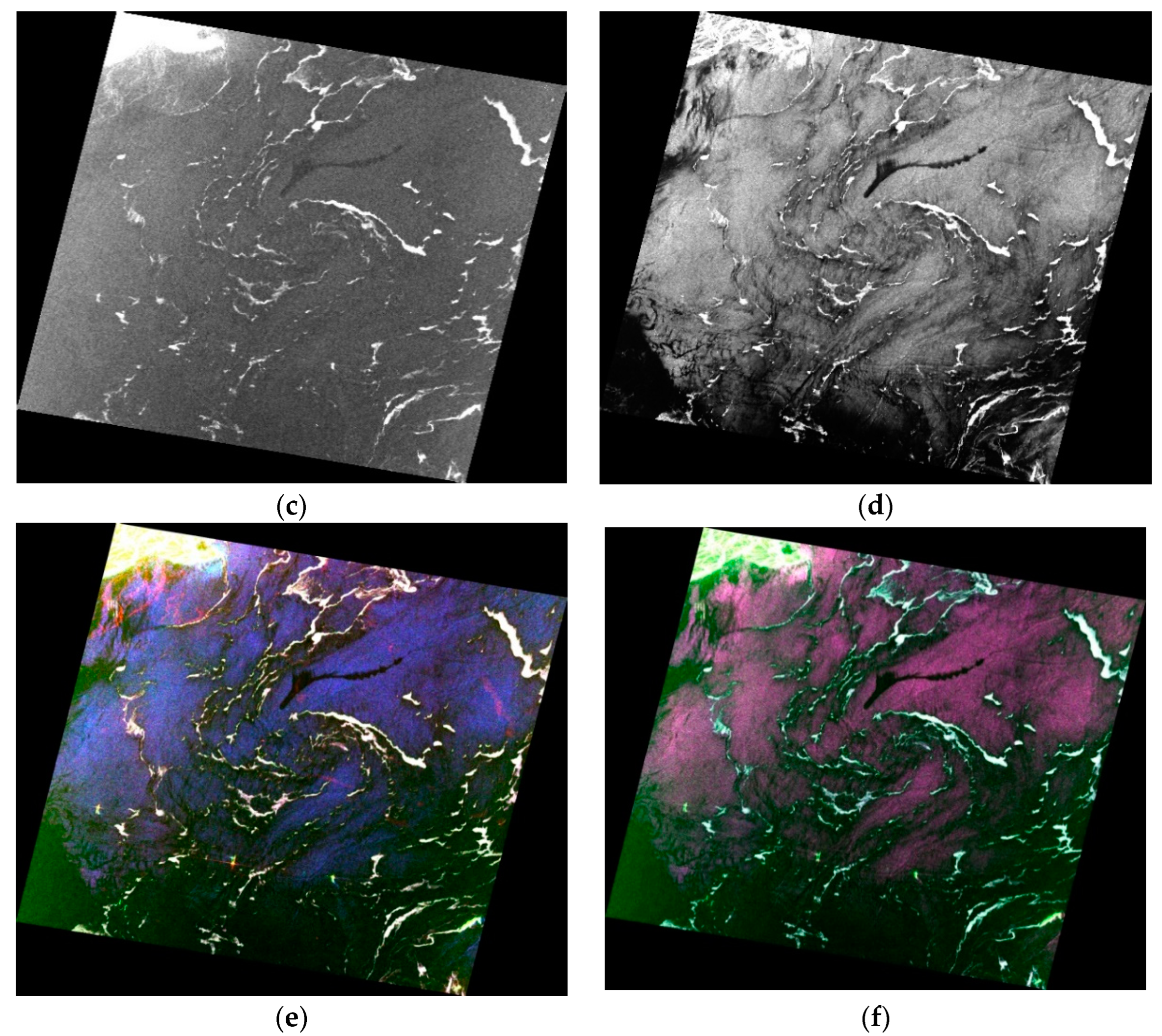
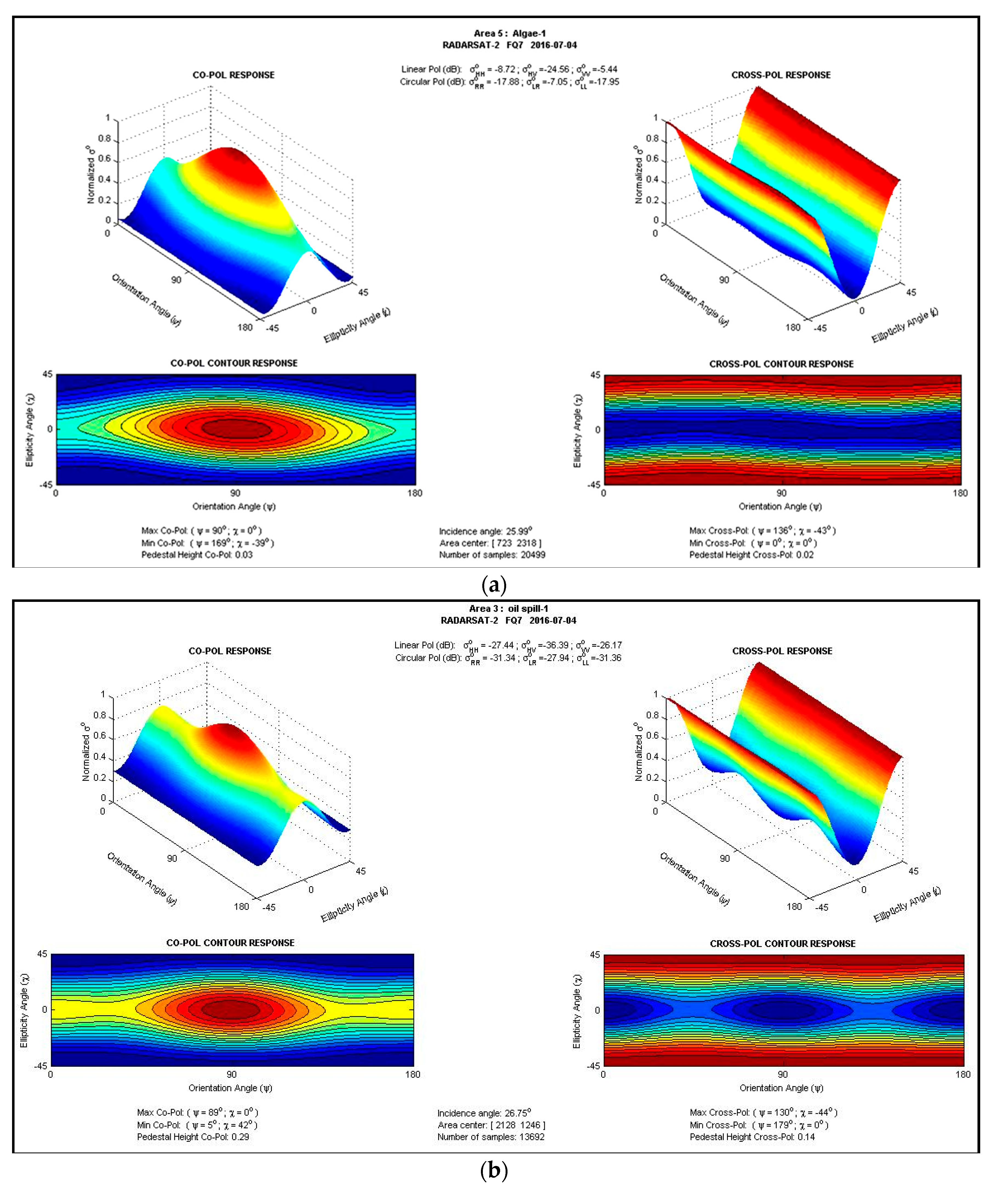
3.2. Features of Macroalgae versus Oil Spills in SAR Image

It is well known that polarimetric SAR records the response of targets on the earth by a complex scattering matrix:

$$\mathrm{S}=\left[\begin{array}{cc}{\mathrm{S}}_{\mathrm{HH}}& {\mathrm{S}}_{\mathrm{HV}}\\ {\mathrm{S}}_{\mathrm{VH}}& {\mathrm{S}}_{\mathrm{VV}}\end{array}\right]$$

(1)

where S represents the complex scattering matrix for an individual pixel in a full polarized SAR image, wherein ${\mathrm{S}}_{\mathrm{HH}}$ and ${\mathrm{S}}_{\mathrm{VV}}$ correspond to the co-polarization complex returns, and ${\mathrm{S}}_{\mathrm{HV}}$ and ${\mathrm{S}}_{\mathrm{VH}}$ correspond to the cross-polarization terms, respectively. Moreover, either the coherence $\langle \left[{\mathrm{T}}_3\right]\rangle$ or covariance $\langle \left[{\mathrm{C}}_3\right]\rangle$ matrix is essential in terms of polarimetric target decomposition instead of S when natural objects (also known as distributed targets) are investigated, which can be mathematically written as:

$$\langle \left[{\mathrm{T}}_3\right]\rangle =\frac{1}{2}\left[\begin{array}{ccc}{\langle \left|{\mathrm{S}}_{\mathrm{HH}}+{\mathrm{S}}_{\mathrm{VV}}\right|\rangle }^2& \langle \left({\mathrm{S}}_{\mathrm{HH}}+{\mathrm{S}}_{\mathrm{VV}}\right){\left({\mathrm{S}}_{\mathrm{HH}}-{\mathrm{S}}_{\mathrm{VV}}\right)}^{*}\rangle & 2\langle \left({\mathrm{S}}_{\mathrm{HH}}+{\mathrm{S}}_{\mathrm{VV}}\right){\mathrm{S}}_{\mathrm{HV}}{}^{*}\rangle \\ \langle \left({\mathrm{S}}_{\mathrm{HH}}-{\mathrm{S}}_{\mathrm{VV}}\right){\left({\mathrm{S}}_{\mathrm{HH}}+{\mathrm{S}}_{\mathrm{VV}}\right)}^{*}\rangle & {\langle \left|{\mathrm{S}}_{\mathrm{HH}}-{\mathrm{S}}_{\mathrm{VV}}\right|\rangle }^2& 2\langle \left({\mathrm{S}}_{\mathrm{HH}}-{\mathrm{S}}_{\mathrm{VV}}\right){\mathrm{S}}_{\mathrm{HV}}{}^{*}\rangle \\ 2\langle {\mathrm{S}}_{\mathrm{HV}}{\left({\mathrm{S}}_{\mathrm{HH}}+{\mathrm{S}}_{\mathrm{VV}}\right)}^{*}\rangle & 2\langle {\mathrm{S}}_{\mathrm{HV}}{\left({\mathrm{S}}_{\mathrm{HH}}-{\mathrm{S}}_{\mathrm{VV}}\right)}^{*}\rangle & 4{\langle \left|{\mathrm{S}}_{\mathrm{HV}}\right|}^2\rangle \end{array}\right]$$

(2)

and

$$\langle \left[{\mathrm{C}}_3\right]\rangle =\left[\begin{array}{ccc}{\langle \left|{\mathrm{S}}_{\mathrm{HH}}\right|}^2\rangle & \sqrt{2}\langle {\mathrm{S}}_{\mathrm{HH}}{\mathrm{S}}_{\mathrm{HV}}{}^{*}\rangle & \langle {\mathrm{S}}_{\mathrm{HH}}{\mathrm{S}}_{\mathrm{VV}}{}^{*}\rangle \\ \sqrt{2}\langle {\mathrm{S}}_{\mathrm{HV}}{\mathrm{S}}_{\mathrm{HH}}{}^{*}\rangle & 2{\langle \left|{\mathrm{S}}_{\mathrm{HV}}\right|}^2\rangle & \sqrt{2}\langle {\mathrm{S}}_{\mathrm{HV}}{\mathrm{S}}_{\mathrm{VV}}{}^{*}\rangle \\ \langle {\mathrm{S}}_{\mathrm{VV}}{\mathrm{S}}_{\mathrm{HH}}{}^{*}\rangle & \sqrt{2}\langle {\mathrm{S}}_{\mathrm{VV}}{\mathrm{S}}_{\mathrm{HV}}{}^{*}\rangle & {\langle \left|{\mathrm{S}}_{\mathrm{VV}}\right|}^2\rangle \end{array}\right]$$

(3)

where $\langle ·\rangle$ denotes the ensemble average operator, which is necessary for the processing of SAR image data due to the presence of coherence noise, and ${}^{*}$ represents the complex conjunction.

Both $\langle \left[{\mathrm{T}}_3\right]\rangle$ and $\langle \left[{\mathrm{C}}_3\right]\rangle$ are positive semidefinite Hermitian matrices, and are connected by the total power backscattered [70]:

$$\mathrm{Span}=\mathrm{Tr}\left(\langle \left[{\mathrm{T}}_3\right]\rangle \right)=\mathrm{Tr}\left(\langle \left[{\mathrm{C}}_3\right]\rangle \right)$$

(4)

where $\mathrm{Tr}(\langle M\rangle )$ denotes the trace of the Matrix M, and can be represented as follows:

$$\mathrm{Tr}\left(\langle \left[{\mathrm{T}}_3\right]\rangle \right)=\frac{1}{2}\left({\langle \left|{\mathrm{S}}_{\mathrm{HH}}+{\mathrm{S}}_{\mathrm{VV}}\right|}^2\rangle +{\langle \left|{\mathrm{S}}_{\mathrm{HH}}-{\mathrm{S}}_{\mathrm{VV}}\right|}^2\rangle +4{\langle \left|{\mathrm{S}}_{\mathrm{HV}}\right|}^2\rangle \right)$$

(5)

$$\mathrm{Tr}\left(\langle \left[{\mathrm{C}}_3\right]\rangle \right)={\langle \left|{\mathrm{S}}_{\mathrm{HH}}\right|}^2\rangle +2{\langle \left|{\mathrm{S}}_{\mathrm{HV}}\right|}^2\rangle +{\langle \left|{\mathrm{S}}_{\mathrm{VV}}\right|}^2\rangle$$

(6)

According to the theorem of ‘average’ scattering mechanism [71], the real diagonal elements of the coherence matrix $\langle \left[{\mathrm{T}}_3\right]\rangle$ can be used to evaluate the contribution of three fundamental scattering schemes, i.e., surface scattering, dihedral scattering, and volume scattering. For the covariance matrix $\langle \left[{\mathrm{C}}_3\right]\rangle$, however, the real diagonal elements are vitally significant because the specific response backscattered from targets can be compared between co-polarization and cross-polarization terms, and the depolarized effects are thus able to be investigated [48,59]. Figure 7 exhibits the multi-polluted ocean image of the Yellow Sea of China, which was taken by the Radarsat-2 full-polarized SAR and is investigated in this research. The prevalent scattering mechanism of green algae, open water, and oil spill were overall analyzed, respectively, by using the polarimetric parameters mentioned above. See the figure captions for details.

Quantitatively, the overall polarimetric signatures of targets can be delineated by normalized ${\mathsf{\sigma }}_0$ of co- and cross-polarization [72,73]. In this investigation, the polarimetric characteristics of three typical objects in SAR image, i.e., macroalgae, oil spill, and open water, were further analyzed using Polarimetric Workstation Software Version 5.4 software, which was developed by the Canada Centre for Remote Sensing (CCRS) (see Figure 8 for reference).

The green algae, which look like vegetables floating on the sea surface, showed as single bounce scattering (Figure 8a). To be specific, for the green algae, the maximum response (−5.44 dB) of co-pol happened when VV polarization ($\mathsf{\psi }=90°, \mathsf{\chi }=0°$) was applied, whereas the minimum one (−17.88 dB) happened when RR polarization ($\mathsf{\psi }=169°, \mathsf{\chi }=-39°$) was applied. On the other hand, the maximum response (−7.05 dB) of cross-pol occurred when LR polarization ($\mathsf{\psi }=136°, \mathsf{\chi }=-43°$) was applied, whereas the minimum one (−24.56 dB) occurred when HV polarization ($\mathsf{\psi }=0°, \mathsf{\chi }=0°$) was applied (see Figure 8a for reference). This implies that circular polarized SAR in LR polarization (i.e., right circular polarization transmitted and left circular polarization received) is supposed to be a candidate as a novel sensor, considering a mission of global algae monitoring and biomass of macroalgae evaluation around the world.

Moreover, the polarimetric signatures of oil spill (Figure 8b) and open water (Figure 8c), similar to the green algae (Figure 8a), are interpreted as $\mathrm{VV}>\mathrm{HH}\gg \mathrm{RR}/\mathrm{LL}$ (for co-pol) and $\mathrm{VH}/\mathrm{HV}\ll \mathrm{LR}/\mathrm{RL}$ (for cross-pol), corresponding to the typical surface scattering [74].

The NRCS, however, identically varied among three types of objects on the sea surface according to Figure 8. For comparison, we summarized the NRCS of macroalgae, oil spill, and open water in six polarimetric channels of SAR images in Figure 9. It can be concluded that VV or HH are optimal co-polarization combinations to discriminate between the pollutant (either macroalgae or oil spill) and the surrounding sea surface in a polarimetric SAR image. LL and RR, on the contrary, are not able to distinguish the oil spill from the background sea correctly because they are ‘look-alikes’ in LL/RR SAR image, which might be produced by the compact polarimetric (CP) mode SAR data [75,76] or the PALSAR-2 (the Phased Array type L-band Synthetic Aperture Radar) onboard ALOS-2 (the Japanese Advanced Land Observing Satellite), for instance. In addition, the LR polarimetric channel is the only cross-polarization combination candidate for the discrimination between macroalgae, oil spill, and open water because of the ineffectiveness of linear cross-polarization, i.e., HV or VH according to Figure 9.

3.3. Floating Algae Index of Polarimetric SAR

The macroalgae bloom (when eutrophic environment is applied, and abundant sunlight is provided) results in the deterioration of marine ecosystem and the interference of marine transportation. It is vital to identify green algae quantitatively by means of remote sensing technology to evaluate this kind of ocean disaster effectively. Polarimetric SAR images are widely used in target detection and natural hazards assessment [52,77] due to their capability of the characteristic measurements of targets such as moisture content, surface roughness, etc.

In this paper, a Floating Algae Index by Polarimetric SAR image (FAIPS) was proposed as follows:

$$\mathrm{FAIPS}={\left|{\mathrm{S}}_{\mathrm{HH}}\right|}^2+2{\left|{\mathrm{S}}_{\mathrm{HV}}\right|}^2+{\left|{\mathrm{S}}_{\mathrm{VV}}\right|}^2$$

(7)

where ${\mathrm{S}}_{\mathrm{HH}},{ \mathrm{S}}_{\mathrm{HV},}{ \mathrm{and} \mathrm{S}}_{\mathrm{VV}}$ were the elements of S matrix in polarimetric SAR data, which are defined in Equation (1). From Equation (7), it can be concluded that FAIPS is determined by NRCS of all of four polarimetric channels.

The features of macroalgae samples collected in eight sample stations are summarized in

Table 3. The features of macroalgae that were sampled in this investigation.

Sample Station	Wet Biomass per Area (kg/m2)	Time Delay from Radarsat-2 Polarimetric SAR Image Acquisition Time to the Sample Time of the Station (min)	$\left|{\mathbf{S}}_{\mathbf{H}\mathbf{H}}\right|$	$\left|{\mathbf{S}}_{\mathbf{H}\mathbf{V}}\right|$	$\left|{\mathbf{S}}_{\mathbf{V}\mathbf{V}}\right|$	$\mathbf{F}\mathbf{A}\mathbf{I}\mathbf{P}\mathbf{S}$
QD01	2.2	50	0.1960	0.0343	0.2789	0.1186
QD02	4.3	65	0.2612	0.0435	0.3848	0.2201
QD03	1.9	87	0.1714	0.0271	0.2484	0.0924
QD04	1.65	103	0.1849	0.0310	0.2642	0.1060
QD05	0.95	121	0.1861	0.0319	0.2656	0.1072
QD06	1.05	132	0.1867	0.0301	0.2735	0.1115
QD07	1.15	153	0.1574	0.0265	0.2240	0.0763
QD08	1.5	167	0.2018	0.0344	0.2912	0.1279

. It is worth noticing that the time when the first sample of macroalgae was collected in QD01 sample station, which is close to Shandong Peninsula (see Figure 2), was delayed for about 50 min since the Radasat-2 Quad-Polarization SAR image was acquired (referring to Figure 1), from which $\langle \left|{\mathrm{S}}_{\mathrm{HH}}\right|\rangle$, $\langle \left|{\mathrm{S}}_{\mathrm{HV}}\right|\rangle ,$ and $\langle \left|{\mathrm{S}}_{\mathrm{VV}}\right|\rangle$ were statistically computed. Moreover, it can be seen from Table 3 that the maximum (0.0435) of cross-polarization response, i.e., $\left|{\mathrm{S}}_{\mathrm{HV}}\right|$ occurred when the maximum of wet biomass of macroalgae sample (QD02) was observed, which was two times greater than that of the lower biomass of macroalgae sample—QD07, for example. This demonstrated that the hybrid scattering happened when the sea surface was covered by macroalgae of a higher biomass.

3.4. Floating Algae Biomass Evaluation Model

Figure 10 shows an exponential relationship between FAIPS and wet biomass per area (kg/m²) of macroalgae sampled on the Yellow Sea of China in this investigation, on 5 July 2016.

4. Discussions

4.1. Challenge of the Synchronization Experiment

We coordinated the satellite images acquisition and ground truth verification to implement a synchronization experiment off the east coast of Qingdao, China, on 5 July 2016 in this investigation. Our team arrived at QD01 station and sampled the Ulva prolifera at 22:56 UTC 4 July 2006, when about 50 minutes after the first polarimetric SAR image (RadarSAT-2) was acquired (22:07 UTC 4 July 2006), or 70 minutes after the Cosmo-SkyMed SAR image was acquired (21:46 UTC 4 July 2006). One of the challenges in this synchronization experiment was to match the sample spot (referring to the coordinates recorded by the GPS receiver that the team member carried) with the SAR image. Because of the time delay of 50 min, it is probably tough to find the corresponding sample spot (quite close to a macroalgae patch) on the SAR image. Firstly, we labeled the point of the first sample station, for example, on the Radarsat-2 image in accordance with the coordinates recorded. Following that, we moved the point to a spot 1.2 km away, northeastwards. This is because, according to the regress model (Figure 6), the macroalgae patches would have traveled around 1.2 km (at averaged speed of 0.4812 km/h), southwestwards (Figure 5), in 50 min. In this way, we were usually able to locate the Ulva prolifera patch on RadarSAT-2 polarimetric SAR image, where the ground truth team sampled the algae. Finally, we statistically collected and set the NRCS (i.e., ${\langle \left|{\mathrm{S}}_{\mathrm{HH}}\right|}^2\rangle$, ${\langle \left|{\mathrm{S}}_{\mathrm{HV}}\right|}^2\rangle$ and ${\langle \left|{\mathrm{S}}_{\mathrm{VV}}\right|}^2\rangle$) of the patch on SAR image as the feature values for the sample algae in Table 3.

In addition, the influence of clouds on optical images is another challenge in this synchronization experiment. Because of the cloud, most of the macroalgae on HJ-1A CCD image (02:20:54 UTC 5 July 2016) were not captured (see Figure 4c), resulting in fewer blue patches in Figure 5. This might deteriorate the predicting accuracy of the regression model (Figure 6).

Last but not least, we selected a much bigger area of patches on SAR image to abstract the features of algae samples, to reduce the accidental error produce by the sampling procedure. This quantification, however, might induce additional uncertainty concerning NRCS assessment because of the inhomogeneity of the floating algae samples on the sea surface. The methodology of feature abstraction from the SAR images proposed in this paper can be taken as a trade-off.

4.2. Macroalgae Biomass Assessment by Means of Remote Sensing Images

The regression equation (in Figure 10) proposed in this investigation can be used in the evaluation of the biomass of Ulva prolifera macroalgae on the sea surface. Hu et al. implemented an experiment in laboratories to measure the wet and dry biomass per area of Ulva. prolifera and to establish an exponential model, relating the biomass per area to the reflectance of macroalgae on MODIS images in 2017 [78]. Moreover, Xiao et al. found there were significant exponential relationships between the biomass per area of Ulva prolifera and EVI (Enhanced Vegetation Index), with R² > 0.9 and the average percentage deviation (APD) ≈ 20%, for the simulated MODIS $R_{rs}$ (the reflectance measured in situ experiment of water tank in 2019, by a FieldSpec4 ASD spectrometer with 1 nm resolution from 350 to 2500 nm) [79]. For the simulated MODIS $R_{rc}$ (Rayleigh-corrected reflectance) and $R_{toa}$ (top-of-atmosphere reflectance) under various aerosol optical depths at 550 nm (${\tau }_{550}$), there were exponential relationships between the biomass per area and various indices (e.g., RVI, NDVI, FAI, KOSC, and OSABI). The coefficients of the fitting formulas, however, were significantly affected by the AOT (Aerosol Optical Thickness).

The FAIPS proposed in this paper is hopefully a polarimetric SAR image-based index that can be engaged in the identification of the floating Ulva prolifera macroalgae on the sea surface, which is hardly influenced by the atmosphere effects and the lack of daylight. Considering the absence of polarimetric SAR data, the dual polarized (HH/HV or VV/VH) SAR image can also be used because of the co-polarization channel (HH or VV), which is shown as a similar response to the macroalgae samples according to Figure 9.

Considering the FAIPS-based exponential regression model proposed in this investigation (Figure 10),

$$y=0.5613e^{8.9082x}$$

(8)

where x denotes the FAIPS index from the polarimetric SAR image and y denotes the predicted wet biomass per area (in kg/m²) of macroalgae on the sea surface. We were able to evaluate that the total wet biomass of macroalgae on the Yellow Sea of China was around 28–43 kilotons, according to Equation (8), by using the Radarsat-2 polarimetric SAR image taken on 4 July 2016 (see Table 1). This assessment was in good agreement with the evaluated result (37.3 kilotons) by using MODIS data taken on 2 July 2016 in the study area of this investigation [79,80].

5. Conclusions

Remote sensing evaluation of biomass for the macroalgae on the sea surface has been reported by using satellite images such as MODIS, Landsat, etc., in recent years, based on the spectral reflectance or feature indexes such as EVI, NDVI, etc. In this paper, we implemented a synchronization experiment to coordinate the satellite image acquisition and ground truth verification to obtain the relationship between wet biomass of macroalgae and its features on polarimetric SAR images. Following that, the FAIPS index-based exponential regression equation was proposed to evaluate the macroalgae biomass of Ulva prolifera in the Yellow Sea of China by using polarimetric SAR images. The algorithm proposed in this paper can be applied in the monitoring and biomass assessment of macroalgae blooms when medium-high resolution polarimetric SAR images are available, regardless of daylight and cloud coverage over the sea surface.

References

1. Gade, M.; Rud, O.; Barale, V.; Snaith, H.M.; Jolly, G.W. Multisensor Studies of Oceanic Phaenomena in European Marginal Waters: Algae Blooms in the Baltic Sea and a River Plume in the Mediterranean. Eur. Space Agency 2000, 114, 1844–1855. [Google Scholar]
2. Garcia, R.A.; Fearns, P.; Keesing, J.K.; Liu, D. Quantification of Floating Macroalgae Blooms Using the Scaled Algae Index. J. Geophys. Res. Ocean. 2013, 118, 26–42. [Google Scholar] [CrossRef] [Green Version]
3. Keesing, J.K.; Liu, D.; Fearns, P.; Garcia, R. Inter- and Intra-Annual Patterns of Ulva Prolifera Green Tides in the Yellow Sea during 2007–2009, Their Origin and Relationship to the Expansion of Coastal Seaweed Aquaculture in China. Mar. Pollut. Bull. 2011, 62, 1169–1182. [Google Scholar] [CrossRef] [PubMed]
4. Liu, Y.; Shao, Y.; Qi, X.; Tian, W.; Wen, B. Natural Marine Oil Seepage Detection and Evaluation with SAR. In Proceedings of the Sixth International Symposium on Digital Earth: Data Processing and Applications, Beijing, China, 9–12 September 2009; Volume 7841, p. 78411L. [Google Scholar] [CrossRef]
5. Liu, D.; Keesing, J.K.; Dong, Z.; Zhen, Y.; Di, B.; Shi, Y.; Fearns, P.; Shi, P. Recurrence of the World’s Largest Green-Tide in 2009 in Yellow Sea, China: Porphyra Yezoensis Aquaculture Rafts Confirmed as Nursery for Macroalgal Blooms. Mar. Pollut. Bull. 2010, 60, 1423–1432. [Google Scholar] [CrossRef] [PubMed]
6. Shi, W.; Wang, M. Green Macroalgae Blooms in the Yellow Sea during the Spring and Summer of 2008. J. Geophys. Res. Ocean. 2009, 114, 1–10. [Google Scholar] [CrossRef] [Green Version]
7. Son, S.H.; Wang, M.; Shon, J.K. Satellite Observations of Optical and Biological Properties in the Korean Dump Site of the Yellow Sea. Remote Sens. Environ. 2011, 115, 562–572. [Google Scholar] [CrossRef]
8. Xing, Q.; Hu, C. Mapping Macroalgal Blooms in the Yellow Sea and East China Sea Using HJ-1 and Landsat Data: Application of a Virtual Baseline Reflectance Height Technique. Remote Sens. Environ. 2016, 178, 113–126. [Google Scholar] [CrossRef]
9. Xu, Q.; Zhang, H.; Ju, L.; Chen, M. Interannual Variability of Ulva Prolifera Blooms in the Yellow Sea. Int. J. Remote Sens. 2014, 35, 4099–4113. [Google Scholar] [CrossRef]
10. Smetacek, V.; Zingone, A. Green and Golden Seaweed Tides on the Rise. Nature 2013, 504, 84–88. [Google Scholar] [CrossRef] [Green Version]
11. Wang, Z.; Xiao, J.; Fan, S.; Li, Y.; Liu, X.; Liu, D. Who Made the World’s Largest Green Tide in China?—An Integrated Study on the Initiation and Early Development of the Green Tide in Yellow Sea. Limnol. Oceanogr. 2015, 60, 1105–1117. [Google Scholar] [CrossRef]
12. Fan, S.; Fu, M.; Wang, Z.; Zhang, X.; Song, W.; Li, Y.; Liu, G.; Shi, X.; Wang, X.; Zhu, M. Temporal Variation of Green Macroalgal Assemblage on Porphyra Aquaculture Rafts in the Subei Shoal, China. Estuar. Coast. Shelf Sci. 2015, 163, 23–28. [Google Scholar] [CrossRef]
13. Cui, T.W.; Zhang, J.; Sun, L.E.; Jia, Y.J.; Zhao, W.; Wang, Z.L.; Meng, J.M. Satellite Monitoring of Massive Green Macroalgae Bloom (GMB): Imaging Ability Comparison of Multi-Source Data and Drifting Velocity Estimation. Int. J. Remote Sens. 2012, 33, 5513–5527. [Google Scholar] [CrossRef]
14. Liu, D.; Keesing, J.K.; He, P.; Wang, Z.; Shi, Y.; Wang, Y. The World’s Largest Macroalgal Bloom in the Yellow Sea, China: Formation and Implications. Estuar. Coast. Shelf Sci. 2013, 129, 2–10. [Google Scholar] [CrossRef]
15. Lyons, D.A.; Arvanitidis, C.; Blight, A.J.; Chatzinikolaou, E.; Guy-Haim, T.; Kotta, J.; Orav-Kotta, H.; Queirós, A.M.; Rilov, G.; Somerfield, P.J.; et al. Macroalgal Blooms Alter Community Structure and Primary Productivity in Marine Ecosystems. Glob. Chang. Biol. 2014, 20, 2712–2724. [Google Scholar] [CrossRef]
16. Xing, Q.; Tosi, L.; Braga, F.; Gao, X.; Gao, M. Interpreting the Progressive Eutrophication behind the World’s Largest Macroalgal Blooms with Water Quality and Ocean Color Data. Nat. Hazards 2015, 78, 7–21. [Google Scholar] [CrossRef] [Green Version]
17. Xing, Q.; Hu, C.; Tang, D.; Tian, L.; Tang, S.; Wang, X.H.; Lou, M.; Gao, X. World’s Largest Macroalgal Blooms Altered Phytoplankton Biomass in Summer in the Yellow Sea: Satellite Observations. Remote Sens. 2015, 7, 12297–12313. [Google Scholar] [CrossRef] [Green Version]
18. Xing, Q.; Wu, L.; Tian, L.; Cui, T.; Li, L.; Kong, F.; Gao, X.; Wu, M. Remote Sensing of Early-Stage Green Tide in the Yellow Sea for Floating-Macroalgae Collecting Campaign. Mar. Pollut. Bull. 2018, 133, 150–156. [Google Scholar] [CrossRef]
19. Zhang, J.; Huo, Y.; Wu, H.; Yu, K.; Kim, J.K.; Yarish, C.; Qin, Y.; Liu, C.; Xu, R.; He, P. The Origin of the Ulva Macroalgal Blooms in the Yellow Sea in 2013. Mar. Pollut. Bull. 2014, 89, 276–283. [Google Scholar] [CrossRef]
20. Jin, S.; Liu, Y.; Sun, C.; Wei, X.; Li, H.; Han, Z. A Study of the Environmental Factors Influencing the Growth Phases of Ulva Prolifera in the Southern Yellow Sea, China. Mar. Pollut. Bull. 2018, 135, 1016–1025. [Google Scholar] [CrossRef]
21. Ye, N.h.; Zhang, X.w.; Mao, Y.z.; Liang, C.w.; Xu, D.; Zou, J.; Zhuang, Z.m.; Wang, Q.y. “Green Tides” Are Overwhelming the Coastline of Our Blue Planet: Taking the World’s Largest Example. Ecol. Res. 2011, 26, 477–485. [Google Scholar] [CrossRef]
22. Liu, D.; Keesing, J.K.; Xing, Q.; Shi, P. World’s Largest Macroalgal Bloom Caused by Expansion of Seaweed Aquaculture in China. Mar. Pollut. Bull. 2009, 58, 888–895. [Google Scholar] [CrossRef] [PubMed]
23. Liu, X.; Li, Y.; Wang, Z.; Zhang, Q.; Cai, X. Cruise Observation of Ulva Prolifera Bloom in the Southern Yellow Sea, China. Estuar. Coast. Shelf Sci. 2015, 163, 17–22. [Google Scholar] [CrossRef]
24. Liu, F.; Pang, S.; Chopin, T.; Gao, S.; Shan, T.; Zhao, X.; Li, J. Understanding the Recurrent Large-Scale Green Tide in the Yellow Sea: Temporal and Spatial Correlations between Multiple Geographical, Aquacultural and Biological Factors. Mar. Environ. Res. 2013, 83, 38–47. [Google Scholar] [CrossRef]
25. Son, Y.B.; Choi, B.J.; Kim, Y.H.; Park, Y.G. Tracing Floating Green Algae Blooms in the Yellow Sea and the East China Sea Using GOCI Satellite Data and Lagrangian Transport Simulations. Remote Sens. Environ. 2015, 156, 21–33. [Google Scholar] [CrossRef]
26. Shi, X.; Qi, M.; Tang, H.; Han, X. Spatial and Temporal Nutrient Variations in the Yellow Sea and Their Effects on Ulva Prolifera Blooms. Estuar. Coast. Shelf Sci. 2015, 163, 36–43. [Google Scholar] [CrossRef]
27. Song, W.; Peng, K.; Xiao, J.; Li, Y.; Wang, Z.; Liu, X.; Fu, M.; Fan, S.; Zhu, M.; Li, R. Effects of Temperature on the Germination of Green Algae Micro-Propagules in Coastal Waters of the Subei Shoal, China. Estuar. Coast. Shelf Sci. 2015, 163, 63–68. [Google Scholar] [CrossRef]
28. Xu, X. New Techniques for Radar Target Scattering Signature Measurement and Processing, 1st ed.; National Defense Industry Press of China: Beijing, China, 2017; ISBN 987-7-118-11418-8. [Google Scholar]
29. Hedley, J.; Russell, B.; Randolph, K.; Dierssen, H. A Physics-Based Method for the Remote Sensing of Seagrasses. Remote Sens. Environ. 2016, 174, 134–147. [Google Scholar] [CrossRef]
30. Lee, J.H.; Pang, I.C.; Moon, I.J.; Ryu, J.H. On Physical Factors That Controlled the Massive Green Tide Occurrence along the Southern Coast of the Shandong Peninsula in 2008: A Numerical Study Using a Particle-Tracking Experiment. J. Geophys. Res. Ocean. 2011, 116, 1–12. [Google Scholar] [CrossRef] [Green Version]
31. Pang, S.J.; Liu, F.; Shan, T.F.; Xu, N.; Zhang, Z.H.; Gao, S.Q.; Chopin, T.; Sun, S. Tracking the Algal Origin of the Ulva Bloom in the Yellow Sea by a Combination of Molecular, Morphological and Physiological Analyses. Mar. Environ. Res. 2010, 69, 207–215. [Google Scholar] [CrossRef] [Green Version]
32. Roelfsema, C.M.; Lyons, M.; Kovacs, E.M.; Maxwell, P.; Saunders, M.I.; Samper-Villarreal, J.; Phinn, S.R. Multi-Temporal Mapping of Seagrass Cover, Species and Biomass: A Semi-Automated Object Based Image Analysis Approach. Remote Sens. Environ. 2014, 150, 172–187. [Google Scholar] [CrossRef]
33. Bao, M.; Guan, W.; Yang, Y.; Cao, Z.; Chen, Q. Drifting Trajectories of Green Algae in the Western Yellow Sea during the Spring and Summer of 2012. Estuar. Coast. Shelf Sci. 2015, 163, 9–16. [Google Scholar] [CrossRef]
34. Xu, F.; Gao, Z.; Jiang, X.; Shang, W.; Ning, J.; Song, D.; Ai, J. A UAV and S2A Data-Based Estimation of the Initial Biomass of Green Algae in the South Yellow Sea. Mar. Pollut. Bull. 2018, 128, 408–414. [Google Scholar] [CrossRef] [PubMed]
35. Yuan, C.; Xiao, J.; Zhang, X.; Zhou, J.; Wang, Z. A New Assessment of the Algal Biomass of Green Tide in the Yellow Sea. Mar. Pollut. Bull. 2022, 174, 113253. [Google Scholar] [CrossRef]
36. Brisco, B.; Li, K.; Tedford, B.; Charbonneau, F.; Yun, S.; Murnaghan, K. Compact Polarimetry Assessment for Rice and Wetland Mapping. Int. J. Remote Sens. 2013, 34, 1949–1964. [Google Scholar] [CrossRef] [Green Version]
37. Hu, C.; Li, X.; Pichel, W.G.; Muller-Karger, F.E. Detection of Natural Oil Slicks in the NW Gulf of Mexico Using MODIS Imagery. Geophys. Res. Lett. 2009, 36, L01604. [Google Scholar] [CrossRef]
38. Li, X. The First Sentinel-1 SAR Image of a Typhoon. Acta Oceanol. Sin. 2015, 34, 1–2. [Google Scholar] [CrossRef]
39. Li, X.; Guo, H. Remote Sensing of the China Seas. Int. J. Remote Sens. 2014, 35, 3919–3925. [Google Scholar] [CrossRef]
40. Shao, Y.; Fan, X.; Liu, H.; Xiao, J.; Ross, S.; Brisco, B.; Brown, R.; Staples, G. Rice Monitoring and Production Estimation Using Multitemporal RADARSAT. Remote Sens. Environ. 2001, 76, 310–325. [Google Scholar] [CrossRef]
41. Nunziata, F.; Migliaccio, M.; Li, X. Sea Oil Slick Observation Using Hybrid-Polarity SAR Architecture. IEEE J. Ocean. Eng. 2015, 40, 426–440. [Google Scholar] [CrossRef]
42. Tian, W.; Bian, X.; Shao, Y.; Zhang, Z. On the Detection of Oil Spill with China’s HJ-1C SAR Image. Aquat. Procedia 2015, 3, 144–150. [Google Scholar] [CrossRef]
43. Tian, W.; Shao, Y.; Yuan, J.; Wang, S.; Liu, Y. An Experiment for Oil Spill Recognition Using RADARSAT-2 Image. Int. Geosci. Remote Sens. Symp. 2010, 2761–2764. [Google Scholar] [CrossRef]
44. Zhang, B.; Perrie, W.; Li, X.; Pichel, W.G. Mapping Sea Surface Oil Slicks Using RADARSAT-2 Quad-Polarization SAR Image. Geophys. Res. Lett. 2011, 38, L10602. [Google Scholar] [CrossRef] [Green Version]
45. Aslan, A.; Rahman, A.F.; Warren, M.W.; Robeson, S.M. Mapping Spatial Distribution and Biomass of Coastal Wetland Vegetation in Indonesian Papua by Combining Active and Passive Remotely Sensed Data. Remote Sens. Environ. 2016, 183, 65–81. [Google Scholar] [CrossRef]
46. Hu, C.; Li, D.; Chen, C.; Ge, J.; Muller-Karger, F.E.; Liu, J.; Yu, F.; He, M.X. On the Recurrent Ulva Prolifera Blooms in the Yellow Sea and East China Sea. J. Geophys. Res. Ocean. 2010, 115, 1–8. [Google Scholar] [CrossRef] [Green Version]
47. Gao, L.; Li, X.; Kong, F.; Yu, R.; Guo, Y.; Ren, Y. AlgaeNet: A Deep-Learning Framework to Detect Floating Green Algae From Optical and SAR Imagery. IEEE J. Sel. Top. Appl. Earth Obs. Remote Sens. 2022, 15, 2782–2796. [Google Scholar] [CrossRef]
48. Shen, H.; Perrie, W.; Liu, Q.; He, Y. Detection of Macroalgae Blooms by Complex SAR Imagery. Mar. Pollut. Bull. 2014, 78, 190–195. [Google Scholar] [CrossRef] [PubMed]
49. Moran, M.S.; Alonso, L.; Moreno, J.F.; Cendrero Mateo, M.P.; de la Cruz, D.F.; Montoro, A. A RADARSAT-2 Quad-Polarized Time Series for Monitoring Crop and Soil Conditions in Barrax, Spain. IEEE Trans. Geosci. Remote Sens. 2012, 50, 1057–1070. [Google Scholar] [CrossRef]
50. Li, K.; Brisco, B.; Yun, S.; Touzi, R. Polarimetric Decomposition with RADARSAT-2 for Rice Mapping and Monitoring. Can. J. Remote Sens. 2012, 38, 169–179. [Google Scholar] [CrossRef]
51. Song, D.; Ding, Y.; Li, X.; Zhang, B.; Xu, M. Ocean Oil Spill Classification with RADARSAT-2 SAR Based on an Optimized Wavelet Neural Network. Remote Sens. 2017, 9, 799. [Google Scholar] [CrossRef] [Green Version]
52. Wang, X.; Shao, Y.; Tian, W.; Bian, X. An Investigation into the Capability of Compact Polarized SAR to Classify Multi-Sea-Surface Characteristics. Can. J. Remote Sens. 2018, 44, 91–103. [Google Scholar] [CrossRef]
53. Li, X.; Liu, Y.; Huang, P.; Liu, X.; Tan, W.; Fu, W.; Li, C. A Hybrid Polarimetric Target Decomposition Algorithm with Adaptive Volume Scattering Model. Remote Sens. 2022, 14, 2441. [Google Scholar] [CrossRef]
54. Chen, S.W.; Wang, X.S.; Sato, M. Uniform Polarimetric Matrix Rotation Theory and Its Applications. IEEE Trans. Geosci. Remote Sens. 2014, 52, 4756–4770. [Google Scholar] [CrossRef]
55. Chen, S.W. Polarimetric Coherence Pattern: A Visualization and Characterization Tool for Pol SAR Data Investigation. IEEE Trans. Geosci. Remote Sens. 2018, 56, 286–297. [Google Scholar] [CrossRef]
56. Li, M.D.; Xiao, S.P.; Chen, S.W. Three-Dimension Polarimetric Correlation Pattern Interpretation Tool and Its Application. IEEE Trans. Geosci. Remote Sens. 2022, 60, 1–16. [Google Scholar] [CrossRef]
57. Buono, A.; Nunziata, F.; Migliaccio, M. Analysis of Full and Compact Polarimetric SAR Features over the Sea Surface. IEEE Geosci. Remote Sens. Lett. 2016, 13, 1527–1531. [Google Scholar] [CrossRef]
58. Li, X.; Zheng, W.; Yang, X.; Li, Z.; Pichel, W.G. Sea Surface Imprints of Coastal Mountain Lee Waves Imaged by Synthetic Aperture Radar. J. Geophys. Res. Ocean. 2011, 116, C02014. [Google Scholar] [CrossRef] [Green Version]
59. Geng, X.M.; Li, X.M.; Velotto, D.; Chen, K.S. Study of the Polarimetric Characteristics of Mud Flats in an Intertidal Zone Using C- and X-Band Spaceborne SAR Data. Remote Sens. Environ. 2016, 176, 56–68. [Google Scholar] [CrossRef]
60. Gade, M.; Alpers, W.; Melsheimer, C.; Tanck, G. Classification of Sediments on Exposed Tidal Flats in the German Bight Using Multi-Frequency Radar Data. Remote Sens. Environ. 2008, 112, 1603–1613. [Google Scholar] [CrossRef]
61. van der Wal, D.; Herman, P.M.J. Regression-Based Synergy of Optical, Shortwave Infrared and Microwave Remote Sensing for Monitoring the Grain-Size of Intertidal Sediments. Remote Sens. Environ. 2007, 111, 89–106. [Google Scholar] [CrossRef]
62. Kim, Y.; Jackson, T.; Bindlish, R.; Lee, H.; Hong, S. Radar Vegetation Index for Estimating the Vegetation Water Content of Rice and Soybean. IEEE Geosci. Remote Sens. Lett. 2012, 9, 564–568. [Google Scholar] [CrossRef]
63. Yu, H.; Wang, C.; Li, J.; Sui, Y. Automatic Extraction of Green Tide From GF-3 SAR Images Based on Feature Selection And. IEEE J. Sel. Top. Appl. Earth Obs. Remote Sens. 2021, 14, 10598–10613. [Google Scholar] [CrossRef]
64. Qi, L.; Wang, M.; Hu, C.; Holt, B. Remote Sensing of Environment on the Capacity of Sentinel-1 Synthetic Aperture Radar in Detecting Floating Macroalgae and Other Floating Matters. Remote Sens. Environ. 2022, 280, 113188. [Google Scholar] [CrossRef]
65. Hu, C. A Novel Ocean Color Index to Detect Floating Algae in the Global Oceans. Remote Sens. Environ. 2009, 113, 2118–2129. [Google Scholar] [CrossRef]
66. Yang, L.; Yun, S.; Wuyi, Y.; Xiaoping, Q.; Wei, T.; Shi’ang, W.; Junna, Y. Expression of Hydrocarbon on Sea Surface and Its Remote Sensing Detection: Taking the South China Sea Area as an Example. Pet. Explor. Dev. 2011, 38, 116–121. [Google Scholar] [CrossRef]
67. Sun, K.; Sun, J.; Liu, Q.; Lian, Z.; Ren, J.S.; Bai, T.; Wang, Y.; Wei, Z. A Numerical Study of the Ulva Prolifera Biomass during the Green Tides in China—Toward a Cleaner Porphyra Mariculture. Mar. Pollut. Bull. 2020, 161, 111805. [Google Scholar] [CrossRef]
68. Dee, D.P.; Uppala, S.M.; Simmons, A.J.; Berrisford, P.; Poli, P.; Kobayashi, S.; Andrae, U.; Balmaseda, M.A.; Balsamo, G.; Bauer, P.; et al. The ERA-Interim Reanalysis: Configuration and Performance of the Data Assimilation System. Q. J. R. Meteorol. Soc. 2011, 137, 553–597. [Google Scholar] [CrossRef]
69. Wang, S.; Zhang, F.; Shao, Y.; Tian, W.; Gong, H. Microwave Remote Sensing for Marine Monitoring: An Example of Enteromorpha Prolifera Bloom Monitoring. In Proceedings of the International Geoscience and Remote Sensing Symposium (IGARSS), Honolulu, HI, USA, 25–30 July 2010; pp. 4530–4533. [Google Scholar]
70. Lee, J.-S.; Pottier, E. Polarimetric Radar Imaging; CRC Press: New York, NY, USA, 2009. [Google Scholar]
71. Cloude, S.R.; Pottier, E. An Entropy Based Classification Scheme for Land Applications of Polarimetric SAR. IEEE Trans. Geosci. Remote Sens. 1997, 35, 68–78. [Google Scholar] [CrossRef]
72. van Zyl, J.J.; Zebker, H.A.; Elachi, C. Imaging Radar Polarization Signatures: Theory and Observation. Radio Sci. 1987, 22, 529–543. [Google Scholar] [CrossRef]
73. McNairn, H.; Duguay, C.; Brisco, B.; Pultz, T. The Effect of Soil and Crop Residue Characteristics on Polarimetric Radar Response. Remote Sens. Environ. 2002, 80, 308–320. [Google Scholar] [CrossRef]
74. Ulaby, F.T.; Long, D.G. Microwave Radar and Radiometric Sensing; The University of Michigan Press: Ann Arbor, MI, USA, 2014; ISBN 978-0-472-11935-6. [Google Scholar]
75. Raney, R.K. Hybrid Dual-Polarization Synthetic Aperture Radar. Remote Sens. 2019, 11, 1521. [Google Scholar] [CrossRef] [Green Version]
76. Santi, E.; Dabboor, M.; Pettinato, S.; Paloscia, S. Combining Machine Learning and Compact Polarimetry for Estimating Soil Moisture from C-Band SAR Data. Remote Sens. 2019, 11, 2451. [Google Scholar] [CrossRef] [Green Version]
77. Wang, X.; Shao, Y.; Tian, W.; Li, K. On the Classification of Mixed Floating Pollutants on the Yellow Sea of China by Using a Quad-Polarized SAR Image. Front. Earth Sci. 2018, 12, 373–380. [Google Scholar] [CrossRef]
78. Hu, L.; Hu, C.; Ming-Xia, H.E. Remote Estimation of Biomass of Ulva Prolifera Macroalgae in the Yellow Sea. Remote Sens. Environ. 2017, 192, 217–227. [Google Scholar] [CrossRef]
79. Xiao, Y.; Zhang, J.; Cui, T.; Gong, J.; Liu, R.; Chen, X.; Liang, X. Remote Sensing Estimation of the Biomass of Floating Ulva Prolifera and Analysis of the Main Factors Driving the Interannual Variability of the Biomass in the Yellow Sea. Mar. Pollut. Bull. 2019, 140, 330–340. [Google Scholar] [CrossRef]
80. Gong, J. Romote Sensing Estimation of the Green Tide Biomass in the Yellow Sea; Ocean University of China: Qingdao, China, 2017. [Google Scholar]
Figure 1. Map of the study area: southern Yellow Sea of China (33°N~37°N, 119°E~123.5°E). Four remote sensing images were collected in this investigation to trace the macroalgae on the sea surface and to retrieve their features, which were acquired from July 4th to July 6th of 2016, off the east coast of Qingdao, Shandong province of China, where macroalgae has bloomed frequently in summer in the past decade. Two of them are SAR images of C, X band onboard the Radarsat-2 and CosmoSkymed-1 satellite, respectively. Two of them are CCD images onboard the HJ-1A and HJ-1B satellites, respectively.
Remotesensing 15 03625 g001
Figure 2. The zoom-in graph of the study area. Eight sampling stations across the coverage of Radarsat-2 image (#1) are depicted, which are located near the east coast of Qingdao, China, and coded with the sampling sequence of the in situ experiment. Details about all the sampling spots can be referred to in Table 2.
Remotesensing 15 03625 g002
Figure 3. The on-site investigation of green tide on the Yellow Sea of China. (a) A 30 m-width green algae patch zigzagged for thousands of meters floating on the sea surface was observed aboard the cruise. (b) The sampling of green algae was implemented in the on-site cruise experiment with a square container for accurate abstraction of green algae in 1 m2.
Remotesensing 15 03625 g003
Figure 4. The time series remote sensing images of the Yellow Sea of China, east of the Qingdao Bay. (a) Cosmo-SkyMed-1 dual-pol SAR image (in VV pol, absolute calibrated before geo-referenced to the map projection, Enhanced Lee filtered, at 40° incidence angle) taken at 21:46:04 UTC 4 July 2016. The bright stripes indicate macroalgae while the dark region shows sea surface backscattered by the EM of the radar with a high incidence angle. The scale bar shows the value of NRCS in decibels. (b) Radarsat-2 quad-pol SAR image (in VV pol, absolute calibrated before geo-referenced to the map projection, Lee Sigma filtered, at 26° incidence angle) taken at 22:07:08 UTC 4 July 2016. The white patches refer to the green algae on the sea surface due to its high level of radar backscattering. The dark stripe in the middle of the image is interpreted as an oil spill because this kind of pollutant will dampen the ripples on the sea surface, which are responsible for the resonance with the incidence EM of radar. The marine surface accounts for a middle-level of NRCS value, as shown in the rest of the image. The scale bar shows the value of NRCS in decibels. (c) The NDVI index image of HJ-1A CCD data by atmospheric correction processing, taken at 02:20:54 UTC 5 July 2016. The macroalgae turn out to be bright patches of its high reflectance difference between the near-infrared and red channel. Over half of the image area is displayed as gray-dark pixels as most of the sea is covered by clouds, resulting in almost equal high reflectance of either near-infrared or red channel. The scale bar shows the value of NDVI. (d) The pseudo-color composite image (RGB: 432) of HJ-1B CCD data by atmospheric correction processing, taken at 02:12:15 UTC 6 July 2016. The macroalgae are depicted as magenta patches because of the relatively high level of reflectance in the near-infrared (R channel) and green (B channel).
Remotesensing 15 03625 g004aRemotesensing 15 03625 g004b
Figure 5. The positions of macroalgae patches on the sea surface, which were recorded by various type of satellites (Green, red, and blue patches correspond to macroalgae detected by Cosmo-SkyMed, Radarsat-2, and HJ-1A satellites, respectively).
Remotesensing 15 03625 g005
Figure 6. The scatterplot of floating distance versus floating time of green algae on the sea surface. The gray diamond spots denote the sampled patches of green algae, 65 in total. The solid black line refers to the linear regression, and R2 represents the coefficient of determination. There are two referenced times, 0.34 h and 4.2 h, in this investigation, which are determined by the difference of imaging time between the Cosmo-SkyMed/Radarsat-2 and Cosmo-SkyMed/HJ-1A satellites, respectively.
Remotesensing 15 03625 g006
Figure 7. The fully polarized SAR image, which was captured by Radarsat-2 at 22:07 UTC 4 July 2016, shows the mix-polluted marine surface of the Yellow Sea of China. The images (ad) correspond to the four components of scattering matrix S, i.e.,   S HH S HV S VH , and  S VV , respectively. The color-coded image (e) is composed of the three real diagonal elements of the coherency matrix  T 3 : R@ T 22 , G@ T 33 ,  and B@ T 11 , respectively. The composite color image (f), on the other hand, is composed of the covariance matrix  C 3 : R@ C 11 , G@ C 22 ,  and B@ C 33 , respectively. It can be seen from Figure 7 that the sea surface, which accounts for most area of the scene, is dominated by the single bounce scattering, while co-pol is greater than cross-pol and VV is greater than HH polarization, according to (e). The green algae, which are interpreted as the white patches on the sea surface, correspond to a hybrid scattering mechanism. Both the surface scattering and the depolarized scattering (also known as volume scattering) were observed because a much stronger response in the green channel (corresponds to  T 33  for (e) or corresponds to  C 22  for (f)) was observed, compared to the open water surface. In addition, two co-pol responses are strong enough, whereas no significant difference is found between VV and HH channels for the floating biomass, according to (f). On the contrary, the oil spill, which is located in the upper center of the images, shows no dominant scattering mechanisms according to (e), and backscatters very low in all of the polarization channels according to (f).
Remotesensing 15 03625 g007aRemotesensing 15 03625 g007b
Figure 8. Co-pol and cross-pol polarimetric response plots for macroalgae (a), oil spill (b), and open water (c), respectively, that were processed by Polarimetric Workstation Software Version 5.4 (PWS V5.4, ©CCRS).
Remotesensing 15 03625 g008aRemotesensing 15 03625 g008b
Figure 9. The map of NRCS (in dB) in six polarimetric channel for Macroalgae (blue diamond line), open water (green square line), and oil spill (red circle line), respectively.
Remotesensing 15 03625 g009
Figure 10. The scatterplot of wet biomass per area (kg/m2) versus FAIPS. The gray diamond spots denote the macroalgae samples served as evaluation in this experiment, with eight in total. The solid black line refers to the exponential regression, and R2 represents the coefficient of determination.
Remotesensing 15 03625 g010