Article

Image Texture Analysis Enhances Classification of Fire Extent and Severity Using Sentinel 1 and 2 Satellite Imagery

by
Rebecca Kate Gibson
1,*,
Anthea Mitchell
2,3 and
Hsing-Chung Chang
4
1
Remote Sensing and Landscape Science, Department of Planning and Environment, Alstonville 2477, Australia
2
Joint Remote Sensing Research Program, School of Earth and Environmental Sciences, The University of Queensland, Brisbane 4067, Australia
3
School of Biological, Earth and Environmental Sciences, The University of New South Wales, Sydney 2052, Australia
4
School of Natural Sciences, Macquarie University, Sydney 2109, Australia
*
Author to whom correspondence should be addressed.
Remote Sens. 2023, 15(14), 3512; https://doi.org/10.3390/rs15143512
Submission received: 22 June 2023 / Accepted: 5 July 2023 / Published: 12 July 2023
(This article belongs to the Special Issue AI-Driven Satellite Data for Global Environment Monitoring)

Abstract

:
Accurate and reliable mapping of fire extent and severity is critical for assessing the impact of fire on vegetation and informing post-fire recovery trajectories. Classification approaches that combine pixel-wise and neighbourhood statistics including image texture derived from high-resolution satellite data may improve on current methods of fire severity mapping. Texture is an innate property of all land cover surfaces that is known to vary between fire severity classes, becoming increasingly more homogenous as fire severity increases. In this study, we compared candidate backscatter and reflectance indices derived from Sentinel 1 and Sentinel 2, respectively, together with grey-level-co-occurrence-matrix (GLCM)-derived texture indices using a random forest supervised classification framework. Cross-validation (for which the target fire was excluded in training) and target-trained (for which the target fire was included in training) models were compared to evaluate performance between the models with and without texture indices. The results indicated that the addition of texture indices increased the classification accuracies of severity for both sensor types, with the greatest improvements in the high severity class (23.3%) for the Sentinel 1 and the moderate severity class (17.4%) for the Sentinel 2 target-trained models. The target-trained models consistently outperformed the cross-validation models, especially with regard to Sentinel 1, emphasising the importance of local training data in capturing post-fire variation in different forest types and severity classes. The Sentinel 2 models more accurately estimated fire extent and were improved with the addition of texture indices (3.2%). Optical sensor data yielded better results than C-band synthetic aperture radar (SAR) data with respect to distinguishing fire severity and extent. Successful detection using C-band data was linked to significant structural change in the canopy (i.e., partial-complete canopy consumption) and is more successful over sparse, low-biomass forest. Future research will investigate the sensitivity of longer-wavelength (L-band) SAR regarding fire severity estimation and the potential for an integrated fire-mapping system that incorporates both active and passive remote sensing to detect and monitor changes in vegetation cover and structure.

1. Introduction

Recent advances in remote sensing technology have ushered in a rapid increase in the number of earth observation (EO) satellites launched, mission longevity, and the spatial, spectral, and temporal resolution captured by the employed sensors. Since the 1970s, the average number of EO satellites launched per year/decade has increased from 2 to 12, and the spatial resolution of multispectral sensors has increased from 80 m to less than 1 m [1,2] The rate of increase in EO satellites launched is expected to accelerate in the coming decades. Technological advancements have also allowed spaceborne active sensors, synthetic aperture radar (SAR), and LiDAR, to be launched, with miniaturisation into CubeSats facilitating reduced costs for targeted missions [3]. Rapid advancements in unmanned aerial vehicle (UAV) technology and lower costs have initiated an ongoing increase in the use of very-high (sub cm)-spatial-resolution UAV data in earth observation applications [4,5]. While the benefits of higher-spatial and -spectral-resolution remote sensing data include a greater volume of and detail in the EO information being captured, increasingly finer resolution can create other challenges for some applications, requiring more advanced image analysis techniques for the accurate classification of high-resolution imagery.
Pixel-wise techniques are commonly used in the classification of satellite imagery, where the radiometric properties of individual pixels are treated as independent from the surrounding pixels [6,7]. However, pixel-wise classification approaches have inherent limitations when applied to features with heterogenous landscape patterns or when the size of a feature may be smaller or larger than the size of a pixel. Similarly, the type of imagery may also influence the decision to use pixel-wise methods. For example, finer-resolution imaging increases the number of adjacent pixels that may need to be clustered to represent an object of interest [7]. Furthermore, certain sensor characteristics may also increase misclassification when using pixel-wise methods. For example, SAR imagery is characterised by ‘salt and pepper’ noise due to coherent interference from multiple scatterers in each resolution cell [8]. Therefore, the classification of single pixels is to be avoided in favour of spatial averaging or object-based approaches. Contextual information from the spatial association and radiometric comparisons of neighbouring pixels may improve classification capacity for high-resolution optical and radar imagery and classification problems in heterogenous landscapes.
Texture is an innate property of all surfaces and can be used in automated feature extraction to classify objects or regions of interest affected by the limits of classical pixel-wise image-processing methods. Image texture analysis aims to reduce the number of resources required to accurately describe a large set of complex data [9]. Particular characteristics of landscape patterns may benefit from image texture analysis techniques. Texture may add vegetation structural information to estimates of forest and woodland composition via spectral vegetation indices, thereby helping to discern vegetation community types [10,11,12,13]. The accuracy in classifying environmental phenomena with a strong element of spatial contagion, such as floods, fires, smoke, and the spread of disease, may also improve through image texture analysis, as nearby pixels tend to belong to the same class or classes with a functional association [8,14].
Various statistical measures of image texture can be derived using different approaches, with the Grey-Level Co-occurrence Matrix (GLCM; [15] ) method being the more commonly used approach in remote sensing. A GLCM represents the frequency of the occurrence of pairs of grey levels (intensity values) for combinations of pixels at specified positions relative to each other within a defined neighbourhood (e.g., a 5 × 5-pixel window or kernel). Within the neighbourhood, texture consists of three elements: the tonal difference between pixels, the distance over which tonal difference is measured, and directionality. The central pixel of the moving window is recoded with the chosen texture statistics, generating a single-raster layer that may be used as an input in further analysis [9,15,16]. Texture-based statistics include first-order measures such as mean and variance, which do not include information on the directional relationships between pixels, and second-order (co-occurrence) measures such as contrast, homogeneity, correlation, dissimilarity, and entropy [16]. With many options available, selecting appropriate texture metrics may require systematic comparative assessment and is likely to vary depending on the application.
In the broad-scale mapping of fire severity, which is defined as the immediate post-fire loss or change in organic matter caused by fire [17], remotely sensed imagery is predominantly processed using pixel-wise image differencing techniques that determine the difference between pre- and post-fire images [17,18,19,20,21,22,23] Numerous reflectance indices have been derived and compared for applications in the remote sensing of fire severity, including the differenced Normalised Burn Ratio (dNBR; [20], the Relativised dNBR (RdNBR; [24], the soil-adjusted vegetation index [25,26], the burned area index [27]), Tasselled-cap brightness and greenness transformations [28], and sub-pixel unmixing estimates of photosynthetic cover [19,29,30,31]. The supervised classification of multiple indices of fire severity has recently been the focus of research employing machine learning and pixel-wise approaches based on Landsat imagery [32] as well as higher-resolution (10 m pixel size) Sentinel 2 imagery [31]. However, fire severity is an ecological phenomenon with inherent spatial contagion and image texture properties that vary between severity classes. Image texture becomes increasingly more homogenous as fire severity increases. Thus, fire severity mapping may benefit from advanced data fusion techniques combining information characteristics from multiple input types (i.e., pixel-based and texture-based indices).
During the bushfire crisis of 2019–2020 in south-eastern Australia, the approach outlined in Gibson et al. (2020) was rapidly operationalised to map fires in near-real time using Sentinel 2 data [31]. The mapping helped fire management agencies in New South Wales to understand the evolving situation and prioritise response actions. However, smoke from the extensive active fires in the surrounding landscape significantly limited the selection of suitable clear imagery for rapid response mapping. Rapid fire extent and severity mapping could benefit from the all-weather-, cloud-, and smoke-penetrating capability of SAR. Furthermore, active sensors such as SAR have a greater potential to add information on the third dimension of a biophysical structure compared to the more traditional two-dimensional optical remotely sensed data [33,34].
Recent studies that investigated the sensitivity of different SAR frequencies for fire severity applications found that both short- (C-band, ~5.4 cm) and longer-wavelength (L-band, ~24 cm) SAR data show some potential. For example, Tanase et al. (2010) observed an increase in co-polarised backscatter and a decrease in cross-polarised backscatter in the X-, C-, and L-bands in a burnt pine forest in Ebro valley, Spain, due to a decrease in volume scattering from the canopy [35]. Interferometric SAR coherence and full polarimetric SAR have also facilitated the discrimination of fire severity classes [36,37]. Furthermore, a progressive burned-area-monitoring capacity has been demonstrated using Sentinel 1 [38], capturing most of the burnt areas with the exception of some low-severity areas without a structural change.
Several recent studies have included SAR-derived texture metrics in burnt-area-mapping applications. The majority of these studies concerned the detection of post-fire burnt areas. For example, Lestari et al. (2021) demonstrated improved classification of burnt and unburnt areas through the joint classification of Sentinel 1 (including GLCM features) and Sentinel 2 data [39]. Sentinel 1 GLCM texture measures of entropy, homogeneity, and contrast demonstrated high variability in separating burnt and unburnt areas in Victoria, Australia [40]. The impact of topography on backscatter, and hence the better separation of burnt flat areas, was also highlighted by Tariq et al. (2023), who found that similarity, entropy, homogeneity, and contrast were most useful for separating burnt and unburnt areas [41]. Tariq et al. (2020) also noted the importance of window size, lag distance, and quantisation level when calculating GLCM texture and that further studies were needed to better understand the sensitivities with changing resolution. No previous studies have evaluated the use of SAR texture metrics for fire severity mapping.
Through a systematic comparison of classification accuracy and the visual interpretation of classified fire extent and severity maps, this study tested whether image texture indices improved the accuracy of fire extent determination and severity mapping based on (1) Sentinel 1 SAR data, (2) Sentinel 2 optical data, and (3) whether the most suitable neighbourhood window size and texture metrics varied with the different sensors and applications (fire extent/fire severity).

2. Materials and Methods

2.1. Study Area

This study analysed 8 wildfires that occurred in the 2017–2018 and 2018–2019 fire years within the state of New South Wales, south-eastern Australia (Figure 1, Table 1). The fires covered a variety of forest types and bioregions and a wide range of fire severity. The main vegetation types across the studied fire regions were dry sclerophyll woodland and open forest communities, dominated by eucalypt species of variable height. Low trees (up to 10 m) are generally more common on upper slopes and ridges, while taller trees (20–30 m) are more common on lower slopes and in gullies, which is largely representative of the broadly forested environment across south-eastern Australia. The fires occurred across different climatic zones, including temperate and semi-arid [42]. Shrublands (i.e., heath), grasslands, grassy woodlands, tall wet forests, and rainforests, which were major components of the landscape for several study fires but were not present across all fires.

2.2. Imagery Selection and Pre-Processing

Freely available Sentinel 1 (C-band SAR; interferometric wide-swath dual-polarization mode) and Sentinel 2 (optical) satellite imagery data were downloaded as ground-range-detected high-resolution (GRDH) and level 1C products (orthorectified; top-of-atmosphere reflectance), respectively, for the pre- and post-fire periods for each study fire. Sentinel 1 data were acquired in a descending orbit. Precipitation records were consulted, and only those images acquired under dry conditions with minimal to no rainfall in the few days prior to observation were selected. All Sentinel 1 post-fire images were acquired between 1 and 9 days post-fire.
Sentinel 1 GRDH products (10 m pixel size) consist of detected, multi-looked, and ellipsoid projected data. To facilitate interpretation, the GRDH data were orthorectified and radiometrically calibrated to gamma0 (γ0) using ESA’s Sentinel-1 Toolbox v7.0 (http://step.esa.int, accessed on 1 July 2022). The processing workflow was similar to that reported by Filipponi (2019), with precise orbits applied, thermal noise removal, radiometric calibration, speckle filtering (Refined Lee), radiometric terrain flattening, co-registration, and range doppler terrain correction [43]. Areas subject to geometric distortion, layover, and shadow were estimated by differencing local incidence angle (LIA) and global incidence angle (GIA) images and applying a threshold of −15 dB [44]. Immediate pre- and post-fire images were differenced and clipped in accordance with the extent of each site.
Sentinel 2 satellite imagery with the lowest cloud cover and obtained as close as possible to the start and end date of each fire was manually selected. All Sentinel 2 post-fire images were captured between 2 and 18 days post-fire. Sentinel 2 SWIR bands (11 and 12) were pan-sharpened from 20 m to 10 m resolution using the Theil–Sen Estimator, a robust regression technique [45]. The images were processed to represent standardised surface reflectance with a nadir view angle and an incidence angle of 45° [46], the latter of which corrects for variations due to atmospheric conditions, topographic variations, and the bi-directional reflectance distribution function (BRDF; [47,48], thus minimising the differences between scenes caused by different sun and view angles. Fractional cover products were generated for each Sentinel 2 image; these products calculate, for each pixel, the proportion of photosynthetic (green) vegetation, non-photosynthetic (‘non-green’, dead, or senescent vegetation), and bare ground cover [49].

2.3. Input Indices

Candidate indices based on Sentinel 1 SAR data included the pre- to post-fire differences in the VV and VH polarizations (refer to Equations (1) and (2)) as well as the post-fire backscatter in VV and VH polarizations:
p r e m i n p o s t V V = p r e   V V   γ 0 p o s t   V V   γ 0
p r e m i n p o s t V H = p r e   V H   γ 0 p o s t   V H   γ 0
Candidate spectral indices were generated for each pair of pre- and post-fire Sentinel 2 reflectance images. These indices included the differenced normalised burn ratio (dNBR); relativised dNBR (RdNBR); relativised change in total fractional cover (RdFCT); and change in bare fractional cover (dFCB), which are expressed in the following equations (Equations (3)–(11)):
p r e N B R = p r e   N I R p r e   S W I R p r e   N I R + p r e   S W I R
p o s t N B R = p o s t   N I R p o s t   S W I R p o s t   N I R + p o s t   S W I R
d N B R = p r e N B R p o s t N B R  
A B S   p r e   N B R = | p r e N B R |  
R d N B R = d N B R s q r t A B S   p r e N B R  
p r e   T o t a l = p r e   G r e e n + p r e   N o n   G r e e n
p o s t   T o t a l = p o s t   G r e e n + p o s t   N o n   G r e e n
R d F C T = p r e   T o t a l p o s t   T o t a l s q r t ( p r e   T o t a l )    
d F C B = p o s t   B a r e p r e   B a r e
In addition, the less commonly used NBR2 based on short-wave infrared (SWIR) bands, in which the SWIR1 band is substituted for the NIR band used in NBR, was used to generate a modified dNBR2 and RdNBR2 (see Equations (12)–(15)). Recent reports indicate that NBR2 is less sensitive to variations due to precipitation effects [50] and, like SWIR bands, has the ability to penetrate haze, smoke, and semi-transparent clouds [51].
p r e N B R 2 = p r e   S W I R 1 p r e   S W I R 2 p r e   S W I R 1 + p r e   S W I R 2    
p o s t N B R 2 = p o s t   S W I R 1 p o s t   S W I R 2 p o s t   S W I R 1 + p o s t   S W I R 2  
d N B R 2 = p r e N B R 2 p o s t N B R 2  
d R d N B R 2 = d N B R 2 s q r t ( A B S   p r e N B R 2 )  
A range of commonly used GLCM metrics were initially used in a preliminary assessment, including mean, variance, correlation, contrast, dissimilarity, angular second moment, entropy, and homogeneity [16]. All texture metrics were calculated based on the base indices using the ‘glcm’ package in R [52]. Choice of pixel window size (kernel) is extensively discussed in the studies by Dorigo et al. (2012) and Franklin et al. (2000) [53,54]. For this study, several texture window sizes were initially systematically tested, including all kernel window sizes from 3 to 11 (i.e., 3, 5, 7, 9, and 11). The maximum kernel size generated smoothing effects across a window of 110 m × 110 m and was considered the limit of useful accuracy in delineating practical fire boundaries on the ground. Following a preliminary assessment using the random forest analysis of variable importance (corresponding to a decrease in the Gini Index), a subset of the best-performing texture metrics was selected for further testing. Variables with larger-sised kernels (i.e., 7 and 11) had greater importance with respect to Sentinel 1 indices compared to those of Sentinel 2 (i.e., 5 and 7). The selected texture metrics based on Sentinel 1 were calculated using the VV and VH difference indices for kernels of 7 and 11. The GLCM metrics based on Sentinel 2 were calculated using the dNBR, dNBR2, and dFCB indices for kernels of 5 and 7. In addition, a raster of random pixel values with a normal distribution was also generated for each case study fire to allow for statistical comparisons of the relative importance of each index above the level of random chance (Table 2). A processing error for the Tathra SWIR-based texture indices could not be rectified, so these indices were excluded from the analysis.

2.4. Independent Training and Validation Datasets

Random Forest model training and predictions were undertaken and made using the caret package in R [55]. The number of trees was set to 500, and the number of predictor variables at each node was the square root of the number of variables used in the model (i.e., default values; [56]. Separate models were generated for Sentinel 1 and Sentinel 2, with and without texture indices, and for fire severity classes (unburnt, low, moderate, high, and extreme) and fire extent (burnt and unburnt). Regarding fire extent, the burnt class is simply the amalgamation of the low to extreme severity classes. For each studied fire, high-resolution (<50 cm) 4-band (blue, green, red, and NIR) post-fire digital aerial photographs were provided by New South Wales (NSW) Rural Fire Service, RFS). Training data points were generated from aerial photograph interpretation (API) using standardised classification rules (Table 3) applied to hand-digitised sampling polygons in homogenous sample areas of each fire severity classes using ArcMap v10.4. Random sampling points were generated within the API severity class polygons such that points were >15 m from the polygon edge to ensure sampling of Sentinel 2 pixels that fell entirely within the target severity class. The number of sampling points generated was as large as possible while also being randomly distributed and representative of the real-world occurrence of the fire severity class for each fire [57,58]. For each sampling point in each fire, corresponding pixel values were extracted for each index by using the raster and shapefile packages in R (v3.5.0) to create a data-frame of training and validation data to be used as an input into a random forest supervised classification method and accuracy assessment.

2.5. Accuracy Assessment

The accuracy of the random forest algorithms was assessed in cross-validation tests, wherein the target fire was excluded from the combined dataset composed of the rest of the case study fires to build the model and then used to test the model for a robust, independent assessment of modelling novel fires. In order to compare regional- vs. local-scale training data, for the target-trained models, we included a random subset of 70% of the target-fire sampling data to combine them with data from all other fires to train the model; then, the remaining 30% of the target-fire sampling data were used for validation. While this method does not use true independent testing data and, therefore, may be prone to overfitting, it provides a means of comparison with the regional-scale independently tested models. For both cross-validation and target-trained tests, accuracy metrics were generated for each fire and averaged across all fires to obtain the mean accuracy results. Cross-validation models were compared to target-trained models that included training data for the target fire, which were segregated into subsets of training and validation datasets to independently assess accuracy. This provided an assessment of the importance of local- vs. regional-scale training data to the different sensors and input indices.
Balanced accuracy statistics were generated in addition to overall accuracy and Kappa values; these statistics determine the degree of statistical agreement between the model and the validation data and allow for a comparison of the performance between models. For each model, we calculated the mean decrease in Gini (Gini impurity criterion), which measures the similarity of a given element with respect to the rest of the classes and is used to find the best split selection at each node of a random forest decision tree [56]. The mean decrease in Gini was ordered from highest to lowest in order to rank the input indices according to the importance of the variables. To compare the relative importance of the Sentinel 1 and 2 indices, a global model was generated, and Gini index values were ranked. Classified maps were also generated for each case study fire and visually inspected against high-resolution post-fire aerial photography. A flowchart summarising the methods employed is provided in Figure S1 in the Supplementary Materials.

3. Results

3.1. Fire Severity

With regard to Sentinel 1, the texture indices improved the mean balanced accuracy across all severity classes for the target-trained models (Figure 2b). The classification accuracy was very high for the unburnt (93–99% for seven sites) and the homogenous canopy-level severity classes (high ~90% and extreme ~92%) but lower for the lower severity classes (low and moderate, 84–91%) in the target-trained texture models (Table S3, Supplementary Material). However, for the Sentinel 1 cross-validation models, the texture indices did not consistently improve the mean balanced accuracy across fire severity classes, with high variability between case study fires (Figure 2a). The average classification accuracy was highest for the unburnt severity class (66%), followed by the extreme-severity (59%), high- (51%), and lower-severity classes (49–50%; Table S1, Supplementary Material). The target-trained models consistently outperformed the cross-validation models in terms of both the texture and non-texture models and across all severity classes. The poor predictive ability of the Sentinel 1 cross-validated models translated to poor spatial-mapping accuracy of fire severity.
For the Sentinel 2 models, texture indices consistently improved the mean balanced accuracy for both the cross-validation models and the target-trained models (Figure 3). The greatest improvement due to texture indices occurred in the moderate-severity classes (10.7%, Figure 3a). The target-trained models were consistently better performing with respect to both the texture and non-texture models and across all severity classes. However, the magnitude of accuracy improvement in the target-trained models compared to the cross-validation models was much higher for Sentinel 1 than for Sentinel 2 (27% and 13%, respectively). The average classification accuracy was highest for unburnt class (99.7%) in the target-trained texture models (Table S4 Supplementary Material). The average accuracies were high for all other severity classes, ranging between 92–98%. In the cross-validated texture models, the average classification accuracy was highest for the unburnt class (94%), followed by that of extreme severity (92%, Table S3 Supplementary material). Moderate accuracies were obtained for the low-level-high-severity classes (70–79%). Compared to Sentinel 1, the superior predictive ability of the optical cross-validated models resulted in high severity mapping accuracy.

3.2. Fire Extent

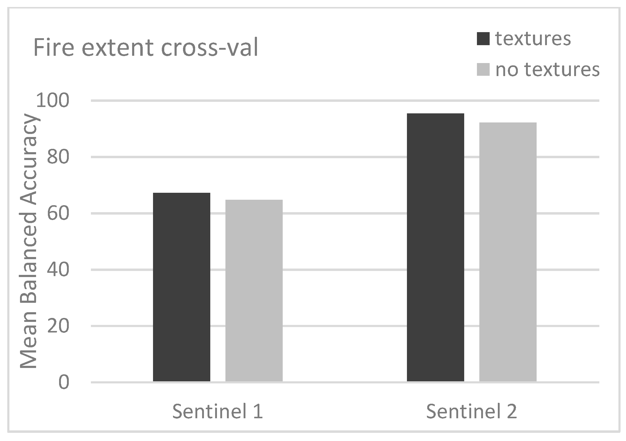
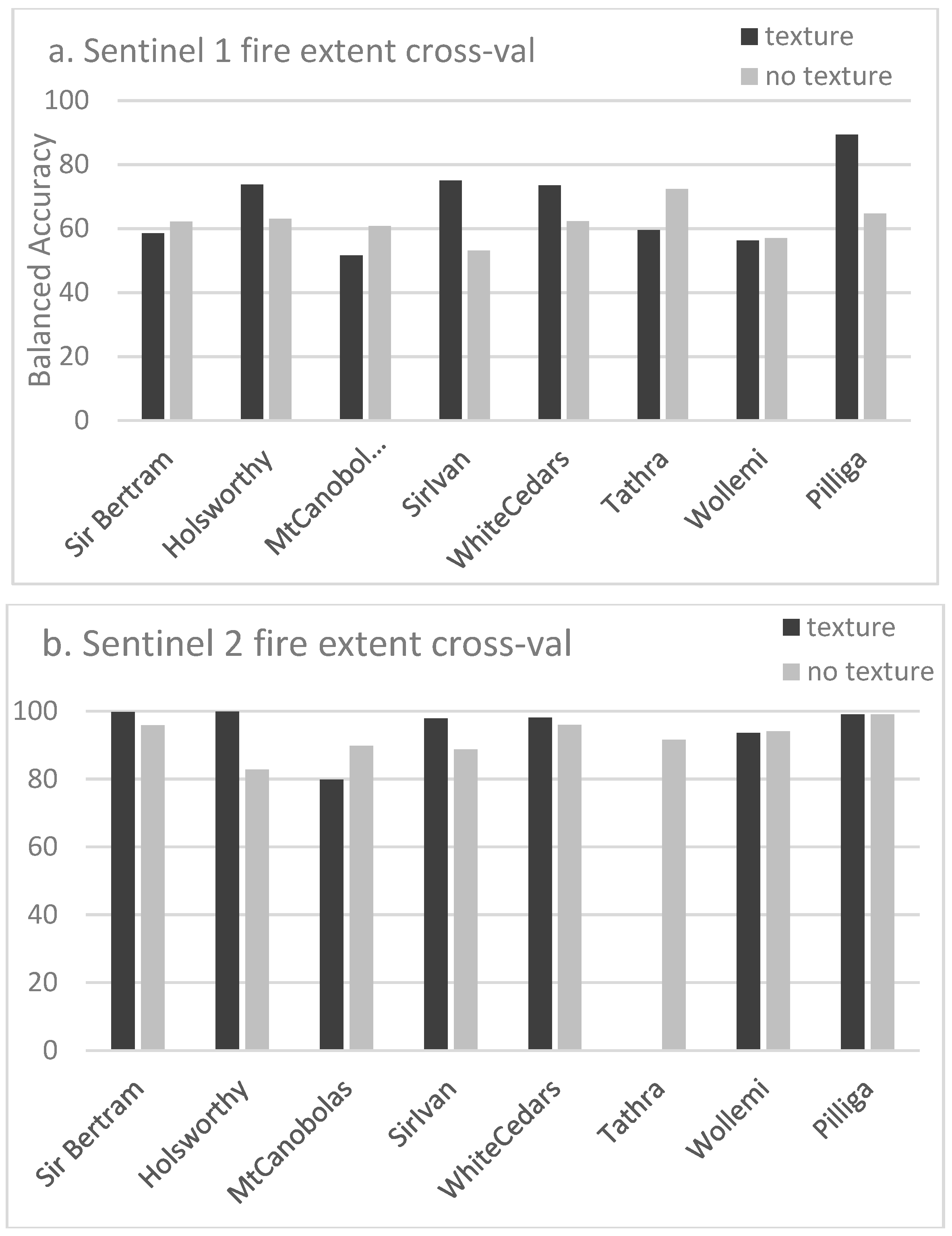
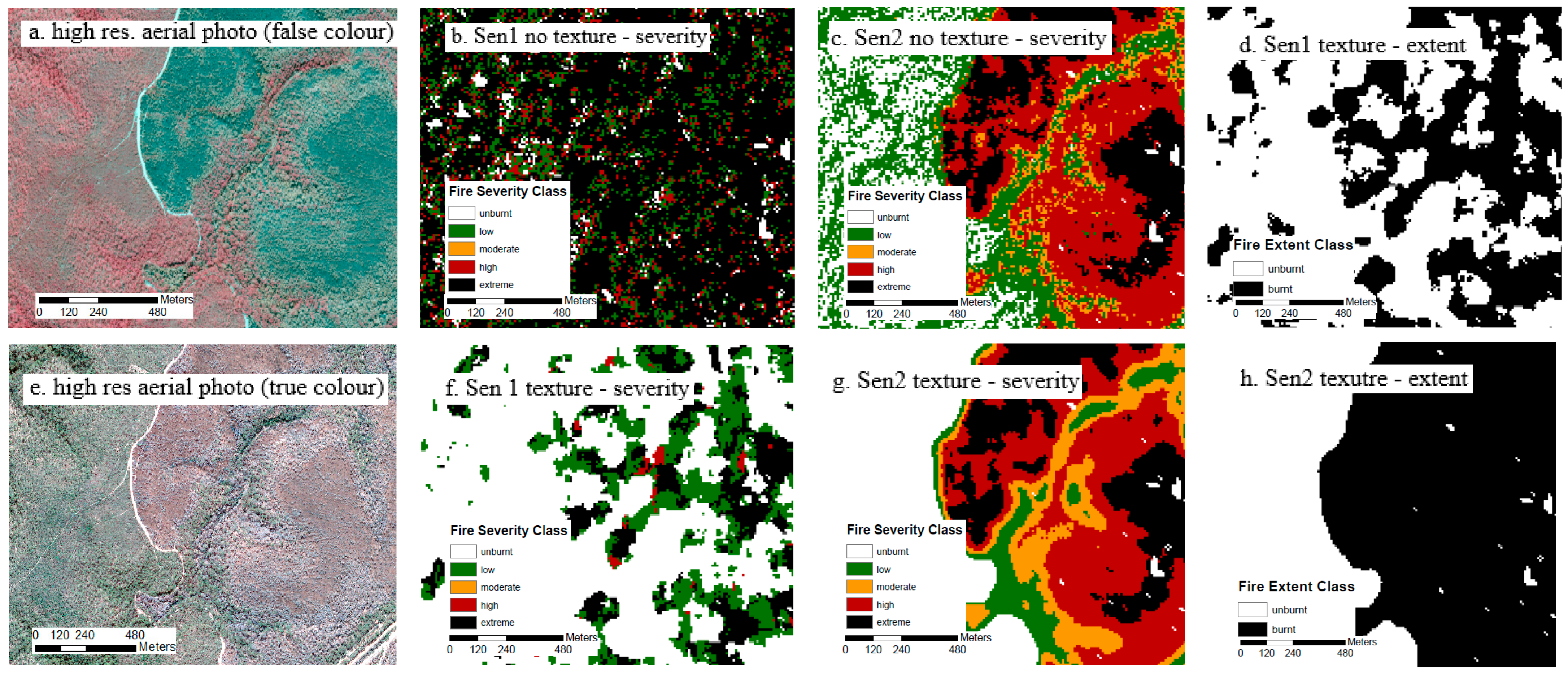
The Sentinel 2 fire extent cross-validation models had 27–28% higher classification accuracy compared to that of Sentinel 1 for both the texture and non-texture models (Figure 4). Texture indices improved the mean balanced accuracy for both the Sentinel 1 and Sentinel 2 fire extent cross-validation models. However, there was high variation between study fires for the Sentinel 1 models. The addition of texture indices improved the classification accuracy at the Holsworthy (11%), Sir Ivan (22%), White Cedars (11%), and Pilliga (25%) case study fires. However, the exclusion of texture indices improved the fire extent classification accuracy at Sir Bertram (4%), Mt Canobolas (9%), Tathra (13%), and Wollemi (1%; Figure 5a). For the Sentinel 2 models, only Mt Canobolas had lower classification accuracy when employing texture models (Figure 5b). High burnt-area-mapping accuracy was demonstrated in the Holsworthy example using Sentinel 2 (Figure 6h), presenting an improved delineation of the burnt perimeter compared to Sentinel 1 (Figure 6d).

3.3. Variable Importance

Variable importance was strongly dominated by optical rather than radar variables in the global combined model of fire severity (Table 4). The mean texture indices for bare cover and dNBR ranked highest among the top 10 variables, followed by non-texture NBR and fractional cover indices. The highest-ranked Sentinel 1 variable (18th) was the VH contrast index.
The highest-ranked variable of importance in the Sentinel 1 fire severity models was the texture index of mean VH across a kernel of 11 (Table 5). The first-order texture metrics and the mean and variance in VH and VV for kernels of both 11 and 7 were all in the top 10 indices (Table 5). Texture metrics estimated using a kernel of 11 ranked higher than those estimated using a kernel of 7 (Table S7, Supplementary Materials), and the texture metrics calculated using VH polarization more frequently occurred in the top 10. The VH and VV backscatter were also included in the top 10 variables in terms of importance, with VH ranked higher. The highest-ranked variable of importance in the Sentinel 2 fire severity models was the non-texture index, RdNBR, followed by the texture indices of mean dNBR and mean dFCBare across kernels of both five and seven (Table 6). Along with the SWIR-based RdNBR2, these indices all ranked higher than the commonly used dNBR.
The variable-of-importance ranks for Sentinel 1 were similar between the fire severity and fire extent models, with the mean and variance texture indices for kernels of both 7 and 11 ranked high in terms of importance. However, the Sentinel 1 VH difference index was ranked among the top 10 with respect to fire extent but not regarding fire severity (Table 7). In contrast, for Sentinel 2, a greater number of texture indices were more highly ranked than RdNBR and dNBR in the fire extent models compared to the fire severity models (Table 8).

4. Discussion

4.1. Sensitivity to Texture Indices

For the Sentinel 2 models, the texture indices increased the classification accuracy across all the severity classes. This constitutes a significant improvement in fire severity mapping following a classical pixel-wise approach [31]. The texture indices added additional information about the neighbourhood context and change in structural characteristics [13] that greatly improved the clustering of pixels belonging to the low- and moderate-severity classes. This result was predicted due to the inherently more heterogenous landscape patterns of these classes compared to the more homogenous higher severities. The greatest proportion of increase in accuracy with the addition of texture indices occurred in the moderate-severity class. Partial canopy scorching presents an inherently high variation in spectral values due to the natural mixture of green (unburnt) and varying degrees of dry (scorched) fractions. The low-severity class, characterised by unburnt canopy surrounded by a matrix of burnt understory, was also endowed with large gains in accuracy with the addition of texture indices for the Sentinel 2 models. Texture indices provide greater sensitivity to small changes in reflectance that may be detected through gaps in the canopy anywhere within the neighbourhood window. By contrast, non-texture indices solely rely on information from a single pixel, which is more likely to be intercepted by the dense canopy. Field validation data would be needed to quantify the limits for mapping low-severity areas under very dense canopy cover, particularly for hazard reduction burns that can typically have areas of unburnt intermixed with patchy very low severity.
The influence of texture indices on the classification accuracy for the Sentinel 1 models was more variable. The addition of texture indices increased the accuracy across all severity classes for the target-trained models only. Increasing fire severity tends to homogenise the landscape, with greater variance in backscatter values in lower-severity classes and unburnt forest regions. The texture information contributed to highlighting the boundary between and magnitude of the backscatter difference between severely burnt and less-impacted forest. Mutai (2019) also demonstrated sensitivity to textural variation using GLCM texture indices derived using the backscattering coefficient to distinguish burnt and unburnt areas [40].
Overall, image texture information enhanced the accuracy of fire extent mapping for both the Sentinel 1 and 2 models, although variation between fires occurred. However, the high variation in the accuracy of the Sentinel 1 texture models between case study fires demonstrates a complex interplay of environmental variables with model performance. Several of the case study fires for which classification accuracy was improved with the implementation of the Sentinel 1 texture models occurred in relatively drier landscapes with more open woodland vegetation structures (e.g., Holsworthy, Sir Ivan, White Cedars, and the Pilliga). There is a tendency toward a larger pre-/post-fire backscatter difference in more open, lower-biomass forest, with greater potential contribution of surface scattering at co-polarizations in severely burnt areas. The inclusion of texture metrics and the mean and variance of the post-fire VH and VH difference improved the discrimination of burnt areas in these open forests. In contrast, the case study fires for which lower classification accuracies were observed with the inclusion of texture indices were generally more topographically complex, occurring in areas with tall, dense, moist forest types (Tathra, Wollemi, and Mt Canobolas). More dense vegetation reduces penetration at the C-band, and saturation is reached more rapidly in high-biomass forests, thereby decreasing the pre-/post-fire backscatter difference and increasing the difficulty of detecting burnt areas. Tanase et al. (2015) also demonstrated greater SAR penetration in drier and sparser canopies than dense, moist canopies [61]. Furthermore, in steeper terrain, it is difficult to detect burnt areas on back-slopes that are within radar shadow. In other studies on SAR texture indices for burnt area mapping, higher entropy was observed over steep burnt areas; however, separability was limited with increasing steepness, with the backscatter affected by incidence angles and shadows. Homogeneity was similarly affected, with limited differences in texture between burnt and unburnt classes in steep areas. Contrast metrics presented the poorest results in steep terrain [40]. Texture metrics cannot significantly improve classification accuracies under these conditions. Indeed, our results show that the case study fires in steeper terrain were superiorly classified without texture indices. Texture indices may increase the neighbourhood window excessively in topographically complex regions, thus rendering pixel-wise approaches superior.
Large window sizes (e.g., 11 × 11 compared to 3 × 3) can decrease random error but may encompass more than one stand type that could introduce systematic error. The data-driven customization of window sizes in lieu of the employment of arbitrary windows has improved estimates of Leaf Area Index (LAI), stand density, and volume [13,54]. The most suitable neighbourhood window size may vary depending on a landscape’s features. Larger window sizes have been used to improve land cover classification accuracies using SAR [62] and more accurately capture homogeneous patterns over large areas [63]. Radar texture indices calculated using a larger window size (11 × 11 compared to 7 × 7) ranked higher in fire severity and burnt extent models. Window size seems more significant in optical burnt area extent models (7 × 7 ranked higher than 5 × 5) compared to fire severity models. Smaller window sizes capture the heterogeneity across small extents [12] but may also increase noise. Texture indices calculated based on more than one window size feature in the top 10 ranked variables in both radar and optical models. This aligns with previous studies showing that land cover classification accuracy is higher when multiple texture features and different window sizes are used [63]. Thus, selecting texture window sizes requires careful consideration and testing with respect to the specific landscape features being targeted.

4.2. Differences Due to Sensor Type

The ability of C-band SAR to detect burnt areas and characterise fire severity is linked to a sensitivity to structural changes. The removal of leaves and twigs in the canopy directly influences the C-band backscattering response, with cross-polarised backscatter decreasing and co-polarised backscatter increasing with fire severity. In the absence of structural change, i.e., in forest areas with only low levels of fire severity, these areas are difficult to distinguish from unburnt forest. This contrasts with the phenomenon observed with optical data, where strong spectral sensitivity is found across the fire severity spectrum [40]. The mechanisms used to detect change are different for SAR and optical data. SAR demonstrates a sensitivity to structural change (physical) within the limits of wavelength, while optical sensors can detect colour changes (bio-chemical) in partially scorched vegetation that remains structurally unchanged. Indeed, in this study, higher mapping accuracies were obtained for all fire severity classes using Sentinel 2.
There are some commonalities between the sensors’ performances across the landscape. The accuracy of fire severity mapping using both optical and SAR data is compromised by topographic complexity and high canopy cover. Radar is also strongly affected by differences in soil and vegetation moisture, which exert a stronger influence in more severely burnt areas with an exposed ground surface. In this study, lower mapping accuracies were observed in topographically complex environments and denser forests using both Sentinel 1 and Sentinel 2; this result aligns with previously reported lower accuracies for low-moderate severity classes in such environments [31].
The target-trained models had greater accuracy than the cross-validation models for both Sentinel 1 and 2, but the increase was much larger for Sentinel 1 with the addition of texture indices. The results indicate the importance of local- vs. regional-scale training data that differ between sensors. The case study sites were highly variable in terms of forest density and structure. This resulted in high variation in the C-band backscattering response, particularly in unburnt and low–moderate severity classes. As radar is more sensitive to forest structural attributes than optical sensors, training data need to capture a wide range of forest types. This would require the use of accurate forest type mapping and may limit the potential of Sentinel 1 in broad-scale applications of fire severity mapping, wherein a robust regional model can be applied to novel fires across the landscape. Even with comprehensive training data, if fire severity differs greatly between sites, so will the ability of C-band SAR to detect burnt areas.
The differences between the sensors may also be explained in part by the technical framework that was used. The simple pre- and post-fire image-differencing method may be better suited to optical sensors with respect to characterising fire effects. Image-differencing techniques for supervised classification have been widely applied in detecting the effects of fires using passive optical data, e.g., Landsat [22,32] and Sentinel 2 [31]. In contrast, studies have demonstrated the adeptness of SAR data with respect to detecting fire effects using deep learning techniques based on multiple data acquisitions across time series to better characterize pre-fire temporal backscatter variations [38] and Sentinel 1 time-series-based burnt area mapping [64]. Speckle noise limits SAR image differencing, particularly in low-severity classes [36].

4.3. Data Fusion

Technological advancements are enabling greater access to high-performance computational capacity, and advances in data fusion approaches are increasingly being realised. Our study demonstrates that the fusion of techniques, namely, per pixel and neighbourhood statistical approaches, into one supervised classification algorithm enhances the accuracy of fire extent and severity mapping using Sentinel 2 and, to a lesser degree, Sentinel 1. Per pixel approaches summarise the pixel values and are less computationally demanding than neighbourhood approaches. However, neighbourhood approaches including texture are useful for characterising vegetation structures [12]. The combination of per pixel and neighbourhood statistical approaches has also been shown to provide additional accuracy in the estimation of forest structure variables such as crown closure, LAI, and stand age [13,54].
Data fusion techniques combining optical and SAR sensors could also offer advantages, as an object or feature that is not seen in a passive sensor image might be seen in an active sensor image and vice versa. There is great potential in leveraging the complementary information provided by the two sensor types [65]). Using multiple sensors can help overcome the limitations of each individual sensor, for example, cloud and smoke limitations in optical images and speckle and variable moisture limitations in SAR [66]. However, comprehensive comparative testing is required to harness the advantages of each sensor type. As our study shows, the random forest supervised classification framework is well suited to Sentinel 2 optical imagery, delivering high accuracy measures with respect to both fire extent and severity. However, when this framework used training data applied to novel fires (cross-validation), severity and burnt area were underestimated using Sentinel 1 due to high variability in the backscattering response with vegetation type and structure, topography, and moisture content.
Deep learning data fusion approaches to image classification using SAR and optical data have recently gained popularity [67,68]. In particular, convolutional neural network (CNN) classifiers demonstrate superior abilities in land cover classification and burnt area mapping compared to traditional machine learning approaches [69]. The use of a CNN has been demonstrated to be advantageous for feature extraction and learning in large-scale analyses involving data fusion [38]. For example, Zhang et al. (2021) demonstrated improved burnt area mapping in California through the synergistic use of Sentinel 2 surface reflectance and Sentinel 1 interferometric coherence in a Siamese Self-Attention (SSA) classifier compared to a random forest (RF) classifier [66]. Lestari et al. (2021) also demonstrated improved burnt-area-mapping performance through the combined classification of SAR and optical data and when using a CNN compared to RF and multilayer perceptron (MLP) classifiers [39]. A hybrid approach developed by Sudiana et al. (2023) involving the employment of a CNN for feature extraction and RF for classification achieved high accuracy (97%) in detecting burnt areas in Central Kalimantan [70]. Precise delineation of burnt areas was achieved through post-processing morphological filtering applied to a U-net classification of Sentinel 1 coherence and Sentinel 2 indices in northern NSW, Australia [69]. Ban et al. (2020) demonstrated effective wildfire progression monitoring using multi-temporal Sentinel 1 data and a CNN framework [38]. The CNN classifier outperformed the traditional log-ratio operator, presenting higher accuracy and better discrimination of the burnt area. Further research into the data fusion of Sentinel 1 and 2 data for mapping severity and the post-fire monitoring of vegetation recovery is recommended.
The integration of data from differing sources enables the generation of complex or derived ecological attributes. For instance, a third dimension can be incorporated into traditional two-dimensional remotely sensed data by using LiDAR [71] and multi-frequency SAR. Airborne and terrestrial laser scanning (TLS) permit the analysis of structural differences beneath the canopy. Depending on the vegetation type, the highest biomass losses can occur in the ground layer, which is not detectable in satellite imagery [36]. Longer-wavelength L-band SAR has been shown to provide better differentiation of fire severity levels, which is largely attributed to the greater penetration depth and sensitivity to woody structures [35]. Post-fire impacts on canopy volume and lower vegetation strata may be discerned using L-band SAR. S-band SAR (9.4 cm wavelength) acquired via NovaSAR and P-band SAR (70 cm) following the launch of BIOMASS may also warrant further investigation for potential application in fire extent and severity mapping. A much longer wavelength, the P-band, may be linked to changes in the understory in fire-affected forests. The coherence of repeat-pass interferometric SAR (InSAR) using pre- and post-fire images may also add useful information about fire severity [72]. Despite the irregular observations, polarimetric decomposition provides information on the scattering mechanisms linked to structural change [73], and further studies are needed to evaluate its use in fire severity estimation.

5. Conclusions

Choosing which set of remotely sensed data to use in ecological studies and land management is a function of what is needed and what is possible. With rapidly changing needs and ever-expanding information resources, advanced image analysis and data fusion techniques are increasing the number of available possibilities for extracting detailed information from a multitude of sources for high-resolution imagery to provided information about forest structures, functions, and ecosystem processes. In this study, we compared the performance of Sentinel 1 (radar) and Sentinel 2 (optical) data with respect to fire severity and extent mapping over a diverse range of forests and topographies in NSW, Australia. The study has contributed new information on the use of SAR-derived GLCM texture metrics for fire severity mapping; such information is not prevalent in the scientific literature. The inclusion of texture indices alongside standard pixel-based metrics was found to increase classification accuracies for both sensor types. The greatest improvements were observed in the higher-severity class when using SAR data and the moderate-severity class when using optical data in the target-trained models. Sentinel 1 texture indices including mean and variance contributed the most to fire severity and extent mapping. The mean dNBR and dFCBare featured prominently in the Sentinel 2 severity models, while a higher number of texture indices contributed to Sentinel 2 extent mapping. Smaller window sizes (5 × 5 or 7 × 7 pixels) were suitable for Sentinel 2, while a larger window size (11 × 11 pixels) was optimal for the computation of texture indices using Sentinel 1 data, although this phenomenon may vary with forest canopy density and topographic complexity.
The influences of dense cover, high biomass, and steep terrain were more evident in the Sentinel 1 models, with the short wavelength of the C-band limiting the detection of burnt areas and severity. Multi-sensor performance was demonstrated using a novel approach to accuracy assessment based on target-trained and cross-validation strategies. Given the high variability in the radar backscattering response to burnt areas, we demonstrated that the use of local training data that capture the difference in relative intensity at a given location and time is important. Our cross-validation results indicate that Sentinel 2 has greater potential to map the fire extent and severity of novel fires compared to Sentinel 1. Future monitoring scenarios will likely continue to focus on the use of optical sensor data for fire extent and severity estimation. Currently, C-band SAR may be useful in instances wherein cloud and smoke limit optical observations, offering the potential to capture most of the severely impacted area. The combined potential of future generations of multi-frequency SAR for severity estimation and for use in analysing specific types of land cover (e.g., heath and grasslands) is the subject of future work. An integrated fire-mapping system that incorporates both active and passive remote sensing for detecting and monitoring changes in vegetation cover and structure would be a valuable resource for future fire management.

Supplementary Materials

The following supporting information can be downloaded at: https://www.mdpi.com/article/10.3390/rs15143512/s1, Figure S1: Method workflow; Figure S2: Example severity class training and validation data derived from high resolution aerial photography; Table S1: Sentinel 1 fire severity cross validation models a. with texture indices, b. without texture indices; Table S2: Sentinel 1 fire-severity target-trained models, a. with texture indices, b. without texture indices; Table S3: Sentinel 2 fire severity cross validation models, a. with texture indices, b. without texture indices; Table S4: Sentinel 2 fire severity target-trained models, a. with texture indices, b. without texture indices; Table S5: Sentinel 1 fire extent cross-validation models a. with texture indices, b. without texture indices; Table S6: Sentinel 2 fire extent cross-validation models a. with texture indices, b. without texture indices; Table S7: Ranked Gini Index values for Sentinel 1 cross validation models; Table S8: Ranked Gini Index values for Sentinel 2 cross-validation models;.

Author Contributions

R.K.G. conceptualised and directed the study, prepared data, undertook analyses, produced the tables and figures, and was the lead writer. A.M. and H.-C.C. prepared the data and contributed to the writing and editing of the manuscript. All authors have read and agreed to the published version of the manuscript.

Funding

Funded in part by the Natural Resources Commission Forest Monitoring and Improvement Program’s Foundational Priority Projects scheme. Further support for the research was provided by the NSW DPIE science department and UNSW. We thank the several peer-reviewers for their helpful comments applied to draft versions of the manuscript.

Data Availability Statement

Sentinel 1 and 2 tiles are available for download from the Copernicus Australasia Regional Data Hub (https://www.copernicus.gov.au/, accessed on 1 July 2022), and fractional cover products are publicly available through the TERN AusCover server (www.auscover.org.au accessed 1 July 2022).

Acknowledgments

We acknowledge the traditional custodians and knowledge holders of the country where we conducted our research, walk, and live. We pay our respects to Elders past, present, and emerging.

Conflicts of Interest

The authors declare no conflict of interest.

References

  1. Belward, A.S.; Skoien, J.O. Who launched what, when and why: Trends in global land-cover observation capacity from civilian earth observation satellites. ISPRS J. Photogramm. Remote Sens. 2015, 103, 115–128. [Google Scholar] [CrossRef]
  2. Wekerle, T.; Filho, J.B.P.; da Costa, L.E.V.L.; Trabasso, L.G. Status and trends of Smallsats and their launch vehicles - an up-to-date review. J. Aerosp. Technol. Manag. 2017, 9, 269. [Google Scholar] [CrossRef]
  3. Peral, E.; Im, E.; Wye, L.; Lee, S.; Tanelli, S.; Rahmat-Samii, Y.; Horst, S.H. Radar technologies for earth remote sensing from CubeSat platforms. Proc. IEEE 2018, 106, 404–418. [Google Scholar] [CrossRef]
  4. Liao, X.; Zhang, Y.; Su, F.; Yue, H.; Ding, Z.; Liu, J. UAVs surpassing satellites and aircraft in remote sensing over China. Int. J. Remote Sens. 2018, 39, 7138–7153. [Google Scholar] [CrossRef]
  5. Manfreda, S.; McCabe, M.F.; Miller, P.; Lucas, R.; Madrigal, V.P.; Mallinis, G.; Dor, E.B.; Helman, D.; Estes, L.; Ciraolo, G.; et al. On the use of unmanned aerial systems for environmental monitoring. Remote Sens. 2018, 10, 641. [Google Scholar] [CrossRef] [Green Version]
  6. Chen, Z.; Pasher, J.; Duffe, J.; Behnamian, A. Mapping arctic coastal ecosystems with high resolution optical satellite imagery using a hybrid classification approach. Can. J. Remote Sens. 2017, 43, 513–527. [Google Scholar] [CrossRef]
  7. Dhingra, S.; Kumar, D. A review of remotely sensed satellite image classifiacation. Int. J. Electr. Comput. Eng. 2019, 9, 1720–1731. [Google Scholar]
  8. Sghaier, M.O.; Hammami, I.; Foucher, S.; Lepage, R. Flood extent mapping from time-series SAR images based on texture analysis and data fusion. Remote Sens. 2018, 10, 237. [Google Scholar] [CrossRef] [Green Version]
  9. Mohanaiah, P.; Sathyanarayana, P.; GuruKumar, L. Image texture feature extraction using GLCM approach. Int. J. Sci. Res. Publ. 2013, 3, 2250–3153. [Google Scholar]
  10. Guo, W.; Rees, W.G. Altitudinal forest-tundra ecotone categorisation using texture-based classification. Remote Sens. Environ. 2019, 232, 111312. [Google Scholar] [CrossRef]
  11. Murray, H.; Lucieer, A.; Williams, R. Texture-based classification of sub-Antarctic vegetation communities on Heard island. Int. J. Appl. Earth Obs. Geoinf. 2010, 12, 138–149. [Google Scholar] [CrossRef]
  12. Wood, E.M.; Pidgeon, A.M.; Radeloff, V.C.; Keuler, N.S. Image texture as a remotely sensed measure of vegetation structure. Remote Sens. Environ. 2012, 121, 516–526. [Google Scholar] [CrossRef]
  13. Wulder, M. Optical remote-sensing techniques for the assessment of forest inventory and biophysical parameters. Prog. Phys. Geogr. 1998, 22, 449–476. [Google Scholar] [CrossRef]
  14. Liu, D.; Kelly, M.; Gong, P. A spatial-temporal approach to monitoring forest disease spread using multi-temporal high spatial resolution imagery. Remote Sens. Environ. 2006, 101, 167–180. [Google Scholar] [CrossRef]
  15. Haralick, R.M.; Shanmugam, K.; Dinstein, I. Textural features for image classification. IEEE Trans. Syst. Man Cybern. 1973, 3, 610–621. [Google Scholar] [CrossRef] [Green Version]
  16. Hall-Beyer, M. Practical guidelines for choosing GLCM textures to use in landscape classification tasks over a range of moderate spatial scales. Int. J. Remote Sens. 2017, 38, 1312–1338. [Google Scholar] [CrossRef]
  17. Keeley, J.E. Fire intensity, fire severity and burn severity—A brief review and suggested usage. Int. J. Wildland Fire 2009, 18, 116–126. [Google Scholar] [CrossRef]
  18. Chafer, C.J.; Noonan, M.; Macnaught, E. The post-fire measurement of fire severity and intensity in the Christmas 2001 Sydney wildfires. Int. J. Wildland Fire 2004, 13. [Google Scholar] [CrossRef]
  19. Lentile, L.B.; Holden, Z.A.; Smith, A.M.S.; Falkowski, M.J.; Hudak, A.T. Remote sensing techniques to assess active fire characteristics and post-fire effects. Int. J. Wildland Fire 2006, 15, 319–345. [Google Scholar] [CrossRef]
  20. Miller, J.D.; Thode, A.E. Quantifying burn severity in a heterogenous landscape with a relative version of the delta Normalized Burn Ratio (dNBR). Remote Sens. Environ. 2007, 109, 66–80. [Google Scholar] [CrossRef]
  21. Hall, R.J.; Freeburn, J.T.; de Groot, W.J.; Pritchard, J.M.; Lynham, T.J.; Landry, R. Remote sensing of burn severity: Experience from western Canada boreal fires. Int. J. Wildland Fire 2008, 17, 476–489. [Google Scholar] [CrossRef]
  22. Cansler, C.A.; McKenzie, D. Climate, fire size and biophysical setting control fire severity and spatial pattern in the northern Cascade Range, USA. Ecol. Appl. 2014, 24, 1037–1056. [Google Scholar] [CrossRef]
  23. Pettorelli, N.; Laurance, W.F.; O’Brien, T.G.; Wegmann, M.; Nagendra, H.; Turner, W. Satellite remote sensing for applied ecologists: Opportunities and challenges. J. Appl. Ecol. 2014, 51, 839–848. [Google Scholar] [CrossRef]
  24. Miller, J.D.; Knapp, E.E.; Key, C.H.; Skinner, C.N.; Isbell, C.J.; Creasy, R.M.; Sherlock, J.W. Calibration and validation of the relative differenced Normalised Burn Ration (RdNBR) to three measures of fire severity in the Sierra Nevada and Klamath Mountains, California, USA. Remote Sens. Environ. 2009, 113, 645–656. [Google Scholar] [CrossRef]
  25. Hoy, E.E.; French, N.H.F.; Turetsky, M.R.; Trigg, S.N.; Kasischke, E.S. Evaluating the potential of Landsat TM/ETM+ imagery for assessing fire severity in Alaskan black spruce forests. Int. J. Wildland Fire 2008, 17, 500–514. [Google Scholar] [CrossRef]
  26. Smith, A.M.S.; Eitel, J.U.H.; Hudak, A.T. Spectral analysis of charcoal on soils: Implications for wildland fire severity mapping methods. Int. J. Wildland Fire 2010, 19, 976–983. [Google Scholar] [CrossRef]
  27. Marino, E.; Guillen-Climent, M.; Ranz, P.; Tome, J.L. Fire severity mapping in Garajonay National Park: Comparison between spectral indices. FLAMMA 2014, 7, 22–28. [Google Scholar]
  28. Epting, J.; Verbyla, D.; Sorbel, B. Evaluation of remotely sensed indices for assessing burn severity in interior Alaska using Landsat TM and ETM+. Remote Sens. Environ. 2005, 96, 328–339. [Google Scholar] [CrossRef]
  29. Morgan, P.; Keane, R.E.; Dillon, G.K.; Jain, T.B.; Hudak, A.T.; Karau, E.C.; Sikkink, P.G.; Holden, Z.A.; Strand, E.K. Challenges of assessing fire and burn severity using field measures, remote sensing and modelling. Int. J. Wildland Fire 2014, 23, 1045–1060. [Google Scholar] [CrossRef] [Green Version]
  30. Meddens, A.J.H.; Kolden, C.A.; Lutz, J.A. Detecting unburned areas within wildfire perimeters using Landsat and ancillary data across the northwestern United States. Remote Sens. Environ. 2016, 186, 275–285. [Google Scholar] [CrossRef]
  31. Gibson, R.; Danaher, T.; Hehir, W.; Collins, L. A remote sensing approach to mapping fire severity in south-eastern Australia using sentinel 2 and random forest. Remote Sens. Environ. 2020, 240, 111702. [Google Scholar] [CrossRef]
  32. Collins, L.; Griffioen, P.; Newell, G.; Mellor, A. The utility of Random Forests in Google Earth Engine to improve wildfire severity mapping. Remote Sens. Environ. 2018, 216, 374–384. [Google Scholar] [CrossRef]
  33. Sinha, S.; Jeganathan, C.; Sharma, L.K.; Nathawat, M.S. A review of radar remote sensing for biomass estimation. Int. J. Environ. Sci. Technol. 2015, 12, 1779–1792. [Google Scholar] [CrossRef] [Green Version]
  34. Treuhaft, R.N.; Law, B.E.; Asner, G.P. Forest attributes from radar interferometric structure and its fusion with optical remote sensing. Bioscience 2004, 54, 561–571. [Google Scholar] [CrossRef] [Green Version]
  35. Tanase, M.A.; Santoro, M.; De La Riva, J.; Pérez-Cabello, F.; Le Toan, T. Sensitivity of X-, C- and L-band SAR backscatter to burn severity in Mediterranean Pine forests. IEEE Trans. Geosci. Remote Sens. 2010, 48, 3663–3675. [Google Scholar] [CrossRef]
  36. Philipp, M.B.; Levick, S.R. Exploring the potential of C-band SAR in contributing to burn severity mapping in tropical savanna. Remote Sens. 2020, 12, 49. [Google Scholar] [CrossRef] [Green Version]
  37. Plank, S.; Karg, S.; Martinis, S. Full polarimetric burn scar mapping-the differences of active fire and post-fire situations. Int. J. Remote Sens. 2019, 40, 253–268. [Google Scholar] [CrossRef]
  38. Ban, Y.; Zhang, P.; Nascetti, A.; Bevington, A.R.; Wilder, M.A. Near real-time wildfire progression monitoring with Sentinel-1 SAR time series and deep-learning. Nat. Sci. Rep. 2000, 10, 1322. [Google Scholar] [CrossRef] [Green Version]
  39. Lestari, A.I.; Rizkinia, M.; Sudiana, D. Evaluation of combining optical and SAR imagery for burned area mapping using machine learning. In Proceedings of the IEEE 11th Annual Computing and Communication Workshop and Conference, Las Vegas, NV, USA, 27–30 January 2021. [Google Scholar]
  40. Mutai, S.C. Analysis of Burnt Scar Using Optical and Radar Satellite Data; University of Twente: Enschede, The Netherlands, 2019. [Google Scholar]
  41. Tariq, A.; Jiango, Y.; Lu, L.; Jamil, A.; Al-ashkar, I.; Kamran, M.; El Sabagh, A. Integrated use of Sentinel-1 and Sentinel-2 and open-source machine learning algorithms for burnt and unburnt scars. Geomat. Nat. Hazards Risk 2023, 14. [Google Scholar] [CrossRef]
  42. Hutchinson, M.F.; McIntyre, S.; Hobbs, R.J.; Stein, J.L.; Garnett, S.; Kinloch, J. Integrating a global agro-climatic classification with bioregional boundaries in Australia. Glob. Ecol. Biogeogr. 2005, 14, 197–212. [Google Scholar] [CrossRef]
  43. Filipponi, F. Sentinel-1 GRD preprocessing workflow. In Proceedings of the 3rd International Electronic Conference on Remote Sensing, Online, 22 May–5 June 2019. [Google Scholar]
  44. Chini, M.; Pelich, R.; Hostache, R.; Matgen, P.; Lopez-Martinez, C. Towards a 20m global building map from Sentinel-1 SAR data. Remote Sens. 2018, 10, 1833. [Google Scholar] [CrossRef] [Green Version]
  45. Sen, P.K. Estimates of the regression coefficient based on Kendall’s tau. J. Am. Statisics Assoc. 1968, 63, 1379–1389. [Google Scholar] [CrossRef]
  46. Flood, N.; Danaher, T.; Gill, T.; Gillingham, S. An operational scheme for deriving standardised surface reflectance from Landsat TM/ETM+ and SPOT HRG imagery for eastern Australia. Remote Sens. 2013, 5, 83–109. [Google Scholar] [CrossRef] [Green Version]
  47. Farr, T.G.; Rosen, P.A.; Caro, E.; Crippen, R.; Duren, R.; Hensley, S.; Kobrick, M.; Paller, M.; Rodriguez, E.; Roth, L.; et al. The Shuttle Radar Topography Mission. Rev. Geophys. 2007, 45. [Google Scholar] [CrossRef] [Green Version]
  48. Gallant, J.; Read, A. Enhancing the SRTM Data for Australia. Proc. Geomorphometry 2009, 31, 149–154. [Google Scholar]
  49. Guerschman, J.P.; Scarth, P.F.; McVicar, T.R.; Renzullo, L.J.; Malthus, T.J.; Stewart, J.B.; Rickards, J.E.; Trevithick, R. Assessing the effects of site heterogeneity and soil properties when unmixing photosynthetic vegetation, non-photosynthetic vegetation and bare soil fractions for Landsat and MODIS data. Remote Sens. Environ. 2015, 161, 12–26. [Google Scholar] [CrossRef]
  50. Morresi, D.; Vitali, A.; Urbinati, C.; Garbarino, M. Forest Spectral Recovery and Regeneration Dynamics in Stand-Replacing Wildfires of Central Apennines Derived from Landsat Time Series. Remote Sens. 2020, 11, 308. [Google Scholar] [CrossRef] [Green Version]
  51. Yu, H.; Zhang, Z. New Directions: Emerging satellite observations of above-cloud aerosols and direct radiative forcing. Atmos. Environ. 2013, 72, 36–40. [Google Scholar] [CrossRef] [Green Version]
  52. Zvoleff, A.; Calculate textures from Grey-level Co-occurrence Matrices (GLCMs). R Statisical Computing Software: 2022. Available online: https://www.r-project.org/ (accessed on 1 July 2022).
  53. Dorigo, W.; Lucieer, A.; Podobnikara, T.; Carnid, A. Mapping invasive Fallopia japonica by combined spectral, spatial and temporal analysis of digital orthophotos. Int. J. Appl. Earth Obs. Geoinf. 2012, 19, 185–195. [Google Scholar] [CrossRef]
  54. Franklin, S.E.; Hall, R.J.; Moskal, L.M.; Lavigne, M.B. Incorporating texture into classification of forest species composition from airborne multispectral images. Int. J. Remote Sens. 2000, 21, 61–79. [Google Scholar] [CrossRef]
  55. Kuhn, M.; Wing, J.; Weston, S.; Williams, A.; Keefer, C.; Engelhardt, A.; Cooper, T.; Mayer, Z.; Kenkel, B. Classification and Regression Training; R Statistical Computing Software. 2023. Available online: https://www.r-project.org/ (accessed on 1 July 2022).
  56. Breiman, L.; Friedman, J.H.; Olshen, R.A.; Stone, C.J. Classification and Regression Trees; Wadsworth International Group: Belmont, CA, USA, 1984. [Google Scholar]
  57. Breiman, L. Random Forests. Mach. Learn. 2001, 5, 5–32. [Google Scholar] [CrossRef] [Green Version]
  58. Millard, K.; Richardson, M. On the importance of training data sample selection in random forest image classification: A case study in peatland ecosystem mapping. Remote Sens. 2015, 7, 8489–8515. [Google Scholar] [CrossRef] [Green Version]
  59. Hudak, A.T.; Robichaud, P.R.; Evans, J.S.; Clark, J.; Lannom, K.; Morgan, P.; Stone, C. Field validation of burned area reflectance classification (BARC) products for post fire assessment. In Remote Sensing for Field Users, Proceedings of the Tenth Forest Service Remote Sensing Applications Conference, Salt Lake City, Utah, 5–9 April 2004; American Society of Photogrammetry and Remote Sensing: Salt Lake City, UT, USA, 2004; p. 13. [Google Scholar]
  60. McCarthy, G.; Moon, K.; Smith, L. Mapping fire severity and fire extent in forest in Victoria for ecological and fuel outcomes. Ecol. Manag. Restor. 2017, 18, 54–64. [Google Scholar] [CrossRef]
  61. Tanase, M.A.; Kennedy, R.; Aponte, C. Radar burn ratio for fire severity estimation at canopy level: An example for temperate forests. Remote Sens. Environ. 2015, 170, 14–31. [Google Scholar] [CrossRef]
  62. Otukei, J.R.; Blaschke, T.; Collins, M. A decision tree approach for identifying the optimum window size for extracting texture features from TerraSAR-X data. Environ. Sci. Math. 2012. [Google Scholar]
  63. Zhou, T.; Li, Z.; Pan, J. Multi-feature classification of multi-sensors satellite imagery based on dual-polarimetric Sentinel-1A, Landsat-8 OLI and Hyperion images for urban land-cover classification. Sensors 2018, 18, 373. [Google Scholar] [CrossRef] [Green Version]
  64. Belenguer-Plomer, M.A.; Tanase, M.; Fernandez-Carrillo, A.; Chuvieco, E. Burned area detection and mapping using Sentinel-1 backscatter coefficient and thermal anomalies. Remote Sens. Environ. 2019, 233, 111345. [Google Scholar] [CrossRef]
  65. Amarsaikhan, D.; Douglas, T. Data fusion and multisource image classification. Int. J. Remote Sens. 2010, 25, 3529–3539. [Google Scholar] [CrossRef]
  66. Zhang, Q.; Ge, L.; Zhang, R.; Metternicht, G.I.; Du, Z.; Kuang, J.; Xu, M. Deep-learning-based burned area mapping using the synergy of Sentinel-1 and 2 data. Remote Sens. Environ. 2021, 264, 112575. [Google Scholar] [CrossRef]
  67. Alencar, A.A.; Arruda, V.L.S.; da Silva, W.V.; Conciani, D.E.; Costa, D.P.; Crusco, N.; Duverger, S.G.; Ferreira, N.C.; Franca-Rocha, W.; Hasenack, H.; et al. Long-Term Landsat-Based Monthly Burned Area Dataset for the Brazilian Biomes Using Deep Learning. Remote Sens. 2022, 14, 2510. [Google Scholar] [CrossRef]
  68. Farasin, A.; Colomba, L.; Garza, P. Double-Step U-Net: A Deep Learning-Based Approach for the Estimation of Wildfire Damage Severity through Sentinel-2 Satellite Data. Appl. Sci. 2020, 10, 4332. [Google Scholar] [CrossRef]
  69. Lee, I.K.; Trinder, J.C.; Sowmya, A. Application of U-net convolutional neural network to bushfire monitoring in Australia with Sentinel-1/2 data. Int. Arch. Photogramm. Remote Sens. Spat. Inf. Sci. 2020, XLIII-B1-2020, 573–578. [Google Scholar] [CrossRef]
  70. Sudiana, D.; Lestari, A.I.; Riyanto, I.; Rizkinia, M.; Arief, R.; Prabuwono, A.S.; Sumantyo, J.T.S. A hybrid convolutional neural network and random forest for burned area identification with optical and synthetic aperture radar (SAR) data. Remote Sens. 2023, 15, 728. [Google Scholar] [CrossRef]
  71. Lefsky, M.A.; Cohen, W.B.; Parker, G.G.; Harding, D.J. Lidar remote sensing for ecosystem studies. Bioscience 2002, 52, 19–30. [Google Scholar] [CrossRef]
  72. Tanase, M.A.; Santoro, M.; Wegmüller, U.; De La Riva, J.; Pérez-Cabello, F. Properties of X-, C- and L-band repeat-pass interferometric SAR coherence in Mediterranean pine forests affected by fires. Remote Sens. Environ. 2010, 114, 2182–2194. [Google Scholar] [CrossRef]
  73. Tanase, M.A.; Santoro, M.; Aponte, C.; De La Riva, J. Polarimetric properties of burned forest areas at C- and L-band. IEEE J. Sel. Top. Appl. Earth Obs. Remote Sens. 2014, 7, 267–276. [Google Scholar] [CrossRef]
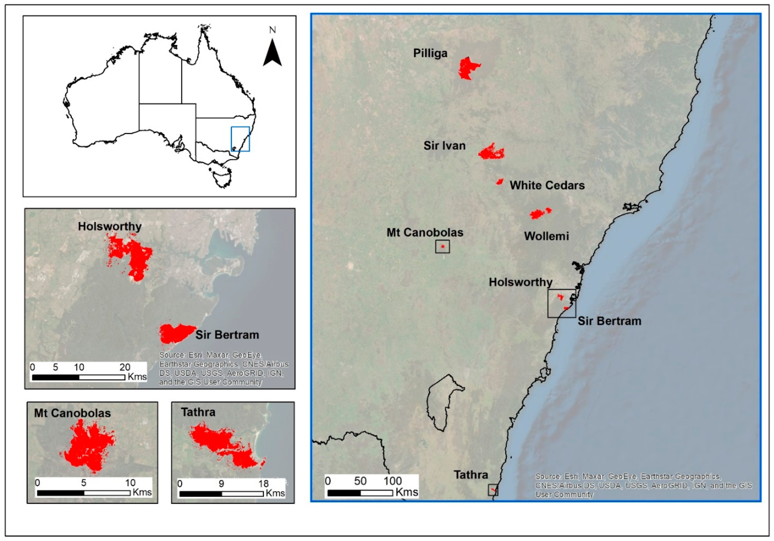
Figure 1. Location of the 8 case study fires (Pilliga, Sir Ivan, White Cedars, Mt Canobolas, Wollemi, Holsworthy, Sir Bertram, and Tathra) in NSW, Australia.
Remotesensing 15 03512 g001
Figure 2. Mean balanced accuracy metrics across texture indices and fire severity classes for Sentinel 1 (a) cross-validation models and (b) target-trained models.
Remotesensing 15 03512 g002
Figure 3. Mean balanced accuracy metrics across texture indices and fire severity classes for Sentinel 2 (a) cross-validation models and (b) target-trained models.
Remotesensing 15 03512 g003
Figure 4. Mean balanced accuracy of the unburnt class for fire extent models across texture types (texture/no texture indices) and sensor types (Sentinel 1/Sentinel 2).
Remotesensing 15 03512 g004
Figure 5. The variation between study fires in terms of balanced accuracy for fire extent cross-validation models with and without texture indices for (a) Sentinel 1 and (b) Sentinel 2.
Remotesensing 15 03512 g005
Figure 6. Visual examples of results for a sample of cross-validation models of the Holsworthy fire; (a) high-resolution post-fire aerial photography in near-infrared false colour display, (b) Sentinel 1 fire severity model excluding texture indices, (c) Sentinel 2 fire severity model excluding texture indices, (d) Sentinel 1 fire extent model including texture indices, (e) high-resolution post-fire aerial photography in true colour display, (f) Sentinel 1 fire severity model including texture indices, (g) Sentinel 2 fire severity model including texture indices, and (h) Sentinel 2 fire extent model including texture indices.
Remotesensing 15 03512 g006
Table 1. Summary of case study fires with start and end dates and details on high-resolution photography (airborne digital sensor, ADS) used for aerial photo interpretation (API). The number of days for which the photos were captured after the end of a fire is included in parentheses.
Fire NameFire Start DateFire End Date Aerial PhotographyDate of CaptureFire Size (Ha)
Sir Ivan11 February 201717 February 201750 cm 4-band ADS18 February 2017 (1)47,105
White Cedars12 February 201717 February 201720 cm 4-band ADS16 February 2017 (−1)5217
Wollemi18 January 201815 February 201850 cm 4-band ADS17 March 2018 (30)14,178
Mt Canobolas10 February 201815 February 201830 cm 4-band ADS9 March 2018 (21)1891
Sir Bertram20 January 2018 15 January 201850 cm 4-band ADS11 March 2018 (38)2241
Pilliga19 January 201825 February 201850 cm 4-band ADS11 March 2018 (38)57,822
Tathra18 March 201819 March 201810 cm 4-band ADS20 March 2018 (1)1258
Holsworthy13 April 201818 April 201850 cm 4-band ADS24 April 2018 (6)3955
Table 2. Index definitions. Variable names are composed of the base index, an abbreviation of the GLCM metric, and the kernel size. Abbreviations include ‘var’ (variance), ‘2mom’ (2nd moment), con (contrast), ‘corr’ (correlation), ‘dissim’ (dissimilarity), and ‘hom’ (homogeneity).
SensorBase IndexTexture MetricTexture TypeKernelsVariable Names
Sentinel 1dVHNoneNoneNoneradar_inputVH
Sentinel 1dVHMean 1st order7, 11glcm_radarVH_mean_7glcm_radarVH_mean_11
Sentinel 1dVHVariance1st order7, 11glcm_radarVH_var_7glcm_radarVH_var_11
Sentinel 1dVH2nd moment2nd order7, 11glcm_radarVH_2mom_7glcm_radarVH_2mom_11
Sentinel 1dVHContrast2nd order7, 11glcm_radarVH_con_7glcm_radarVH_con_11
Sentinel 1dVHCorrelation2nd order7, 11glcm_radarVH_corr_7glcm_radarVH_corr_11
Sentinel 1dVHDissimilarity2nd order7, 11glcm_radarVH_dissim_7glcm_radarVH_dissim_11
Sentinel 1dVHHomogeneity2nd order7, 11glcm_radarVH_hom_7glcm_radarVH_hom_11
Sentinel 1dVVNoneNone7, 11radar_inputVV
Sentinel 1dVVMean 1st order7, 11glcm_radarVV_mean_7glcm_radarVV_mean_11
Sentinel 1dVVVariance1st order7, 11glcm_radarVV_var_7glcm_radarVV_var_11
Sentinel 1dVV2nd moment2nd order7, 11glcm_radarVV_2mom_7glcm_radarVV_2mom_11
Sentinel 1dVVContrast2nd order7, 11glcm_radarVV_con_7glcm_radarVV_con_11
Sentinel 1dVVCorrelation2nd order7, 11glcm_radarVV_corr_7glcm_radarVV_corr_11
Sentinel 1dVVDissimilarity2nd order7, 11glcm_radarVV_dissim_7glcm_radarVV_dissim_11
Sentinel 1dVVHomogeneity2nd order7, 11glcm_radarVV_hom_7glcm_radarVV_hom_11
Sentinel 2NBRNoneNoneNonedNBRRdNBR
Sentinel 2NBR2NoneNoneNoneSWIR_dNBR2SWIR_RdNBR2
Sentinel 2Fractional Cover NoneNoneNoneRdFCTotaldFCBare
Sentinel 2dFCBareMean 1st order5, 7mean_dFCBare_5mean_dFCBare_7
Sentinel 2dFCBareVariance1st order5, 7var_dFCBare_5var_dFCBare_7
Sentinel 2dNBRMean 1st order5, 7mean_dNBR_5mean_dNBR_7
Sentinel 2dNBRVariance1st order5, 7var_dNBR_5var_dNBR_7
Sentinel 2SWIR_dNBR2Mean 1st order5, 7glcm_SWIR_dNBR2_mean_5glcm_SWIR_dNBR2_mean_7
Sentinel 2SWIR_dNBR2Variance1st order5, 7glcm_SWIR_dNBR2_var_5glcm_SWIR_dNBR2_var_7
Sentinel 2SWIR_dNBR22nd moment2nd order5, 7glcm_SWIR_dNBR2_2mom_5glcm_SWIR_dNBR2_2mom_7
Sentinel 2SWIR_dNBR2Contrast2nd order5, 7glcm_SWIR_dNBR2_con_5glcm_SWIR_dNBR2_con_7
Sentinel 2SWIR_dNBR2Correlation2nd order5, 7glcm_SWIR_dNBR2_corr_5glcm_SWIR_dNBR2_corr_7
Sentinel 2SWIR_dNBR2Dissimilarity2nd order5, 7glcm_SWIR_dNBR2_dissim_5glcm_SWIR_dNBR2_dissim_7
Sentinel 2SWIR_dNBR2Homogeneity2nd order5, 7glcm_SWIR_dNBR2_hom_5glcm_SWIR_dNBR2_hom_7
NARandom pixelsNoneNoneNonerandom
Table 3. Fire severity class labels and definitions adapted from Hudak et al. (2004) [59], McCarthy et al. (2017) [60], Collins et al. (2018) [32], and Gibson et al. (2020) [31].
Pixel ColourSeverity ClassDefinition% Foliage Affected by FireN Sampling Points
Remotesensing 15 03512 i001UnburntUnburnt 0% of canopy and understory burnt40,257
Remotesensing 15 03512 i002LowBurnt surface with unburnt canopy>10% of understory burnt
>90% green canopy
11,198
Remotesensing 15 03512 i003ModeratePartial canopy scorched 20–90% of canopy scorched7142
Remotesensing 15 03512 i004HighFull canopy scorched (+/− partial canopy consumption)>90% of canopy scorched
<50% of canopy biomass consumed
24,479
Remotesensing 15 03512 i005ExtremeFull canopy consumption >50% of canopy biomass consumed20,760
Table 4. Mean decrease in the Gini Index and corresponding relative rank positions for the combined Sentinel 1 and Sentinel 2 global fire severity model. * denotes the highest-ranked Sentinel 1 index.
IndicesMean Decrease GiniRelative Rank
mean_dFCBare712621
mean_dFCBare511122
mean_dNBR78323
mean_dNBR58034
RdNBR7625
dFCBare7316
RdFCTotal5577
dNBR5428
SWIR_RdNBR23849
SWIR_dNBR232710
glcm_SWIR_dNBR2_mean_727311
glcm_SWIR_dNBR2_var_726812
var_dFCBare724913
glcm_SWIR_dNBR2_mean_524114
glcm_SWIR_dNBR2_var_522615
var_dFCBare516816
var_dNBR710617
glcm_radarVH_con_1110118 *
glcm_radarVH_mean_119919
var_dNBR59720
rndm3161
Table 5. Top-10-ranking Gini index values for Sentinel 1 cross-validation fire severity models.
Sentinel 1 Fire Severity IndicesAverage Rank
glcm_radarVH_mean_111.5
glcm_radarVH_var_111.8
glcm_radarVV_var_114.1
glcm_radarVV_mean_114.3
glcm_radarVH_var_75.6
glcm_radarVH_mean_75.9
VHbackscatter7.0
glcm_radarVH_con_119.1
VVbackscatter9.4
glcm_radarVV_var_710.1
Table 6. Top 10 Gini index values for Sentinel 2 cross-validation fire severity models.
Sentinel 2 Fire Severity IndicesAverage Rank
RdNBR1.3
mean_dNBR53.1
mean_dNBR73.1
mean_dBare73.6
mean_dBare54.1
SWIR_RdNBR26.5
dNBR7.5
dBare8.3
glcm_SWIR_dNBR2_var_79.6
SWIR_dNBR210.1
Table 7. Top 10 Gini index values for Sentinel 1 cross-validation fire extent models.
Sentinel 1 Fire Extent IndicesAverage Rank
glcm_radarVH_var_113
glcm_radarVV_mean_115.9
glcm_radarVH_mean_116
glcm_radarVV_var_116.2
glcm_radarVH_var_77.4
glcm_radarVH_mean_79.2
radar_inputVH9.2
glcm_radarVV_mean_710.7
glcm_radarVV_var_711.5
glcm_radarVH_2mom_1111.7
VHbackscatter12.2
Table 8. Top 10 Gini index values for Sentinel 2 cross-validation fire extent models.
Sentinel 2 Fire Extent IndicesAverage Rank
mean_dBare76.0
mean_dNBR76.0
glcm_SWIR_dNBR2_mean_76.4
glcm_SWIR_dNBR2_var_76.8
mean_dNBR56.9
mean_dBare57.3
glcm_SWIR_dNBR2_var_58.4
glcm_SWIR_dNBR2_mean_58.9
RdNBR9.0
dNBR10.8
Disclaimer/Publisher’s Note: The statements, opinions and data contained in all publications are solely those of the individual author(s) and contributor(s) and not of MDPI and/or the editor(s). MDPI and/or the editor(s) disclaim responsibility for any injury to people or property resulting from any ideas, methods, instructions or products referred to in the content.