Article

Developing a High-Resolution Seamless Surface Water Extent Time-Series over Lake Victoria by Integrating MODIS and Landsat Data

1
Key Laboratory of Watershed Geographic Sciences, Nanjing Institute of Geography and Limnology, Chinese Academy of Sciences, Nanjing 210008, China
2
University of Chinese Academy of Sciences, Beijing 100049, China
*
Author to whom correspondence should be addressed.
Remote Sens. 2023, 15(14), 3500; https://doi.org/10.3390/rs15143500
Submission received: 20 March 2023 / Revised: 21 June 2023 / Accepted: 29 June 2023 / Published: 12 July 2023
(This article belongs to the Special Issue Remote Sensing for Surface Water Monitoring)

Abstract

:
To effectively monitor the spatio–temporal dynamics of the surface water extent (SWE) in Lake Victoria, this study introduced a novel methodology for generating a seamless SWE time series with fine resolution by integrating daily a Moderate-resolution Imaging Spectroradiometer (MODIS) and Landsat imagery. In the proposed methodology, daily normalized difference vegetation index (NDVI) time series data with 30 m resolution were first generated based on the constructed pixel-by-pixel downscaling models between the simultaneously acquired MODIS-NDVI and Landsat-NDVI data. In the compositing process, a Minimum Value Composite (MinVC) algorithm was used to generate monthly minimum NDVI time series, which were then segmented into a seamless SWE time series of the years 2000–2020 with 30 m resolution from the cloud background. A comparison with the existing Landsat-derived JRC (European Joint Research Centre) monthly surface water products and altimetry-derived water level series revealed that the proposed methodology effectively provides reliable descriptions of spatio–temporal SWE dynamics. Over Lake Victoria, the average percentage of valid observations made using the JRC’s products was only about 70% due to persistent cloud cover or linear strips, and the correlation with the water level series was poor (R2 = 0.13). In contrast, our derived results strongly correlated with the water level series (R2 = 0.54) and efficiently outperformed the JRC’s surface water products in terms of both space and time. Using the derived SWE data, the long-term and seasonal characteristics of lake area dynamics were studied. During the past 20 years, a significant changing pattern of an initial decline followed by an increase was found for the annual mean SWE, with the lowest area of 66,386.57 km2 in 2006. A general seasonal variation in the monthly mean lake area was also observed, with the largest SWE obtained during June–August and the smallest SWE observed during September–November. Particularly in the spring of 2006 and the autumn of 2020, Lake Victoria experienced intense episodes of drought and flooding, respectively. These results demonstrate that our proposed methodology is more robust with respect to capturing spatially and temporally continuous SWE data in cloudy conditions, which could also be further extended to other regions for the optimal management of water resources.

1. Introduction

Lake Victoria is the second-largest freshwater lake in the world and the largest lake in Africa. The lake supports more than 30 million people in the three countries (Uganda, Kenya, and Tanzania) around it and modulates the regional climate [1,2,3]. It plays an important role in regional sustainable development and in the protection of the ecological environment [4,5]. In recent years, Lake Victoria has undergone unprecedented changes that have remarkably impacted livelihoods in the region, giving rise to considerable hydrological, ecological, and environmental concerns [6,7,8,9]. Detailed knowledge of the surface water extent (SWE) and its spatio–temporal dynamics is extremely crucial for coastal water management, flood hazard assessment, and the ecological conservation of Lake Victoria [10,11,12].
Satellite data with seamless spatial coverage have been widely employed for SWE delineation [13,14,15,16,17]. Recently, the most used data are optical images from a Moderate Resolution Imaging Spectroradiometer (MODIS) and Landsat images due to their free accessibility. For Lake Victoria, Tong et al. [18] successfully estimated the variations in the lake area from 2000 to 2012 based on MODIS optical imagery. Awange et al. [9] mainly employed remotely sensed Landsat data to analyze the dynamics of Lake Victoria during the 1984–2018 period. More recently, Lin et al. [19] also utilized long-term MODIS data to perform a comprehensive analysis of surface water changes. Notably, some global surface water datasets (e.g., the European Joint Research Centre’s (JRC) global surface water (GSW) dataset [20] and the Global WaterPack (GWP) dataset [21]) that address the dynamics of Lake Victoria have also been developed [9,17,22]. However, coarse resolution and cloud contamination of satellite images always pose a challenge to capturing SWE with a sufficient accuracy [19,20,22,23,24,25]. MODIS provides daily observations, yet omits local features such as hotspot gulfs, complex shorelines, and even narrow rivers [24,25,26]. In contrast, Landsat imagery offers relatively high spatial resolution (30 m), yet the 16-day revisit time reduces the possibility of cloud-free images over tropical regions like Lake Victoria [27,28]. These limitations pose a significant challenge to capturing rapid-changing lake surface dynamics, especially during flood/drought events [20,28,29]. To our knowledge, even the widely used GSW dataset still has gaps and temporal discontinuity issues due to cloud contamination [30,31].
Multi-sensor combination has been proposed to address these challenges, making the best of MODIS’s fine temporal resolution and Landsat’s fine spatial resolution [17,31]. Based on spatial dependence principles, current data fusion methods mainly include the spatial and temporal adaptive reflectance fusion model (STARFM), the super-resolution mapping (SRM), and machine learning algorithms [31,32,33,34]. However, the key idea of these methods is generally based on the spatial dependence principle. It is usually assumed that spatially close objects are likely to have the same class of attribute, which is not appropriate for water bodies that make abrupt changes due to cloud contamination [20,35]. Therefore, cloud contamination is actually a critical problem in the process of spatio–temporal fusion [36]. At present, various methods to address cloud removal issues have also been proposed, including the Markov Random Field (MRF) model, spatio–temporally weighted regression model, deep-learning model, and spatio–temporal dependence model [31,37,38]. Although these methods have yielded results in some cases, the persistent tropical clouds largely compromise the accuracies of data recovery under cloud cover [31]. In this regard, how to fully leverage the synergistic benefits of multi-source data to develop a collaborative framework for data fusion and cloud removal techniques would be of considerable value.
For this reason, to better understand surface water distribution and the dynamics of Lake Victoria, it is critical to account for the above challenges. The primary objective of this study, therefore, is to propose a methodology (Multi-sensor Integration Framework for Surface Water Mapping, MIFSWM) to generate a high-resolution, seamless surface water dataset for Lake Victoria by fusing daily MODIS and Landsat images. The dataset generated would contribute to a better understanding of surface water dynamics in Lake Victoria. The remainder of this study is organized as follows. Section 2 describes the study area and data used. Section 3 presents the methodology of MIFSWM. Section 4 elucidates the results, and Section 5 gives the conclusions and discussion.

2. Study Area and Data

2.1. Study Area

Lake Victoria (0°31′N–3°05′S, 31°35′E–34°54′E) is the world’s largest tropical lake, with a surface area of ~69,000 km2 [3]. It is in the western part of the African Great Rift Valley [1,2] (Figure 1), mainly located in north-western Tanzania and southern Uganda and bordering on eastern Kenya. Lake Victoria is a shallow lake with a mean depth of ~85 m and a mean water storage of ~2760 km3 [7]. The lake draws ~80% of its water from precipitation and ~20% from tributary runoff [10,39,40]. The mean annual precipitation is ~1300 mm with a bi-annual seasonal pattern: the long-rains season in March–May (MAM) and the short-rains season in September–November (SON) [19]. The recent two decades have seen frequent extreme hydro-climatic events in Lake Victoria, bringing increasing pressures on local government [10,41,42].

2.2. Datasets and GEE Platform

(1)
Daily MODIS surface reflectance data
Daily MODIS surface reflectance products (MOD09GQ/MYD09GQ for Terra/Aqua) (Collection version 061) were used to derive continuous surface water area (2000–2020). The products are 250-m resolution atmospherically corrected surface reflectance at the near-infrared band (841–876 nm) and red band (620–670 nm) [43].
(2)
Landsat images
The 30 m resolution Landsat images were acquired from Landsat 5 Thematic Mapper (TM), Landsat 7 Enhanced Thematic Mapper-plus (ETM+), and Landsat 8 Operational Land Imager (OLI) (2000–2020). A total of 11,295 high-quality cloud-free images were selected based on the cloud detection and quality assessment bands (QA_PIXEL).
(3)
The JRC GSW dataset
The JRC’s GSW monthly water history dataset (version 1.3, 2000–2020) was used for validation. Produced by analyzing the entire archive of Landsat 5, 7, and 8 using an expert system, it covers a long history (1984–present) with an overall accuracy of over 90% [20].
(4)
Satellite altimetry data
Satellite altimetry-based Hydroweb monthly mean water level data (2000–2020) were also used for validation. The data were developed by LEGOS (Laboratoire d’Etudes en Géophysique Océanographie Spatiales), merging measurements from different altimeters (TOPEX/Poseidon, ERS-1/2, Envisat and Jason-1/2/3) in the same month [44].
(5)
Topographic data
Terrain shadows are often misclassified as water bodies [30,35]. The Japan Aerospace Exploration Agency (JAXA) Advanced Land Observing Satellite (ALOS) World 3D-30m (AW3D30) dataset was used to eliminate shadow effects through slope masking.
The above datasets were gathered and processed via the Google Earth Engine (GEE) platform (http://earthengine.google.com, accessed on 2 July 2023) [45], except for the satellite altimetry data. Key information and purposes of these datasets are summarized in Table 1.

3. Methodology

The Normalized Difference Vegetation Index (NDVI) is widely used to identify water surfaces [46].
NDVI = ρ N I R ρ R e d / ρ N I R + ρ R e d
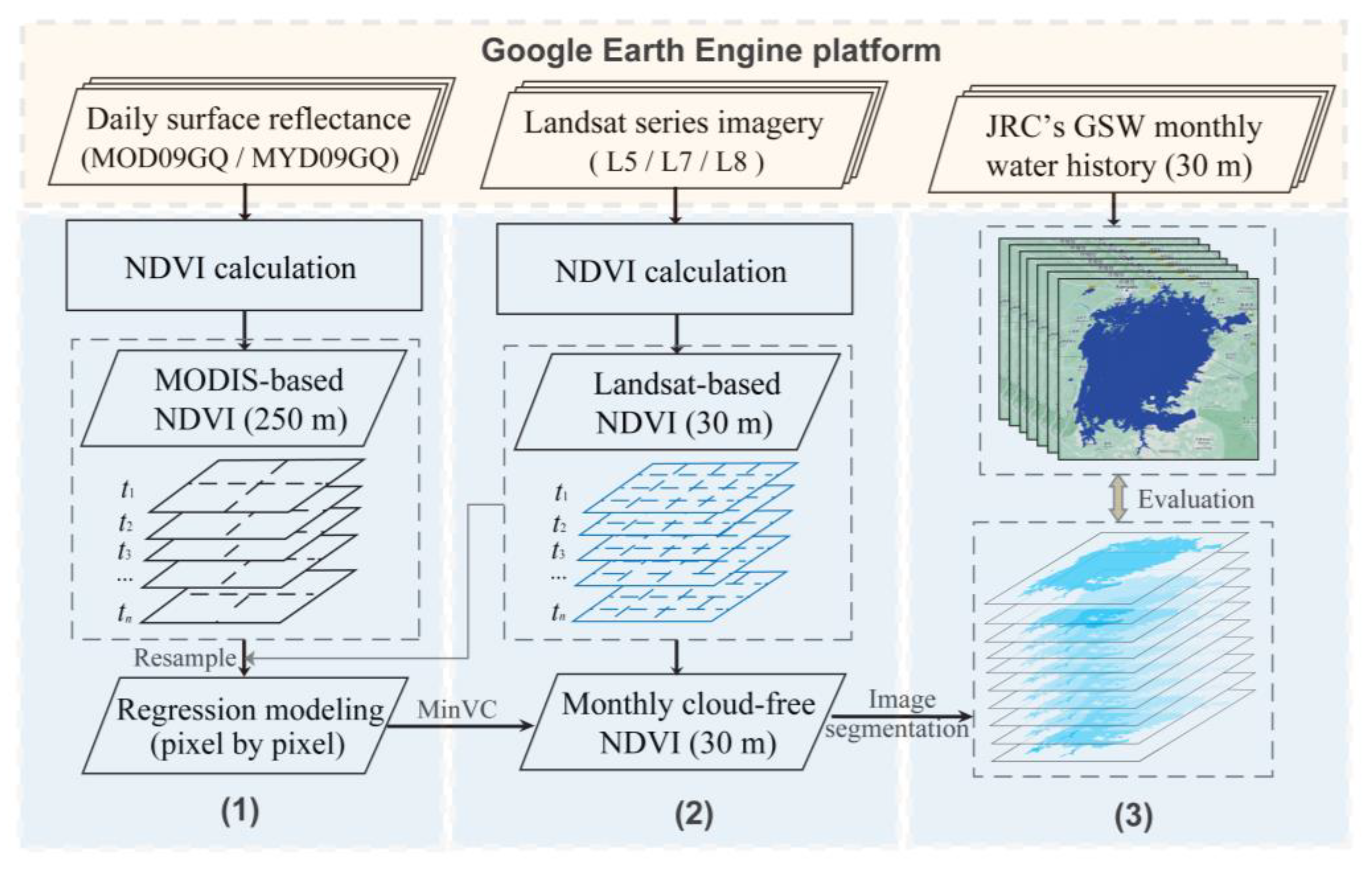
where ρ R e d and ρ N I R refer to the visible red and near-infrared bands of satellite images. Water bodies can be easily distinguished from background features with NDVI < 0 [47,48,49]. To generate SWE at a high spatio–temporal resolution, our MIFSWM method consists of three steps (Figure 2). First, MODIS NDVI was downscaled to Landsat resolution via a per-pixel regression-based method. Second, monthly Landsat-like cloud-free NDVIs were generated via the Minimum Value Composite (MinVC) algorithm. Finally, monthly water surfaces were delineated and validated. Each step is detailed below.

3.1. Downscaling MODIS NDVIs

In this study, a regression-based approach was used to downscale 250 m MODIS-NDVI images to 30 m resolution. The approach assumes that concurrent NDVI values from different sensors are highly correlated, and the correlations are consistent over the entire time [50]. The algorithm comprises the following four steps:
(a)
MODIS-NDVIs and Landsat-NDVIs were first calculated through Equation (1) based on the daily MOD09GQ/MYD09GQ and Landsat data with the same overpass time, respectively;
(b)
The MODIS-NDVIs (250 m) were consistently resampled to a spatial resolution of 30 m to match the Landsat-NDVI pixel size;
(c)
The resampled MODIS-NDVIs and Landsat-NDVIs were subsequently employed as independent and dependent variables for function regression to establish a downscaling model for each pixel. The model can be expressed as
NDVI i , j , t Landsat = a i , j NDVI i , j , t MODIS + b i , j
where NDVI i , j , t Landsat and NDVI i , j , t MODIS represent the value of Landsat-NDVI and resampled MODIS-NDVI at the pixel (i, j) and time t, respectively; a i , j and b i , j are fitting coefficients of the linear regression models.
(d)
Generating a daily time series of high-resolution NDVI images (30 m) using the constructed downscaling models.

3.2. Generating Monthly Cloud-Free NDVI Time Series

Clouds are common in hot and humid regions, which hiders the efficient detection of water bodies from satellite imagery [29]. To deal with this limitation, the MinVC algorithm was used to construct monthly cloud-free Landsat NDVIs. In the visible and near-infrared bands of MODIS and Landsat data, the spectral reflectance of clouds is spectrally flat, having NDVI values close to zero [51]. Water bodies generally exhibit large negative NDVI values and, if contaminated by clouds, show less but still negative NDVI values. Therefore, searching for the minimum NDVI value in a month would most likely correspond to water bodies. For a detailed explanation of this algorithm, please refer to our previous work [52].

3.3. Quantifying and Evaluating Surface Water Dynamics

In order to efficiently distinguish water and no-water features for the derived time series of NDVI images, the Otsu algorithm was used to delineate water surfaces [53]. The Otsu algorithm is one of the most popular dynamic threshold determination methods, which aims to separate water bodies from background features by maximizing the inter-class variance and minimizing intra-class variance in bimodal histograms of NDVI values [54]. To enhance water detection accuracy, we first divided NDVI images into equally sized blocks, on which the Otsu algorithm was used to derive local threshold values [55,56]. To evaluate the performance of our method, the Hydroweb water level data were correlated with water surface data. The SWE data were also compared with the JRC’s GSW data to examine their consistencies in describing water surface spatio–temporal dynamics in 2000–2020.

4. Results

4.1. Overall Performance of our Method

4.1.1. The Performance of Spatio–Temporal Resolution

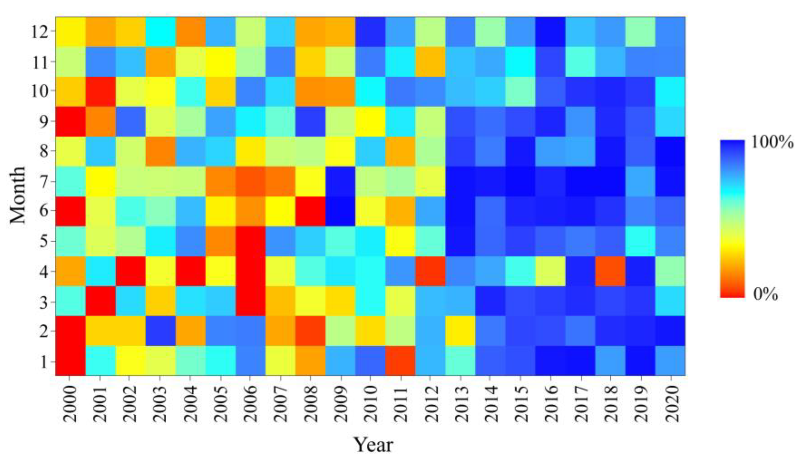
Based on the proposed MIFSWM method, we detected SWE dynamic series at a monthly time interval for Lake Victoria spanning a time period from 2000 to 2020. Figure 3 illustrates the comparison between monthly surface water surface area data derived from different results and the water level variability of Lake Victoria. Time series values marked with the green crosses (Figure 3a) and blue crosses (Figure 3b) are the monthly SWE results developed by JRC’s GSW and our method, respectively. To compare the reliability of different SWE results, altimeter water level time series were also produced, which are marked with orange circles. As shown in Figure 3a, the JRC’s GSW areas are overall low and vary considerably during 2000–2020. This was mainly caused by cloud contamination, which finally led to some gaps and invalid observations in JRC’s GSW results. Further examination (Figure 4) shows that the fraction of valid pixels is relatively low during our study period (only 93 valid observations), insufficient to capture SWE dynamics, especially during wet seasons (March–May) from 2000 to 2012. Our result, however, can well resolve the cloud contamination issues and improve the number of observations (Figure 3b). In particular, the MIFSWM-based SWE results have better temporal continuity and show quite high consistency with the altimeter water level time series, which will certainly facilitates the time series analysis.

4.1.2. Correlation with Water Level Series

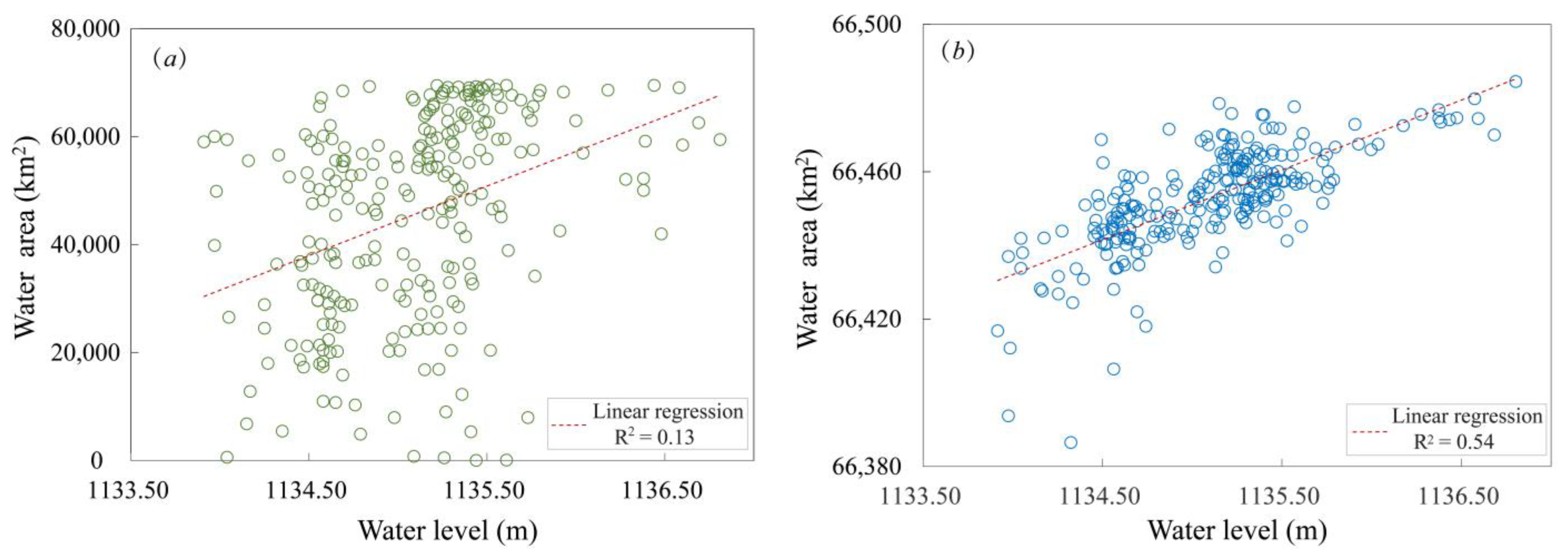
Figure 5 illustrates the scatter diagram between the monthly surface water area time series and the altimeter water level measurements from 2000 to 2020. As can be seen in Figure 5a, the linear least squares regression analysis resulted in low R2 values of 0.13 between the JRC’s GSW monthly water history records and altimeter water level time series, indicating that obvious gaps exist between the two datasets. However, as illustrated in Figure 5b, the monthly SWE data determined by our MIFSWM method are well-represented, which achieved highly significant correlations (R2 = 0.54) with altimeter water level time series. It suggested that the temporal variations of SWE data can be well captured using our method.

4.1.3. Visual Comparison of the SWE Results

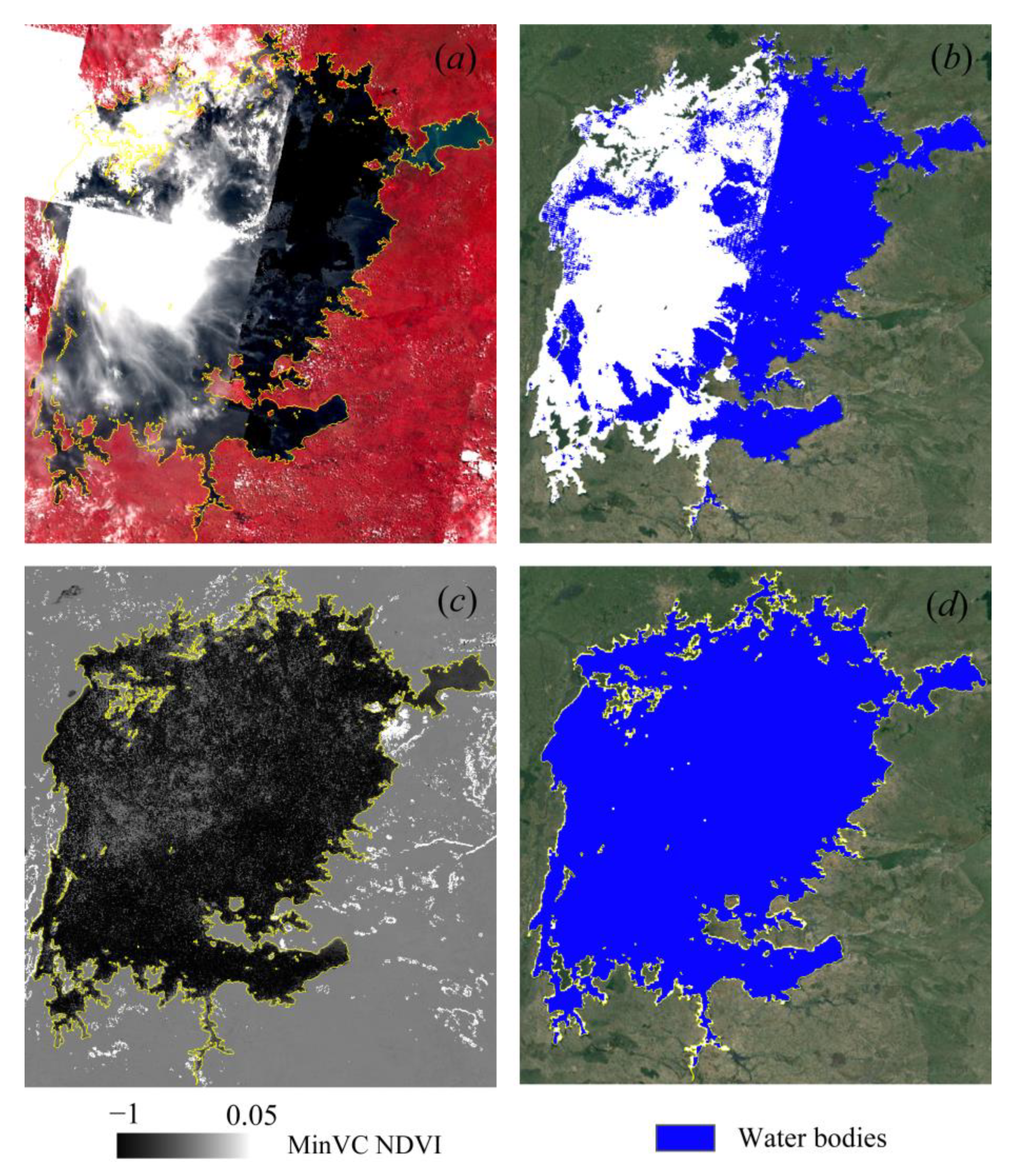
Visual inspection also corroborates the good performance of our method. Figure 6 presents a comparison between JRC’s GSW monthly water body map and MIFSWM-based SWE in April 2016 over Lake Victoria, which corresponds to the red frame in Figure 3. As revealed in Figure 6, the resultant surface water distribution derived from JRC’s GSW loses many spatial details and shows poor continuity (Figure 6b), probably due to the fact that it originally contains large spatial gaps caused by the cloud effects on Landsat imagery (Figure 6a). By contrast, the MinVC algorithm was adopted in monthly composite NDVI from daily surface reflectance data (Figure 6c), and clouds cover and cloud shadows were efficiently removed in MIFSWM-based surface water extent (Figure 6d). The resultant SWE of the MIFSWM method provides a continuous water body map and has better visual results. The visual comparison indicates that MIFSWM is a robust and efficient methodology for SWE detection, which allows better capturing of open surface water extent in cloudy conditions that are incompetent to be detected by JRC’s GSW monthly water history product.

4.2. Temporal Dynamics of SWE

4.2.1. Surface Water Dynamics at the Inter-Annual and Seasonal Scale

Figure 7 illustrates the time series of annual maximum, minimum, and mean surface water areas derived from our method in Lake Victoria. It is noticed that they all show similar fluctuation trends during the period from 2000 to 2020, which exhibits a pattern of an initial decline followed by an increase. From 2002 onwards, water areas were generally declining until they reached the lowest value of 66,386.57 km2 in 2006 (Figure 7), with an average descending rate of 8.79 km2 per year. While since 2006, on the whole, surface water areas have transitioned into a significant increasing trend year by year. The linear regression suggests that the inundation area was generally increasing at a rate of 5.51 km2 per year with several local fluctuations. These findings closely agree with the results of the previous study by Awange et al. in 2019 [9]. Furthermore, during the past 20 years, such inundation area fluctuations occurred in the extreme hydrological years of 2006 and 2020 were also well captured by our SWE results.
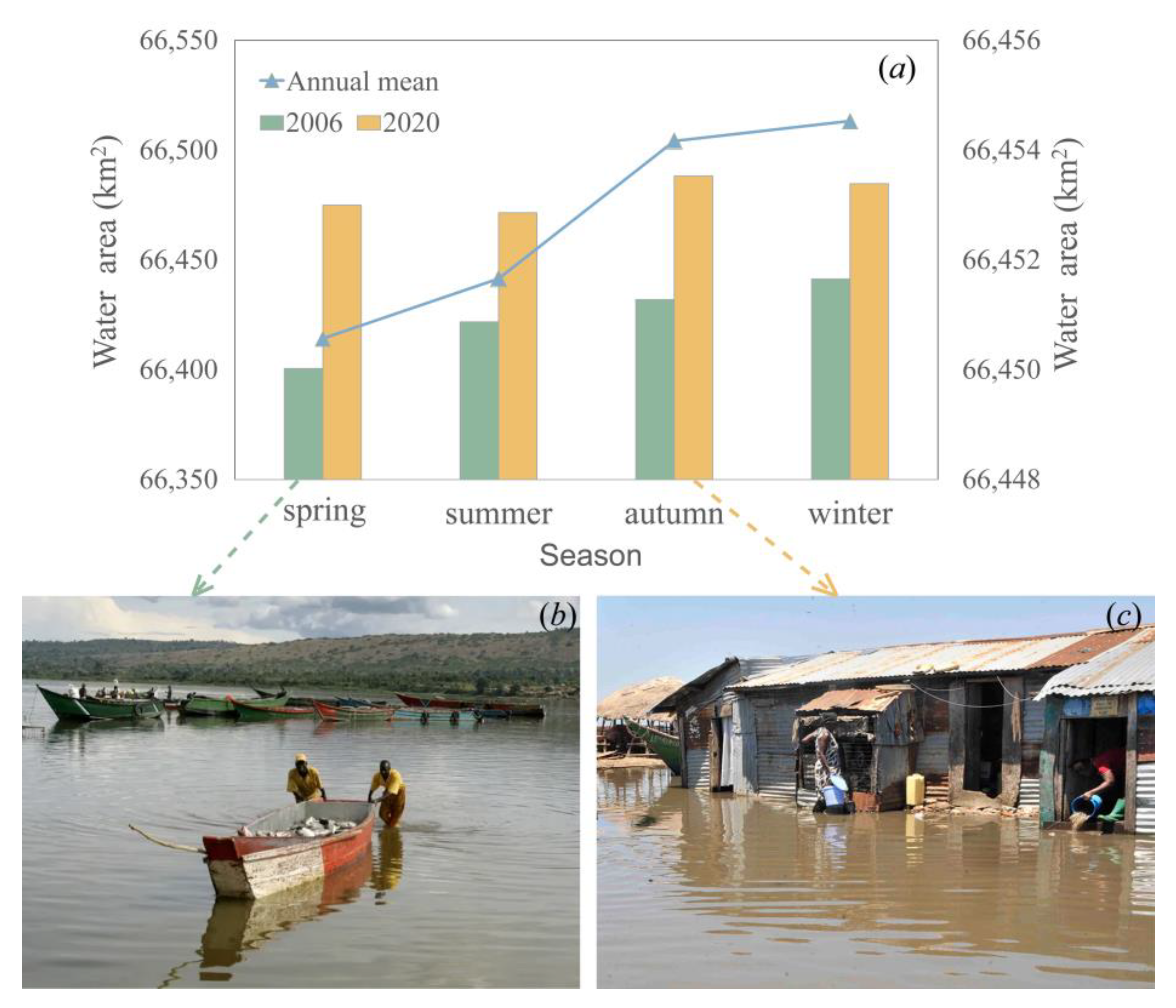
In regard to the average SWE of each month, a seasonal analysis of the surface water area was presented in Figure 8a. In the figure, a general seasonal variation pattern can be observed that the average SWE data are gradually increasing with the change of seasons. The largest lake area occurs in the southern hemisphere winter (June–August), and the smallest lake area occurs in spring (September–November). According to the previous studies of Nicholson [57] and Awange [12], most of Lake Victoria’s water supply comes from regional rainfall, and heavier rainfall at Lake Victoria is concentrated in March–June. Therefore, this seasonal variations in the lake area are generally consistent with local precipitation characteristics, which manifests a general seasonality of dry in spring and wet in winter. Particularly in the spring of 2006 and autumn of 2020, Lake Victoria witnessed intense episodes of drought and flooding events, respectively (Figure 8b,c), which have posed significant impacts on the lake’s shoreline communities in some hotspot regions [7,10].

4.2.2. Extreme SWEs in 2006 and 2020

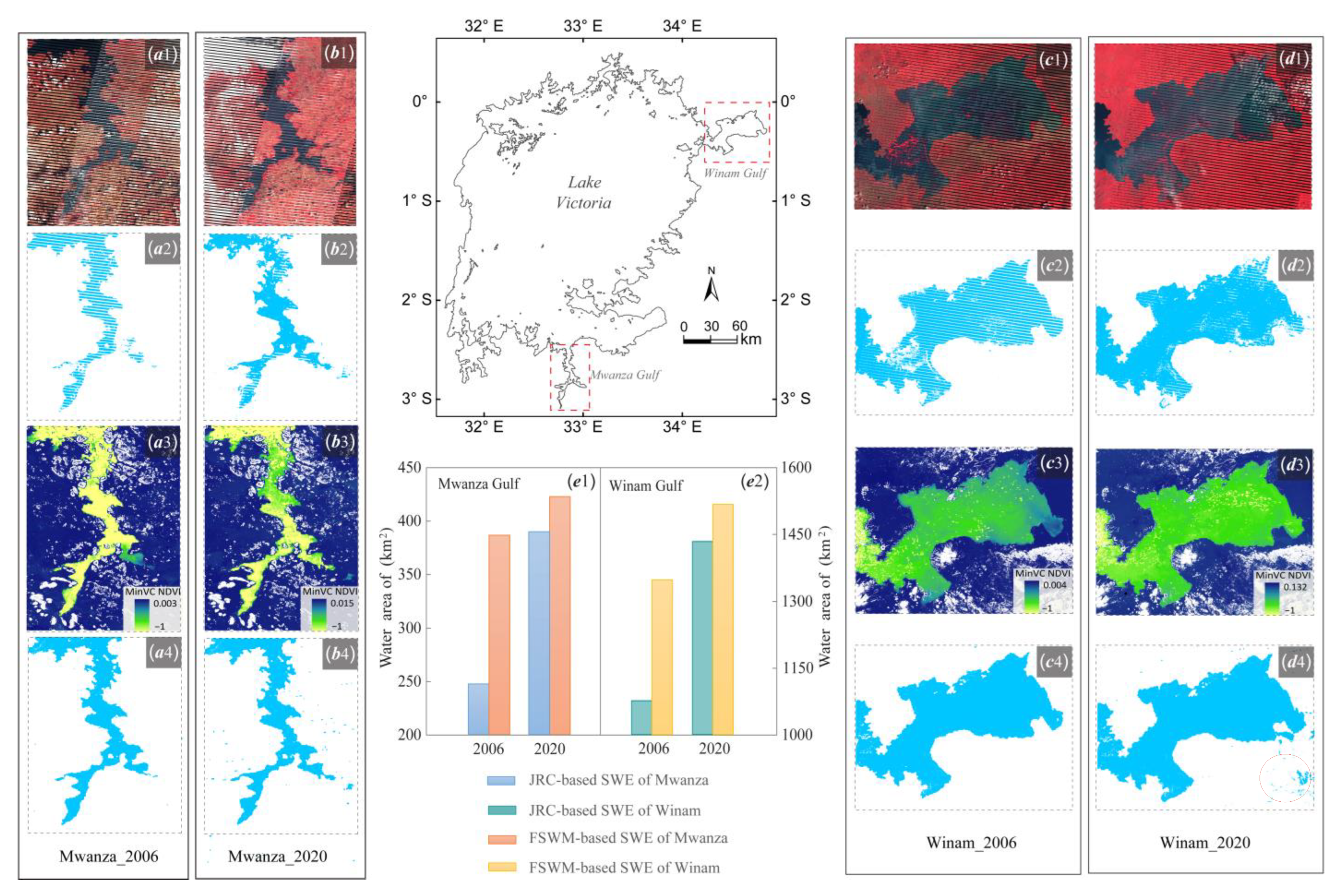
To determine the ability of our SWE result to capture extreme inundation conditions in 2006 and 2020, we further focused on two detailed examples of surface water mapping in Mwanza Gulf (in the south) and Winam Gulf (in the northeast) (Figure 9). Figure 9 shows two enlarged mapping results in the southern Mwanza Gulf and the northeastern Winam Gulf. It was found that both the JRC’s GSW dataset and our result reflect extreme inundation conditions, i.e., shrunk lake area in 2006 and expanded lake area in 2020. However, the changes are not accurately reflected by JRC’s GSW dataset. In the Winam Gulf, the lake area increased by 32.82% (from 1072.77 km2 to 1424.82 km2) as detected by JRC’s GSW, whereas it only increased by 12.22% (from 1332.06 km2 to 1494.89 km2) based on our method (Figure 9(e1,e2)). The change rate of JRC’s GSW seems higher, but the value is spurious. Further inspection in Figure 9(a2–d2) shows that JRC’s GSW loses spatial details, leading to consistent underestimation of lake areas. There are two possible reasons for this phenomenon. For one thing, the resultant surface water maps of the JRC’s GSW show poor continuity, which originally contained gaps due to sporadic clouds cover and linear strips from Landsat images, making it easy to lose spatial details. For another, Winam Gulf is characterized by extensive coastal floating vegetation or wetland floodplains [58]. These inundation conditions are difficult to be detected from the JRC’s GSW because the spectral signature is confused by vegetation. By contrast, as shown in Figure 9(c4,d4), our method is more robust and could capture this detailed inundation well owing to the available cloud-free MinVC NDVI, especially in the southeastern shore of Winam Gulf (highlighted by red circles in Figure 9(d4)). It not only expresses relatively continuous water maps with better visual results but also attains a higher performance regardless of the weather conditions, which could provide a real representation of water safety and help to guide regional water resource management such as water supply, fisheries, and navigation.

5. Conclusions and Discussion

5.1. Conclusions

In this study, we developed a MIFSWM methodology to derive monthly 30 m SWE time series over Lake Victoria from 2000 to 2022. The 250 m MODIS NDVI images were first reconciled with the 30 m Landsat NDVI images, creating high-resolution daily NDVI time series. Monthly cloud-free NDVI series were then composited via the MinVC algorithm and were finally segmented to generate seamless SWEs. The result was evaluated based on a satellite altimetry-based water level dataset and a state-of-the-art SWE product. Our result is superior to the JRC’s GSW dataset, which underestimates lake areas due to several gap issues. Moreover, it is more consistent with the water level series. Based on the new dataset, we re-examined the long-term and seasonal SWE dynamics of Lake Victoria. In the last 20 years, a significant changing pattern of an initial decline followed by an increase was found in inundation areas. The annual mean inundation area showed a significant declining trend from 2002 to 2006 (−8.79 km2·a−1). The trend was overturned in 2006, when a significant increasing trend (5.51 km2·a−1) was observed. The new dataset can successfully capture extreme inundation conditions in two hotspot gulfs, further corroborating the effectiveness of our method.

5.2. Future Outlook and Implications

To our knowledge, the MIFSWM method offers the first high-resolution, seamless surface water maps at a monthly scale in Lake Victoria. Compared with the existing SWE dataset, it can provide reliable descriptions of spatio–temporal dynamics of water bodies. We believe this work provides several important implications for both managerial practice and future research.
Firstly, as the largest freshwater lake in Africa, Lake Victoria supports the livelihood of more than 30 million people living around it. It modulates regional climate and plays a crucial role in regional sustainable development and biodiversity conservation, but it is also prone to hydrological extremes [59,60]. Fortunately, time series of inundation information permits effective monitoring of the long-term variations in SWE, including some hotspot gulfs and even small water bodies. It would benefit the water safety management program to minimize casualties and property damage. The long monitoring information reported here may also potentially contribute to a more comprehensive understanding of regional hydrological and biogeochemical processes. It would be helpful to provide new insights for tracking and quantifying climate change and human influences on regional SWE variability.
Secondly, our proposed methodology shows obvious superiority compared with some recent methods of surface water dynamic monitoring using Landsat and MODIS archives. Although some methodologies have been presented for exploring surface water dynamics, most of the current products are discontinuous in space or time. Our method makes the best of MODIS and Landsat data to develop a collaborative framework for data fusion and cloud removal. In this framework, an NDVI downscaling strategy and MinVC algorithm are combined to efficiently overcome data gaps and coarse-resolution problems, which is our key innovation. What is more, the MIFSWM methodology is implemented on the GEE platform, where daily MODIS data, Landsat, and Sentinel-2 data are available worldwide. It can be easily extended to other high-resolution images and to other regions. It may prove as a useful tool to provide a unique opportunity for continuous and reliable surface water mapping. Besides these practical contributions, the proposed methodology may have limitations to be addressed in the future. It should be noted that NDVI is the most common index to identify water body information. However, the land surface in water bodies’ environment is complex; it also faces problems of distinguishing shadows, buildings, or dark soil from water. Thus, the algorithms used to effectively remove shadows should be further improved to generate a more accurate SWE dataset.

Author Contributions

Conceptualization, G.W. and Y.L. (Yuanbo Liu); methodology, G.W. and X.F.; software, C.C. and H.N.; writing—review and editing, G.W.; supervision, Y.L. (Yongwei Liu) and X.F. All authors have read and agreed to the published version of the manuscript.

Funding

This research was jointly supported by the National Key Research and Development Program of China (2018YFE0105900), the National Natural Science Foundation of China (41871354, 51839011), the Key Deployment Projects of Sino-Africa Joint Research Center, Chinese Academy of Sciences (SAJC202106), and the International Collaboration Program of Chinese Academy of Science (151542KYSB20200015).

Data Availability Statement

The data presented in this study are available on request from the corresponding author.

Conflicts of Interest

The authors declare no conflict of interest.

References

  1. Beverly, E.J.; White, J.D.; Peppe, D.J.; Faith, J.T.; Blegen, N.; Tryon, C.A. Rapid Pleistocene desiccation and the future of Africa’s Lake Victoria. Earth Planet. Sci. Lett. 2020, 530, 115883. [Google Scholar] [CrossRef]
  2. Olokotum, M.; Mitroi, V.; Troussellier, M.; Semyaloa, R.; Bernarde, C.; Montuelle, B.; Okello, W.; Quiblier, C.; Humbert, J.-F. A review of the socioecological causes and consequences of cyanobacterial blooms in Lake Victoria. Harmful Algae 2020, 96, 101829. [Google Scholar] [CrossRef] [PubMed]
  3. Swenson, S.; Wahr, J. Monitoring the water balance of Lake Victoria, East Africa, from space. J. Hydrol. 2009, 370, 163–176. [Google Scholar] [CrossRef]
  4. Liu, Y.; Wu, G.; Fan, X.; Gan, G.; Wang, W.; Liu, Y. Hydrological impacts of land use/cover changes in the Lake Victoria basin. Ecol. Indic. 2022, 145, 109580. [Google Scholar] [CrossRef]
  5. Shen, Q.; Friese, K.; Gao, Q.; Yu, C.; Kimirei, I.A.; Kishe-Machumu, M.A.; Zhang, L.; Wu, G.P.; Liu, Y.B.; Zhang, J.Q.; et al. Status and changes of water quality in typical near-city zones of three East African Great Lakes in Tanzania. Environ. Sci. Pollut. Res. 2022, 29, 34105–34118. [Google Scholar] [CrossRef]
  6. Kipyegon, B.D.; Wehn, U.; van der Zaag, P. Lake Victoria water levels declining (2000–2006): The role of absent and uncertain data in a transboundary water controversy. Water Int. 2022, 1–13. [Google Scholar] [CrossRef]
  7. Awange, J.; Anyah, R.; Agola, N.; Forootan, E.; Omondi, P. Potential impacts of climate and environmental change on the stored water of Lake Victoria Basin and economic implications. Water Resour. Res. 2013, 49, 8160–8173. [Google Scholar] [CrossRef] [Green Version]
  8. Okotto-Okotto, J.; Raburu, P.O.; Obiero, K.O.; Obwoyere, G.O.; Mironga, J.M.; Okotto, L.G.; Raburu, E.A. Spatio-temporal impacts of Lake Victoria water level recession on the fringing Nyando Wetland, Kenya. Wetlands 2018, 38, 1107–1119. [Google Scholar] [CrossRef]
  9. Awange, J.L.; Saleem, A.; Sukhadiya, R.; Ouma, Y.O.; Hu, K. Physical dynamics of Lake Victoria over the past 34 years (1984–2018): Is the lake dying? Sci. Total Environ. 2019, 658, 199–218. [Google Scholar] [CrossRef]
  10. Khaki, M.; Awange, J. The 2019–2020 Rise in Lake Victoria Monitored from Space: Exploiting the State-of-the-Art GRACE-FO and the Newly Released ERA-5 Reanalysis Products. Sensors 2021, 21, 4304. [Google Scholar] [CrossRef]
  11. Khan, S.I.; Hong, Y.; Wang, J.; Yilmaz, K.K.; Gourley, J.J.; Adler, R.F.; Brakenridge, G.R.; Policelli, F.; Habib, S.; Irwin, D. Satellite Remote Sensing and Hydrologic Modeling for Flood Inundation Mapping in Lake Victoria Basin: Implications for Hydrologic Prediction in Ungauged Basins. IEEE Trans. Geosci. Remote Sens. 2011, 49, 85–95. [Google Scholar] [CrossRef] [Green Version]
  12. Awange, J. Lake Victoria Monitored from Space; Springer: Berlin/Heidelberg, Germany, 2021. [Google Scholar]
  13. Chawla, I.; Karthikeyan, L.; Mishra, A.K. A review of remote sensing applications for water security: Quantity, quality, and extremes. J. Hydrol. 2020, 585, 124826. [Google Scholar] [CrossRef]
  14. Yang, X.; Wang, N.; Chen, A.A.; He, J.; Hua, T.; Qie, Y. Changes in area and water volume of the Aral Sea in the arid Central Asia over the period of 1960–2018 and their causes. CATENA 2020, 191, 104566. [Google Scholar] [CrossRef]
  15. Huang, C.; Chen, Y.; Zhang, S.; Wu, J. Detecting, extracting, and monitoring surface water from space using optical sensors: A review. Rev. Geophys. 2018, 56, 333–360. [Google Scholar] [CrossRef]
  16. Gao, H. Satellite remote sensing of large lakes and reservoirs: From elevation and area to storage. Wiley Interdiscip. Rev. Water 2015, 2, 147–157. [Google Scholar] [CrossRef]
  17. Wu, G.; Xiao, X.; Liu, Y. Satellite-Based Surface Water Storage Estimation: Its History, Current Status, and Future Prospects. IEEE Geosci. Remote Sens. Mag. 2022, 10, 10–31. [Google Scholar] [CrossRef]
  18. Tong, X.; Pan, H.; Xie, H.; Xu, X.; Li, F.; Chen, L.; Luo, X.; Liu, S.; Chen, P.; Jin, Y. Estimating water volume variations in Lake Victoria over the past 22 years using multi-mission altimetry and remotely sensed images. Remote Sens. Environ. 2016, 187, 400–413. [Google Scholar] [CrossRef]
  19. Lin, Y.; Li, X.; Zhang, T.; Chao, N.; Yu, J.; Cai, J.; Sneeuw, N. Water Volume Variations Estimation and Analysis Using Multisource Satellite Data: A Case Study of Lake Victoria. Remote Sens. 2020, 12, 3052. [Google Scholar] [CrossRef]
  20. Pekel, J.F.; Cottam, A.; Gorelick, N.; Belward, A.S. High-resolution mapping of global surface water and its long-term changes. Nature 2016, 540, 418–422. [Google Scholar] [CrossRef]
  21. Klein, I.; Gessner, U.; Dietz, A.J.; Kuenzer, C. Global WaterPack–A 250 m resolution dataset revealing the daily dynamics of global inland water bodies. Remote Sens. Environ. 2017, 198, 345–362. [Google Scholar] [CrossRef]
  22. Feng, M.; Sexton, J.O.; Channan, S.; Townshend, J.R. A global, high-resolution (30-m) inland water body dataset for 2000: First results of a topographic–spectral classification algorithm. Int. J. Digit. Earth 2016, 9, 113–133. [Google Scholar] [CrossRef] [Green Version]
  23. Ling, F.; Li, X.; Foody, G.M.; Boyd, D.; Ge, Y.; Li, X.; Du, Y. Monitoring Surface Water Area Variations of Reservoirs Using Daily MODIS Images by Exploring Sub-Pixel Information. ISPRS J. Photogramm. Remote Sens. 2020, 168, 141–152. [Google Scholar] [CrossRef]
  24. Yao, F.; Wang, J.; Wang, C.; Crétaux, J. Constructing long-term high-frequency time series of global lake and reservoir areas using Landsat imagery. Remote Sens. Environ. 2019, 232, 111210. [Google Scholar] [CrossRef]
  25. Li, L.; Skidmore, A.; Vrieling, A.; Wang, T. A new dense 18-year time series of surface water fraction estimates from MODIS for the Mediterranean region. Hydrol. Earth Syst. Sci. 2019, 23, 3037–3056. [Google Scholar] [CrossRef] [Green Version]
  26. Li, L.; Vrieling, A.; Skidmore, A.; Wang, T. Evaluation of a new 18-year MODIS-derived surface water fraction dataset for constructing Mediterranean wetland open surface water dynamics. J. Hydrol. 2020, 587, 124956. [Google Scholar] [CrossRef]
  27. Li, Y.; Gao, H.; Zhao, G.; Tseng, K.H. A high-resolution bathymetry dataset for global reservoirs using multi-source satellite imagery and altimetry. Remote Sens. Environ. 2020, 244, 111831. [Google Scholar] [CrossRef]
  28. Bai, B.; Tan, Y.; Zhou, K.; Donchyts, G.; Haag, A.; Weerts, A.H. Time-series surface water gap filling based on spatiotemporal neighbourhood similarity. Int. J. Appl. Earth Obs. Geoinf. 2022, 112, 102882. [Google Scholar] [CrossRef]
  29. Zhu, X.; Helmer, E.H. An automatic method for screening clouds and cloud shadows in optical satellite image time series in cloudy regions. Remote Sens. Environ. 2018, 214, 135–153. [Google Scholar] [CrossRef]
  30. Yang, X.; Qin, Q.; Yésou, H.; Ledauphin, T.; Koehl, M.; Grussenmeyer, P.; Zhu, Z. Monthly Estimation of the Surface Water Extent in France at a 10-m Resolution Using Sentinel-2 Data. Remote Sens. Environ. 2020, 244, 111803. [Google Scholar] [CrossRef]
  31. Li, X.; Ling, F.; Cai, X.; Ge, Y.; Li, X.; Yin, Z.; Shang, C.; Jia, X.; Du, Y. Mapping water bodies under cloud cover using remotely sensed optical images and a spatiotemporal dependence model. Int. J. Appl. Earth Obs. Geoinf. 2021, 103, 102470. [Google Scholar] [CrossRef]
  32. Gao, F.; Masek, J.; Schwaller, M.; Hall, F. On the Blending of the Landsat and MODIS Surface Reflectance: Predicting Daily Landsat Surface Reflectance. IEEE Trans. Geosci. Remote Sens. 2006, 44, 2207–2218. [Google Scholar]
  33. Hilker, T.; Wulder, M.A.; Coops, N.C.; Linke, J.; McDermid, G.; Masek, J.G.; Gao, F.; White, J.C. A new data fusion model for high spatial-and temporal-resolution mapping of forest disturbance based on Landsat and MODIS. Remote Sens. Environ. 2009, 113, 1613–1627. [Google Scholar] [CrossRef]
  34. Zhu, X.; Cai, F.; Tian, J.; Williams, T.K.A. Spatiotemporal Fusion of Multi-source Remote Sensing Data: Literature Survey, Taxonomy, Principles, Applications, and Future Directions. Remote Sens. 2018, 10, 527. [Google Scholar] [CrossRef] [Green Version]
  35. Li, X.; Jia, X.; Yin, Z.; Du, Y.; Ling, F. Integrating MODIS and Landsat imagery to monitor the small water area variations of reservoirs. Sci. Remote. Sens. 2022, 5, 100045. [Google Scholar] [CrossRef]
  36. Wang, Q.; Zhang, Y.; Onojeghuo, A.O.; Zhu, X.; Atkinson, P.M. Enhancing Spatio–temporal Fusion of MODIS and Landsat Data by Incorporating 250 m MODIS Data. IEEE J. Sel. Top. Appl. Earth Obs. Remote Sens. 2017, 10, 4116–4123. [Google Scholar] [CrossRef] [Green Version]
  37. Cheng, Q.; Shen, H.; Zhang, L.; Yuan, Q.; Zeng, C. Cloud removal for remotely sensed images by similar pixel replacement guided with a spatio–temporal MRF model. ISPRS J. Photogramm. Remote Sens. 2014, 92, 54–68. [Google Scholar]
  38. Zhang, X.; Qiu, Z.; Peng, C.; Ye, P. Removing cloud cover interference from Sentinel-2 imagery in Google Earth Engine by fusing Sentinel-1 SAR data with a CNN model. Int. J. Remote Sens. 2022, 43, 132–147. [Google Scholar] [CrossRef]
  39. Papa, F.; Crétaux, J.-F.; Grippa, M.; Robert, E.; Trigg, M.; Tshimanga, R.M.; Kitambo, B.; Paris, A.; Carr, A.; Fleischmann, A.S. Water Resources in Africa under Global Change: Monitoring Surface Waters from Space. Surv. Geophys. 2023, 44, 43–93. [Google Scholar] [CrossRef]
  40. Paul, S.; Oppelstrup, J.; Thunvik, R.; Magero, J.M.; Ddumba Walakira, D.; Cvetkovic, V. Bathymetry development and flow analyses using two-dimensional numerical modeling approach for Lake Victoria. Fluids 2019, 4, 182. [Google Scholar] [CrossRef] [Green Version]
  41. Ngoma, H.; Wang, W.; Ojara, M.; Ayugi, B. Assessing current and future spatiotemporal precipitation variability and trends over Uganda, East Africa, based on CHIRPS and regional climate model datasets. Meteorol. Atmos. Phys. 2021, 133, 823–843. [Google Scholar] [CrossRef]
  42. Hao, Y.; Baik, J.; Fred, S.; Choi, M. Comparative Analysis of Two Drought Indices in the Calculation of Drought Recovery Time and Implications on Drought Assessment: East Africa’s Lake Victoria Basin. Stoch. Environ. Res. Risk Assess. 2021, 36, 1943–1958. [Google Scholar] [CrossRef]
  43. United States Geological Survey (USGS). The Website of the Land Processes Distributed Active Archive Center (LP DAAC). Available online: https://lpdaac.usgs.gov/products/mod09gqv061 (accessed on 19 March 2023).
  44. Crétaux, J.-F.; Jelinski, W.; Calmant, S.; Kouraev, A.; Vuglinski, V.; Bergé-Nguyen, M.; Gennero, M.-C.; Nino, F.; Del Rio, R.A.; Cazenave, A. SOLS: A lake database to monitor in the Near Real Time water level and storage variations from remote sensing data. Adv. Space Res. 2011, 47, 1497–1507. [Google Scholar] [CrossRef]
  45. Gorelick, N.; Hancher, M.; Dixon, M.; Ilyushchenko, S.; Thau, D.; Moore, R. Google Earth Engine: Planetary-scale geospatial analysis for everyone. Remote Sens. Environ. 2017, 202, 18–27. [Google Scholar] [CrossRef]
  46. Pettorelli, N.; Vik, J.O.; Mysterud, A.; Gaillard, J.M.; Tucker, C.J.; Stenseth, N.C. Using the satellite–derived NDVI to assess ecological responses to environmental change. Trend. Ecol. Evol. 2005, 20, 503–510. [Google Scholar] [CrossRef]
  47. Wang, J.; Ding, J.; Li, G.; Liang, J.; Yu, D.; Aishan, T.; Zhang, F.; Yang, J.; Abulimiti, A.; Liu, J. Dynamic detection of water surface area of Ebinur Lake using multi-source satellite data (Landsat and Sentinel-1A) and its responses to changing environment. Catena 2019, 177, 189–201. [Google Scholar] [CrossRef]
  48. Ahamed, A.; Bolten, J.D. A MODIS-based automated flood monitoring system for southeast asia. Int. J. Appl. Earth Obs. Geoinf. 2017, 61, 104–117. [Google Scholar] [CrossRef] [Green Version]
  49. Han, Q.; Niu, Z. Construction of the long-term global surface water extent dataset based on water-NDVI spatio–temporal parameter set. Remote Sens. 2020, 12, 2675. [Google Scholar] [CrossRef]
  50. Wu, G.; Liu, Y. Downscaling Surface Water Inundation from Coarse Data to Fine-Scale Resolution: Methodology and Accuracy Assessment. Remote Sens. 2015, 7, 15989–16003. [Google Scholar] [CrossRef] [Green Version]
  51. Istomina, L.; Marks, H.; Huntemann, M.; Heygster, G.; Spreen, G. Improved cloud detection over sea ice and snow during Arctic summer using MERIS data. Atmos. Meas. Technol. 2020, 13, 6459–6472. [Google Scholar] [CrossRef]
  52. Fan, X.; Liu, Y.; Wu, G.; Zhao, X. Compositing the Minimum NDVI for Daily Water Surface Mapping. Remote Sens. 2020, 12, 700. [Google Scholar] [CrossRef] [Green Version]
  53. Otsu, N. A threshold selection method from gray-level histograms. IEEE Trans. Syst. Man Cybern. 1979, 9, 62–66. [Google Scholar] [CrossRef] [Green Version]
  54. Zhang, G.; Zheng, G.; Gao, Y.; Xiang, Y.; Lei, Y.; Li, J. Automated Water Classification in the Tibetan Plateau Using Chinese GF-1 WFV Data. Photogramm. Eng. Remote Sens. 2017, 83, 509–519. [Google Scholar] [CrossRef]
  55. Ludwig, C.; Walli, A.; Schleicher, C.; Weichselbaum, J.; Riffler, M. A highly automated algorithm for wetland detection using multi-temporal optical satellite data. Remote Sens. Environ. 2019, 224, 333–351. [Google Scholar] [CrossRef]
  56. Fu, H.; Shen, Y.; Liu, J.; He, G.; Chen, J.; Liu, P.; Qian, J.; Li, J. Cloud detection for FY meteorology satellite based on ensemble thresholds and random forests approach. Remote Sens. 2019, 11, 44. [Google Scholar] [CrossRef] [Green Version]
  57. Nicholson, S.E. Climate and climatic variability of rainfall over eastern Africa. Rev. Geophys. 2017, 55, 590–635. [Google Scholar] [CrossRef] [Green Version]
  58. Fusilli, L.; Collins, M.O.; Laneve, G.; Palombo, A.; Pignatti, S.; Santini, F. Assessment of the abnormal growth of floating macrophytes in Winam Gulf (Kenya) by using MODIS imagery time series. Int. J. Appl. Earth Obs. Geoinf. 2013, 20, 33–41. [Google Scholar] [CrossRef]
  59. Khan, S.I.; Adhikari, P.; Hong, Y.; Vergara, H.; F Adler, R.; Policelli, F.; Irwin, D.; Korme, T.; Okello, L. Hydroclimatology of Lake Victoria region using hydrologic model and satellite remote sensing data. Hydrol. Earth Syst. Sci. 2011, 15, 107–117. [Google Scholar] [CrossRef] [Green Version]
  60. Mugo, R.; Waswa, R.; Nyaga, J.W.; Ndubi, A.; Adams, E.C.; Flores-Anderson, A.I. Quantifying Land Use Land Cover Changes in the Lake Victoria Basin Using Satellite Remote Sensing: The Trends and Drivers between 1985 and 2014. Remote Sens. 2020, 12, 2829. [Google Scholar] [CrossRef]
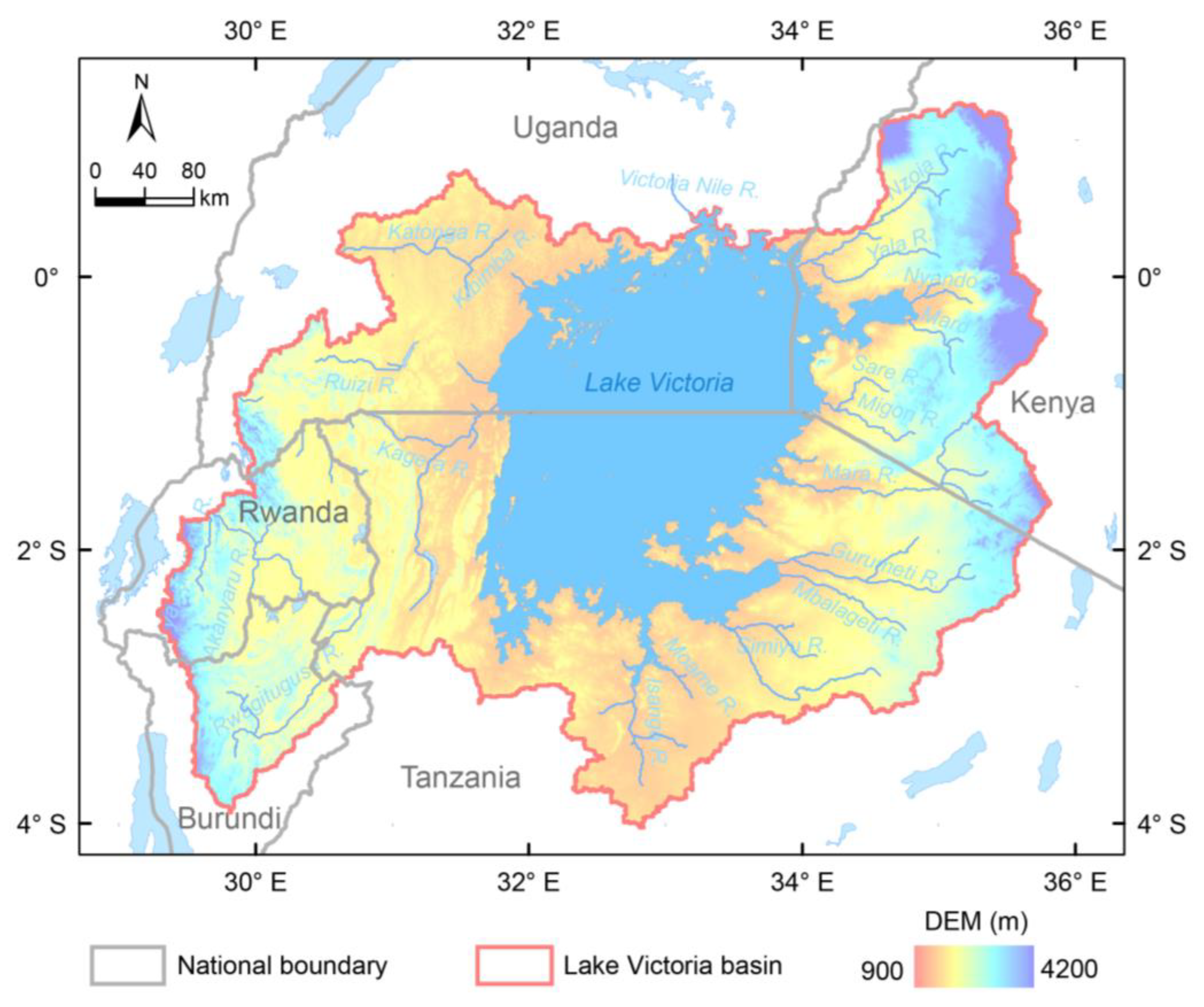
Figure 1. Geographical location of Lake Victoria.
Remotesensing 15 03500 g001
Figure 2. Schematic workflow of the proposed MIFSWM approach.
Remotesensing 15 03500 g002
Figure 3. Comparison of water level series (orange dots) with (a) JRC’s GSW data (green crosses) and (b) our SWE results (blue crosses) during the period of 2000–2020. The red box indicates the derived water area comparison in April 2016 between the results of JRC’s GSW and our SWE result.
Remotesensing 15 03500 g003
Figure 4. The fraction of valid pixels in monthly Landsat images between 2000 and 2020.
Remotesensing 15 03500 g004
Figure 5. Scatter diagrams between water level data and (a) monthly JRC’s GSW SWE data (green dots) and (b) our SWE results (blue dots), respectively.
Remotesensing 15 03500 g005
Figure 6. Comparison of JRC’s GSW SWE and our SWE result in April 2016. (a) False color composite of Landsat image; (b) JRC’s GSW SWE; (c) cloud-free MinVC NDVI; (d) our SWE result.
Remotesensing 15 03500 g006
Figure 7. Time series of annual maximum, minimum, and mean surface water areas from 2000 to 2020. The regression line (shown as a dotted line) between the annual mean area and time exhibits a pattern of an initial decline followed by an increase.
Remotesensing 15 03500 g007
Figure 8. Seasonal SWE variations of Lake Victoria (a). Subfigure (b) shows low SWE preventing fishermen from docking fishing boats in the spring of 2006 (quoted from: https://www.ocala.com/story/news/2006/12/10/lake-victorias-levels-drop-puts-african-nations-at-risk/31177621007/ (accessed on 28 June 2023). Subfigure (c) shows shoreline communities flooded by large SWE in the autumn of 2020 (quoted from: https://eos.org/articles/heavy-rains-human-activity-and-rising-waters-at-lake-victoria (accessed on 28 June 2023).
Remotesensing 15 03500 g008
Figure 9. Visual interpretation and comparison of surface water mapping under extreme inundation conditions for JRC- and MIFSWM-based results. (a1d1) are the false-color composite of the Landsat imagery of Mwanza Gulf and Winam Gulf in November 2006 and November 2020, respectively. (a2d2) are JRC-based surface water maps derived from (a1d1). (a3d3,a4d4) show the cloud-free MinVC NDVI and MIFSWM-based inundation maps corresponding to each period. The histogram (e1,e2) displays the surface water area statistics estimated by JRC’s GSW and our MIFSWM between 2006 and 2020.
Remotesensing 15 03500 g009
Table 1. Summary of the datasets used in this study.
Disclaimer/Publisher’s Note: The statements, opinions and data contained in all publications are solely those of the individual author(s) and contributor(s) and not of MDPI and/or the editor(s). MDPI and/or the editor(s) disclaim responsibility for any injury to people or property resulting from any ideas, methods, instructions or products referred to in the content.