Abstract
Fine-grained classification of ship targets is an important task in remote sensing, having numerous applications in military reconnaissance and sea surveillance. Due to the influence of various imaging factors, ship targets in remote sensing images have considerable inter-class similarity and intra-class difference, which brings significant challenges to fine-grained classification. In response, we developed a contrastive learning network based on causal attention (C2Net) to improve the model’s fine-grained identification ability from local details. The asynchronous feature learning mode of “decoupling + aggregation” is adopted to reduce the mutual influence between local features and improve the quality of local features. In the decoupling stage, the feature vectors of each part of the ship targets are de-correlated using a decoupling function to prevent feature adhesion. Considering the possibility of false associations between results and features, the decoupled part is designed based on the counterfactual causal attention network to enhance the model’s predictive logic. In the aggregation stage, the local attention weight learned in the decoupling stage is used to carry out feature fusion on the trunk feature weight. Then, the proposed feature re-association module is used to re-associate and integrate the target local information contained in the fusion feature to obtain the target feature vector. Finally, the aggregation function is used to complete the clustering process of the target feature vectors and fine-grained classification is realized. Using two large-scale datasets, the experimental results show that the proposed C2Net method had better fine-grained classification than other methods.
1. Introduction
Ship is an important type of remote sensing target and its classification and recognition are of great significance to both the military and civilian fields. In the military field, ship target identification is important in the deployment of maritime forces for reconnaissance and provides important intelligence support for command and decision-making. In civilian applications, accurate ship type identification plays a vital role in maritime rescue, fishery management, and anti-smuggling. Therefore, ship target recognition has many application prospects and values.
Ship target classification tasks can be roughly divided into target-level, coarse-grained, and fine-grained. Research on target-level classification [1,2] mainly focuses on distinguishing the target and background, which is essentially a binary task. Coarse-grained classification [3] focuses on categories with significant differences, such as aircraft carriers, warships, and merchant ships. Fine-grained classification [4,5,6,7,8] further distinguishes each category into sub-categories. Inter-class similarity and intra-class difference caused by different imaging factors (e.g., illumination, perspective change, and deformation) can make the fine-grained classification task more challenging, as shown in Figure 1. Therefore, the high-precision, fine-grained classification of ship targets has become a research hotspot in computer vision.
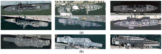
Figure 1.
(a) Inter-class similarity: Destroyer (first row), Frigate (second row); (b) Intra-class difference: aircraft carrier.
Some strongly supervised methods use target local location tags [9] or key location tags [10] to train the model’s localization and feature extraction ability for local areas. For example, Zhang et al. [11] used additional label information to train attributes to guide branches to achieve multi-level feature fusion. Chen et al. [12] conducted ship recognition by training a multi-level feature extraction network. This strong supervision method can improve the fine-grained classification effect. However, its high training information conditions, which require the local annotation of the dataset or the target area localization and slicing, results in low efficiency and limited applicability.
In contrast, the weak supervision method does not require additional supervision information and only uses image-level annotation to complete the model’s training. Lin et al. [13] proposed the use of bilinear pooling to integrate features extracted from the same position by parallel branches to obtain more representational features. Huang et al. [14] connected the convolutional neural network (CNN) structure and the self-focused transformer structure in parallel to focus on the multi-scale features of ships. The global-to-local progressive learning module (GLPM) designed by Meng et al. [15] enhances the fine-grained feature extraction capability by promoting the information exchange between global and local features. In general, the weak supervision method greatly reduces dependence on auxiliary supervision information and is more practical.
The above methods focus on the discriminative details of the target. The strong supervision method reduces the model’s learning difficulty and guides it to carry out targeted training by adding auxiliary training information through manual labeling. The weak supervision method realizes the automatic discriminative feature learning through the model structure’s design. They are typical black-box deep learning models that ignore the real intrinsic causal relationship between the predicted results and the attention area. This causes the prediction results to rely on the false correlation between the two, hindering the model from learning the target’s discriminative features.
To solve this problem, some studies have introduced causal reasoning into deep learning and explored causal reasoning networks. Early causal reasoning was mainly applied to statistical models with fewer variables and was not suitable for computer vision. Pearl et al. [16] pointed out that data fitting at the statistical level cannot establish a causal relationship between input and output; only models with counterfactual reasoning ability can make logical decisions similar to human brains. With the deepening of the research, the method combining causal reasoning and deep learning has become widely applied in computer vision. Rao et al. [17] used counterfactual causality to learn multi-head attention and analyze its influence on prediction. Xiong et al. [18] focused on the predictive logic and interpretability of networks, concentrating on specific parts of ship targets by combining counterfactual causal attention and convolution filters and visualizing the decision basis. Counterfactual causal reasoning gives the model the ability to make decisions at the logical level and enhances the attention to local details.
The supervision information of the above methods comes from the output, and the model’s training process is guided through the output loss. Chen et al. [19] pointed out that the fine-grained classification process is a push-and-pull process, such that different feature classes are separated while similar classes are aggregated. The features can only be synchronously pushed and pulled by attaching the loss function to the output end. Features between similar subclasses cannot be completely separated, resulting in certain adhesion, which can adversely affect feature aggregation. To address the limitations of the synchronous push-pull mode, a contrast learning-based network was proposed in which the separation and aggregation stages of features are separated in an asynchronous mode and the loss supervision is carried out for each stage. Contrast learning is an unsupervised learning paradigm [20], which uses a double-branch structure to construct homologous and non-homologous image pairs using different image processing, guiding the push-and-pull process by comparing similarities between image features. Although the current comparative learning method has lower requirements for the annotation of training data and is more convenient in practical applications, it focuses mainly on global image features and rarely considers the local feature details crucial for fine-grained classification.
To solve these problems, a contrastive learning network based on causal attention (C2Net) is proposed by making full use of the local detailed features of ship targets. C2Net can take into account the asynchronous learning of local and global features to improve local feature quality.
The main contributions of this paper are as follows:
- To improve local feature quality, a causal attention model was developed based on feature decoupling (FD-CAM). A FD-CAM uses a decoupling function to guide the feature separation operation, eliminate the adhesion between the local features, and it uses counterfactual causal inference architecture to learn the true association between the features and classification results to reduce the influence of false association problems in data-driven deep learning.
- A feature aggregation module (FAM) is proposed for the weighted fusion and re-association of local features. A FAM weights the features extracted from the trunk network using the local attention weight from the FD-CAM’s learning to obtain the locally decoupled fusion features. Fusion features are input into the feature recoupling module (FRM) to realize the re-association between local features; the aggregation function is used to guide the clustering process of feature vectors.
- Extensive experiments were conducted on two publicly available ship datasets to evaluate the performance of the proposed approach. The experimental results showed that our method achieved better results compared to other methods, showing strong fine-grained classification ability.
The remainder of this paper is organized as follows: Section 2 introduces the C2Net overall structure and details the principle and fusion modes of feature decoupling and the aggregation branches. Section 3 describes the study datasets, evaluation indicators, implementation details, and the performance of C2Net, while Section 4 summarizes the work of this paper.
2. Proposed Method
2.1. Overview of the Method
The structure of the contrastive learning network based on causal attention (C2Net) proposed in this paper is shown in Figure 2. The input image is divided into two branches, each randomly performing a different image transformation operation. The transformed image is input into the CNN backbone network to extract features and to obtain the feature map , where W, H, and C are the feature map’s width, height, and channel number, respectively. F is then input into the causal attention model based on feature decoupling (FD-CAM) to learn the local feature attention diagram of the ship target. The details are in Section 2.2. Finally, the feature aggregation module (FAM) uses the feature attention mapping from the FD-CAM to fuse the features and the re-association and clustering of the fused features to achieve fine-grained target recognition. The feature aggregation module is described in detail in Section 2.3.
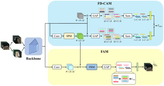
Figure 2.
C2Net structure. GAP means global average pooling operation. SPM is a strip pooling module. FRM indicates the feature re-association module. Yeffect shows the true effect of the bulls’ attention on the forecast outcomes. LAgg is an aggregation loss function used to guide the feature polymerization process.
2.2. Causal Attention Model Based on Feature Decoupling
The counterfactual attention model, based on causal reasoning [16], guides the learning process of the attention diagram by establishing the causal relationship between the features and predicted results, making the model’s prediction logic more transparent and avoiding the unexplainability of the black box model in deep learning. Since the attention map represents the intensity of attention on different areas of the image, improving local attention learning is vital for accurate classification. In this study, a causal attention model based on feature decoupling (FD-CAM) is proposed. An FD-CAM is a typical counterfactual causal inference framework [17,18] consisting of two branches: a multiple attention branch and a counterfactual attention branch.
Multiple attention branches are used to learn the local attention features of the target. For the input feature map F, CNNs are first used to extract advanced features. Then, context information is collected through a pooling operation for feature aggregation to obtain the multi-head attention mapping , where M is the number of attention channels. Considering the extreme aspect ratio of ship targets, the strip pooling module (SPM) [21] is selected to pool F, as shown in Figure 3. Strip pooling (SP) is a long pool core that can avoid the interference of other spatial dimensions while conducting long-distance feature correlation along one spatial dimension and facilitating the extraction of local features. The SPM can account for global and local features by deploying SP in horizontal and vertical directions and has good adaptability to long ship targets. The feature map obtained by the SPM’s pooling is copied along a specific dimension to restore the shape of W × H × M.

Figure 3.
SPM structure.
To obtain the regional feature set , A and F are multiplied (element by element) and the global average pooling is performed using the formula:
where is the m-th regional feature vector; is the value of the c-th element in the region feature vector ; is the M-th attention map in A and is the c-th feature map in F; GAP is the global average pooling; is the element by element multiplication. The local features of the target are obtained by summing M regional feature vectors, as shown below:
l is essentially a feature weighted by spatial attention, which can be obtained by directly summing the multiple attention forces along the channel direction, multiplying the input features element by element, and implementing the global average pooling. The proof is as follows.
Suppose the sum of multiple attention forces along the channel direction is and the calculation is as follows:
Further derivation leads to the following:
The fully connected layer is selected as the classifier and l is input into to obtain the predicted output of the multiple attention branches:
Counterfactual attention branches are used to explore the influence of multiple attention branches on the final classification results by counterfactual intervention; the input is a randomly generated false attention diagram. The regional feature vector and the local feature vector of the false attention map are calculated in the same way as the multi-head attention using the following formulas:
The prediction results obtained according to the counterfactual local feature vector are:
By calculating the difference between and , we can quantify the impact of the multi-head attention features on the prediction results:
can be understood as the learning objective of the local attention mechanism, that is, the internal correlation between the multiple attention and the predicted results after eliminating the interference of false attention. The cross-entropy loss function is used to guide the learning of association, given by the expression:
where is the truth tag.
The coupling between the features in counterfactual causal reasoning networks is an important factor affecting local attention learning. Inspired by the work of Chen et al. [19], we draw on the feature separation idea of contrast learning, carrying out separation through manual intervention to realize the decoupling of regional features of input images and local features between non-homologous images to obtain more distinctive attention features and prevent the mutual influence of local features in attention learning.
Regional feature decoupling is carried out within each feature set, as shown in Figure 4a. The feature vector in the regional feature set represents the filtering feature of local attention on input feature map F. The essence of the decoupling feature vector is to decouple local attention, which can improve the learning of local classification features by reducing the correlation between the channels of multiple attention maps. In decoupling, combining the vectors in the region feature set is necessary for feature separation. To avoid double computation and ensure computational efficiency, cyclic shift is adopted to sort through the vector set, and decoupling is performed with the vector at the corresponding position in the original set, as shown below:
where is the cyclic shift; s is the shift step size; and are the regional feature set and feature vector obtained by the cyclic shift, respectively; is the decoupling loss of regional features. is the decoupling function, defined as follows:
where and are one-dimensional vectors. Since the input images are transformed in two different ways, the feature aggregation of regional feature vectors between homologous images must be considered. Since two homologous maps correspond to the same target, the attention feature maps of the same channel should have the same focusing region, and the regional feature vectors filtered by them share the same local features. Figure 4b presents the feature aggregation process. The aggregation function is defined as follows:
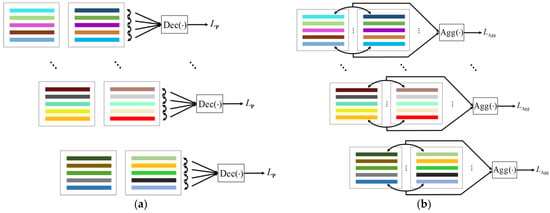
Figure 4.
Schematic diagram of regional feature decoupling and aggregation. (a) Regional feature decoupling; (b) Homology image region feature aggregation.
The loss function used to guide the polymerization process is given by the expression:
where and represent the regional feature vectors of two homologous maps. Algorithm 1 shows the pseudo-code.
| Algorithm 1. Regional feature decoupling and polymerization |
| Input: Homology image region feature set and . The number of attention channels M. Output: Regional feature decoupling loss . Homologous map local feature aggregation loss . Initialization: , . /* The cyclic shift operation is performed on the region feature set R to ensure that the region feature vectors are paired once in the decoupling process. Since the decoupling takes place within the regional feature set, and are no longer represented separately. */ for s in range(M − 1) do /* Cyclic shift s steps. */ /* The vectors are decoupled in pairs. */ for m in range(M) do end end /* Homologous map feature aggregation. */ for m in range(M) do end Return , |
Unlike regional feature decoupling, the local feature decoupling between non-homologous images is de-correlated for instance-level targets. By separating the target from its subclass cluster, we can eliminate the feature adhesion between the targets, avoid feature confusion, and reduce the difficulty of learning causal attention. As shown in Figure 5, the local features of the input image are combined in pairs for the decoupling operation; the decoupling loss is as follows:
where B indicates the input batch size. Note that the local features of the pairwise combination originate from the same input branch and the corresponding input image uses the same transformation operation. Algorithm 2 shows the pseudo-code for the local feature decoupling.
| Algorithm 2. Local feature decoupling of non-homologous images |
| Input: Local features and of the two branches’ input images. The batch size B of the input image. Output: Regional feature decoupling loss Ll. Initialization: Ll = 0. /* Iterate over all local features. */ for i in range(B) do for j in range(B) do # Determine whether it is a local feature of non-homologous image. If it is, perform feature decoupling; otherwise, skip it if i is equal to j then continue else end end end Return Ll |

Figure 5.
Local feature decoupling.
2.3. Feature Aggregation Module
In Section 2.2, based on feature separation in contrast learning, the regional feature representations of homologous maps and the local features of non-homologous maps are separated to decouple the regional features and classes. In this section, the clustering operation in contrast learning is introduced and the feature aggregation module (FAM) is used to pull the FD-CAM-separated features back into the corresponding subclass cluster.
The FAM structure is shown in Figure 2. To input the main stem feature F and multi-head attention diagram, a 1 × 1 convolution is used to reduce the dimension F, and is determined by multiplying the feature map after dimensionality reduction with multiple attention map A pixel by pixel. Each channel focuses on different local areas and are weakly correlated with each other. To realize the re-association between the target’s local features, we designed a feature re-association module (FRM) based on an SP, as shown in Figure 6. Different from the SPM, the FRM strips the pool of the three dimensions of and extends the output dimensions of the three dimensions to obtain the re-association attention diagram , as follows:
where indicates the average pooling of the row dimensions, indicates the average pooling of the column dimensions, and indicates the average pooling of the channel dimensions. indicates a dimension replication operation. , , and are the feature maps of the row dimension, column dimension, and channel dimension after strip pooling.
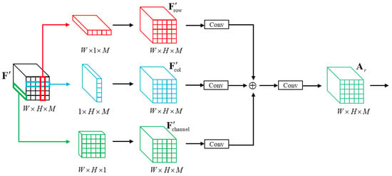
Figure 6.
FRM structure.
The re-association feature map is obtained by using the pair weighting and . Through multi-dimensional information integration, the FRM can consider both the spatial and channel domains to achieve better feature re-association. Global average pooling for is implemented to obtain the feature vector of the target:
To cluster the feature vectors, the clustering centers of various categories must be defined. We adopt the method based on agent loss to realize feature clustering by setting learnable explicit agents for each category and pulling similar feature vectors toward their corresponding proxy vectors. The principle is shown in Figure 7. Considering that a single display agent has certain limitations for fine-grained recognition tasks, this paper follows the method by Chen et al. 2020 [19], setting multiple proxy vectors as the clustering centers for various categories to reduce the clustering difficulty and improve efficiency. Specifically, let the set of proxy vectors be , where n is the number of proxy vectors. The aggregation function is used to pull the feature vector to its proxy vector set:
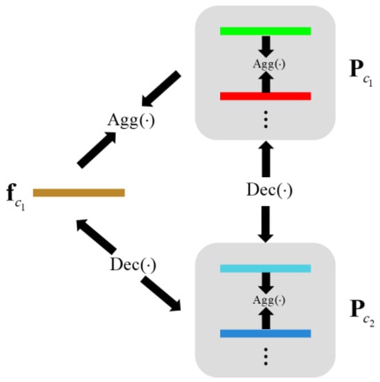
Figure 7.
Principle of feature clustering.
To ensure the separability of the agents between classes and the relevance of the agents within classes, we perform separation operations on the agents of different classes and aggregation operations on the agent vectors of the same class:
where c1 and c2 represent two categories.
Finally, the full-connection layer is used as the classifier to complete the fine-grained classification of ship targets:
where is the predicted result of the category.
2.4. Loss Function
The loss function in this paper mainly includes the loss of the causal attention branch, the loss of the feature aggregation branch, and the loss of classification, which are defined as follows:
is used to guide the feature separation and causal attention learning of the causal attention branches. is used to supervise the feature re-association of the feature aggregation branches and the clustering process of the proxy vectors. uses cross-entropy loss to punish the final classification prediction. The total loss function is defined as:
3. Experiments
This section evaluates the proposed method on a public dataset. First, we introduce the fine-grained classification datasets FGSC-23 [11] and FGSCR-42 [22] used in this paper. Secondly, we elaborate on the specific implementation details used during the experiment, including the environmental version, hardware configuration, training parameters, and dataset processing. We then discuss the ablation experiment design used to assess the performance of each part of the model. Finally, we compare the proposed method with other fine-grained classification methods.
3.1. Datasets
3.1.1. FGSC-23
The FGSC-23 dataset was mainly collected from panchromatic remote sensing images of Google Earth and GF-2 satellites, including about 4080 sliced ship images with a resolution of 0.4–2 m and a size of 40 × 40–800 × 800 pixels. The labeling information of each sample includes a category label, aspect ratio label, and direction label. The classification task is only conducted based on the category label. All samples were divided into training and test sets using a 4:1 ratio. There were 23 categories (Figure 8), 1 non-ship target and 22 ship targets; namely, aircraft carrier (AC), destroyer (DE), landing craft (LC), frigate (FR), amphibious transport dock (ATD), cruiser (CR), Tarawa-class amphibious assault ship (TAA), amphibious assault ship (AS), command ship (CS), submarine (SU), medical ship (MS), combat boat (CB), auxiliary ship (AU), container ship (CT), car carrier (CC), hovercraft (HC), bulk carrier (BC), oil tanker (OT), fishing boat (FB), passenger ship (PS), liquefied gas ship (LG), and barge (BA).
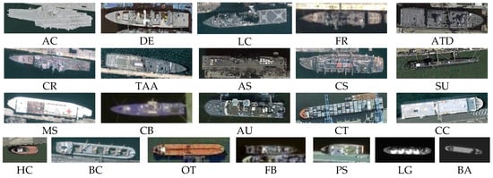
Figure 8.
Samples of the FGSC-23 dataset.
3.1.2. FGSCR-42
The FGSCR-42 dataset comprised 7776 images of common types of ships, ranging from 50 × 50 to 500 × 1500 pixels and obtained from Google Earth and other remote sensing datasets, such as DOTA [23] and HRSC2016 [24]. Under 10 main categories, the ship type consisted of 42 sub-categories; namely, Nimitz class aircraft carrier (NAC), KittyHawk class aircraft carrier (KHCA), Midway class aircraft carrier (MCA), Kuznetsov class aircraft carrier (KNCA), Charles de Gaulle aircraft carrier (CGA), INS Vikramaditya aircraft carrier (IVA), INS Virrat aircraft carrier (IVKA), Ticonderoga class cruiser (TCC), Arleigh Burke class destroyer (ABCD), Akizuki class destroyer (AKCD), Asagiri class destroyer (ASCD), Kidd class destroyer (KDCD), Type 45 destroyer (T45), Wasp class assault ship (WCS), Osumi class landing ship (OCL), Hyuga class helicopter destroyer (HCHD), Lzumo class helicopter destroyer (LCHD), Whitby Island class dock landing ship (WICDL), San Antonio class transport dock (SACTD), Freedom class combat ship (FCC), Independence class combat ship (ICC), Sacramento class support ship (SCS), Crane ship (CS), Abukuma class frigate (ACF), Megayacht (MY), Cargo ship (CGS), Murasame class destroyer (MCD), Container ship (CTS), Towing vessel (TV), Civil yacht (CY), Medical ship (MS), Sand carrier (SC), Tank ship (TS), Garibaldi aircraft carrier (GAC), Zumwalt class destroyer (ZCD), Kongo class destroyer (KGCD), Horizon class destroyer (HCD), Atago class destroyer (ACD), Maestrale class frigate (MCAA), Juan Carlos I Strategic Projection Ship (JCSPS), Mistral class amphibious assault ship (MCF), and San Giorgio class transport dock (SGTD). A sample example is shown in Figure 9. We trained and tested the model by dividing the dataset into training and test sets in a 1:1 ratio.
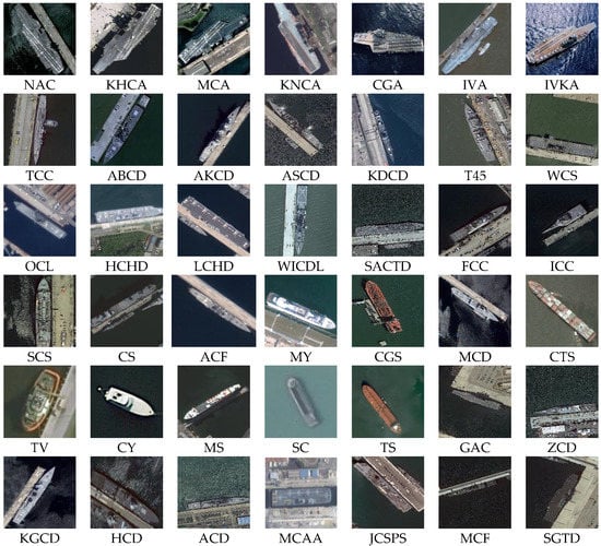
Figure 9.
Samples of the FGSCR-42 dataset.
3.2. Evaluation Metrics
Overall accuracy (OA) and average accuracy (AA) were selected as the main metrics for the model’s performance. Assessing the forecast accuracy from an overall perspective, OA determines the proportion of correctly predicted samples from the total samples without classifying them and is given by the expression:
where TP, TN, FP, and FN are the number of true positive samples, true negative samples, false positive samples, and false negative samples, respectively. The higher the OA value, the higher the prediction accuracy and the better the model’s effect.
In comparison, AA focuses on the prediction of each category and evaluates the model’s performance by calculating the average recall rate of all categories using the following:
where C is the number of categories and is the recall of class c, which is used to represent the recognition accuracy of the class. The prediction results were then visualized through confusion matrix (CM) and 2D feature distribution to provide a more intuitive assessment of the model’s performance.
3.3. Implementation Details
The experiments were conducted using the Windows 10 operating system and the development platform was Anaconda Pytorch 1.6.0 + CUDA10.1. All experiments were performed on a laptop equipped with an Inter(R) Core(TM) i7-10875H @ 2.30GHz CPU and a NVIDIA GeForce RTX 2080 Super with Max-Q Design (8G of video memory) GPU. We used the stochastic gradient descent (SGD) [25] as the optimizer and adjusted the learning rate using the cosine annealing algorithm [26]. The model trained 200 epochs on the FGSC-23 dataset with a batch size of 16,100 epochs on the FGSCR-42 dataset and 10 epochs in the warm-up training. The backbone network was the ResNet50 [27], pre-trained on ImageNet [28]. The initial learning rate and weight decay were set to 0.001 and the momentum to 0.9. The proxy vector was initialized with Xavier Uniform [29]. To ensure that the input image was not distorted, we used the edge-filling method to scale all the image sizes to 224 × 224 pixels and carried out image enhancement operations by random horizontal flip, random vertical flip, and random rotation, among others.
3.4. Ablation Studies
We then designed a series of ablation experiments to study the effects of various parts of C2Net on classification accuracy, including the FD-CAM and FAM branches. The FD-CAM analysis focused on the causal attention structure and feature decoupling, while the FAM analysis focused on the FRM and feature aggregation. The experiment was conducted on the FGSC-23 datasets and FGSCR-42 datasets; the results are shown in Table 1 and Table 2. In addition, we also explored the influence of some hyperparameters and functional forms on the model’s performance.

Table 1.
The ablation experiments of the different parts of the C2Net on the FGSC-23 dataset.

Table 2.
The ablation experiments of the different parts of C2Net on the FGSCR-42 dataset.
3.4.1. Effectiveness of the FD-CAM
The FD-CAM was used to determine the local attention diagram of channel decoupling. We conducted ablation experiments on the counterfactual causal attention structure and the feature decoupling operation in the FD-CAM using the control variable method to study the influence of each part on the classification performance. As shown in Table 1 and Table 2, compared with the backbone network, the OA and AA, using only the counterfactual causal attention structure, increased by 1.95% and 1.81%; the OA and AA, using only the feature decoupling operation, increased by 1.83% and 1.71%, respectively. The complete FD-CAM achieved 90.90% OA and 90.63% AA on the FGSC-23 and 94.19% AA on the FGSCR-42. The results in Table 2 show that when the FAM-only classifier was used as the baseline model, the AA of the FD-CAM increased by 1.20%. The experimental results indicate that the counterfactual causal attention structure improved the learning quality of local attention by changing the model’s discriminant mode, while feature decoupling eliminated feature redundancy by separating the local features; thus, improving the classification performance. In addition, the classification accuracy of the combined FD-CAM and FAM was higher compared to using only the FAM, confirming the effectiveness and feasibility of the FD-CAM.
To assess the model’s effect more directly, we visualized the confusion matrix and two-dimensional feature distribution diagrams of the stochastic neighbor embedding (t-SNE) algorithm [30], as shown in Figure 10 and Figure 11. The horizontal axis of the confusion matrix shows the prediction results, the vertical axis presents the actual results, and the diagonal refers to the accuracy of each class. From Figure 10, the confusion matrix with the most chaotic color distribution occurred when only the trunk network was used. When the FD-CAM was used, the color distribution became more concentrated in the diagonal line, and the recall rate for most kinds improved. Comparing the feature distributions in Figure 11, the FD-CAM had a higher aggregation degree than the trunk network, and C2Net had a higher aggregation degree than only the FAM. The results suggest that the local feature decoupling of the FD-CAM can reduce the mutual interference between the discriminant features of different target parts, providing high-quality local features and effectively improving classification performance.
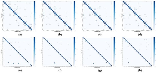
Figure 10.
Confusion matrix. (a–d) Confusion matrices of the main trunk network, backbone network +FD-CAM, backbone network +FAM, and C2Net on the FGSC-23 test set, respectively; (e–h) are the confusion matrices of the FGSCR-42 test set.
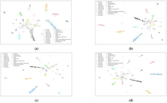
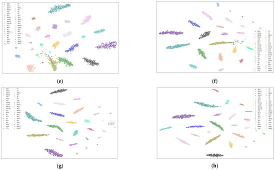
Figure 11.
2D feature distribution. (a–d) Feature distributions of the main trunk network, backbone network +FD-CAM, backbone network +FAM, and C2Net on the FGSC-23 test set, respectively; (e–h) feature distributions of the FGSCR-42 test set.
3.4.2. Effectiveness of the FAM
Ablation experiments were conducted on two FAM parts: the FRM and characteristic polymerization. In Table 1, when the baseline model was the primary trunk network, the FRM increased in OA from 88.83% to 91.02% and in AA from 88.66% to 90.60%. The experimental results in Table 2 also show that the classification accuracy of the FRM improved after the addition. When the baseline model was only the FD-CAM, the FRM increased in AA from 94.19% to 95.01%, indicating that multi-dimensional information integration can more comprehensively establish the correlation between features.
After the FRM completes the feature association, the clustering of target features is implemented through the feature aggregation operation. Without the use of the FD-CAM, the improvement in classification accuracy by feature aggregation is limited. When combined with the FD-CAM, the feature aggregation reclusters locally decoupled features, improving the OA and AA by 2–3%. The FAM and FD-CAM, mainly composed of the FRM and feature aggregation, realize the asynchronous feature learning process together. When the FD-CAM was used alone, the OA decreased by 2.18% and the AA decreased by 0.5–1.5% compared with C2Net. As shown in Figure 11, the FAM can effectively pull the features of similar targets to the corresponding clustering center, resulting in a relatively compact feature distribution.
3.4.3. Effectiveness of Attention Channels
Multi-head attention mapping improves the model’s fine-grained recognition ability by learning the detailed local features of different parts of the ship target. To explore the influence of attention density on the model’s classification ability, ablation experiments were conducted on different channel numbers; the results are shown in Table 3. When the number of channels was 16, the OA reached 92.48% and the AA reached 91.43%. When the number of channels is too small, the model cannot learn enough detailed features. Conversely, if the number of channels is too large, there will be feature redundancy among the channels, resulting in considerable feature ambiguity during decoupling and affecting the learning of the model’s local attention.

Table 3.
The performance of attention channels M on the FGSC-23 dataset.
3.4.4. Effectiveness of the Proxy Vector Number
As the attribute agent in the target category, the display agent plays the clustering center in the feature aggregation stage. In this paper, multiple proxy vectors are set for each category as a clustering center group, which enlarges the range of the clustering center and reduces the dependence on a single central point. This can improve the effect and efficiency of clustering to a certain extent. In order to find the optimal number of agent vectors, the OA and AA of different proxy vector numbers were compared; the results are presented in Table 4. The best classification accuracy was achieved when n = 2, with an OA of 92.48% and an AA of 91.43%. The effectiveness of the clustering center group can be verified by comparing it with the experimental results of a single agent. However, when the number of agents is too large, the central cluster becomes loose, which is not conducive to feature aggregation. In addition, using large numbers of agents would increase the training burden, resulting in the inadequate learning of the agent vector and adversely impacting feature aggregation.

Table 4.
The performance of proxy vector number n on the FGSC-23 dataset.
3.4.5. Effectiveness of the Decoupling Function and Aggregation Function
Is this what you mean: Both the decoupling and aggregation functions are compound logarithmic and cosine distance functions. Logarithmic loss is a common loss function in logistic regression tasks; its domain is a finite interval (0,1). The value range for the cosine distance is also a finite interval (−1,1), so the vector regression problem can be transformed into a binary classification problem. The advantages of logarithmic function in probability distribution characterization can be used to improve feature decoupling and aggregation. To evaluate the effectiveness of the logarithmic form, a set of ablation experiments were employed to compare the influence of the two proposed compound functions and the ordinary cosine distance on the experimental results. As shown in the results in Table 5, both and helped to improve the model’s classification. When used separately, increased the OA by 0.85% and the AA by 1.61%, while increased the OA by 0.25% and the AA by 0.94%. When used together, the OA increased by 1.95% and the AA increased by 1.72%, confirming the method’s effectiveness.

Table 5.
The performance of and on the FGSC-23 dataset.
3.5. Comparisons with Other Methods
The proposed C2Net was then compared with other methods to analyze the model’s fine-grained classification performance. The experiments were first conducted on the FGSC-23 dataset, calculating the recognition accuracy, OA, and AA of 23 sub-categories; the results are shown in Table 6.

Table 6.
Accuracy (%) of the different methods on the testing set of the FGSC-23 dataset. The overall accuracy (OA), average accuracy (AA), and the accuracy of each category are listed.
Inception v3 [32], DenseNet121 [33], MobileNet [35], and Xception [37] are general CNNs and classification is carried out by extracting high-level features from images; their main limitation is that only global features are available, while detailed features are ignored. To address the problem of limited samples, FDN [5], DCL [31], and B-CNN [34] improve the recognition accuracy of remote sensing targets through multi-feature fusion and pseudo-tag training; however, they do not consider the fusion of different receptive field features, resulting in a low utilization rate of local information. ME-CNN [6] combines the CNN, Gabor filter, LBP operator, and other means, in extracting multiple features, providing more information than the FDN. T2FTS [38] solves the long-tail recognition problem in remote sensing images using a hierarchical distillation framework. FBNet [39] uses a feature-balancing strategy to strengthen the representation of weak details and refine local features through an iterative interaction mechanism, addressing the problem of fuzzy or missing target details. PMG [36] and LGFFE [40] have been proposed for fine-grained classification tasks under weak supervision, providing more discriminant features through multi-level feature learning.
In contrast, the proposed C2Net method takes into account the adhesion redundancy among the local features, improves feature quality by asynchronous feature learning, and fully utilizes the detailed local features of targets. The experimental results show that C2Net achieved the highest accuracy, with an OA of 92.48% and an AA of 91.43%, 3.03–10.18% and 3.36–9.89% higher than the other approaches. Because we do not expand the dataset to balance the number of categories, class 11 has the smallest number in the dataset and the recognition accuracy is lower than other methods, at 65.00%. To verify the generalization of the proposed method, we conducted further tests using the FGSCR-42 dataset. As shown in Table 7, C2Net achieved the highest AA of 95.42%, higher by 2.21~5.50% compared with other methods, proving the model’s strength in the fine-grained classification of ship targets.

Table 7.
SOTA comparison on the FGSCR-42 dataset.
4. Conclusions
This study explored the fine-grained classification of ship objects in optical remote-sensing images and developed a comparative learning network based on causal attention. In this network, the FD-CAM and FAM are used to decouple and aggregate features in an asynchronous manner to improve the quality of local features. The FD-CAM is designed based on the counterfactual causal attention model to eliminate false associations between the results and features by strengthening the predictive logic of the model. To prevent feature adhesion, the FD-CAM uses a decoupling function to separate features and obtain a high-quality local attention weight. The partial attention weight is used as the input of the FAM to weigh the trunk, and the FRM is used to achieve feature re-association. Then, the feature clustering process is guided by proxy loss to achieve a fine-grained classification. Experimental results on two common ship datasets showed that the proposed method achieved optimal accuracy and better classification performance than other methods. Its limitation is that the number of model parameters is not lightweight enough and there is a certain gap between the practical engineering application. In future work, we plan to study the decoupling and aggregation of local features further, to improve the fine-grained classification accuracy, and on this basis, explore a lighter weight classification model.
Author Contributions
Conceptualization, C.P.; methodology, C.P.; validation, C.P.; formal analysis, C.P. and R.L.; investigation, C.P. and Q.H.; writing, original draft preparation, C.P.; writing, review and editing, R.L. and Q.H.; visualization, C.P., C.N. and W.L. (Wei Liu); supervision, R.L. and W.L. (Wanjie Lu) All authors have read and agreed to the published version of the manuscript.
Funding
This research was funded by the National Youth Science Foundation under Grant No. 41901378.
Conflicts of Interest
The authors declare no conflict of interest.
References
- Wang, N.; Li, B.; Wei, X.; Wang, Y.; Yan, H. Ship detection in spaceborne infrared image based on lightweight CNN and multisource feature cascade decision. IEEE Trans. Geosci. Remote Sens. 2020, 59, 4324–4339. [Google Scholar] [CrossRef]
- You, Y.; Ran, B.; Meng, G.; Li, Z.; Liu, F.; Li, Z. OPD-Net: Prow detection based on feature enhancement and improved regression model in optical remote sensing imagery. IEEE Trans. Geosci. Remote Sens. 2020, 59, 6121–6137. [Google Scholar] [CrossRef]
- Liu, Z.; Yuan, L.; Weng, L.; Yang, Y. A high resolution optical satellite image dataset for ship recognition and some new baselines. In Proceedings of the International Conference on Pattern Recognition Applications and Methods, Porto, Portugal, 24–26 February 2017; SciTePress: Vienna, Austria, 2017; Volume 2, pp. 324–331. [Google Scholar]
- Oliveau, Q.; Sahbi, H. Learning attribute representations for remote sensing ship category classification. IEEE J. Sel. Top. Appl. Earth Obs. Remote Sens. 2017, 10, 2830–2840. [Google Scholar] [CrossRef]
- Shi, Q.; Li, W.; Tao, R. 2D-DFrFT based deep network for ship classification in remote sensing imagery. In Proceedings of the 2018 10th IAPR Workshop on Pattern Recognition in Remote Sensing (PRRS), Beijing, China, 19–20 August 2018; IEEE: New York, NY, USA, 2018; pp. 1–5. [Google Scholar]
- Shi, Q.; Li, W.; Tao, R.; Sun, X.; Gao, L. Ship classification based on multifeature ensemble with convolutional neural network. Remote Sens. 2019, 11, 419. [Google Scholar] [CrossRef]
- Shi, J.; Jiang, Z.; Zhang, H. Few-shot ship classification in optical remote sensing images using nearest neighbor prototype representation. IEEE J. Sel. Top. Appl. Earth Obs. Remote Sens. 2021, 14, 3581–3590. [Google Scholar] [CrossRef]
- Xiao, Q.; Liu, B.; Li, Z.; Ni, W.; Yang, Z.; Li, L. Progressive data augmentation method for remote sensing ship image classification based on imaging simulation system and neural style transfer. IEEE J. Sel. Top. Appl. Earth Obs. Remote Sens. 2021, 14, 9176–9186. [Google Scholar] [CrossRef]
- Goring, C.; Rodner, E.; Freytag, A.; Denzler, J. Nonparametric part transfer for fine-grained recognition. In Proceedings of the IEEE Conference on Computer Vision and Pattern Recognition, Columbus, OH, USA, 23–28 June 2014; pp. 2489–2496. [Google Scholar]
- Branson, S.; Van Horn, G.; Belongie, S.; Perona, P. Bird species categorization using pose normalized deep convolutional nets. arXiv 2014, preprint. arXiv:1406.2952. [Google Scholar]
- Zhang, X.; Lv, Y.; Yao, L.; Xiong, W.; Fu, C. A new benchmark and an attribute-guided multi-level feature representation network for fine-grained ship classification in optical remote sensing images. IEEE J. Sel. Top. Appl. Earth Obs. Remote Sens. 2020, 13, 1271–1285. [Google Scholar] [CrossRef]
- Chen, Y.; Zhang, Z.; Chen, Z.; Zhang, Y.; Wang, J. Fine-Grained Classification of Optical Remote Sensing Ship Images Based on Deep Convolution Neural Network. Remote Sens. 2022, 14, 4566. [Google Scholar]
- Lin, T.Y.; Maji, S. Improved bilinear pooling with cnns. arXiv 2017, preprint. arXiv:1707.06772. [Google Scholar]
- Huang, L.; Wang, F.; Zhang, Y.; Xu, Q. Fine-Grained Ship Classification by Combining CNN and Swin Transformer. Remote Sens. 2022, 14, 3087. [Google Scholar] [CrossRef]
- Meng, H.; Tian, Y.; Ling, Y.; Li, T. Fine-grained ship recognition for complex background based on global to local and progressive learning. IEEE Geosci. Remote Sens. Lett. 2022, 19, 1–5. [Google Scholar] [CrossRef]
- Pearl, J.; Mackenzie, D. The Book of Why: The New Science of Cause and Effect; Basic Books: New York, NY, USA, 2018. [Google Scholar]
- Rao, Y.; Chen, G.; Lu, J.; Zhou, J. Counterfactual attention learning for fine-grained visual categorization and re-identification. In Proceedings of the IEEE/CVF International Conference on Computer Vision, Nashville, TN, USA, 20–25 June 2021; pp. 1025–1034. [Google Scholar]
- Xiong, W.; Xiong, Z.; Cui, Y. An Explainable Attention Network for Fine-Grained Ship Classification Using Remote-Sensing Images. IEEE Trans. Geosci. Remote Sens. 2022, 60, 1–14. [Google Scholar] [CrossRef]
- Chen, J.; Chen, K.; Chen, H.; Li, W.; Zou, Z.; Shi, Z. Contrastive Learning for Fine-Grained Ship Classification in Remote Sensing Images. IEEE Trans. Geosci. Remote Sens. 2022, 60, 1–16. [Google Scholar] [CrossRef]
- Zhan, X.; Xie, J.; Liu, Z.; Ong, Y.S.; Loy, C.C. Online deep clustering for unsupervised representation learning. In Proceedings of the IEEE/CVF Conference on Computer Vision and Pattern Recognition, Seattle, WA, USA, 13–19 June 2020; pp. 6688–6697. [Google Scholar]
- Hou, Q.; Zhang, L.; Cheng M, M.; Feng, J. Strip pooling: Rethinking spatial pooling for scene parsing. In Proceedings of the IEEE/CVF Conference on Computer Vision and Pattern Recognition, Seattle, WA, USA, 13–19 June 2020; pp. 4003–4012. [Google Scholar]
- Di, Y.; Jiang, Z.; Zhang, H. A public dataset for fine-grained ship classification in optical remote sensing images. Remote Sens. 2021, 13, 747. [Google Scholar] [CrossRef]
- Xia, G.S.; Bai, X.; Ding, J.; Zhu, Z.; Belongie, S.; Luo, J.; Zhang, L. DOTA: A large-scale dataset for object detection in aerial images. In Proceedings of the IEEE Conference on Computer Vision and Pattern Recognition, Salt Lake City, UT, USA, 18–23 June 2018; pp. 3974–3983. [Google Scholar]
- Liu, Z.; Wang, H.; Weng, L.; Yang, Y. Ship rotated bounding box space for ship extraction from high-resolution optical satellite images with complex backgrounds. IEEE Geosci. Remote Sens. Lett. 2016, 13, 1074–1078. [Google Scholar] [CrossRef]
- Bordes, A.; Bottou, L.; Gallinari, P. SGD-QN: Careful Quasi-Newton Stochastic Gradient Descent. J. Mach. Learn. Res. 2009, 10, 1737–1754. [Google Scholar]
- Loshchilov, I.; Hutter, F. Sgdr: Stochastic gradient descent with warm restarts. arXiv 2016, preprint. arXiv:1608.03983. [Google Scholar]
- Xie, S.; Girshick, R.; Dollár, P.; Tu, Z.; He, K. Aggregated residual transformations for deep neural networks. In Proceedings of the IEEE Conference on Computer Vision and Pattern Recognition, Honolulu, HI, USA, 21–26 July 2017; pp. 1492–1500. [Google Scholar]
- Deng, J.; Dong, W.; Socher, R.; Li, L.J.; Li, K.; Fei-Fei, L. Imagenet: A large-scale hierarchical image database. In Proceedings of the 2009 IEEE Conference on Computer Vision and Pattern Recognition, Miami, FL, USA, 20–25 June 2009; IEEE: New York, NY, USA, 2009; pp. 248–255. [Google Scholar]
- Glorot, X.; Bengio, Y. Understanding the difficulty of training deep feedforward neural networks. J. Mach. Learn. Res. 2010, 9, 249–256. [Google Scholar]
- Van der Maaten, L.; Hinton, G. Visualizing data using t-SNE. J. Mach. Learn. Res. 2008, 9, 2579–2605. [Google Scholar]
- Zhao, W.; Tong, T.; Wang, H.; Zhao, F.; He, Y.; Lu, H. Diversity Consistency Learning for Remote-Sensing Object Recognition with Limited Labels. IEEE Trans. Geosci. Remote Sens. 2022, 60, 1–10. [Google Scholar] [CrossRef]
- Szegedy, C.; Vanhoucke, V.; Ioffe, S.; Shlens, J.; Wojna, Z. Rethinking the inception architecture for computer vision. In Proceedings of the IEEE Conference on Computer Vision and Pattern Recognition, Las Vegas, NV, USA, 27–30 June 2016; pp. 2818–2826. [Google Scholar]
- Huang, G.; Liu, Z.; Van Der Maaten, L.; Weinberger, K.Q. Densely connected convolutional networks. In Proceedings of the IEEE Conference on Computer Vision and Pattern Recognition, Honolulu, HI, USA, 21–26 July 2017; pp. 4700–4708. [Google Scholar]
- Lin, T.Y.; RoyChowdhury, A.; Maji, S. Bilinear CNN models for fine-grained visual recognition. In Proceedings of the IEEE International Conference on Computer Vision, Santiago, Chile, 7–13 December 2015; pp. 1449–1457. [Google Scholar]
- Howard, A.G.; Zhu, M.; Chen, B.; Kalenichenko, D.; Wang, W.; Weyand, T.; Adam, H. Mobilenets: Efficient convolutional neural networks for mobile vision applications. arXiv 2017, preprint. arXiv:1704.04861. [Google Scholar]
- Du, R.; Chang, D.; Bhunia, A.K.; Xie, J.; Ma, Z.; Song, Y.-Z.; Guo, J. Fine-grained visual classification via progressive multi-granularity training of jigsaw patches. In Proceedings of the Computer Vision—ECCV 2020: 16th European Conference, Glasgow, UK, 23–28 August 2020; Springer International Publishing: Cham, Switzerland, 2020; pp. 153–168. [Google Scholar]
- Chollet, F. Xception: Deep learning with depthwise separable convolutions. In Proceedings of the IEEE Conference on Computer Vision and Pattern Recognition, Honolulu, HI, USA, 21–26 July 2017; pp. 1251–1258. [Google Scholar]
- Zhao, W.; Liu, J.; Liu, Y.; Zhao, F.; He, Y.; Lu, H. Teaching teachers first and then student: Hierarchical distillation to improve long-tailed object recognition in aerial images. IEEE Trans. Geosci. Remote Sens. 2022, 60, 1–12. [Google Scholar] [CrossRef]
- Zhao, W.; Tong, T.; Yao, L.; Liu, Y.; Xu, C.; He, Y.; Lu, H. Feature balance for fine-grained object classification in aerial images. IEEE Trans. Geosci. Remote Sens. 2022, 60, 1–13. [Google Scholar] [CrossRef]
- Lv, Y.; Zhang, X.; Xiong, W.; Cui, Y.; Cai, M. An end-to-end local-global-fusion feature extraction network for remote sensing image scene classification. Remote Sens. 2019, 11, 3006. [Google Scholar] [CrossRef]
- Nauta, M.; Van Bree, R.; Seifert, C. Neural prototype trees for interpretable fine-grained image recognition. In Proceedings of the IEEE/CVF Conference on Computer Vision and Pattern Recognition, Nashville, TN, USA, 19–25 June 2021; pp. 14933–14943. [Google Scholar]
- Chen, Y.; Bai, Y.; Zhang, W.; Mei, T. Destruction and construction learning for fine-grained image recognition. In Proceedings of the IEEE/CVF Conference on Computer Vision and Pattern Recognition, Long Beach, CA, USA, 16–20 June 2019; pp. 5157–5166. [Google Scholar]
- Yu, C.; Zhao, X.; Zheng, Q.; Zhang, P.; You, X. Hierarchical bilinear pooling for fine-grained visual recognition. In Proceedings of the European Conference on Computer Vision (ECCV), Munich, Germany, 8–14 September 2018; pp. 574–589. [Google Scholar]
- Zhuang, P.; Wang, Y.; Qiao, Y. Learning attentive pairwise interaction for fine-grained classification. Proc. AAAI Conf. Artif. Intell. 2020, 34, 13130–13137. [Google Scholar] [CrossRef]
- Zheng, H.; Fu, J.; Zha, Z.J.; Luo, J. Looking for the devil in the details: Learning trilinear attention sampling network for fine-grained image recognition. In Proceedings of the IEEE/CVF Conference on Computer Vision and Pattern Recognition, Long Beach, CA, USA, 16–20 June 2019; pp. 5012–5021. [Google Scholar]
- Wang, Y.; Lv, K.; Huang, R.; Song, S.; Yang, L.; Huang, G. Glance and focus: A dynamic approach to reducing spatial redundancy in image classification. Adv. Neural Inf. Process. Syst. 2020, 33, 2432–2444. [Google Scholar]
Disclaimer/Publisher’s Note: The statements, opinions and data contained in all publications are solely those of the individual author(s) and contributor(s) and not of MDPI and/or the editor(s). MDPI and/or the editor(s) disclaim responsibility for any injury to people or property resulting from any ideas, methods, instructions or products referred to in the content. |
© 2023 by the authors. Licensee MDPI, Basel, Switzerland. This article is an open access article distributed under the terms and conditions of the Creative Commons Attribution (CC BY) license (https://creativecommons.org/licenses/by/4.0/).