Abstract
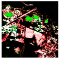
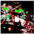
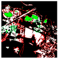
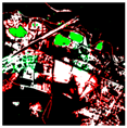
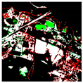
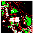
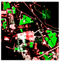
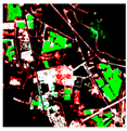
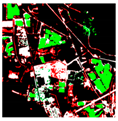
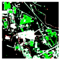
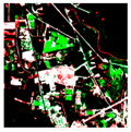
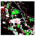
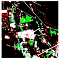
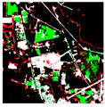
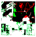
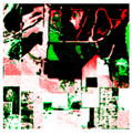
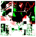
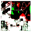
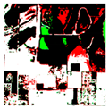
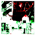
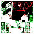
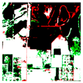
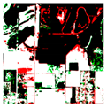
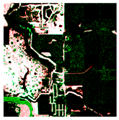
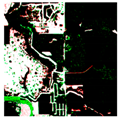
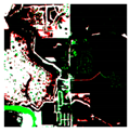
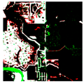
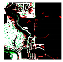
Advances in deep learning and computer vision are making significant contributions to flood mapping, particularly when integrated with remotely sensed data. Although existing supervised methods, especially deep convolutional neural networks, have proved to be effective, they require intensive manual labeling of flooded pixels to train a multi-layer deep neural network that learns abstract semantic features of the input data. This research introduces a novel weakly supervised approach for pixel-wise flood mapping by leveraging multi-temporal remote sensing imagery and image processing techniques (e.g., Normalized Difference Water Index and edge detection) to create weakly labeled data. Using these weakly labeled data, a bi-temporal U-Net model is then proposed and trained for flood detection without the need for time-consuming and labor-intensive human annotations. Using floods from Hurricanes Florence and Harvey as case studies, we evaluated the performance of the proposed bi-temporal U-Net model and baseline models, such as decision tree, random forest, gradient boost, and adaptive boosting classifiers. To assess the effectiveness of our approach, we conducted a comprehensive assessment that (1) covered multiple test sites with varying degrees of urbanization, and (2) utilized both bi-temporal (i.e., pre- and post-flood) and uni-temporal (i.e., only post-flood) input. The experimental results showed that the proposed framework of weakly labeled data generation and the bi-temporal U-Net could produce near real-time urban flood maps with consistently high precision, recall, f1 score, IoU score, and overall accuracy compared with baseline machine learning algorithms.
1. Introduction
The effects of global climate change are expected to lead to increases in the intensity of extreme precipitation and flood events across all climate regions, ranging from arid to humid regions [1]. Accurate and timely flood inundation maps are essential sources of information for various stakeholders, including government agencies, contractors of the U.S. Federal Emergency Management Agency (FEMA), lenders, insurance agents, land developers, realtors, community planners, property owners, and others who need to plan for and mitigate damage caused by floods. These maps provide vital information on the extent and severity of flood events, which can assist in developing effective response plans and mitigation strategies. By having access to current and accurate information on flood inundation, these stakeholders can take proactive measures to protect lives, property, and infrastructure, reducing the overall impact of flood events on communities and the economy [2]. While these stakeholders seek different types of quantitative and qualitative information, their primary aim is the acquisition of near-real-time flood extent maps showing inundated areas, especially in densely populated urban areas. In this context, remote sensing (RS) technologies, such as optical imaging and synthetic aperture radar (SAR), have been used for flood extent mapping. Recent advances and improvements in satellite sensors, data accessibility, applications, and services have made remotely sensed data more accessible and efficient for disaster management [3]. Particularly, the development of novel tools for flood mapping such as machine learning and computer vision technologies applied to multispectral (MS) images is rapidly evolving [4].
Flood mapping through RS can be performed through various image processing techniques and machine learning (ML) models, such as Support Vector Machines (SVMs [5]), decision trees [6], random forests [7], hidden Markov trees [8], and logistic regression (LR) [9], which can classify or extract flooded areas. These traditional ML models perform well for RS applications; however, the model generalizability is limited due to a small number of training data used. Alternatively, with an increasing large volume of multi-temporal MS RS data being freely accessible for emergency response, deep learning (DL), a sub-field of ML, has significantly boosted the performance of flood mapping. Compared with traditional ML algorithms requiring handcrafted image features for classification and regression, DL is unique in its automatic data-driven representation learning capability [10]. In particular, deep convolutional neural networks (CNNs) [11], such as fully convolutional nets (FCNS) [11] and U-Net [12], often achieve higher classification accuracy than the traditional methods for flood detection using RS datasets [13].
While modern data-driven machine learning approaches (especially deep neural networks) have proved to be powerful for image classification, the main bottleneck is the lack of ground truth labels for model training and testing. In particular, CNN-based models require large volumes of training images with corresponding high-quality labels, whereas labeling pixel-wise ground truth flood mask is a laborious and time-consuming task. Although many efforts have been made to learn image representations in an un-/self-supervised manner without hand labeling [14,15,16,17], quite a few hand labels are still required to train a classifier with learned representations, hindering the applications in emergency disaster response. Since the time-consuming hand labeling is infeasible in operational disaster response workflows, automatic label generation is the key to a real-time flood mapping system. In addition, although researchers have extensively studied machine and deep learning models for flood mapping, they have largely focused on rural areas with a relatively homogeneous image background [18,19,20]. Challenges that come with mapping flooded urban and vegetated areas include shadowing caused by manmade infrastructure, undesired spatial resolution, and cloud cover. For instance, if the spatial resolution is not high enough, the mixture of spectral properties of flood water and other land components in pixels makes it difficult to visually identify flooded pixels from dense buildings and trees by human annotators, resulting in inaccurate labels for model training and testing. Furthermore, there is a lack of focus on incorporating both pre- and post-flood images for pixel-wise flood mapping that can classify each pixel as flooded or non-flooded [7,18,20]. As such, there is an urgency in improving flood extent mapping in urban areas to address the challenges rising from heterogeneous land cover and a lack of flood extent ground truth labels.
The primary challenge addressed in this study is the automatic generation of training labels for a supervised machine learning model that achieves fast and accurate classification results, eliminating the need for time-consuming human annotations. Particularly, this study proposes a novel, weakly supervised pixel-wise flood mapping framework, which uses multi-temporal MS imagery to classify flooded and non-flooded pixels in urban areas. This approach eliminates the need for human-labeled datasets during model training. In an effort to foster the reproducibility and reusability of this study, we have made the model code and a subset of the project’s data publicly accessible on the Internet. The code and data can be found at the following repository: https://github.com/vongkusolkit/bitemporalUNet, accessed on 29 May 2023.
To sum up, the contributions of this work are elaborated as follows:
- (1)
- The proposed framework for producing weakly labeled data allows for model training without relying on human-annotated labels. This framework enables supervised models to be trained using weak labels that can be automatically generated in near realtime (less than 2 min), showcasing its potential for deployment in operational workflows to assist emergency disaster response.
- (2)
- This paper develops a bi-temporal U-Net model that enhances the quality of feature extraction by utilizing both pre- and post-flood images for flood mapping. By implementing a traditionally uni-temporal deep learning model to accept a bi-temporal input, the proposed model paves the way for potential model implementations to accommodate multi-temporal input. The proposed bi-temporal model with the weak-label generation framework demonstrates a robust approach for near-real-time flood mapping across study sites within cities with different degrees of urbanization, demonstrating its capability for transferability (i.e., generalizability) in emergency response for future flooding events.
- (3)
- The experiments conducted in this study validated the effectiveness of flood mapping across different types of input as well as baseline models used for flood detection.
2. Model Background and Considerations
RS has emerged as a powerful tool for mapping inundation due to its capacity for temporal and spatial coverage. Flood mapping using RS data mostly employs two main strategies: pixel-wise and patch-wise mapping. In patch-wise flood mapping, an image patch containing multiple pixels is classified, and these patches are created from dividing the entire study area imagery into non-overlapping patches [17]. Meanwhile, pixel-wise flood mapping methods classify each pixel into a category (e.g., flooded or non-flooded), typically applying either manual feature extraction methods or machine learning models. This section introduces relevant works on pix-wise flood mapping.
2.1. Manual Feature Extraction
MS or optical satellite imagery is widely used for pixel-wise flood mapping as the flood can be analyzed in a more straightforward way with simpler pre-processing due to the abundant spectral information associated with floodwater. When the presence of clouds and their shadow in MS imagery hides informative pixels, radar data are used instead for mapping flood inundation areas. Otherwise, MS imagery is a robust method for generating flood inundation maps. This study will only utilize MS imagery and not radar data for comparing different methods of flood inundation mapping.
Several rapid flood mapping techniques rely on spectral indices derived from spectral data and apply threshold values to the ratios for identifying areas (or pixels) corresponding to water [21,22,23,24]. McFeeters et al. [25] proposed the Normalized Difference Water Index (NDWI) using near-infrared (NIR) and green channels of Landsat that can delineate and enhance open water features. By taking advantage of the NIR and green spectral bands, the NDWI can enhance water bodies in a satellite image. The NDWI is calculated as , where and represent the green and near-infrared surface reflectance bands, respectively.
However, the NDWI can also lead to an overestimation of water bodies since it is sensitive to building structures. To remove built-up land noise, the Modified NDWI (MNDWI) is proposed by substituting the NIR band with the middle-infrared (MIR) band. Specifically, the MNDWI is calculated as , where represents a middle-infrared band such as TM band 5. The MNDWI can efficiently suppress the signal from built-up land, which would be useful for flood inundation mapping in urban areas [26]. Both the NDWI and the MNDWI can be computed from the satellite data with values ranging from −1 to +1, and pixels with values greater than 0 are labeled as water [25,26]. Alternatively, Ouma and Tateishi [22] introduced a water index (WI) to quantify shoreline changes using Landsat Thematic Mapper (TM) and Enhanced Thematic Mapper (ETM+) data. The WI is based on a logical combination of the Tasseled Cap Wetness (TCW) index and the NDWI. Feyisa et al. [27] introduced the Automated Water Extraction Index (AWEI) improving classification accuracy in areas that include shadow and dark surfaces that other classification methods (e.g., MNDWI) often fail to classify correctly.
2.2. Image Segmentation
In recent years, image processing and machine learning have emerged as prominent tools for mapping floods using RS imagery. In the realm of flood management, image processing involves a range of methods and technologies, including edge detection, object detection, and image segmentation. Specifically, image segmentation is a crucial approach within image processing for pixel-wise classification, leveraging the concepts of similarity and discontinuity to analyze remotely sensed images obtained from either optical or radar satellites.
2.2.1. Discontinuity Detection through Edge Detection
Edge detection techniques analyze the intensity variations between pixels and their surrounding neighborhoods to identify significant changes (i.e., discontinuities) in an image. When a substantial intensity difference occurs, indicating a clear transition, an edge is detected. Due to the segmentation capability of the edge detection algorithm, different objects within an image can be separated or classified by detecting discontinuities in pixel grayscale values [28]. Edge detection techniques have proven useful in identifying features such as roads, buildings, and houses within images [29]. Among the various edge detection operators, the Canny and Sobel edge detectors [28,30] are widely utilized algorithms for object detection. The Sobel operator computes the gradient magnitude of an image using a 3 × 3 convolution mask that augments differences in gray values (i.e., takes the absolute value of the rate of change in light intensity in the direction that maximizes the value for each pixel), highlighting the edges in the image. Billa et al. [30] used the Sobel filter to detect water lines from SAR images. The Canny detection method enhances the Sobel edge operator by eliminating irrelevant noisy edges from the output of the Sobel and thinning the edges to a width of one pixel. Zhang et al. [28] employed and evaluated Canny edge detection to identify floods in real time by analyzing river water levels.
2.2.2. Similarity Detection through Histogram Thresholding and K-Means Clustering
Histogram thresholding and k-means clustering are widely used techniques for similarity detection in image segmentation due to their straightforward computation process [31,32]. Various thresholding algorithms have been proposed to optimally segment an image into two classes (e.g., flooded and non-flooded), including Otsu’s method, mean, and bimodal histogram thresholding. Histogram thresholding methods presume the presence of two classes of pixels, foreground and background, with the threshold value being the optimal value that distinguishes these two classes. Otsu’s method calculates the optimal value by maximizing the variance between the two classes (inter-class variance) to minimize the intra-class variance. Mean thresholding simply takes the mean of the image as the optimal value. Last, bimodal thresholding smooths the image histogram until it exhibits only two peaks and takes the local minimum as the optimal value.
Rather than using a histogram, k-means clustering calculates the centroids of a specified number of clusters (k) and takes each point to the cluster with the nearest centroid from the respective data point, typically defined through Euclidean distance. The process is iterative with the centroids of each cluster recalculated after each grouping to minimize the sum of distances between data points and their cluster centroids across all clusters. One advantage of k-means clustering over histogram thresholding is its ability to consider more than two classes in an image. Additionally, k-means clustering is less susceptible to noise as it is not influenced by the image histogram. However, the value of k needs to be defined during algorithm initialization, and determining the optimal value for k can be challenging in multiclass scenarios. In this study, binary classification is employed for flooded and non-flooded pixels, thus setting k to 2.
2.3. Machine/Deep Learning Models
While the aforementioned classical RS techniques (e.g., histogram thresholding) can yield satisfactory results for identifying inundated areas [33], pixel-based classification and the use of AI have been the preference to map floods and perform assessments of large-scale disaster areas. Notably, advances in deep learning and computer vision have made significant contributions to disaster mitigation when combined with RS data. Machine learning techniques, such as random forests (RF) and SVM, are typically used in RS land use and land cover classifications due to their superiority over classical RS techniques [34]. Deep learning approaches for semantic segmentation to detect features, such as clouds and cloud shadows, have far outperformed traditional methods that solely rely on RS and image processing techniques by leveraging learning-based methods with training data that can automatically learn informative features and make decisions, including making predictions to map flood extents or to assess the flood damage [20].
2.3.1. Supervised Learning Algorithm
With the increasing availability of high-resolution spatial and spectral data that capture complex details of land features, more information can be extracted for flood maps with higher accuracy. Consequently, more sophisticated machine learning methods are required to extract flood information from these images. One widely adopted approach in this category is SVM [35]. Other traditional machine learning algorithms include decision tree classifiers [6], random forests [7], hidden Markov trees [8], and LR [9].
In addition to traditional machine learning algorithms, deep learning models are also widely used to map floods due to their adaptability and generalization capabilities. In the context of fully supervised segmentation, many excellent models have emerged based on CNN. A popular architecture is the FCN, where the encoder down-samples the input image to a smaller size (while gaining more channels) through a series of convolutions, and the decoder up-samples the encoded output using either bilinear interpolation or a sequence of transpose convolutions [36]. Despite its effectiveness, the FCN architecture suffers from checkerboard artifacts caused by uneven overlap during the process of decoding. Another challenge is the poor resolution at boundaries due to information loss during the encoding process. To mitigate these challenges, the U-Net architecture implements skip connections (from the output of convolution blocks to the corresponding input of the transposed convolution block at the same level) on the FCN. This allows for better gradient flow and enables information from multiple scales of the image size to be utilized [12]. Information from higher resolutions aids in classification, while information from lower resolutions helps with segmentation and localization. Accordingly, Li and Demir [37] extracted water bodies from Sentinel-1 satellite imagery based on the U-Net model. Similarly, this study employed the traditional U-Net architecture, with enhancements made through a bi-temporal design that combined both pre- and post-flood images as input and concatenated them before decoding to improve flood mapping performance.
2.3.2. Weakly Supervised Learning Algorithm
The weakly supervised learning algorithm covers several processes aimed at building predictive models by learning from weak supervision. The three common types of weak supervision include incomplete supervision, inexact supervision, and inaccurate supervision. Incomplete supervision occurs when only a subset of training data is labeled. Inexact supervision refers to situations where the training data are labeled, but the labels may not precisely represent the desired ground truth. Last, inaccurate supervision arises when there are some inaccurate or low-quality labels in the training data. Zhao et al. [38] applied the weakly labeled support vector machine (WELLSVM) to assess flood susceptibility in the metropolitan areas, and the WELLSVM outperformed traditional supervised machine learning models including LR, artificial neural network (ANN), and SVM. In addition, Bonafilia et al. [39] evaluated the performances of FCNN models trained from different subsets of Sentinel-1 imagery, including automatically generated and human-annotated ground truth labels. Their research findings revealed that FCNN models trained on abundant automatically generated labels from optical RS algorithms outperformed models trained on limited manually labeled data. Thus, this study explored the weakly supervised learning algorithm, using inexact supervision. The model was trained on a substantial number of automatically generated labels from MS imagery captured during major flood events in urban areas.
In summary, while existing supervised methods have demonstrated effectiveness, they require intensive human labeling of flooded pixels to train multi-layer deep neural networks that capture abstract semantic features from the input data [10]. Furthermore, training a deep neural network solely on a single human-annotated ground truth flood mask limits its transferability to different flood scenarios due to the highly variable image background for different flooded events. Consequently, such supervised models cannot perform in real time for upcoming disasters. To this end, this research proposes a weakly supervised pixel-wise flood mapping framework that can automatically classify flooded and non-flooded pixels in urban areas using bi-temporal MS imagery, eliminating the need for human-labeled datasets in model training.
3. Materials and Methods
3.1. Case Study
For this study, we selected two urban sites that were affected by flooding events, namely, the 2018 Hurricane Florence flood in Lumberton, North Carolina, and the 2017 Hurricane Harvey flood in Houston, Texas. These study sites were characterized by dense residential, industrial, and commercial areas, which were severely flooded. The dataset was taken from the PlanetScope satellite where the images were surface reflectance products with four spectral bands (B, G, R, and NIR) and a spatial resolution of 3 m ground sample distance (GSD).
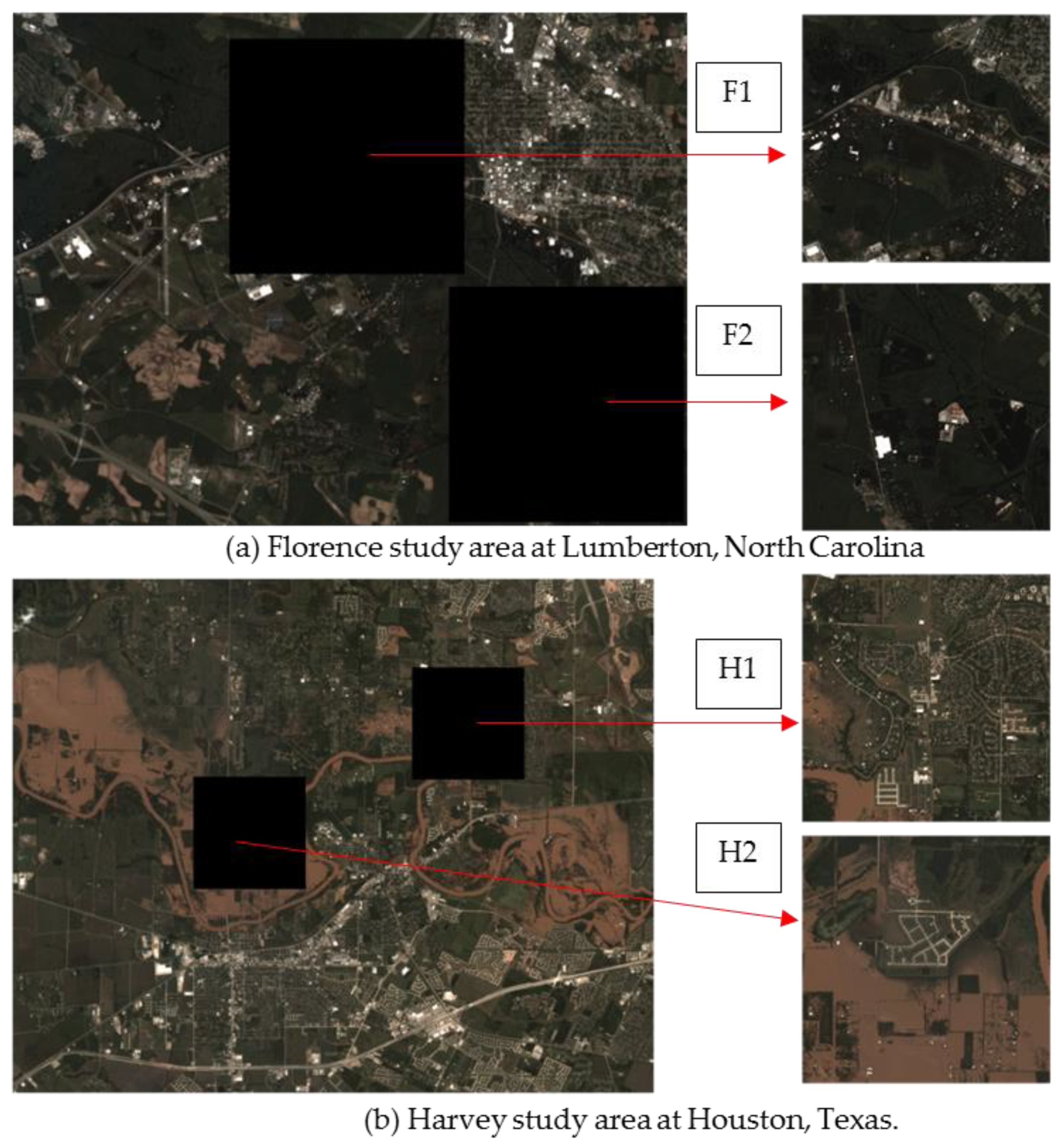
We obtained pre- and post-flood event Planet MS images of Florence on 30 August 2018 and 18 September 2018, respectively. These images had a size of 2240 × 2940 pixels. Two image subsets from the Florence flood, sites F1 and F2 (1024 × 1024 pixels each), were set aside for testing and validation, whereas the rest of the Florence image was used for training (Figure 1a). The next step involved preprocessing the images for model training and testing. To do this, we cropped each image into 336 non-overlapping tiles with each tile including 140 × 140 pixels; 238 tiles (~70%) were used for training, 49 were used for validating (~15%), and 49 were used for testing (~15%).

Figure 1.
Florence (a) and Harvey (b) study areas where F1, F2, H1, and H2 are test sites, while the rest of the images are used for training.
Similarly, we used the pre- (31 July 2017) and post- (31 August 2017) Planet MS images of the Harvey flood event. The full extent of the Harvey flood event was of size 4705 × 5860 pixels. Two image subsets, H1 and H2, of size 1024 × 1024 pixels each, were taken from the Harvey pre- and post-flood images and were used for testing and validation, leaving the rest of the scenes for training (Figure 1b). After cropping the images into 1451 non-overlapping tiles with each tile including 140 × 140 pixels, 1353 tiles (~93%) were used for training, 49 were used for validating (~3.5%), and 49 were used for testing (~3.5%).
3.2. Methodology
3.2.1. Weakly Labeled Flood Map Generation for Model Training
The proposed framework sought to enhance the performance of existing pixel-wise flood mapping methods without the need for labor-intensive manual labeling. Particularly, we capitalized on change detection on bi-temporal data (e.g., pre- and post-event) and the distinct spectral signatures of water and applied a weakly supervised model to generate a weakly labeled flood map in near-real time, requiring less than 2 min to complete (for our image size). The weakly labeled generation framework was developed based on the evaluations conducted during the Florence case study, as ground truth data for the full-sized image were only available for Florence and not for the Harvey case study. Therefore, the accuracy of the full-sized weakly labeled flood map could only be assessed for the Florence flood. Next, the best-case approach for generating the Florence weakly labeled flood map was applied to the Harvey flood.
Problem Formulation
Given a pair of pre- and post-flood MS images , we cropped them into rows by columns of non-overlapping tile pairs , where and represent the tile coordinates. Each tile had dimensions of 140 × 140 pixels and consisted of four bands. This study proposed a weakly supervised framework Ƒ for generating the flood map , which can be represented as
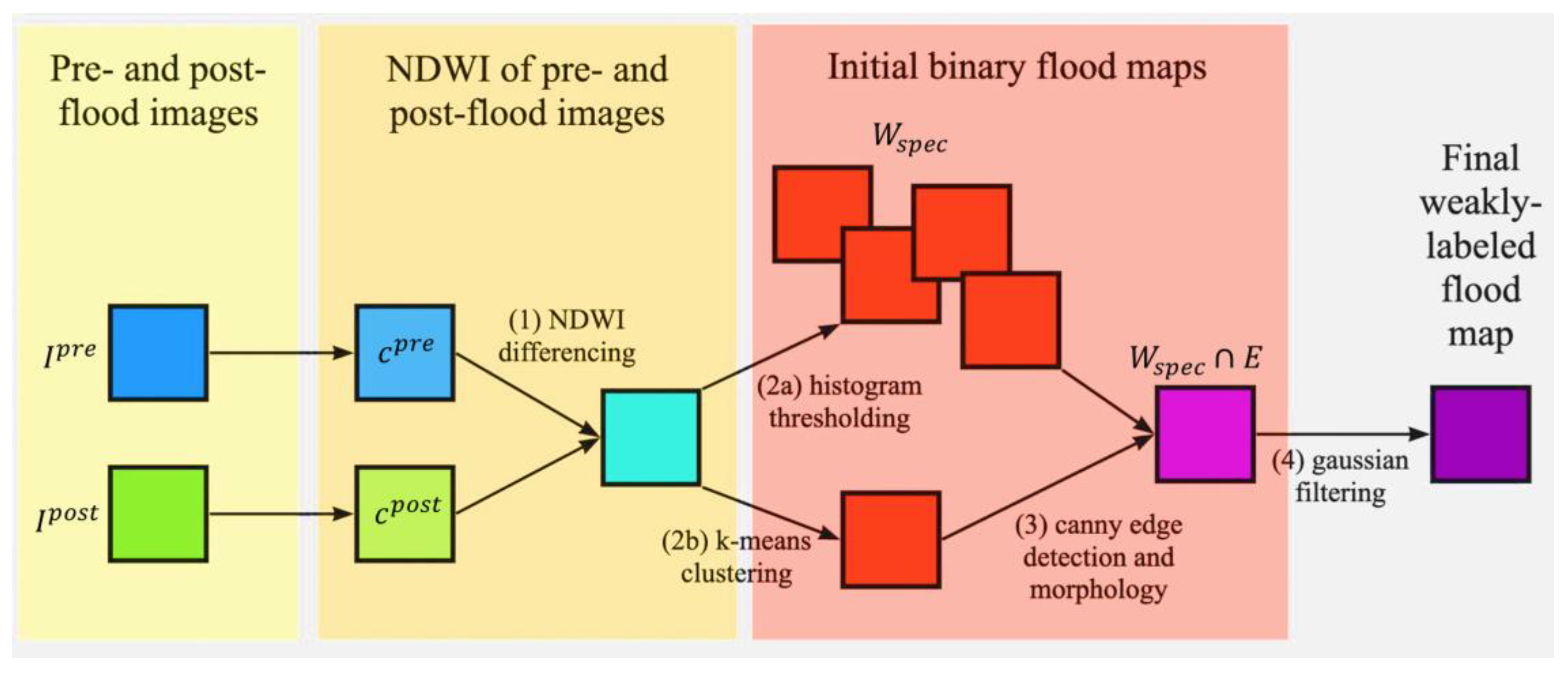
where refer to the three interlocking modules within the framework Ƒ, including (1) change detection for initial feature extraction for weakly labeling; (2) spectral and spatial filtering to eliminate non-flooded changes; and (3) bi-temporal UNet architecture for final feature extraction and flood mapping. The steps followed by the proposed flood mapping scheme are illustrated in Figure 2.
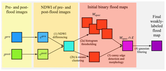
Figure 2.
Workflow of the proposed framework for generating a weakly labeled flood map for model training.
Change Detection
Given the pre- and post-flood images were captured less than a month apart, we assumed that the land cover changes over the study areas were flood-related only. To extract initial features, the NDWI values were computed from the pre- and post-flood images. For each pre- and post-flood image tile , the difference between the NDWI values was obtained as .
Spectral and Spatial Filtering
Since noise and other errors could cause false alarms in the initial change map , spectral and spatial filtering were designed to improve the accuracy of weak labels for subsequent model training by leveraging the spectral signatures and spatial topology of floodwaters (Figure 2). First, spectral filtering was applied to to remove noise from changes unrelated to flooding (e.g., shadows, built structures, or radiometric or geometric errors), through histogram thresholding and k-means clustering. This resulted in an initial binary flood map , where flooded pixels were assigned a label of1 and non-flooded pixels were labeled as 0. Five initial flood maps were generated using two methods: histogram thresholding and k-means clustering. Four of the five flood maps were obtained through histogram thresholding by different methods: mean thresholding , bimodal-minimum thresholding , Otsu’s method , and thresholding at 1.25 standard deviation (std) from the mean (threshold value: 0.159; mean: 0.055; standard deviation: 0.083). The fifth flood map was derived through k-means clustering .
Next, to minimize false positives present in all generated flood maps, Canny edge detection and morphological operations were then applied to remove the background noise (Figure 3). Spatial filtering through Canny edge detection was performed on , which exhibited the highest precision (0.672) and lowest number of false positives among the five initial flood maps. The resulting edge image further passed through Dilation, a morphological operation, to generate .
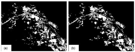
Figure 3.
Comparison of Florence initial flood map before (a) and after (b) noise removal through Canny edge detection.
To eliminate false positives in small, isolated areas within the initial flood maps an intersection operation between and was then applied. The resulting intermediate flood map removed spatial noise since the spatial topology of flood movement indicated that flooded pixels tended to be in close proximity to each other. Finally, underwent a Gaussian filter for smoothing, producing a weakly labeled flood map for model training. The final weakly labeled flood map created from provided the highest f1 score (0.573) after background noise removal. Hence, it was selected as the weak labels (i.e., training data) for the model in this study. This process can be summarized through the following equations:
3.2.2. Bi-Temporal UNet Architecture
In the event of a flood, satellite images taken before the event can be leveraged to produce flood maps with improved accuracy in addition to those taken immediately after the event. However, the conventional UNet architecture is designed to accommodate only one input, limiting its potential for change detection analysis. Thus, we modified the UNet architecture enabling the integration of both the pre- and post-flood images . The proposed model architecture is illustrated in Figure 4.
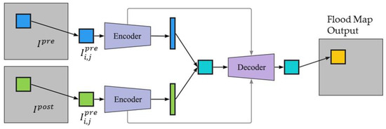
Figure 4.
Architecture of the bi-temporal UNet.
The input pair were passed through a series of convolution and max pooling operations separately during the encoder phase of the model for feature extraction. The encoder, or contraction path, captured the image context by employing a stack of convolutional and max pooling layers. Figure 5 illustrates the encoder and decoder details of the bi-temporal UNet. The convolution operation accepted a 140 × 140 × 4 image stack, where 140 represents the width and the height, and 4 represents the number of spectral bands (R, G, B, and infrared). The max pooling operation reduced the size of the feature map so that there were fewer parameters in the network for subsequent convolutional layers. A 2 × 2 max pool selected the maximum pixel value from every 2 × 2 block in the input feature map, producing a pooled feature map. Both the convolution and pooling operations reduced the size of the image, also known as down-sampling. After a convolution layer and max pooling operation, the filters in the next set of layers were able to see a larger context for the purpose of feature extraction.

Figure 5.
The encoder and decoder architecture details of the bi-temporal UNet.
At the final down-sampling layer, the two outputs were concatenated together and passed through the decoder phase of the model. The decoder, or the symmetric expanding path, enabled precise localization using transposed convolutions. Since the output of semantic segmentation was a high-resolution image (flood mask), where all the pixels were classified, the image needed to be up-sampled from low to high resolution to recover the classified pixel location. Up-sampling was achieved by applying transposed convolution. This operation formed the same connectivity as the normal convolution but in the backward direction. To improve the location precision, skip connections were used at each step of the decoder by concatenating the output of the transposed convolution layers with the corresponding feature maps from the encoder. Thus, the UNet was an end-to-end FCN as it only contained convolutional layers.
In the proposed bi-temporal UNet, data augmentation was performed through random horizontal flips, random up and down flips, and random rotations of 90 degrees. We set the batch size to 12, total number of epochs to 200, and learning rate to 0.01, which reduced by a factor of 0.1 every 10 epochs with no improvement. The optimizer employed was an Adam optimizer with a weight decay of 0.0001. The loss function comprised binary cross entropy () and dice loss (), defined as
where is the target (1 for flooded and 0 for non-flooded), is the probability of class = 1 (flooded), and is the probability of class = 0 (non-flooded) for all pixels in the loss. is the output, and is the target for the loss.
3.2.3. Post-Processing
After obtaining a prediction from the model with a numeric value indicating the likelihood of being flooded for each pixel, we experimented with post-processing using different thresholding methods (mean histogram, bimodal histogram, and Otsu’s method), k-means clustering, and Gaussian smoothing to generate the final binary flood map. The binary flood map with the highest f1 score after post-processing, obtained through thresholding using the mean of the histogram and applying Gaussian smoothing for our case study, was selected as the final flood map.
3.3. Performance Evaluation
Using manually annotated ground truth labels, we computed the number of true positives (TPs), false positives (FPs), true negatives (TNs), and false negatives (FNs) to evaluate the performance of each model using the precision, recall, f1 score, intersection over union (IoU score, also known as Jaccard index), and overall accuracy. The definitions of each evaluation metric are as follows:
where the ground truth label is defined as and model output prediction is defined as for IoU.
In addition to these commonly used evaluation indices for flood mapping, the receiver operating characteristic curve (ROC) and its corresponding area under the curve (AUC) were employed to assess the performance of the model [40]. The ROC curve was constructed by plotting the true positive rate (TP rate) on the Y-axis against the false positive rate (FP rate) on the X-axis. The AUC value, ranging from 0.5 to 1, served as a measure of the model’s performance, with higher values indicating better performance [38,41,42].
4. Results
This section presents the accuracy assessment of the weakly labeled flood map and the experimental results for the bi-temporal UNet, traditional UNet, and baseline models. The baseline models, including DT, RF, Gradient Boosting Classifier (GBC), and AdaBoost, were trained with the proposed weakly labeled flood map and tested with hand-labeled “ground truths”. Table 1 shows the accuracy metrics of the weakly labeled flood map compared with the hand-labeled flood map for the full-sized image, test site F1, and test site F2. The weakly labeled flood map achieved f1 scores of 77%, 87%, and 76% for the full-sized image, site F1, and site F2, respectively.

Table 1.
Evaluation scores of the Florence weakly labeled flood map when evaluated against the hand-labeled flood map in the full-sized image, test site F1, and test site F2.
The evaluation results for the Florence and Harvey floods are displayed in Table 2 and Table 3, respectively. The findings indicated that ensemble methods (e.g., RF, AdaBoost, and GBC), in general, exhibited higher precision but lower recall, resulting in a lower f1 score, IoU, and overall accuracy scores compared with the bi-temporal UNet. The bi-temporal UNet consistently performed well across all evaluation metrics. It is worth noting that the model’s performance improved with the increase in training data size. Consequently, the evaluation scores for the Harvey study areas outperformed those of the Florence study areas.

Table 2.
Model evaluations of weakly labeled Florence flood maps.

Table 3.
Model evaluations of weakly labeled Harvey flood maps.
To evaluate the effectiveness of post-processing methods, results of the bi-temporal UNet model’s prediction before and after applying Gaussian smoothing to different thresholding methods are shown in Table 4 for the Florence flood and Table 5 for the Harvey flood. However, the results showed that using the Gaussian filter for post-processing decreased all evaluation metrics besides recall for both the Harvey and Florence flood sites.

Table 4.
Before and after Gaussian smoothing evaluations of bi-temporal UNet’s Florence flood map prediction on different thresholding/clustering methods.

Table 5.
Before and after Gaussian smoothing evaluations of bi-temporal UNet’s Harvey flood map prediction on different thresholding/clustering methods.
4.1. Flood Event 1: Florence
We tested two areas of the Florence flood: F1 and F2. For each of these areas, we experimented with different input models: post-flood image only and pre- and post-flood images . For the F1 testing area using only post-flood images , the model with the highest f1 score was GBC (0.7695), followed by RF (0.7649), AdaBoost (0.7509), DT (0.7099), and UNet (0.6719). For pre- and post-flood images , the model with the highest f1 score was bi-temporal UNet (0.8928), followed by GBC (0.8410), RF (0.8350), AdaBoost (0.8181), and DT (0.8014). GBC achieved the highest precision (0.8941), but it had a lower recall than the bi-temporal UNet. However, since the precision (0.8877) of bi-temporal UNet was less than 1%, while its recall (0.8980) was more than 10% higher than that of GBC, the bi-temporal UNet achieved the highest f1 (0.8928), IoU (0.8064), and overall accuracy (0.9403) scores.
In the F2 testing area, when using only post-flood images , the model with the highest f1 score was RF (0.6170), followed closely by GBC (0.6166), AdaBoost (0.6097), DT (0.5911), and UNet (0.4734). Using both pre- and post-flood images , the model with the highest f1 score was GBC (0.7834), followed by bi-temporal UNet (0.7800), RF (0.7521), AdaBoost (0.7295), and DT (0.7193). The bi-temporal UNet achieved the highest recall (0.9538) but fell short to the GBC (pre + post), which achieved the highest precision (0.7875), f1 score (0.7834), IoU (0.6440), and overall accuracy (0.8990) scores. This suggested that while the bi-temporal UNet had a high recall, it also generated a considerable number of false positives. A summary of the evaluation metrics for the Florence flood study areas can be found in Table 2.
Once the output prediction map with a numeric value for each pixel was obtained from the model, various thresholding methods were applied to create a final binary flood map. These methods included mean histogram, bimodal histogram, Otsu’s method, and 2-class K-means. For the F1, 2-class k-means clustering produced a binary flood map with the highest f1 score of 0.8928, followed by a tie between the bimodal histogram and Otsu’s method, both scoring 0.8927. The mean histogram method yielded an f1 score of 0.8923. Similarly, for the F2 study area, k-means clustering also produced the highest f1 score of 0.7800, followed by Otsu’s method, bimodal, and mean histogram scores of 0.7715, 0.7482, and 0.7474, respectively. Other evaluation scores for these thresholding methods can be found in Table 4.
4.2. Flood Event 2: Harvey
Similar to the Florence site, we also tested two areas of the Harvey flood: H1 and H2. For the H1 testing area, when using only post-flood images , the model with the highest f1 score was UNet (0.8914), followed by GBC (0.8873), AdaBoost (0.8725), RF (0.8664), and DT (0.8326). When using both pre- and post-flood images , the bi-temporal UNet model outperformed other models with the highest f1 score of 0.9110. It was followed by GBC (0.9017), RF (0.9008), DT (0.8909), and AdaBoost (0.8897). Although AdaBoost achieved the highest precision (0.9299), which was 3% higher than the bi-temporal UNet (0.9015), the bi-temporal UNet had a higher recall (0.9207) by 7% compared with AdaBoost (0.8529). As a result, the bi-temporal UNet achieved the highest recall, f1 score (0.9110), IoU (0.8365), and overall accuracy (0.9131) scores.
For the H2 testing area, when using only post-flood images , the model with the highest f1 score was UNet (0.8771), followed by RF (0.8749), GBC (0.8684), AdaBoost (0.8593), and DT (0.8032). Using both pre- and post-flood images , the bi-temporal UNet achieved the highest f1 score (0.9023), followed by GBC (0.8936), RF (0.8874), AdaBoost (0.8753), and DT (0.8687). Despite GBC (pre + post) having the highest precision (0.9260) and UNet (post-only) having the highest recall (0.9551), the bi-temporal UNet achieved the highest f1 score (0.9023), IoU (0.8220), and overall accuracy (0.9491) scores. The differences in the precision (0.9059) and recall (0.8987) scores compared with GBC and UNet were only 2% and 5.6%, respectively.
A summary of the evaluation metrics for the Harvey study areas can be found in Table 3. Furthermore, Table 5 provides the results of different methods for producing a binary flood map from the model’s output prediction for the Harvey flood. For H1, Otsu’s method yielded the highest f1 score of 0.9110, followed by the mean histogram (0.9109), bimodal histogram (0.9107), and k-means clustering (0.9099). For H2, the mean histogram produced the highest f1 score of 0.9023, followed by Otsu’s method (0.8994), k-means clustering (0.8993), and bimodal histogram (0.8989).
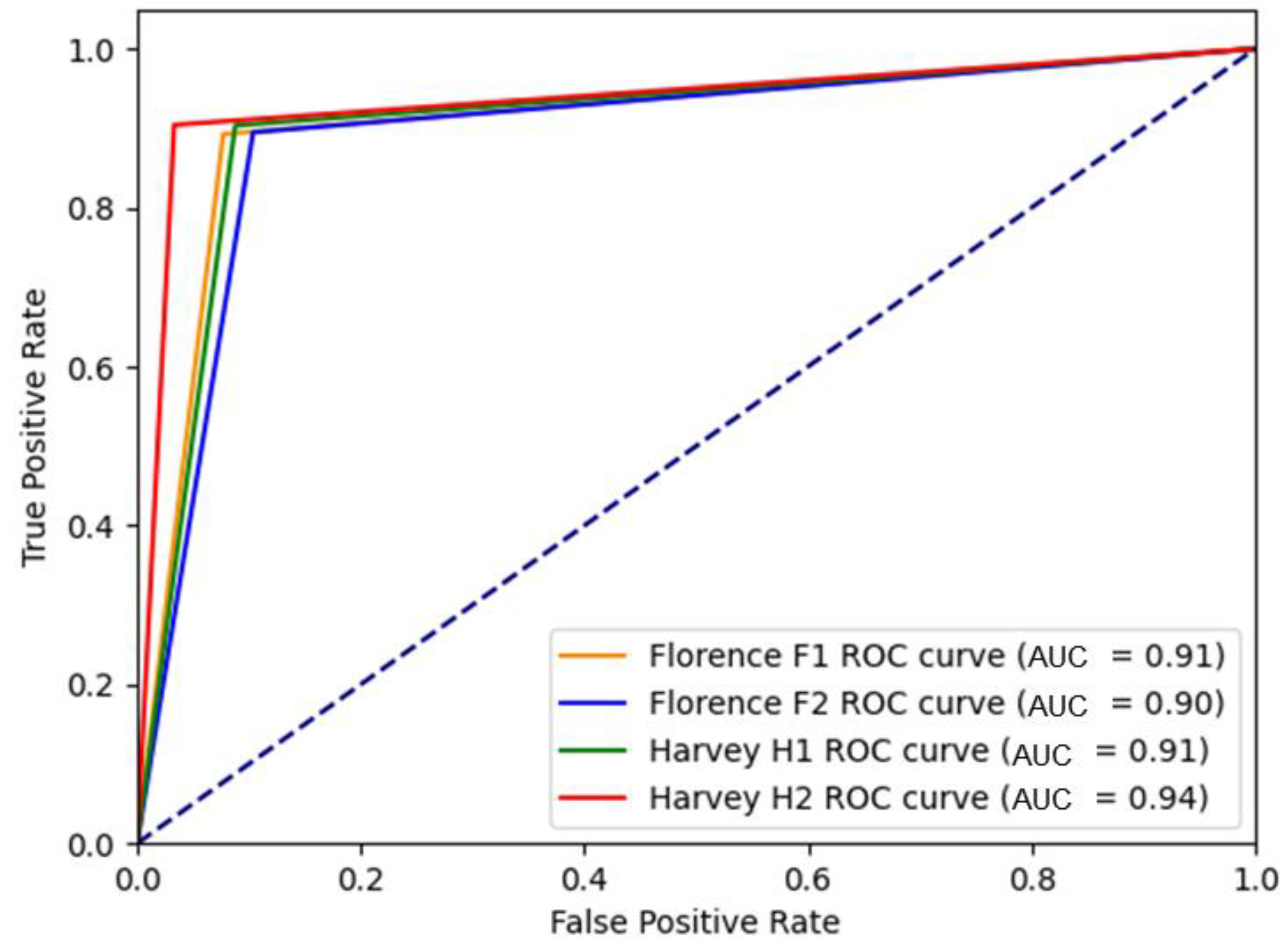
Figure 6 illustrates the ROC curves for the proposed Bi-temporal UNet model across four selected study sites. Notably, the model exhibited strong performance, as indicated by an area under the curve (AUC) equal to or greater than 0.90 for each site. Site H2 attained the highest AUC value of 0.94, followed by sites H1 and F1 with AUC values of 0.91, and finally site F2 with an AUC of 0.90. These findings aligned with the results obtained from other evaluation indices (e.g., OA), with a trend that the Harvey study areas (H1 and H2), benefiting from a larger volume of training data, generally exhibited higher evaluation scores compared with the Florence sites (F1 and F2).
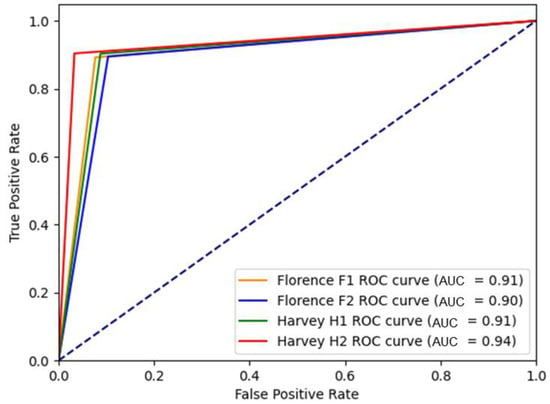
Figure 6.
ROC curve of the proposed bi-temporal model for flood mapping at different test sites.
5. Discussion
Built upon two parallel research subfields including RS and machine learning, this research seeks to improve the performance of current pixel-wise flood mapping approaches without the need for human labels by using bi-temporal RS data and a weakly supervised model. The following sections discuss the implications for model input, classification methods, and the performance of the proposed approach.
5.1. Model Input
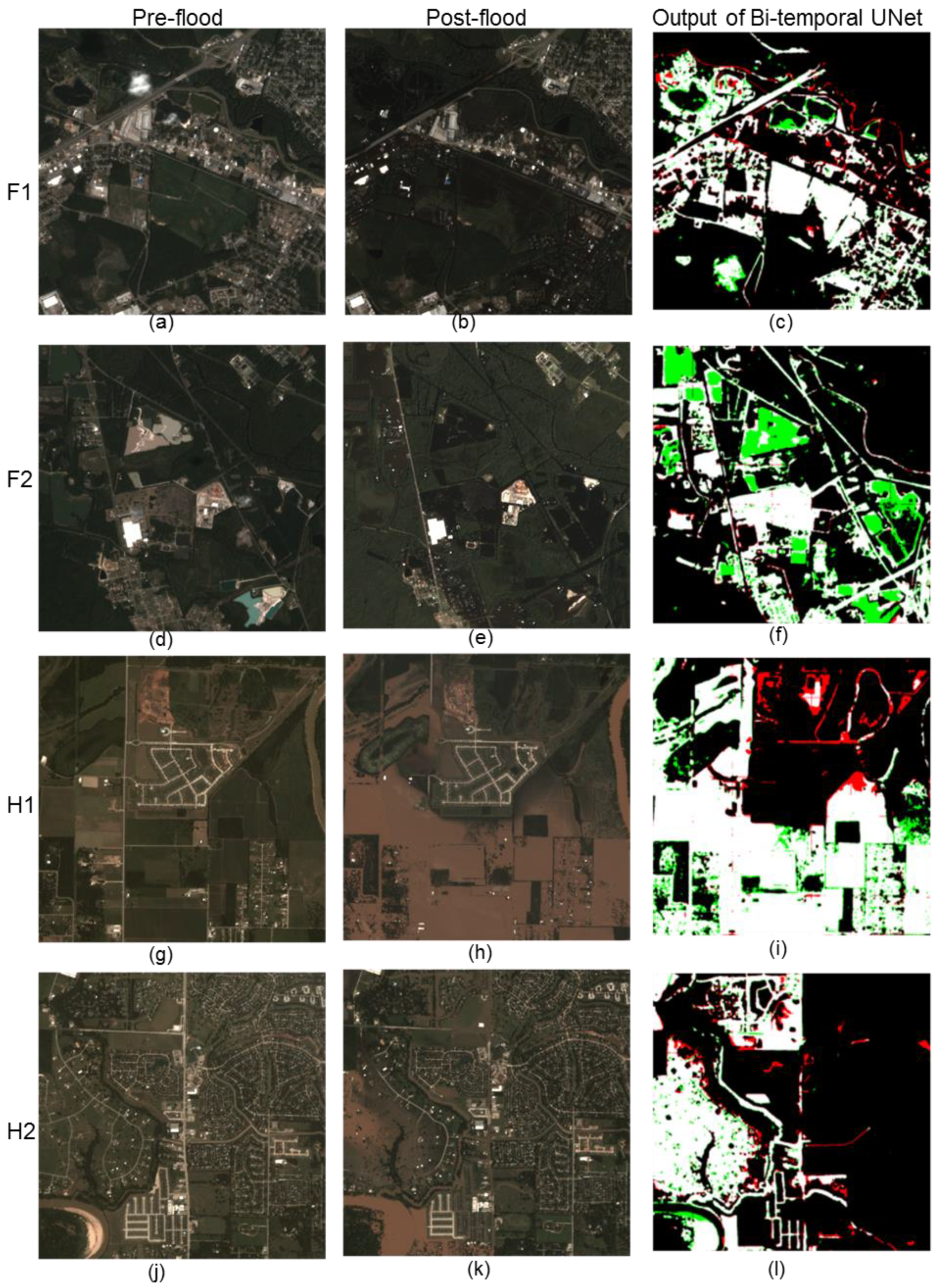
Four different study sites (Florence F1, Florence F2, Harvey H1, and Harvey H2) with different topological objects such as dense buildings, roads, trees, and bare ground were selected to assess the impact of input on model performance (Figure 7). As each inundated object may have different physical and spectral properties, the resulting floodwaters showed inconsistent spectral characteristics where they exhibited various spectra that are mixtures of floodwaters and the neighboring objects (e.g., buildings and trees). This occurrence posed a challenge for pixel-wise classification not only for algorithms but also for human annotators who visually identify floodwaters. Thus, the human-annotated ground truth may be biased to what the annotator defines as a flooded pixel.

Figure 7.
Pre-flood, post-flood, and output of the bi-temporal UNet model, for test sites F1 (a–c), F2 (d–f), H1 (g–i), and H2 (j–l). (Green: false positives; red: false negatives; white: true positives (flood pixels); black: true negatives (non-flood pixels).)
For all test sites except for a specific case in F2, the bi-temporal UNet consistently outperformed the traditional UNet and the other baseline models that also employed both pre- and post-flood images as input. The bi-temporal UNet achieved higher f1 scores by 6.9%, 3.4%, 2.1%, and 1.5% for test sites F1, F2, H2, and H1, respectively. However, in the case of test site F2, the GBC model slightly outperformed the bi-temporal UNet model by 0.3% in terms of the f1 score.
False positive errors were observed primarily at the edges of permanent water bodies, such as ponds and lakes, in test site F1. Conversely, in test site F2, a significant number of false positives occurred within the permanent water bodies themselves. This discrepancy can be attributed to the substantial spectral differences between the open waters in the pre- and post-flood images of F2, unlike F1, where the open waters exhibited similar colors in both images (Figure 7a,b vs. Figure 7d,e). Such scenarios pose a limitation to weakly supervised methods as the algorithm struggles to separate permanent water bodies from floodwaters. Incorporating a method to remove permanent water bodies, either manually or automatically, in the output prediction flood map would significantly increase the accuracy of the prediction.
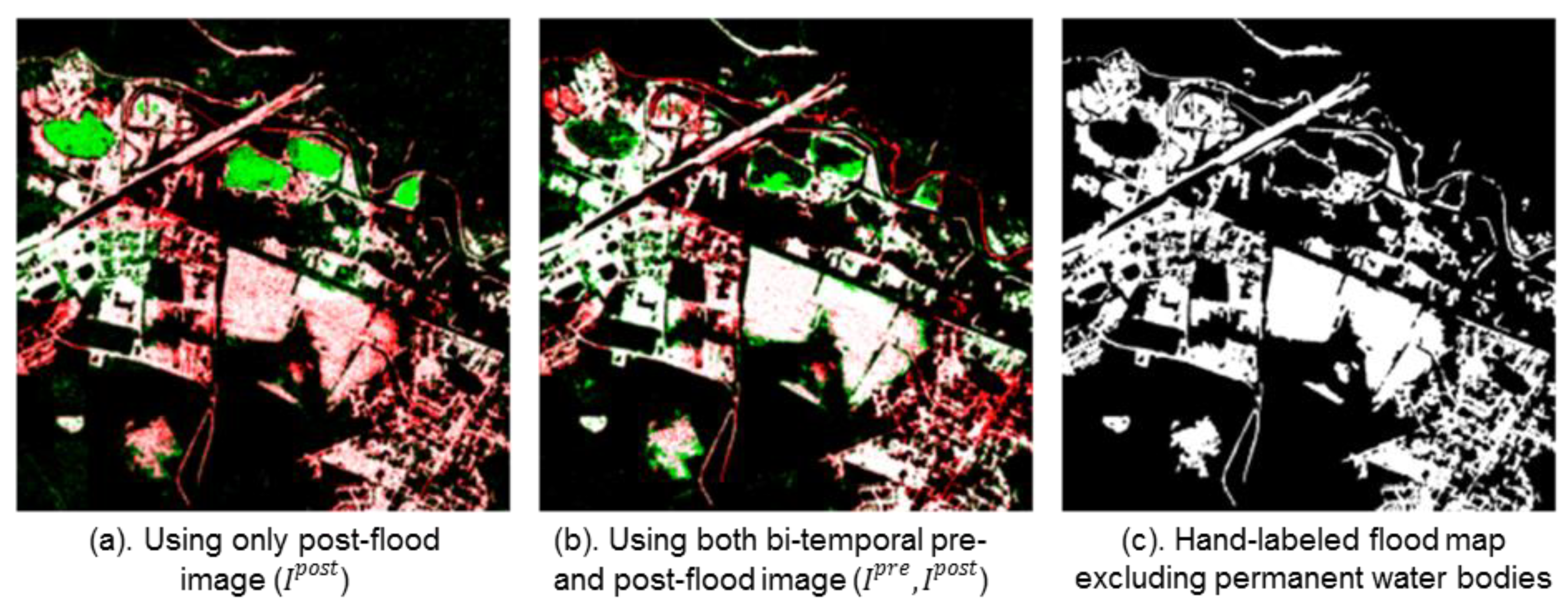
In general, the models exhibited better performance when using bi-temporal flood images as the model input, compared with using only post-flood images . Across all four test sites, there is an improvement of 17.1%, 10.4%, 2.1%, and 1.5% in terms of f1 scores for test sites F2, F1, H2, and H1, respectively. When using only post-flood images as the input, the models failed to distinguish between permanent water bodies (e.g., lakes and rivers) and floodwaters. Consequently, these models tended to classify these permanent water pixels as flooded pixels, leading to an increased number of false positives. However, by incorporating information from the pre-flood image when using bi-temporal images as the model input, the models could effectively differentiate open water with flood water, thereby excluding open water pixels from the prediction. Figure 8 depicts the predictions from the GBC when using only post-flood images and using bi-temporal images as the model input.
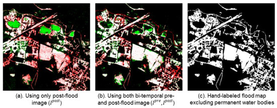
Figure 8.
Study area Florence F1 flood map prediction comparison of different input for GBC (green: false positives; red: false negatives; white: true positives (flood pixels); black: true negatives (non-flood pixels)).
Moreover, models that solely utilized the post-flood image exhibited a higher number of false negatives compared with models using both and , particularly in areas with a higher degree of urbanization. The sites F1 and H2, characterized by a more heterogeneous background image due to urbanization compared with sites F2 and H1, demonstrated this trend. As shown in Table 6, there is a higher number of false negatives, represented in red, for F1 and H2 when using only compared with the models employing both and as the model input. Thus, the integration of additional spectral and temporal information through a bi-temporal input greatly improved the model performance in urbanized areas.

Table 6.
Model predictions for test sites across for Florence and Harvey floods. Green: false positives; red: false negatives; white: true positives (flood pixels); black: true negatives (non-flood pixels).
Although the bi-temporal UNet models outperformed the uni-temporal UNet models by an average of 17.1% and 10.4% for sites F2 and F1 during the Florence flood, it remained inconclusive whether there existed a correlation between the degree of urbanization of the study sites and the type of input. This was further demonstrated by the fact that there was no difference in scores between bi-temporal and uni-temporal models for sites H2 and H1 during the Harvey flood. Despite site H2 being more urbanized than site H1, the average evaluation scores across all models with bi-temporal input were only 2.9% greater than those using only uni-temporal input for both H1 and H2. The limited number of case studies (Harvey and Florence floods) and the lack of consistency in results between the two sites hindered the formation of a conclusive inference.
5.2. Classification Methods for Binarizing Flood Maps
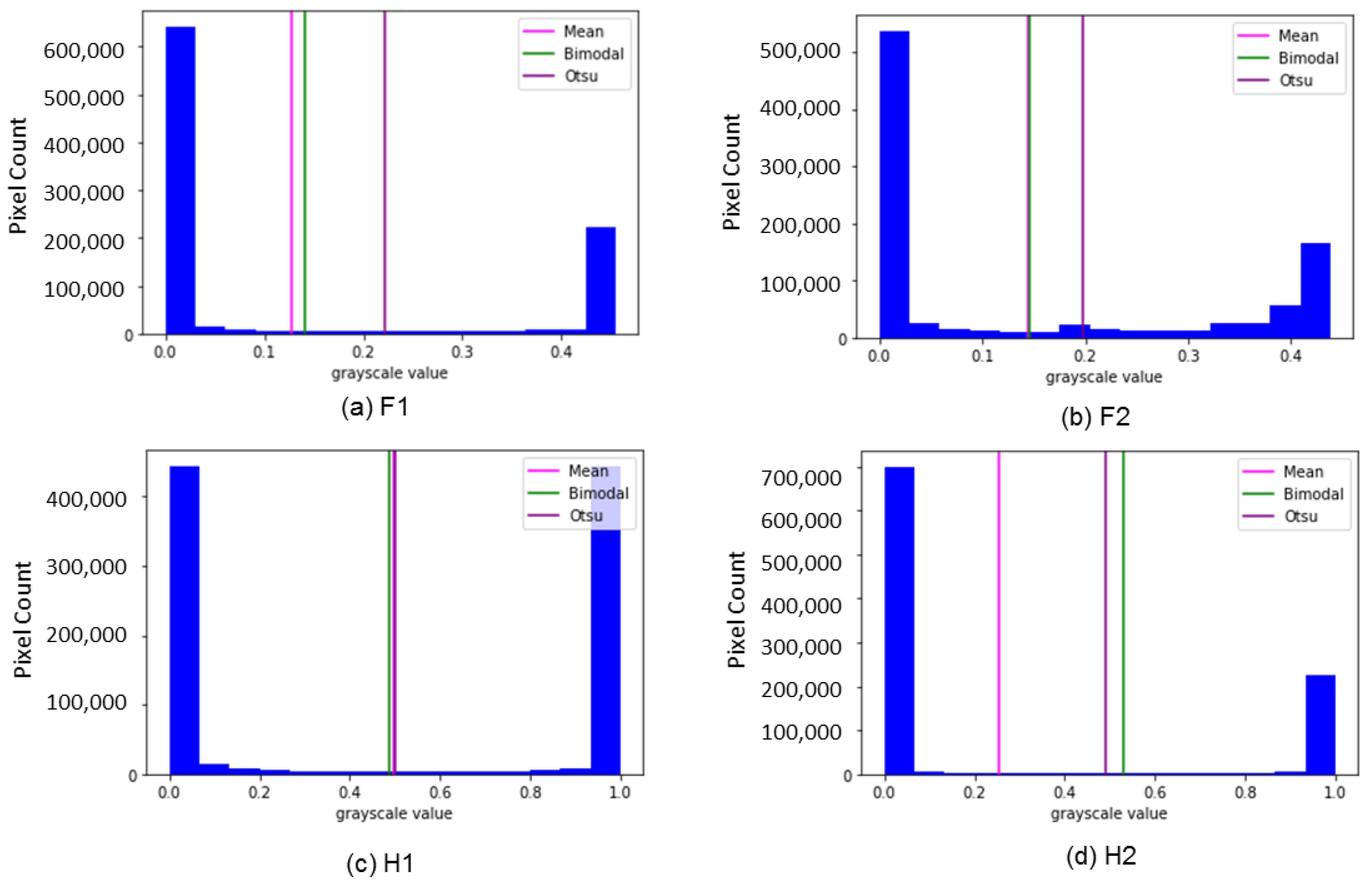
To classify and label each pixel from the model’s predicted output, which provided a probability of flooding ranging from 0 to 1, we experimented with various thresholding methods, including mean histogram, bimodal histogram, Otsu’s method, and 2-class k-means clustering. For the Florence flood, k-means clustering yielded binary flood maps with the highest evaluation scores across both test sites. Conversely, Otsu thresholding and mean histogram thresholding produced binary flood maps with the highest evaluation scores for H1 and H2, respectively. However, the differences in the f1 score for test sites F1, H1, and H2 were negligible, with less than a 1% variation, indicating that any of the tested binary classification methods could be effectively used (Table 3 and Table 4). Test site F2 exhibited a 3% difference in the f1 score between using k-means clustering (0.78) and mean and bimodal thresholding (0.75). As depicted in Figure 9, test site F2 presented a less distinct separation between the two peaks in the histogram. While histogram thresholding methods prove to be robust when a clear bimodal distribution exists, k-means does not rely on histograms for segmentation. Particularly, noise that is introduced in the image can be avoided by evaluating different pixels individually and grouping similar pixels together. Thus, in cases where the valley in the histogram was not as distinct, k-means clustering was recommended over histogram thresholding for binary classification.

Figure 9.
Histogram showing the pixel’s intensity of test sites (a–d) and their thresholding values.
Following the generation of a binary flood map using the aforementioned classification methods, Gaussian smoothing was then applied as a post-processing step. However, the results indicated that this step generally led to a decrease in most evaluation metrics, such as the precision, f1 score, IoU score, and accuracy, except for recall, albeit to a small extent. The primary objective of post-processing was to eliminate false positives and false negatives that the model failed to accurately classify, typically at a fine-grain level. However, the Gaussian filter employed for smoothing and noise removal introduced a blurring effect that was unhelpful in cases where the preservation of fine details was necessary.
5.3. Weakly Labeled Flood Map for Model Training Performance
Table 7 presents the performance comparison of the bi-temporal UNet model trained with the weakly labeled flood map generated from the proposed framework versus being trained with the manually labeled ground truth flood map for the Florence flood test sites F1 and F2. For site F1, the predicted flood map output (binarized with two-class k-means clustering) had better evaluation scores with the model being trained with the weakly labeled flood map. The Florence weakly labeled flood map obtained f1 scores of 77%, 87%, and 76% for the full-sized image, site F1, and site F2, respectively (Table 1), indicating the presence of noise or impurities in the map. While such noise existed, the f1 score of the weakly labeled flood map in site F1 (87%) was high enough such that machine learning models could still learn and filter out these noises, resulting in an improved predicted flood map with higher accuracy scores [43]. According to [43], if the labels in the training data were overly accurate (above a certain threshold), there were not enough noises and biases introduced to the model such that noises in the testing data could easily degrade the relationship learned by the models. In other words, the model became too localized to the training data and failed to generalize across new data, even within the same case study. However, if there is excessive noise or inaccuracy in the weakly labeled data, as seen in site F2 with an f1 score of 76%, the model may struggle to produce high-quality flood maps since machine learning techniques learn based on the frequency of patterns [43]. Consequently, hand-labeled annotations provided better model training than weak labels for site F2.

Table 7.
The performance of the bi-temporal UNet model when trained with the weakly labeled flood map from the proposed framework compared with the model when trained with the hand-labeled ground truth flood map for the Florence flood test sites F1 and F2.
A limitation of this weakly labeled generation process was that we only evaluated the framework with the Florence flood as we lacked hand-labeled annotations for the full-sized image of the Harvey flood (only available for Harvey test sites H1 and H2).
5.4. Bi-Temporal UNet Performance
The proposed bi-temporal UNet was trained using weakly labeled data that could be developed in near-real time. The performance of the model is demonstrated in Table 1 and Table 2, showcasing its effectiveness in urban flood mapping for both the Florence and Harvey study sites. These results highlight the model’s capability in near-real-time processing for future flooding events. The Florence study areas achieved an average f1 score of 0.836 and IoU score of 0.723, while the Harvey study areas achieved an average f1 score of 0.907 and an IoU score of 0.829. The evaluation scores for the Harvey flood study areas were higher than those for the Florence flood due to the larger amount of training data available.
Furthermore, the evaluation scores demonstrated the proposed framework’s transferability (i.e., generalizability) of new datasets associated with the heterogeneous image background. The model used a Dice BCE loss function (combination of Dice loss and standard binary cross-entropy loss) [44], allowing for some diversity in the loss from the Dice loss while benefitting from the stability provided by the BCE loss. The Dice loss also eliminated the need to define input weights during the algorithm’s initialization, even in the presence of class imbalance in the dataset.
The performance of the bi-temporal UNet was evaluated against other commonly used ML baseline models in flood mapping that also employed a bi-temporal (pre + post) input. The bi-temporal UNet outperformed these baseline models, on average, by 2.1% and 1.5% in sites H2 and H1, respectively. Notably, site H2 exhibited a higher degree of urbanization than site H1, which means site H2 had a more heterogeneous background. This indicates that the improvement in accuracy achieved by using the bi-temporal UNet over other baseline models with bi-temporal input was more pronounced in sites with greater heterogeneity. Similarly, the bi-temporal UNet outperformed the other models by 6.9% and 3.4% in sites F1 and F2, respectively, where site F1 was more urbanized than site F2. Consequently, the bi-temporal UNet demonstrated better performance compared with other models utilizing a bi-temporal input, particularly in sites characterized by a more heterogeneous background during each flood event.
5.5. Baseline Machine Learning Model Performances
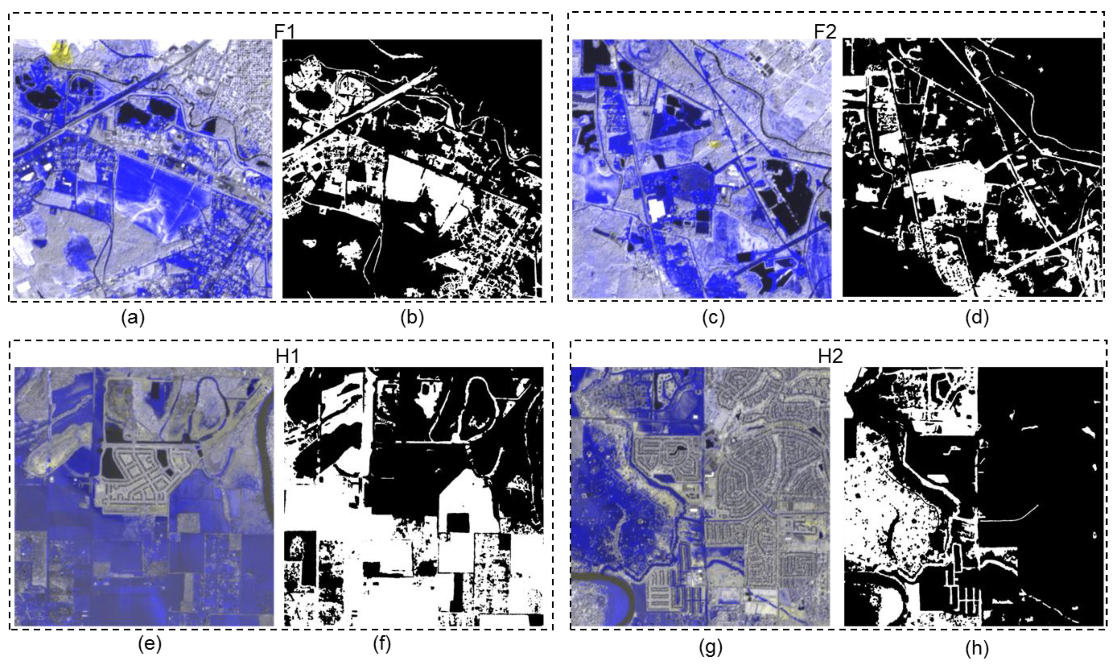
When comparing the performance of each model with bi-temporal input, DT, RF, and GBC showed similar results in their inability to accurately identify flooded pixels along the edges of flooded areas in site F1. Only AdaBoost misclassified two open water bodies as floodwater. DT had the highest number of false negatives, misclassifying flooded pixels not only around the edges but also within the flooded areas. However, in Figure 10a, it can be observed that there are mixed pixels within the center of the largest flooded area where the hand-labeled ground truth classifies as flooded pixels. Therefore, DT showed more sensitivity to mixed pixels compared with other models. In site F2, both DT and GBC were effective in distinguishing between open water bodies and floodwater, particularly in the top left and bottom right areas of the test site (Figure 10c). In site H1, the hand-labeled ground truth classified the heptagon area as flooded, whereas all models classified the top part of the heptagon as non-flooded (Figure 10e). GBC and AdaBoost exhibited greater sensitivity to these areas in site H1. Last, in site H2, the bi-temporal UNet and AdaBoost correctly classified the flooded area near the river bend in the bottom left area of the site (Figure 10g). Overall, DT and RF produced flood maps with the greatest similarity across all test sites. The bi-temporal UNet demonstrated the least sensitivity to mixed pixel areas, although this was dependent on the chosen threshold value during the binary classification stage. It is important to note that the evaluation of all models was dependent on the definition of flooded pixels in the hand-labeled annotations, which introduced a level of uncertainty due to potential human error.
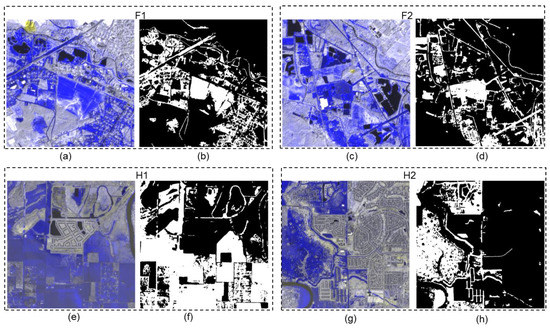
Figure 10.
False composition of test sites to show the difference between the pre- and post-flood images reflected in the NIR band by overlaying the NIR band of the post-flood to the NIR band of the pre-flood for test sites (a) F1, (c) F2, (e) H1, and (g) H2 compared with the hand-labeled ground truths for sites (b) F1, (d) F2, (f) H1, and (h) H2. The blue pixels in the false color composition images mark the changes in one direction (subtraction of pixel reflectance value that may be due to water or something of similar reflectance value like shadow), capturing the flooded change in the NIR bands of the pre- and post-flood images. The yellow pixels indicate the changes in another direction (addition of pixel reflectance value that may be due to addition of building, removal of grass, etc.). The gray pixels represent no change. The white pixels in the hand-labeled ground truth images represent flooded pixels. The black pixels represent the permanent water bodies in the false color composites, and non-flooded pixels in the flood map.
Although the bi-temporal UNet outperformed the baseline models (DT, RF, GBC, and AdaBoost) experimented on in this study across study sites F1, H1, and H2, except for site F2, for all input types (post-only and pre + post), future research could explore bi-temporal implementations of other deep learning models for flood mapping.
6. Conclusions and Future Work
This study proposed a framework to obtain a weakly labeled flood mask for model training and to generate a flood map that utilized bi-temporal data. The proposed framework was evaluated with commonly used baseline machine learning models (DT, RF, GBC, and AdaBoost) for flood extent mapping. The methodology involved generating a weakly labeled flood map through traditional RS (NDWI and change detection) and image processing (Canny edge detection) techniques to train the bi-temporal UNet model for flood detection. In the process of generating the weakly labeled flood mask, we introduced a noise removal method through Canny edge detection in combination with morphological operations and Gaussian smoothing.
Disaster response requires near-real-time actions from first responders. The availability of labels for modeling training and generalizability (or transferability) of a flood mapping model plays a critical role in real-time disaster response. Since it takes only negligible time (i.e., 2 min) to generate weak labels for each flood event, the proposed framework provides the capability for real-time flood mapping model training at a large scale. In addition, this work proved to be efficient in mapping floods over various highly heterogeneous built areas (e.g., residential, commercial, and industrial areas) for both the Florence flood and the Harvey flood (Table 2), demonstrating its generalizability and potentials to enable real-time flood mapping in a wide range of geographic environments.
The main limitations of this work are about the uncertainty in weak labels and ML and the explainability of ML models. In particular, weak labels can contain biases or noise in the training data and may lead to the amplification of those biases in the ML models’ predictions. In addition, the weak labels were only assessed using the Florence flood dataset as hand-labeled annotations for the full-sized image of the Harvey flood were unavailable, except for the Harvey test sites H1 and H2. Therefore, the evaluation of the framework’s performance was limited to the available annotations, and a comprehensive analysis incorporating the complete Harvey flood dataset was not feasible. Furthermore, the output flood maps predicted by ML models were not directly explainable. For example, the average evaluation score across all models with bi-temporal input was 2.9% greater than that of models with a uni-temporal input for both sites H1 and H2, despite site H2 being more urbanized or heterogenous than site H1 (Section 5.1). For the Florence flood, the bi-temporal models performed an average of 17.1% and 10.4% better than the uni-temporal models for sites F2 and F1, respectively, where site F2 was less heterogenous than site F1.
Accordingly, the future work can be focused on the following research directions to address these limitations and further enhance the current work:
- ML explainability examination: The effectiveness of machine learning (ML) models in flood mapping is expected to be largely influenced by the spatial and spectral heterogeneity of RS data, which captures the urban structure and level of urbanization in a study area. By quantifying the heterogeneity of RS data and examining its influence on ML-based flood mapping, we can gain insights into the performance of ML models and improve their explainability.
- Uncertainties in weak labels and ML: The performances of ML models are highly dependent on the accuracy of labels for training. While the proposed weak label generation framework can generalize to different geographic environments for producing training data corresponding to each flood event, noisy labels resulting from the framework can misguide the learning process. Uncertainty analysis can help understand the impact of various factors (e.g., noisy labels and model errors) on the performance of ML models. Quantifying and managing uncertainty can aid in selected ML models that generalize well for various locations and also provide valuable insights into ML explainability. In addition, different techniques, such as bootstrapping [45] and modifications of model architecture [46], can be explored to address the impact of weak labels and to mitigate their effects in ML models. Furthermore, formal methods, which use mathematical models to specify, build, and verify software and hardware systems, could also be leveraged for the verification and validation of the ML system [47,48].
- Weak label generation improvement: RS data consist of abundant spatial, temporal, and spectral information, which has a great potential for automatic weak label generation. This work enables weak labeling based on spectral and temporal information through traditional RS (NDWI and change detection) and image processing (Canny edge detection) techniques. Meanwhile, different auxiliary spatial data can aid in sampling weak labels, such as the FEMA national flood hazard layer (NFHL) and the building footprints. In particular, the FEMA NFHL is a geospatial dataset consisting of the U.S. national flood hazard data, indicating the annual probability of flooding, the flood way, and the flood zone. Building footprints can also be used to narrow down the geographic extent for sampling flooded and non-flooded areas as weak labels since most buildings are not likely to be submerged by floods. As such, we may further investigate the fusion of spatial, temporal, and spectral information for ground truth label generation and large-scale weakly supervised pixel-wise flood mapping in future.
- Flood mapping model enhancement: Although our proposed framework yielded the best results compared with other baseline models, there were still many false positives present in our output. With the f1 score being around 87%, we plan to experiment with pixel-wise data augmentation techniques, such as adding random shadows, to reduce the number of false positives. Additionally, we intend to conduct research and experiment with other model architectures for image segmentation that utilize bi-temporal input. Furthermore, we will investigate the inclusion of additional input information, such as characteristics of other ground objects and elevation data, to enhance the accuracy of water extraction.
Author Contributions
Conceptualization, J.V., Q.H. and B.P.; methodology, J.V., B.P. and Q.H.; software, J.V. and B.P.; validation, J.V.; formal analysis, J.V.; investigation, J.V.; resources, Q.H.; data curation, J.V. and B.P.; writing—original draft preparation, J.V.; writing—review and editing, J.V., Q.H., B.P., M.W. and C.G.A.; visualization, J.V.; supervision, Q.H.; project administration, Q.H.; funding acquisition, Q.H. All authors have read and agreed to the published version of the manuscript.
Funding
This research was funded by the National Science Foundation (No. 1940091) and the National Institute of Food and Agriculture (No. 1028199). Any opinions, findings, and conclusions or recommendations expressed in this material are those of the author(s) and do not necessarily reflect the views of the funders.
Data Availability Statement
The data and source code presented in this study are available at the following repository: https://github.com/vongkusolkit/bitemporalUNet, accessed on 29 May 2023.
Conflicts of Interest
The authors declare no conflict of interest.
References
- Tabari, H. Climate change impact on flood and extreme precipitation increases with water availability. Sci. Rep. 2020, 10, 13768. [Google Scholar] [CrossRef] [PubMed]
- National Research Council. Mapping the Zone: Improving Flood Map Accuracy; National Academies Press: Washington, DC, USA, 2009. [Google Scholar]
- Lorenzo-Alonso, A.; Utanda, Á.; Aulló-Maestro, M.E.; Palacios, M. Earth observation actionable information supporting disaster risk reduction efforts in a sustainable development framework. Remote Sens. 2018, 11, 49. [Google Scholar] [CrossRef]
- Olthof, I.; Tolszczuk-Leclerc, S. Comparing Landsat and RADARSAT for current and historical dynamic flood mapping. Remote Sens. 2018, 10, 780. [Google Scholar] [CrossRef]
- Ireland, G.; Volpi, M.; Petropoulos, G.P. Examining the capability of supervised machine learning classifiers in extracting flooded areas from Landsat TM imagery: A case study from a Mediterranean flood. Remote Sens. 2015, 7, 3372–3399. [Google Scholar] [CrossRef]
- Malinowski, R.; Groom, G.; Schwanghart, W.; Heckrath, G. Detection and delineation of localized flooding from WorldView-2 multispectral data. Remote Sens. 2015, 7, 14853–14875. [Google Scholar] [CrossRef]
- Feng, Q.; Liu, J.; Gong, J. Urban flood mapping based on unmanned aerial vehicle remote sensing and random forest classifier—A case of Yuyao, China. Water 2015, 7, 1437–1455. [Google Scholar] [CrossRef]
- Xie, M.; Jiang, Z.; Sainju, A.M. Geographical hidden markov tree for flood extent mapping. In Proceedings of the 24th ACM SIGKDD International Conference on Knowledge Discovery & Data Mining, London, UK, 19–23 August 2018; ACM: New York, NY, USA, 2018. [Google Scholar]
- Lim, J.; Lee, K.-s. Flood mapping using multi-source remotely sensed data and logistic regression in the heterogeneous mountainous regions in North Korea. Remote Sens. 2018, 10, 1036. [Google Scholar] [CrossRef]
- LeCun, Y.; Bengio, Y.; Hinton, G. Deep learning. Nature 2015, 521, 436. [Google Scholar] [CrossRef]
- Gebrehiwot, A.; Hashemi-Beni, L.; Thompson, G.; Kordjamshidi, P.; Langan, T.E. Deep convolutional neural network for flood extent mapping using unmanned aerial vehicles data. Sensors 2019, 19, 1486. [Google Scholar] [CrossRef]
- Ronneberger, O.; Fischer, P.; Brox, T. U-net: Convolutional networks for biomedical image segmentation. In Proceedings of the International Conference on Medical Image Computing and Computer-Assisted Intervention, Munich, Germany, 5–9 October 2015; Springer: Cham, Switzerland, 2015. [Google Scholar]
- Liu, X.; Deng, Z.; Yang, Y. Recent progress in semantic image segmentation. Artif. Intell. Rev. 2019, 52, 1089–1106. [Google Scholar] [CrossRef]
- Chen, T.; Kornblith, S.; Norouzi, M.; Hinton, G. A simple framework for contrastive learning of visual representations. In Proceedings of the International Conference on Machine Learning, PMLR, Virtual Event, 13–18 July 2020. [Google Scholar]
- He, K.; Fan, H.; Wu, Y.; Xie, S.; Girshick, R. Momentum contrast for unsupervised visual representation learning. In Proceedings of the IEEE/CVF Conference on Computer Vision and Pattern Recognition, Seattle, WA, USA, 13–19 June 2020. [Google Scholar]
- Peng, B.; Huang, Q.; Rao, J. Spatiotemporal Contrastive Representation Learning for Building Damage Classification. In Proceedings of the 2021 IEEE International Geoscience and Remote Sensing Symposium (IGARSS), Brussels, Belgium, 11–16 July 2021. [Google Scholar]
- Peng, B.; Huang, Q.; Vongkusolkit, J.; Gao, S.; Wright, D.B.; Fang, Z.N.; Qiang, Y. Urban Flood Mapping With Bitemporal Multispectral Imagery Via a Self-Supervised Learning Framework. IEEE J. Sel. Top. Appl. Earth Obs. Remote Sens. 2020, 14, 2001–2016. [Google Scholar] [CrossRef]
- Liu, X.; Sahli, H.; Meng, Y.; Huang, Q.; Lin, L. Flood inundation mapping from optical satellite images using spatiotemporal context learning and modest AdaBoost. Remote Sens. 2017, 9, 617. [Google Scholar] [CrossRef]
- Longbotham, N.; Pacifici, F.; Glenn, T.; Zare, A.; Volpi, M.; Tuia, D.; Christophe, E.; Michel, J.; Inglada, J.; Chanussot, J. Multi-modal change detection, application to the detection of flooded areas: Outcome of the 2009–2010 data fusion contest. IEEE J. Sel. Top. Appl. Earth Obs. Remote Sens. 2012, 5, 331–342. [Google Scholar] [CrossRef]
- Wieland, M.; Li, Y.; Martinis, S. Multi-sensor cloud and cloud shadow segmentation with a convolutional neural network. Remote Sens. Environ. 2019, 230, 111203. [Google Scholar] [CrossRef]
- Kwak, Y.-j. Nationwide flood monitoring for disaster risk reduction using multiple satellite data. ISPRS Int. J. Geo-Inf. 2017, 6, 203. [Google Scholar] [CrossRef]
- Ouma, Y.O.; Tateishi, R. A water index for rapid mapping of shoreline changes of five East African Rift Valley lakes: An empirical analysis using Landsat TM and ETM+ data. Int. J. Remote Sens. 2006, 27, 3153–3181. [Google Scholar] [CrossRef]
- Rosser, J.F.; Leibovici, D.; Jackson, M. Rapid flood inundation mapping using social media, remote sensing and topographic data. Nat. Hazards 2017, 87, 103–120. [Google Scholar] [CrossRef]
- Sivanpillai, R.; Jacobs, K.M.; Mattilio, C.M.; Piskorski, E.V. Rapid flood inundation mapping by differencing water indices from pre-and post-flood Landsat images. Front. Earth Sci. 2021, 15, 1–11. [Google Scholar] [CrossRef]
- McFeeters, S.K. The use of the Normalized Difference Water Index (NDWI) in the delineation of open water features. Int. J. Remote Sens. 1996, 17, 1425–1432. [Google Scholar] [CrossRef]
- Xu, H. Modification of normalised difference water index (NDWI) to enhance open water features in remotely sensed imagery. Int. J. Remote Sens. 2006, 27, 3025–3033. [Google Scholar] [CrossRef]
- Feyisa, G.L.; Meilby, H.; Fensholt, R.; Proud, S.R. Automated Water Extraction Index: A new technique for surface water mapping using Landsat imagery. Remote Sens. Environ. 2014, 140, 23–35. [Google Scholar] [CrossRef]
- Zhang, Q.; Jindapetch, N.; Buranapanichkit, D. Investigation of image edge detection techniques based flood monitoring in real-time. In Proceedings of the 2019 16th International Conference on Electrical Engineering/Electronics, Computer, Telecommunications and Information Technology (ECTI-CON), Pattaya, Thailand, 10–13 July 2019; IEEE: Piscataway, NJ, USA, 2019. [Google Scholar]
- Ghandorh, H.; Boulila, W.; Masood, S.; Koubaa, A.; Ahmed, F.; Ahmad, J. Semantic segmentation and edge detection—Approach to road detection in very high resolution satellite images. Remote Sens. 2022, 14, 613. [Google Scholar] [CrossRef]
- Billa, L.; Pradhan, B. Semi-automated procedures for shoreline extraction using single RADARSAT-1 SAR image. Estuar. Coast. Shelf Sci. 2011, 95, 395–400. [Google Scholar]
- Dhanachandra, N.; Manglem, K.; Chanu, Y.J. Image segmentation using K-means clustering algorithm and subtractive clustering algorithm. Procedia Comput. Sci. 2015, 54, 764–771. [Google Scholar] [CrossRef]
- Huang, M.; Yu, W.; Zhu, D. An improved image segmentation algorithm based on the Otsu method. In Proceedings of the 2012 13th ACIS International Conference on Software Engineering, Artificial Intelligence, Networking and Parallel/Distributed Computing, Washington, DC, USA, 8–10 August 2012; IEEE: Piscataway, NJ, USA, 2012. [Google Scholar]
- Jain, S.K.; Singh, R.; Jain, M.; Lohani, A. Delineation of flood-prone areas using remote sensing techniques. Water Resour. Manag. 2005, 19, 333–347. [Google Scholar] [CrossRef]
- Belgiu, M.; Drăguţ, L. Random forest in remote sensing: A review of applications and future directions. ISPRS J. Photogramm. Remote Sens. 2016, 114, 24–31. [Google Scholar] [CrossRef]
- Nandi, I.; Srivastava, P.K.; Shah, K. Floodplain mapping through support vector machine and optical/infrared images from Landsat 8 OLI/TIRS sensors: Case study from Varanasi. Water Resour. Manag. 2017, 31, 1157–1171. [Google Scholar] [CrossRef]
- Long, J.; Shelhamer, E.; Darrell, T. Fully convolutional networks for semantic segmentation. In Proceedings of the IEEE Conference on Computer Vision and Pattern Recognition, Boston, MA, USA, 7–12 June 2015. [Google Scholar]
- Li, Z.; Demir, I. U-net-based semantic classification for flood extent extraction using SAR imagery and GEE platform: A case study for 2019 central US flooding. Sci. Total Environ. 2023, 869, 161757. [Google Scholar] [CrossRef]
- Zhao, G.; Pang, B.; Xu, Z.; Peng, D.; Xu, L. Assessment of urban flood susceptibility using semi-supervised machine learning model. Sci. Total Environ. 2019, 659, 940–949. [Google Scholar] [CrossRef]
- Bonafilia, D.; Tellman, B.; Anderson, T.; Issenberg, E. Sen1Floods11: A georeferenced dataset to train and test deep learning flood algorithms for sentinel-1. In Proceedings of the IEEE/CVF Conference on Computer Vision and Pattern Recognition Workshops, Seattle, WA, USA, 14–19 June 2020. [Google Scholar]
- Powers, D.M. Evaluation: From precision, recall and F-measure to ROC, informedness, markedness and correlation. arXiv 2020, arXiv:2010.16061. [Google Scholar]
- Tehrany, M.S.; Pradhan, B.; Mansor, S.; Ahmad, N. Flood susceptibility assessment using GIS-based support vector machine model with different kernel types. Catena 2015, 125, 91–101. [Google Scholar] [CrossRef]
- Najafzadeh, M.; Basirian, S. Evaluation of River Water Quality Index Using Remote Sensing and Artificial Intelligence Models. Remote Sens. 2023, 15, 2359. [Google Scholar] [CrossRef]
- Liu, X.; Zhu, A.-X.; Yang, L.; Pei, T.; Qi, F.; Liu, J.; Wang, D.; Zeng, C.; Ma, T. Influence of legacy soil map accuracy on soil map updating with data mining methods. Geoderma 2022, 416, 115802. [Google Scholar] [CrossRef]
- Jadon, S. A survey of loss functions for semantic segmentation. In Proceedings of the 2020 IEEE Conference on Computational Intelligence in Bioinformatics and Computational Biology (CIBCB), Vina del Mar, Chile, 27–29 October 2020; IEEE: Piscataway, NJ, USA, 2020. [Google Scholar]
- Reed, S.; Lee, H.; Anguelov, D.; Szegedy, C.; Erhan, D.; Rabinovich, A. Training deep neural networks on noisy labels with bootstrapping. arXiv 2014, arXiv:1412.6596. [Google Scholar]
- Sukhbaatar, S.; Bruna, J.; Paluri, M.; Bourdev, L.; Fergus, R. Training convolutional networks with noisy labels. arXiv 2014, arXiv:1406.2080. [Google Scholar]
- Krichen, M.; Mihoub, A.; Alzahrani, M.Y.; Adoni, W.Y.H.; Nahhal, T. Are Formal Methods Applicable To Machine Learning And Artificial Intelligence? Proceedings of the 2022 2nd International Conference of Smart Systems and Emerging Technologies (SMARTTECH), Riyadh, Saudi Arabia, 9–11 May 2022. IEEE: Piscataway, NJ, USA, 2022. [Google Scholar]
- Raman, R.; Gupta, N.; Jeppu, Y. Framework for Formal Verification of Machine Learning Based Complex System-of-Systems. Insight 2023, 26, 91–102. [Google Scholar] [CrossRef]
Disclaimer/Publisher’s Note: The statements, opinions and data contained in all publications are solely those of the individual author(s) and contributor(s) and not of MDPI and/or the editor(s). MDPI and/or the editor(s) disclaim responsibility for any injury to people or property resulting from any ideas, methods, instructions or products referred to in the content. |
© 2023 by the authors. Licensee MDPI, Basel, Switzerland. This article is an open access article distributed under the terms and conditions of the Creative Commons Attribution (CC BY) license (https://creativecommons.org/licenses/by/4.0/).

