Abstract
To achieve river channel detection in SAR (synthetic aperture radar) images, we developed a level-set-based model (LSBM) guided by a designed data-fitting energy which is called the SoDEF (sum of dual exponential functions)-fitting energy. Firstly, we designed a function by computing the sum of dual exponential functions to substitute for the quadratic function, and used it to construct the data-fitting energy. Secondly, the adaptive area-fitting centers (AFCs) were computed based on two kinds of grayscale characteristics, which are more accurate and more stable. Thirdly, the Dirac function in gradient descent flow was displaced by an edge indicator function to help the evolving level sets stop at the target edges. Moreover, some regularized terms were incorporated into the objective function to guarantee the model’s stability. The river channel detection experiments conducted with real SAR images indicated that the developed model is superior to the related state-of-the-art methods in its detection accuracy and efficiency.
1. Introduction
River channel detection has a clear benefit for numerous practical applications of water resources protection, geological environment exploration, bridge and dam construction, aquaculture industry planning, water transportation management, etc. In the past, this task was carried out manually, which involved significant costs and time. Additionally, its detection accuracy cannot be guaranteed. In view of the development and maturity of remote sensing imaging technology, especially SAR imaging, which has the characteristics of operating all day and in all weather, this approach has become one of the major methods used for ground target detection. In the process of achieving the above purpose, image segmentation is the key step. Therefore, we concentrated on the segmentation of SAR river images to detect river channels.
For the last few years, level-set-based models (LSBMs) [1,2,3,4] played a key role in the tasks of image segmentation due to their advantages, namely convenient modeling, easy programming, and efficient computation. Currently, LSBMs can essentially be divided into three categories: local characteristic-based LSBMs (LCLSBMs) [5,6,7,8], global characteristic-based LSBMs (GCLSBMs) [9,10,11,12], and hybrid characteristic-based LSBMs (HCLSBMs) [13,14,15,16]. GCLSBMs usually draw on global characteristics of images, such as the global inter-class variance (ICV) [17], global coefficient of variation [18], global area descriptor [19], global area-based pressure force [20], and so on, to guide the level sets; they are successful in segmenting images with homogeneous pixels. Additionally, these models involve relatively low computational complexities. The well-known Chan–Vese (CV) [21] model is a typical case, which is built based on the two piecewise functions. This model computes the global ICVs of pixel grayscales inside and outside the level sets to control the model’s evolution, and obtains ideal segmentation results for images with simple homogeneous scenes. However, its construction has a hypothetical premise, i.e., the target image only contains two homogeneous areas, which causes the CV model to fail to process images with complicated scenes. Subudhi et al. [22] proposed a novel GCLSBM based on the coefficient of variation and graph-cut optimization (CVGCO). The CVGCO model first computes the global coefficient of variation inside and outside the level sets as global statistics, and the local patch coefficient of variation inside and outside the level sets as local statistics. Then, its data-guided energy term can be obtained by comparing the differences between the global and local statistics. Moreover, graph-cut optimization is incorporated to implement this model, which achieves less sensitivity to level-set re-initialization. Consequently, the CVGCO model is capable of handling images with complex pixels. To summarize, GCLSBMs [23,24] are highly suitable for segmenting images with homogeneous pixels, and perform with relatively high efficiencies. However, these models have difficulties in processing images with non-homogeneous pixels.
To tackle the above issues, LCLSBMs have been developed that utilize local characteristics of images, such as local fractional order differentiation [25], local inter-class variance [26], local cosine-fitting energy [27], local approximation of Taylor expansion [28], and so on, to guide the level sets; they are competent for dealing with images with non-homogeneous pixels. Yang et al. [29] proposed a new LCLSBM using region-scalable fitting and atlas correcting information (RSFACI). This model first adopts the coherent local intensity clustering method to calculate the atlas correcting information, and then the atlas fitting term (AFT) is defined. Following this, the AFT is merged with the region-scalable fitting (RSF) term to construct the model’s data-guided energy. In addition, some regularization terms are introduced to smooth the level sets. The RSFACI model is applied to segmenting non-homogeneous medical images, and achieves some desirable results. Biswas et al. [30] put forward another new LCLSBM based on modified local region fitting (MLRF) and double-well potential (DWP) penalty energies. Firstly, a circle-window filter is utilized to obtain local region information, and the MLRF energy term is developed using that information. Secondly, a novel DWP function is designed for regularizing the level sets, which increases its smoothness. Furthermore, this DWP function is considered as the penalty energy term, and is incorporated into the above MLRF energy term. Finally, the MLRF-DWP model produces some satisfying segmentation results for multiple types of images with non-homogeneous pixels. In a word, LCLSBMs [31,32] are good at coping with images involving non-homogeneous pixels, and can obtain accurate local area targets. However, these models have some conspicuous flaws, i.e., they rely heavily on level set initialization, and their computational efficiencies are relatively low.
Considering merging the advantages of the former two LSBMs, researchers presented HCLSBMs, which draw upon hybrid characteristics of images to guide the level sets. Ozturk et al. [33] proposed a new HCLSBM that integrated the CV model with the LGDF (local Gaussian distribution fitting) model. In this model, the image segmentation task can be divided into two stages. The first-stage segmentation uses the global characteristics, namely the CV model, to rapidly extract homogeneous areas in the input image. Subsequently, the second-stage segmentation exploits the local characteristics, namely the LGDF model, to segment the non-homogeneous pixels of those areas. Eventually, the hybrid CV–LGDF model creates better segmentation performance than the CV and LGDF models alone. Han et al. [34] presented another HCLSBM driven by Jeffreys divergence fitting (JDF) energies. The JDF model first adopts Jeffreys divergence to construct the local characteristic-driven energy term, replacing the Euclidean distance in the RSF model. Second, the global characteristic-driven energy term is similarly constructed using Jeffreys divergence, which enhances the model’s segmentation ability. Moreover, the adaptive coefficients for adjusting local and global characteristic-driven energy terms are designed. Consequently, the JDF model efficiently yields some accurate segmentation for real-world and medical images. In conclusion, HCLSBMs [35,36] succeed in dealing with many types of images involving homogeneous and non-homogeneous pixels. However, they still need to input eligible initial level sets, and the automatic selection of local and global energy terms is also a difficult issue.
In recent years, researchers applied LSBMs to the segmentation of remote sensing images [37,38,39], especially for SAR images [40,41]. Liu et al. [42] put forward a novel LSBM based on reaction-diffusion energy (RDE) terms. This model firstly constructs the reaction energy term by fusing gamma statistical distribution and area–boundary characteristics, which can guide the level set evolution and repress speckle noise to some degree. Secondly, the diffusion energy term is incorporated to avoid level set re-initialization, which maintains the regularity of the segmented area. Therefore, the RDE model produces some desirable segmentation results of SAR images. Han et al. [43] developed an adaptive LSBM using weighted area-based signed pressure force (WABSPF) to process SAR images. Firstly, the normalized ICVs of pixel grayscales inside and outside the level sets are computed, which serve as the new weights of the AFCs, and then the WABSPF function is built. Afterwards, to obtain more accurate AFCs, the adaptive coefficients are incorporated in their calculation, which weakens the interference of noise. Moreover, some regularizing energies are introduced to stabilize the level set evolution. Consequently, the WABSPF model is capable of extracting target areas from SAR images. Although LSBMs have succeeded in segmenting SAR images and produced some good detection of targets, their performance still needs further improvement, especially in detection accuracy and efficiency.
In addition to the above-mentioned LSBMs, there are some other methods with applications to river channel detection. Shang et al. [44] presented a new target detection method in SAR images that uses fuzzy clustering algorithm and hierarchical segmentation (FCAHS). This method divides the image pixels into multiple sets, and chooses the core pixels in each set to obtain the thumbnails. Then, the fuzzy clustering algorithm is used to deal with these thumbnails. Finally, the target in SAR images is detected using hierarchical segmentation. However, the FCAHS method is not very capable of handling local target regions. Luo et al. [45] proposed an optimized ratio of exponentially weighted averages (OROEWA) edge-detecting function-based method to achieve SAR image target detection. The ROEWA is firstly adopted to calculate the edge strength map of the input SAR image. Thereafter, the curvilinear structure extraction approach is introduced to detect target edges substituting for watershed-algorithm or non-maximum suppression. Eventually, the OROEWA method can detect weak boundaries and guarantee its smoothness; however, it extracts many undesired boundaries in SAR images. Xu et al. [46] constructed a river channel detection framework based on the attention U-net and multi-scale LSBM (AUMLSBM). This framework firstly utilized the attention U-net to roughly detect river channels in the SAR image, and its detection results are considered as the initial level sets for subsequent refinement of the river channels. Then, the multi-scale LSBM is carried out to obtain better river channel detection. Unfortunately, the AUMLSBM is a supervised method that needs large SAR data sets. Furthermore, it only makes changes in the way the initial level sets are generated, which cannot significantly improve the detection performance. In summary, the above recent methods are unable to achieve satisfactory river channel detection in SAR images.
In this study, we developed a novel LSBM guided by SoDEF fitting energy to achieve accurate and rapid river channel detection in SAR images. The following are some of the main contributions:
- (1)
- A function called the SoDEF (Sum of Dual Exponential Functions) was designed and used to construct the data-fitting energy, guiding the level set evolution.
- (2)
- The adaptive AFCs were computed using two kinds of grayscale characteristics, which are more accurate and more stable.
- (3)
- An edge indicator function was incorporated to displace the Dirac function in gradient descent flow, which can encourage the evolving level sets to stop at the target edges.
The rest of this study is arranged as follows: In Section 2, we briefly recall the related LSBMs. In Section 3, the construction of the developed SoDEF model is described in detail. The corresponding experiments and analysis are discussed in Section 4. Finally, some conclusions are drawn in Section 5.
2. Background
2.1. The CV Model
Chan and Vese [21] made an assumption that an image u defined on the image domain can be classified into two homogeneous parts, which are represented with the mean values of pixel grayscales inside those two parts. Following this, a special case of the Mumford–Shah LSBM, which is termed as the CV model, is given. Hence, its objective energy function can be represented as:
where denotes the level set function, and represent regularizing Dirac and Heaviside functions, and λ represent related coefficients, and c1 and c2 represent mean AFCs, which can be calculated with the following:
Regarding c1 and c2 as the constants, the gradient descent method (GDM) was used for solving Equation (1), and its gradient descent flow (GDF) was obtained as follows:
The CV model is a GCLSBM, and shows good competence in processing images involving simple homogeneous pixels. Moreover, it is free for setting initial level sets. However, the CV model has trouble segmenting images with complex and non-homogeneous scenes. Therefore, it is not suitable for river channel detection.
2.2. The RSF Model
To process images involving non-homogeneous pixels, Li et al. [26] developed the RSF model, which calculates the local ICVs of pixel grayscales inside and outside the level sets, in order to control the model’s evolution. Thus, its objective energy function can be represented as the following:
where represents the region scalable factor, , and represent corresponding energy weights, and f1 and f2 represent local mean AFCs that can be computed with the following:
Regarding f1 and f2 as constants, Equation (4) can be resolved by the GDM, and its GDF is obtained as the following:
The RSF model is an LCLSBM, and succeeds in handling images with non-homogeneous pixels. However, its high computational complexity leads to expensive executive time. In addition, its segmentation effect is very dependent on the input level sets. In other words, the RSF model is incapable of detecting river channels in SAR images accurately.
3. Proposed Method
3.1. The SoDEF Fitting Energy Term
First, we remove the regularized energies in the CV and RSF models, and their data-fitting energy (DFE) terms are retained. Then, they can be rewritten as the following:
By observing Equation (7), the above DFE terms are actually quadratic-fitting energy terms, i.e., they are constructed based on the quadratic function . However, the evolution of the level sets guided by these DFE terms is not efficient, and this is because the quadratic-fitting energy is not strong [47]. Especially when the input image pixel grayscales are close to their AFCs, the guiding energies will be small, which causes the level sets to move slowly. In a word, the quadratic-fitting energy cannot perform an efficient level set evolution. Moreover, it has trouble dealing with areas with close grayscales.
To tackle the above issues, we designed a new function called the SoDEF, which was built by computing the sum of dual exponential functions. Therefore, it can be represented as the following:
Next, we make a comparison between and graphically, as shown in Figure 1.
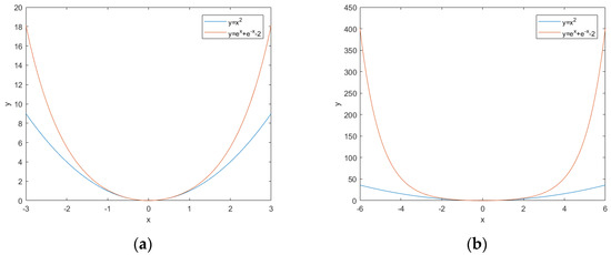
Figure 1.
Comparison of two functions; (a) x ranging from −3 to 3; (b) x ranging from −6 to 6.
According to Figure 1, there are some facts: (1) they are all convex functions, and can be solved by the GDM; (2) when the value of x is relatively small, the value of the SoDEF function is bigger than that of the quadratic function; (3) when the value of x is relatively large, the value of the SoDEF function is much bigger than that of the quadratic function.
In view of the above, a novel data-fitting energy term based on the SoDEF function was developed, and is represented as the following:
The SoDEF-fitting energy term performs more effectively than the quadratic-fitting energy term. Specifically, during the model’s evolution, it can produce much stronger energies to guide the level sets towards target edges more efficiently. In particular, when the input image pixel grayscales are close to their AFCs, the SoDEF-fitting energy term still provides sufficient energies to encourage the motion of level sets. Thus, it has the competence to handle areas with close grayscales.
3.2. The Adaptive AFCs
In the above SoDEF-fitting energy term and most DFE terms of existing LSBMs, the mean grayscale characteristics inside and outside the level sets, namely c1 and c2, are computed as the inner and outer AFCs. However, interference pixels such as noise and outlier pixels are associated with their computation directly, which decreases the accuracy of AFCs and affects the model’s segmentation competence. To surmount this difficulty, we first computed the median grayscale characteristics inside and outside the level sets as another kind of AFC, which can be represented as follows:
where m1 and m2 represent median AFCs.
The median AFCs are not greatly sensitive to interference pixels [48]; thus, their accuracies are better than the mean AFCs. However, they are not correct in a few extreme cases. To avoid this, we then constructed new adaptive AFCs based on the above two kinds of grayscale characteristics, that is, the mean and median AFCs; their calculation formulas are represented as follows:
where and represent adaptive AFCs, and are the adjustment coefficients, which can be calculated with the following:
The adaptive AFCs are more accurate and stable than the existing AFCs. More specifically, when the differences between median AFCs and mean AFCs are comparatively small, the adjustment coefficients are small. Thus, the median AFCs occupy larger proportions of the adaptive AFCs, which makes adaptive AFCs more accurate, and the model proposed can produce better performance. In contrast, when the differences between the median AFCs and mean AFCs are comparatively large, the adjustment coefficients are large. Therefore, the mean AFCs occupy larger proportions of the adaptive AFCs. Especially when these differences are extremely large, the mean AFCs will play the dominant role, which can restrain the case of incorrect median AFCs and ensure the stability of adaptive AFCs. Consequently, the developed adaptive AFCs are more accurate and stable than the existing AFCs, and create better segmentation competence.
Next, we used the adaptive AFCs to substitute for the mean AFCs in the SoDEF-fitting term. Hence, the SoDEF-fitting term with adaptive AFCs can be represented as the following:
3.3. The Improved Gradient Descent Flow
To further guarantee the stability of the level set evolution, two normally used regularized energies are introduced into the above DFE term, and they are computed by the following:
where and represent length-regularized and penalty-regularized energies, respectively.
Therefore, the total objective energy function of the proposed method can be represented as follows:
Regarding and as constants, Equation (16) can be solved by the GDM, and its GDF is obtained as the following:
During the level set evolution, in Equation (17) is approximated to a pulse function, and its values are close to one near the level sets while other values are close to zero; this is not beneficial for dealing with pixels that are far away from the level sets. Therefore, we used an edge indicator function to displace to overcome the above problem. The edge indicator function g is constructed as follows:
where l represents the Laplacian of the Gaussian (LoG) response diagram of the input image, and ρ is a ratio constant. In addition, l can be computed with the following:
where represents a Gaussian kernel function, and is the input image.
Based on Equation (18), when the evolving level sets locate near the target edges, the value of l is large and the value of g is small, which tends to zero. This helps the evolving level sets stop at the target edges. Finally, the improved GDF of the SoDEF model can be represented as the following:
3.4. Advantages and Algorithm Implementation of the SoDEF Model
In view of the above, we sum up the advantages of the proposed method as shown below:
- (1)
- The SoDEF model can achieve better segmentation competence.
In the proposed method, the level set evolution is guided by the SoDEF-fitting energy instead of the quadratic-fitting energy, which is more applicable. Even when the input image pixel grayscales are close to their AFCs, it can still provide sufficient energies to guide the level sets. Thus, it has the ability to process areas with close grayscales. Moreover, the new adaptive AFCs are used to replace the existing mean AFCs, and they can inhibit interference pixels to some degree, making them more accurate and stable. Consequently, the SoDEF model can create better segmentation performance.
- (2)
- The SoDEF model can obtain high executive efficiency.
During the level set evolution, the SoDEF-fitting energy term produces much stronger energies to guide the level sets towards the target edges, which is more efficient than the quadratic-fitting energy term. In addition, a LoG-based edge indicator is constructed, and is utilized to displace the Dirac function in the GDF of the proposed method. It is able to help the evolving level sets stop at the target edges. Due to the above factors, the SoDEF performs well in executive efficiency.
Following this, we utilize the finite difference method to solve the final GDF numerically. The specific implementation process of the SoDEF model is illustrated in Figure 2.
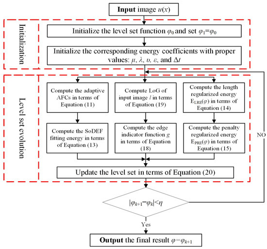
Figure 2.
The implementation flowchart of the SoDEF model.
4. Experimental Results and Analysis
In this part, the SoDEF model was utilized to detect river channels in different types of SAR images. Its detection results were compared to those of some corresponding LSBMs, i.e., the CV, CVGCO, RSFACI, JDF, RDE, and WABSPF models, as well as other recent river channel detection methods, namely the FCAHS and AUMLSBM methods, in order to prove its effectiveness and advantages. All of the experiments were carried out on a laptop with the following specifications: Intel Core i7-9750H, 2.60GHz, 16GB-RAM, MATLAB-R2017a, Windows 10. The related experimental coefficients of above methods are shown in Table 1.

Table 1.
Related coefficients of experimental methods.
4.1. Detected River Channels from Real SAR Images of Different Methods
The corresponding river channel detection results of the above nine methods are shown in Figure 3, Figure 4, Figure 5, Figure 6, Figure 7, Figure 8, Figure 9 and Figure 10.
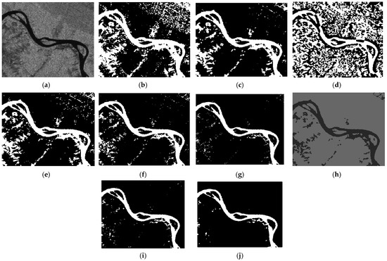
Figure 3.
River channel detection results of SAR image 1 by seven LSBMs. (a) is an input SAR image, (b–j) are the results of the CV, CVGCO, RSFACI, JDF, RDE, WABSPF, FCAHS, AUMLSBM, and SoDEF methods, respectively.
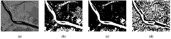
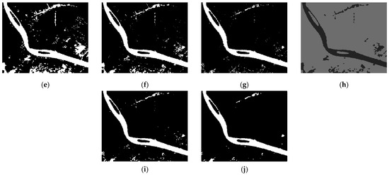
Figure 4.
River channel detection results of SAR image 2 by seven LSBMs. (a) is an input SAR image, (b–j) are results of the CV, CVGCO, RSFACI, JDF, RDE, WABSPF, FCAHS, AUMLSBM, and SoDEF methods, respectively.
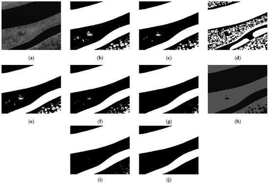
Figure 5.
River channel detection results of SAR image 3 by seven LSBMs. (a) is an input SAR image, (b–j) are results of the CV, CVGCO, RSFACI, JDF, RDE, WABSPF, FCAHS, AUMLSBM, and SoDEF methods, respectively.
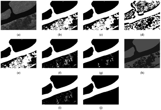
Figure 6.
River channel detection results of SAR image 4 by seven LSBMs. (a) is an input SAR image, (b–j) are results of the CV, CVGCO, RSFACI, JDF, RDE, WABSPF, FCAHS, AUMLSBM, and SoDEF methods, respectively.
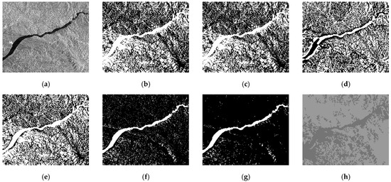
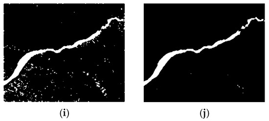
Figure 7.
River channel detection results of SAR image 5 by seven LSBMs. (a) is an input SAR image, (b–j) are results of the CV, CVGCO, RSFACI, JDF, RDE, WABSPF, FCAHS, AUMLSBM, and SoDEF methods, respectively.
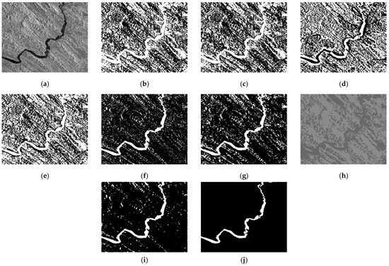
Figure 8.
River channel detection results of SAR image 6 by seven LSBMs. (a) is an input SAR image, (b–j) are results of the CV, CVGCO, RSFACI, JDF, RDE, WABSPF, FCAHS, AUMLSBM, and SoDEF methods, respectively.
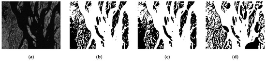
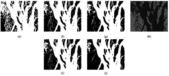
Figure 9.
River channel detection results of SAR image 7 by seven LSBMs. (a) is an input SAR image, (b–j) are results of the CV, CVGCO, RSFACI, JDF, RDE, WABSPF, FCAHS, AUMLSBM, and SoDEF methods, respectively.
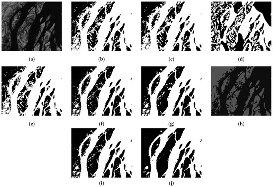
Figure 10.
River channel detection results of SAR image 8 by seven LSBMs. (a) is an input SAR image, (b–j) are results of the CV, CVGCO, RSFACI, JDF, RDE, WABSPF, FCAHS, AUMLSBM, and SoDEF methods, respectively.
According to Figure 3, Figure 4, Figure 5, Figure 6, Figure 7, Figure 8, Figure 9 and Figure 10, we know that both GCLSBMs, namely the CV and CVGCO models, cannot achieve good river channel detection, and many pixels are wrongly identified as river channels, which leads to bad detection accuracy. The detected river channels of the RSFACI model are even worse. There exist many more wrongly detected pixels in its detection results. The JDF model performed slightly better than the previous LSBMs. Its detection accuracy improved a little, which is not significant. In regard to the specific LSBMs for dealing with SAR images, namely the RDE and WABSPF models, their detected results are much more accurate than the above experimental LSBMs. In particular, the WABSPF model showed good detection performance; however, its detection accuracy is not satisfactory. The FCAHS method obtained detection results that were similar to the GCLSBMs, and the AUMLSBM resulted in a detection performance tht was close to the WABSPF model. The developed LSBM, namely the SoDEF model, produced the best detection results, and the river channels that it detected were the most accurate and cleanest, with few non-river pixels. Therefore, the detection performance of the SoDEF model is superior to that of the other experimental LSBMs.
4.2. Comparison with State-of-the-Art Methods and Related Quantitative Evaluation
In light of the above river channel detected results for different types of SAR images, we can see that the SoDEF model outperformed the state-of-the-art methods in detection accuracy. This was analyzed specifically as follows:
- (1)
- The CV model [21] is guided by the quadratic-fitting energies, and when the input image pixel grayscales are close to their AFCs, its guiding energies are small; this leads to trouble in processing areas with close grayscales. Thus, many non-target areas whose grayscales are similar to river channels are mistaken for the target areas.
- (2)
- The CVGCO model [22] computes the global coefficient of variation inside and outside the level sets as global statistics, and the local patch coefficient of variation inside and outside the level sets as local statistics. Then, it compares the differences between the global and local statistics to segment the images. However, those statistics cannot describe SAR river images well, which results in bad detection performance.
- (3)
- The RSFACI model [29] combines the region-scalable fitting term with the atlas fitting term to guide the level sets. Actually, it is mainly guided by the local quadratic-fitting energies, which extract many local details. In addition, edge leakage happens in the detected results. Therefore, the RSFACI model produced the worst detection effect.
- (4)
- The JDF model [34] exploits both local and global Jeffreys divergence-fitting energies to drive the level sets, and designs the adaptive coefficients for automatically adjusting the global and local energies. Hence, it achieved relatively better detection results than the former three LSBMs. Unfortunately, this improvement is far from satisfactory.
- (5)
- The RDE model [42] draws upon two kinds of energies, namely the reaction and diffusion energies, to guide the level sets. The reaction energy is constructed using gamma statistical distribution and area–boundary features, which inhibits interference noise to some extent. Moreover, its diffusion energy can refrain from re-initializing the level sets. Therefore, the RDE achieved some good detection results.
- (6)
- The WABSPF model [43] first utilizes the normalized ICVs of pixel grayscales inside and outside the level sets to build the WABSPF function, which can dominate the level set evolution better. Then, the adaptive coefficients are introduced into the calculation of its AFCs, which weakens the interference of noise. Consequently, it is capable of achieving better detection results than the RDE model. However, the detection accuracies of both the RDE and WABSPF models are still undesired, and still need further enhancement.
- (7)
- The FCAHS method [44] exploits the fuzzy clustering algorithm to process the obtained thumbnails, and detects the targets in SAR images based on hierarchical segmentation. Actually, this method depends on grayscale characteristics to detect river channels; therefore, many of the non-river regions were wrongly detected.
- (8)
- The AUMLSBM method [46] firstly utilizes the attention U-net to roughly segment SAR images, in order to generate the initial level sets for the subsequent detection of river channels. Then, the multi-scale LSBM is used to refine the regions of river channels. However, it only optimizes the initial conditions of the method, which cannot obviously improve the detection performance.
- (9)
- The developed LSBM is guided by the SoDEF-fitting energies substituting for the quadratic-fitting energies. It can provide much stronger energies to guide the level set evolution, which leads to higher executive efficiency, and makes the model achieve the competence to process areas with close grayscales. Moreover, the adaptive AFCs were designed with two kinds of grayscale characteristics, which can repress the effect of interference pixels. Thus, they are more accurate and stable than common mean AFCs, which creates a better detection ability. Additionally, the Dirac function in the GDF is displaced by a LoG-based edge indicator to help the evolving level sets stop at the target edges. Consequently, the SoDEF model was capable of detecting river channels in the SAR images most accurately, and produced the best detection performance.
Following this, the related quantitative evaluations of the above-mentioned detection results by the nine experimental methods were conducted to analyze the detection performance objectively on the basis of two indices, accuracy (QA) and false alarm (QFA), which can be calculated by the following:
where Tp denotes the rightly detected river channel grayscales, Fp denotes the falsely detected river channel grayscales, Tn denotes the correctly detected background grayscales, and Fn denotes the falsely detected background grayscales. Moreover, QA shows the whole proportions of the correctly detected pixels and QFA intimates the proportions of falsely detected river channel pixels. Thus, we calculate QA and QFA of the above-mentioned detection results in Figure 3, Figure 4, Figure 5, Figure 6, Figure 7, Figure 8, Figure 9 and Figure 10 based on Equations (21) and (22), and those data are provided in Table 2 and Table 3.
Table 2.
Accuracies of detected river channels in SAR images by the nine methods (%).
Table 3.
False alarms of detected river channels in SAR images by the nine methods (%).
According to Table 2 and Table 3, the SoDEF model was capable of detecting river channels in SAR image with the best performance. To be specific, it created the highest detection QA, whose values exceed 95 percent, and the lowest detection QFA, whose values were less than 10 percent. Thus, the developed LSBM demonstrated a significant advantage over other experimental methods in its detection performance, based on the above two indices.
To compare the detection efficiencies of the nine experimental methods, we listed their executive times for the above SAR images in Table 4.
Table 4.
Executive times of the nine experimental methods (s).
Based on Table 4, we know that the SoDEF model produced the fastest executive time except for the FCAHS method, which was superior to the other experimental LSBMs in its detection efficiency.
4.3. Analysis of Robustness to Input Level Sets of the SoDEF Model
To estimate the robustness to the level set initialization of the SoDEF model, four of the above SAR images were chosen to conduct river channel detection experiments with the diverse input level sets. The corresponding detection results are shown in Figure 11; in addition, the blue lines represent the input level sets and the red lines represent the eventual level sets.
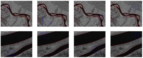
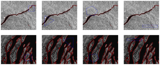
Figure 11.
Detected river channels in four SAR images of the SoDEF model with the diverse input level sets.
From Figure 11, we find that the SoDEF model created the same detected results with diverse input level sets. Therefore, its level set initialization is flexible. In other words, the SoDEF model is robust to the input level sets used.
5. Discussion
5.1. About Design and Contributions of the Proposed Model
The design of the proposed model mainly consisted of three parts: the SoDEF-fitting energy term, the adaptive AFCs, and the improved GDF. More specifically, we first defined a novel function by computing the sum of dual exponential functions, and used it to construct the data-fitting energy. Secondly, the adaptive AFCs were computed based on the mean and median AFCs. Thirdly, we substituted an edge indicator function for the Dirac function in the GDF. Therefore, the main contributions of our research are summarized as follows:
- (1)
- The defined SoDEF function was used to replace the quadratic function for constructing the data fitting energy, which provided much stronger energies and allowed the model to achieve the competence required to handle areas with close grayscales.
- (2)
- The adaptive AFCs were designed using two kinds of grayscale characteristics, and they were able to describe the region grayscale features more accurately and with better stability during the level set evolution, which created better detection performance.
- (3)
- We computed a LoG-based edge indicator, and used it to replace the Dirac function in the GDF, which encouraged the evolving level sets to stop at target edges. Thus, the efficiency of the proposed model was improved.
5.2. About Future Potential Impact and Weaknesses of the Proposed Model
We analyze the future potential impact from two aspects. In terms of methodology, the proposed model can be extended to multiple dimensions to achieve image multi-classification tasks. In addition, it can be regarded as an exploratory method in the evaluation and optimization of SAR-to-optical image translation. In terms of application, our proposed model succeeded in detecting river channels relatively accurately from SAR images, and this is conducive to flood disaster monitoring, map matching, etc.
Next, we also point out some weaknesses: (1) the complexity of the model implementation is still relatively high; (2) the proposed model only uses the global image features to guide the level sets. The above weaknesses limit the model’s detection efficiency.
6. Conclusions
In this research, a new level-set-based model guided by the SoDEF-fitting energies was developed to detect river channels in SAR images. Our model was constructed on the basis of three improvements, namely the SoDEF-fitting energy term, the adaptive AFCs, and the LoG-based edge indicator. Following this, corresponding river channel detection experiments were conducted on different types of real SAR images using the CV, CVGCO, RSFACI, JDF, RDE, WABSPF, FCAHS, AUMLSBM, and SoDEF methods. The experimental results imply that the SoDEF model outperforms the other experimental methods, and achieves more accurate and efficient river channel detection. More specifically, its detection QA are greater than 95 percent, and its detection QFA are smaller than 10 percent. Moreover, the input level sets of the SoDEF model can be set freely.
In addition, future research can be conducted in the following directions:
- (1)
- This model was implemented through level set evolution, which is not efficient enough. Its solving method needs to be optimized to reduce its implementation complexity.
- (2)
- The local image features can be added to the model’s data-fitting energy to further improve its river channel detection accuracy.
- (3)
- The multiple level sets were introduced to extend the proposed model to multiple dimensions, in order for it to be applied to image multi-classification.
Author Contributions
B.H. conceived the algorithm and designed the experiments; B.H. implemented the experiments and wrote the original manuscript; A.B. revised the manuscript. B.H. received the funding. All authors have read and agreed to the published version of the manuscript.
Funding
This research is supported by the National Natural Science Foundation of China under Grant 62201281, the Natural Science Foundation of Jiangsu Province under Grant BK20220392, and the Natural Science Research Start-up Foundation of Recruiting Talents of Nanjing University of Posts and Telecommunications under Grant NY222004.
Data Availability Statement
All data included in this study are available upon request by contact with the corresponding author.
Conflicts of Interest
We declare that there are no conflict.
Abbreviations
The following abbreviations are used in this manuscript:
| SAR | synthetic aperture radar |
| LSBM | level-set-based model |
| SoDEF | sum of dual exponential functions |
| AFCs | adaptive area-fitting centers |
| LCLSBMs | local characteristic-based LSBMs |
| GCLSBMs | global characteristic-based LSBMs |
| HCLSBMs | hybrid characteristic-LSBMs |
| ICV | inter-class variance |
| CV | Chan–Vese |
| CVGCO | coefficient of variation and graph-cut optimization |
| RSFACI | region-scalable fitting and atlas correcting information |
| AFT | atlas fitting term |
| MLRF | modified local region fitting |
| DWP | double-well potential |
| LGDF | local Gaussian distribution fitting |
| JDF | Jeffreys divergence fitting |
| RDE | reaction-diffusion energy |
| FCAHS | fuzzy clustering algorithm and hierarchical segmentation |
| OROEWA | optimized ratio of exponentially weighted averages |
| AUMLSBM | attention U-net and multi-scale LSBM |
| GDM | gradient descent method |
| GDF | gradient descent flow |
| DFE | data fitting energy |
References
- Dong, B.; Weng, G.; Jin, R. Active contour model driven by self organizing maps for image segmentation. Expert Syst. Appl. 2021, 177, 114948. [Google Scholar] [CrossRef]
- Bowden, A.; Sirakov, N.M. Active contour directed by the Poisson gradient vector field and edge tracking. J. Math. Imaging Vis. 2021, 63, 665–680. [Google Scholar] [CrossRef]
- Xu, H.; Lin, G. Incorporating global multiplicative decomposition and local statistical information for brain tissue segmentation and bias field estimation. Knowl. Based Syst. 2021, 223, 107070. [Google Scholar] [CrossRef]
- Fang, J.; Liu, H.; Zhang, L.; Liu, J.; Liu, H. Region-edge-based active contours driven by hybrid and local fuzzy region-based energy for image segmentation. Inf. Sci. 2021, 546, 397–419. [Google Scholar] [CrossRef]
- Liu, H.; Fang, J.; Zhang, Z.; Lin, Y. Localised edge-region-based active contour for medical image segmentation. IET Image Process. 2021, 15, 1567–1582. [Google Scholar] [CrossRef]
- Saman, S.; Narayanan, S.J. Active contour model driven by optimized energy functionals for MR brain tumor segmentation with intensity inhomogeneity correction. Multimed. Tools Appl. 2021, 80, 21925–21954. [Google Scholar] [CrossRef]
- Li, Y.; Cao, G.; Yu, Q.; Li, X. Active contours driven by non-local Gaussian distribution fitting energy for image segmentation. Appl. Intell. 2018, 48, 4855–4870. [Google Scholar] [CrossRef]
- Ali, H.; Rada, L.; Badshah, N. Image segmentation for intensity inhomogeneity in presence of high noise. IEEE Trans. Image Process. 2018, 27, 3729–3738. [Google Scholar] [CrossRef]
- Ren, S.; Wang, Y.; Dong, F. Piecewise constant level-set enhanced active shape reconstruction for electrical impedance tomography. Measurement 2021, 177, 109335. [Google Scholar] [CrossRef]
- Li, D.; Bei, L.; Bao, J.; Yuan, S.; Huang, K. Image contour detection based on improved level set in complex environment. Wirel. Netw. 2021, 27, 4389–4402. [Google Scholar] [CrossRef]
- Wang, G.; Dong, B. A new active contour model driven by pre-fitting bias field estimation and clustering technique for image segmentation. Eng. Appl. Artif. Intell. 2021, 104, 104299. [Google Scholar] [CrossRef]
- Rodtook, A.; Kirimasthong, K.; Lohitvisate, W.; Makhanov, S.S. Automatic initialization of active contours and level set method in ultrasound images of breast abnormalities. Pattern Recognit. 2018, 79, 172–182. [Google Scholar] [CrossRef]
- Sun, L.; Meng, X.; Xu, J.; Tian, Y. An image segmentation method using an active contour model based on improved SPF and LIF. Appl. Sci. 2018, 8, 2576. [Google Scholar] [CrossRef]
- Mahshid, F.; Kamran, K.; Sadegh, H.M.; Alireza, S. Morphological active contour driven by local and global intensity fitting for spinal cord segmentation from MR images. J. Neurosci. Methods 2018, 308, 116–128. [Google Scholar]
- Wan, M.; Gu, G.; Sun, J.; Qian, W.; Kan, R.; Qian, C.; Xavier, M. A level set method for infrared image segmentation using global and local information. Remote Sens. 2018, 10, 1039. [Google Scholar] [CrossRef]
- Han, B.; Wu, Y. Active contours driven by harmonic mean based KL divergence fitting energies for image segmentation. Electron. Lett. 2018, 54, 817–819. [Google Scholar] [CrossRef]
- Liu, S.; Peng, Y. A local region-based Chan-Vese model for image segmentation. Pattern Recognit. 2012, 45, 2769–2779. [Google Scholar] [CrossRef]
- Ali, H.; Badshah, N.; Chen, K.; Khan, G.A. A variational model with hybrid images data fitting energies for segmentation of images with intensity inhomogeneity. Pattern Recognit. 2016, 51, 27–42. [Google Scholar] [CrossRef]
- Birane, A.; Hamami, L. A fast level set image segmentation driven by a new region descriptor. IET Image Process. 2021, 15, 615–623. [Google Scholar] [CrossRef]
- Nithila, E.E.; Kumar, S.S. Segmentation of lung from CT using various active contour models. Biomed. Signal Process. Control 2019, 47, 57–62. [Google Scholar]
- Chan, T.F.; Vese, L.A. Active contours without edges. IEEE Trans. Image Process. 2001, 10, 266–277. [Google Scholar] [CrossRef]
- Subudhi, P.; Mukhopadhyay, S. A statistical active contour model for interactive clutter image segmentation using graph cut optimization. Signal Process. 2021, 184, 108056. [Google Scholar] [CrossRef]
- Ghosh, A.; Bandyopadhyay, S. Image co-segmentation using dual active contours. Appl. Soft. Comput. 2018, 66, 413–427. [Google Scholar] [CrossRef]
- Hussain, S.; Chun, Q.; Asif, M.R.; Khan, M.S. Active contours for image segmentation using complex domain-based approach. IET Image Process. 2016, 10, 121–129. [Google Scholar] [CrossRef]
- Lv, H.; Wang, Z.; Fu, S.; Zhang, C.; Liu, X. A robust active contour segmentation based on fractional-order differentiation and fuzzy energy. IEEE Access 2017, 5, 7753–7761. [Google Scholar] [CrossRef]
- Li, C.; Kao, C.; Gore, J.C.; Ding, Z. Minimization of region-scalable fitting energy for image segmentation. IEEE Trans. Image Process. 2008, 17, 1940–1949. [Google Scholar] [PubMed]
- Miao, J.; Huang, T.; Zhou, X.; Wang, Y.; Liu, J. Image segmentation based on an active contour model of partial image restoration with local cosine fitting energy. Inf. Sci. 2018, 447, 52–71. [Google Scholar] [CrossRef]
- Hai, M.; Wei, J.; Yang, Z.; Zuo, W.; Ling, H.; Luo, Y. LATE: A level-set method based on local approximation of Taylor expansion for segmenting intensity inhomogeneous images. IEEE Trans. Image Process. 2018, 27, 5016–5031. [Google Scholar]
- Yang, Y.; Wang, R.; Ren, H. Active contour model based on local intensity fitting and atlas correcting information for medical image segmentation. Multimed. Tools Appl. 2021, 80, 26493–26509. [Google Scholar] [CrossRef]
- Biswas, S.; Hazra, R. A level set model by regularizing local fitting energy and penalty energy term for image segmentation. Signal Process. 2021, 183, 108043. [Google Scholar] [CrossRef]
- Guo, B.; Cui, J.; Gao, B. Robust active contours based on local threshold preprocessing fitting energies for fast segmentation of inhomogenous images. Electron. Lett. 2021, 57, 576–578. [Google Scholar] [CrossRef]
- Mylona, E.A.; Savelonas, M.A.; Maroulis, D. Automated adjustment of region-based active contour parameters using local image geometry. IEEE Trans. Cybern. 2014, 44, 2757–2770. [Google Scholar] [CrossRef] [PubMed]
- Ozturk, N.; Ozturk, S. A new effective hybrid segmentation method based on C-V and LGDF. Signal Image Video Process. 2021, 15, 1313–1321. [Google Scholar] [CrossRef]
- Han, B.; Wu, Y. Active contour model for inhomogenous image segmentation based on Jeffreys divergence. Pattern Recognit. 2020, 107, 107520. [Google Scholar] [CrossRef]
- Zhang, L.; Peng, X.; Li, G.; Li, H. A novel active contour model for image segmentation using local and global region-based information. Mach. Vis. Appl. 2017, 28, 75–89. [Google Scholar] [CrossRef]
- Zhi, X.; Shen, H. Saliency driven region-edge-based top down level set evolution reveals the asynchronous focus in image segmentation. Pattern Recognit. 2018, 80, 241–255. [Google Scholar] [CrossRef]
- Safaie, A.H.; Rastiveis, H.; Shams, A.; Sarasua, W.A.; Li, J. Automated street tree inventory using mobile LiDAR point clouds based on Hough transform and active contours. ISPRS-J. Photogramm. Remote Sens. 2021, 174, 19–34. [Google Scholar]
- Wei, X.; Zheng, W.; Xi, C.; Shang, S. Shoreline extraction in SAR image based on advanced geometric active contour model. Remote Sens. 2021, 13, 642. [Google Scholar] [CrossRef]
- Li, Z.; Shi, W.; Myint, S.W.; Lu, P.; Wang, Q. Semi-automated landslide inventory mapping from bitemporal aerial photographs using change detection and level set method. Remote Sens. Environ. 2016, 175, 215–230. [Google Scholar] [CrossRef]
- Luo, S.; Sarabandi, K.; Tong, L.; Guo, S. An improved fuzzy region competition-based framework for the multiphase segmentation of SAR images. IEEE Trans. Geosci. Remote Sens. 2019, 58, 2457–2470. [Google Scholar] [CrossRef]
- Modava, M.; Akbarizadeh, G.; Soroosh, M. Integration of spectral histogram and level set for coastline detection in SAR Images. IEEE Trans. Aerosp. Electron. Syst. 2018, 55, 810–819. [Google Scholar] [CrossRef]
- Liu, J.; Wen, X.; Meng, Q.; Xu, H.; Yuan, L. Synthetic aperture radar image segmentation with reaction diffusion level set evolution equation in an active contour model. Remote Sens. 2018, 10, 906. [Google Scholar] [CrossRef]
- Han, B.; Wu, Y.; Basu, A. Adaptive active contour model based on weighted RBPF for SAR image segmentation. IEEE Access 2019, 7, 54522–54532. [Google Scholar] [CrossRef]
- Shang, R.; Chen, C.; Wang, G.; Jiao, L.; Okoth, M.A.; Stolkin, R. A thumbnail-based hierarchical fuzzy clustering algorithm for SAR image segmentation. Signal Process. 2020, 171, 107518. [Google Scholar] [CrossRef]
- Luo, R.; An, D.; Wang, W.; Huang, X. Improved ROEWA SAR image edge detector based on curvilinear structures extraction. IEEE Geosci. Remote Sens. Lett. 2020, 17, 631–635. [Google Scholar] [CrossRef]
- Xu, C.; Zhang, S.; Zhao, B.; Liu, C.; Sui, H.; Yang, W.; Mei, L. SAR image water extraction using the attention U-net and multi-scale level set method: Flood monitoring in South China in 2020 as a test case. Geo-Spat. Inf. Sci. 2022, 25, 209–223. [Google Scholar] [CrossRef]
- Wang, Y.; Huang, T.; Wang, H. Region-based active contours with cosine fitting energy for image segmentation. J. Opt. Soc. Am. A Opt. Image Sci. Vis. 2015, 32, 2237–2246. [Google Scholar] [CrossRef]
- Abdelsamea, M.M.; Tsaftaris, S.A. Active contour model driven by globally signed region pressure force. In Proceedings of the 18th International Conference on Digital Signal Processing, Fira, Greece, 5–7 July 2016; pp. 1–6. [Google Scholar]
Disclaimer/Publisher’s Note: The statements, opinions and data contained in all publications are solely those of the individual author(s) and contributor(s) and not of MDPI and/or the editor(s). MDPI and/or the editor(s) disclaim responsibility for any injury to people or property resulting from any ideas, methods, instructions or products referred to in the content. |
© 2023 by the authors. Licensee MDPI, Basel, Switzerland. This article is an open access article distributed under the terms and conditions of the Creative Commons Attribution (CC BY) license (https://creativecommons.org/licenses/by/4.0/).