Abstract
Hyperspectral images (HSI) have high-dimensional and complex spectral characteristics, with dozens or even hundreds of bands covering the same area of pixels. The rich information of the ground objects makes hyperspectral images widely used in satellite remote sensing. Due to the limitations of remote sensing satellite sensors, hyperspectral images suffer from insufficient spatial resolution. Therefore, utilizing software algorithms to improve the spatial resolution of hyperspectral images has become an urgent problem that needs to be solved. The spatial information and spectral information of hyperspectral images are strongly correlated. If only the spatial resolution is improved, it often damages the spectral information. Inspired by the high correlation between spectral information in adjacent spectral bands of hyperspectral images, a hybrid convolution and spectral symmetry preservation network has been proposed for hyperspectral super-resolution reconstruction. This includes a model to integrate information from neighboring spectral bands to supplement target band feature information. The proposed model introduces flexible spatial-spectral symmetric 3D convolution in the network structure to extract low-resolution and neighboring band features. At the same time, a combination of deformable convolution and attention mechanisms is used to extract information from low-resolution bands. Finally, multiple bands are fused in the reconstruction module, and the high-resolution hyperspectral image containing global information is obtained by Fourier transform upsampling. Experiments were conducted on the indoor hyperspectral image dataset CAVE, the airborne hyperspectral dataset Pavia Center, and Chikusei. In the X2 super-resolution task, the PSNR values achieved on the CAVE, Pavia Center, and Chikusei datasets were 46.335, 36.321, and 46.310, respectively. In the X4 super-resolution task, the PSNR values achieved on the CAVE, Pavia Center, and Chikusei datasets were 41.218, 30.377, and 38.365, respectively. The results show that our method outperforms many advanced algorithms in objective indicators such as PSNR and SSIM while maintaining the spectral characteristics of hyperspectral images.
1. Introduction
Hyperspectral image refers to an image with a continuous spectral range and containing multiple narrow-band wavebands. As a data cube, it contains hundreds of continuous spectral bands covering a wide range. For any point in space, a hyperspectral image can reconstruct the corresponding material area through its continuous and fine spectral curve and obtain its spatial and material properties. It is often used to obtain the spectral characteristics of surface materials, enabling quantitative analysis and the identification of material components. With the rapid development of aerospace and remote sensing technology, hyperspectral images based on remote sensing satellites are widely used in land detection [1,2], urban planning [3], road network layout [4], agricultural yield estimation [5], disaster prevention and control [6,7], and other fields.
Due to the unique imaging characteristics of hyperspectral images, spatial resolution and spectral resolution are two important criteria for measuring image quality in hyperspectral imaging systems. Spatial resolution refers to the smallest target size that can be resolved by the sensor, which can accurately describe the spatial information of image details. Spectral resolution refers to the resolution of feature detail information in the spectral dimension of an image, which can distinguish feature characteristics that are similar to the human eye and is widely used in remote sensing. In the imaging principle of hyperspectral images, each spectral image corresponds to a very narrow spectral window. Only by using a larger instantaneous field of view and a longer exposure time to collect enough photons can the signal-to-noise ratio of the spectral image be improved and a higher spatial resolution be obtained [8]. However, the spectral resolution is inversely proportional to the size of the instantaneous field of view. Therefore, a balance between spatial resolution and spectral resolution needs to be struck in the process of hyperspectral imaging. With the overlay of spectral features, hyperspectral images typically lower their spatial resolution to achieve higher spectral resolution [9]. If the emphasis is on hardware improvement, it not only poses challenges to current engineering technology but also goes against the lightweight and commercial design concept advocated by remote sensing satellites. Under the current limitations of hyperspectral imaging technology, it has become an urgent problem to maintain high spectral resolution while improving spatial resolution through software algorithms.
Image super-resolution reconstruction can infer a high-resolution image from one or multiple consecutive low-resolution images. It can break through the limitations of the imaging system and improve the spatial resolution of the image in the post-processing stage. The development of natural image super-resolution is becoming increasingly mature, while there is still much room for progress in hyperspectral image super-resolution. We classify them into three categories: single-frame HSI super-resolution methods; auxiliary image fusion hyperspectral image super-resolution (such as panchromatic, RGB, or multispectral image); and multi-frame fusion super-resolution methodd within hyperspectral images.
Single-frame hyperspectral image super-resolution methods are derived from natural image super-resolution methods, which mainly include interpolation-based methods, reconstruction-based methods, and learning-based methods. Among them, interpolation-based methods include nearest neighbor interpolation, first-order interpolation, bicubic interpolation, etc. However, interpolation methods can cause edge blur and artifacts and cannot fully utilize image abstraction information. Akgun et al. proposed a novel hyperspectral image acquisition model and a convex set projection algorithm to reconstruct high-resolution hyperspectral images [10]. Huang et al. proposed a dictionary-based super-resolution method by combining low-rank and group sparsity properties [11]. Wang et al. proposed a super-resolution method based on a non-local approximate tensor [12]. However, these methods require solving complex and time-consuming optimization problems during the testing phase and also require prior knowledge of the image, which makes it difficult to flexibly apply them to hyperspectral images. With the rapid development of convolutional neural networks, deep learning has shown superior performance in computer vision tasks. Super-resolution algorithms such as SRCNN [13], VDSR [14], EDSR [15], D-DPN [16], and SAN [17] have been proposed successively. They have shown superior performance in natural image super-resolution. However, when it comes to hyperspectral image super-resolution, the above-mentioned algorithms cannot explore spectral and spatial information, and their network representation ability is weak. Moreover, these natural image super-resolution methods have large parameters and are difficult to apply to multi-band hyperspectral images. In addition, there are few hyperspectral datasets available, which makes it difficult to support the learning of these algorithms. Yuan et al. proposed a method to transfer the knowledge learned from natural images to reconstruct high-resolution hyperspectral images [18]. However, the above method has limited improvement in spatial and spectral resolution.
The method of auxiliary image fusion hyperspectral image super-resolution combines low-resolution hyperspectral images with high-resolution RGB images, multispectral images, or panchromatic images. Starting from both spectral and spatial information, the method aims to obtain hyperspectral images with high spatial resolution and high spectral resolution. Which can be categorized into five types: pan-sharpening extension [19,20], Bayesian inference [21,22], matrix decomposition [23,24], tensor decomposition [25,26], and deep learning [27,28,29]. The above method requires high-resolution auxiliary images and has image registration issues, which make it difficult to implement in practical applications. The above method requires high-resolution auxiliary images and has image registration issues, which make it difficult to implement in practical applications.
In the absence of auxiliary images, the multi-frame fusion super-resolution method within a single hyperspectral image has received widespread attention. Jiang et al. [30] proposed a spatial-spectral prior network that utilizes the correlation between spatial and spectral information in hyperspectral images through group convolutions with progressive upsampling and shared parameters, but the network has a huge number of parameters. Wang et al. [31] proposed a sequential recursive feedback network that explores complementary and continuous information in hyperspectral images and preserves the spatial and spectral structures of spectral images. Hu et al. [32] proposed a hyperspectral image super-resolution method based on a deep information distillation network and internal fusion. Due to the strong correlation between bands in hyperspectral images, inspired by video multi-frame super-resolution, 3D convolution has begun to enter the field of hyperspectral image super-resolution [33]. Li et al. proposed a 2D and 3D hybrid module for image reconstruction, which to some extent alleviates the redundancy of the network structure while achieving the same performance [34]. To save parameters, Li et al. proposed a combined spectrum and feature context network [35]. In order to address the issue of excessive parameters in 3D convolutions, Jia et al. proposed a method called “Diffused Convolutional Neural Network for Hyperspectral Image Super-Resolution” [36], which has achieved good results.
It is difficult to simultaneously improve the spatial resolution of hyperspectral images while preserving their spectral characteristics. Hu et al. proposed a spectral difference network that separates spatial and spectral information for learning, which improves spatial resolution while preserving spectral characteristics [37]. However, the network structure is too redundant, and the improvement in spatial resolution is limited. Hu et al. [38] integrated the spectral difference module with the super-resolution reconstruction module, reducing the number of network parameters and enhancing the network’s generalization ability. References [39,40] propose a new method based on a spectral angle loss function to preserve spectral features.
In the problem of hyperspectral image super-resolution, traditional interpolation, Bayesian-based, matrix-based, and tensor decomposition methods require a significant amount of prior knowledge and have difficulties in model solving. Deep learning methods, relying on their excellent feature learning capabilities, construct models to obtain high-resolution images. However, current deep learning methods in hyperspectral super-resolution still have limitations, such as inadequate exploration of spectral and spatial correlations, redundant network structures, excessive parameters, and the inability to explore global features in both spatial and spectral domains. This paper proposes a hybrid convolution and spectral symmetry preservation network for hyperspectral super-resolution reconstruction. It uses a spatial-spectral symmetric 3D convolution to extract low-resolution bands and their adjacent band features, thus exploring the spatial and spectral correlation of hyperspectral images. A 2D convolution module, composed of deformable convolution and attention mechanisms, is designed to extract low-resolution band features and learn spatial information to the maximum extent. Finally, through the fusion module and Fourier transform reconstruction module, the network efficiently learns global and local information to obtain high-resolution hyperspectral images with high spectral fidelity.
Traditional algorithms for hyperspectral image super-resolution require a significant amount of prior knowledge and face challenges in the actual solving process. In contrast, deep-learning-based methods for hyperspectral image super-resolution have the ability to autonomously learn a large amount of feature information and construct high-resolution images. Therefore, this paper proposes a network framework based on deep learning. Compared to natural images, hyperspectral images have significantly more bands, and each band contains different spatial and spectral information. However, there is a high degree of similarity in the spectral information between adjacent bands. By effectively utilizing the spatial information between adjacent bands while preserving the spectral information of the current band, this paper proposes a design approach based on the supplementation of information from neighboring bands. The network consists of two parallel branches: a single-band feature extraction network and a multi-band feature extraction network. This network sequentially extracts the target super-resolution band and its adjacent bands. The target low-resolution band is processed by the single-band feature extraction network that consists of residual 2D convolutions, attention mechanisms, and deformable convolutions. The purpose of this network is to focus on the feature information of the target band. The residual 2D convolutions are used to extract both the shallow and deep information of the band. To capture more spatial and spectral information among different channels, we employ 3D residual convolutional modules in the multi-channel feature extraction network. Compared to 2D convolutions, 3D convolutions have an additional spatial dimension, making them widely used in hyperspectral image processing. However, the increased exploration capability in multiple dimensions also leads to an explosion of parameters. To address this issue, this paper introduces a novel spectral-symmetric 3D convolution, which significantly reduces the network parameters. In hyperspectral images, there exist distant spectral bands that contain similar spectral information and spatial information that can complement each other. To address this, we propose a context feature fusion module in our approach for integrating information from distant bands that mutually complement each other. Furthermore, in the reconstruction module, conventional upsampling methods often struggle to consider global information and only focus on the current pixel and its surrounding feature information. To overcome this limitation, we introduce Fourier transform upsampling in our approach for reconstructing high-resolution hyperspectral images. This approach takes into account global information and improves the overall quality of the reconstructed images.
2. Materials and Methods
2.1. Structure
The network structure of the hybrid convolution and spectral symmetry preservation network (HSSPN) is shown in Figure 1, which includes five parts: image input, feature extraction, feature fusion, image reconstruction, and image output. The network model is designed to improve the spatial resolution of the high-spectral image while maximizing the preservation of the spectral characteristics of the original high-spectral image. The spectral reflectance of adjacent spectral bands has high similarity, which represents similar spectral information between adjacent bands. While preserving the spectral information, fusing the spatial information of adjacent bands can effectively improve the spatial resolution of the low-resolution bands. Therefore, the input of the network consists of the low-resolution image LRt of the t-th band and the adjacent band images LRt+1 and LRt−1, as shown in Equation (1).
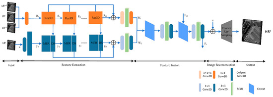
Figure 1.
Hybrid convolution and spectral symmetry preservation network (HSSPN).
When the first spectral band is selected, the adjacent bands are the second and third bands; when the last spectral band is selected, the adjacent bands are the second-to-last and third-to-last bands.
The feature extraction network structure uses two parallel networks, one for extracting multi-channel information and the other for extracting single-channel information. A shallow feature fusion module, denoted as DS, is added between the two parallel networks to fuse their features. To balance efficiency and performance, the multi-channel feature network uses the more flexible Res3D spatial-spectral symmetric 3D convolution module to extract multi-channel features, while the single-channel feature extraction network uses deformable convolution to extract shallow region features. Deep spatial features are extracted by mixed ECA attention mechanisms and a 2D residual convolution module (MER). The feature fusion network consists of two modules: the channel feature fusion module (CF) and the incremental feature fusion module (IF). The CF module fuses multi-channel features and single-channel features, while the IF module fuses incremental contextual spatial features. Both fusion modules deeply fuse spatial and spectral information between bands. To capture global information, the image reconstruction module uses Fourier transform upsampling and 2D convolution to reconstruct the image. The L1 loss combined with gradient loss (GV) is used as the loss function for the entire network.
2.2. Feature Extraction Module
The feature extraction process is mainly divided into two parallel networks: single-band feature extraction and multi-band feature extraction. At the same time, a shallow feature fusion module is added between the parallel networks.
2.2.1. Multi-Band Feature Extraction Network
The multi-channel feature extraction network is composed of several Res3D modules in series. Res3D is a residual network with spatially symmetric 3D convolution as its core. In this paper, 3D convolution is used to extract multi-channel features. Unlike 2D convolution, 3D convolution uses a three-dimensional convolution kernel to extract multi-dimensional information, which can analyze spatial dimension information and extract spectral dimension information at the same time. Three-dimensional convolution extracts features by sampling the input feature x with a 3D convolution kernel and weighting the sampled values with the function w, as shown in Equation (2) below when using a 3 × 3 × 3 convolution kernel:
where P0 represents the position of the output feature, and Pn and n represent the position and index of the 3 × 3 × 3 convolution kernel sampling grid. N represents the size of the sampling grid, and x represents the input multi-channel feature tensor It−1LR, ItLR, It+1LR.
Conventional 3D convolutions directly extracting model parameters result in a large number of parameters. Depthwise separable 3D convolutions were proposed to replace conventional 3D convolutions by modifying the filter k × k × k to k × 1 × 1 and 1 × k × k [41,42]. However, the model parameters are still too large and structurally redundant, which is not conducive to algorithm lightweighting. In this paper, spectral-symmetric 3D convolutions are used to extract multi-band features. Spectral-symmetric 3D convolutions perform one-dimensional convolutions along the three dimensions, decomposing the filter k × k × k into three dimensions of 1 × 1 × k, 1 × k × 1, and 1× 1 × k, simultaneously learning spectral and spatial features of multi-band images while saving a large number of network parameters. The calculation expression of the Res3D module is shown in Equation (3):
where YD represents the D-th function of the Res3D module, R0 represents the first input feature, and RD represents the output feature of the D-th Res3D module.
The Res3D module represents a residual network consisting of multiple 3D blocks, as shown in Figure 2. Each 3D block is connected to the next one through skip connections, allowing for maximum feature fusion and avoiding gradient explosion. Hyperspectral images contain rich information in three dimensions. To enhance the feature representation capability, inspired by [43], we design 3D blocks operating in different dimensions to extract features from multiple perspectives. Specifically, these blocks consist of three 1 × 1 × 1 convolutions at different scales with ReLU activation, enabling the extraction of diverse spatial and spectral features. Deep features are further extracted using 1 × 3 × 3 and 3 × 1 × 1 separable convolution kernels. The three layers of the network are interconnected with residual connections, maximizing feature integration and avoiding gradient explosion.
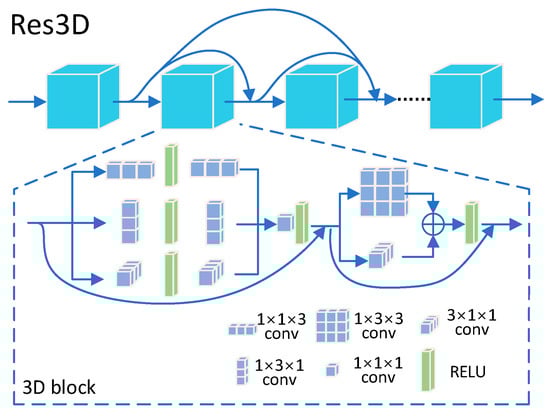
Figure 2.
Res3D network.
2.2.2. Single-Band Feature Extraction Network
To enhance the spatial resolution of hyperspectral images, this paper proposes a single-channel feature extraction network composed of deformable convolution modules and residual attention modules (MER).
The deformable convolution module consists of a 2D convolution and a deformable convolution. Compared to traditional convolution, it provides a more flexible receptive field and can extract the required target features to the maximum extent. The deformable convolution adds learnable offset values in the convolution kernel to extract actual object features more flexibly, as shown in Equation (4):
where P0 represents the location of the output features, Pn and n represent the 3 × 3 convolutional sampling grid, N represents the size of the sampling grid, and x represents the input multi-channel. The residual attention module (MER) is composed of the channel attention mechanism (ECA), residual 2D convolution, and shallow feature fusion module (DS), as shown in Figure 3.
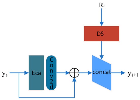
Figure 3.
Mixed ECA attention mechanisms and 2D residual convolution network.
ECA (efficient channel attention) is a lightweight channel attention mechanism that enhances information efficiency and effectiveness by incorporating local cross-channel interactions [44]. It automatically focuses on capturing detailed information across different channels within the network for hyperspectral super-resolution tasks. The specific steps of ECA can be summarized as follows: (1) The input feature tensor of size n × w × h is spatially downscaled by average pooling, resulting in global average values along the channel dimension. (2) One-dimensional convolution is applied to the global average values, generating a weight vector in the channel direction. (3) The weight vector is normalized using an activation function, yielding attention weights for each channel. (4) The attention weights are element-wise multiplied with the input feature tensor of size n × w × h, resulting in a weighted feature representation.
The feature tensor y with shape w × h × n obtained by the deformable convolution module is pooled with an average pooling operation. To ensure the attention mechanism is lightweight, a one-dimensional convolution with a kernel size of 1 is applied to the feature tensor, and then an activation function is used to obtain the weight values of each channel. The calculation is shown in Equation (5). The final output feature S is obtained by element-wise multiplication of the weight w with the corresponding weighted elements of the original input feature y. ECA enhances spatial feature extraction capabilities on a minimal parameter basis.
The output yd of the single-channel feature extraction network is calculated as shown in Equation (6). The shallow feature fusion module combines the multi-channel features extracted by Res3D with the single-channel features extracted by the residual attention module for shallow feature fusion. The shallow feature fusion network can preserve more edge and texture information, further improving the spatial resolution of the single channel.
where XD represents the function of the D-th MER module, y0 represents the first input feature after the calculation of deformable convolution, and yD represents the output feature of the D-th MER module.
2.2.3. Feature Fusion Network
The feature fusion module consists of two parts: the channel feature fusion module (CF) and the incremental feature fusion module (IF). The CF module fuses single-channel and multi-channel features, as shown in the following Equation (7).
where RD represents the features extracted by the multi-channel network and yD represents the features extracted by the single-channel network.
The incremental feature fusion module IF integrates the preserved features from the previous spectral band fusion network with the current spectral band fusion network, simplifying the network structure while exploring more spatial and spectral correlations. This is shown in detail in Figure 4.
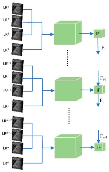
Figure 4.
Incremental feature fusion module network.
2.2.4. Image Reconstruction Network
Currently, image reconstruction usually employs spatial upsampling for multi-scale modeling, and interpolation, transpose convolution, and deconvolution operators are used in spatial upsampling. However, these operators heavily rely on local similarity features and cannot focus on global image information. According to the spectral convolution theorem, the Fourier domain follows global modeling, and it can focus more on global features. Therefore, in this paper, Fourier operators are used for image reconstruction.
The reconstruction module takes a low-resolution feature image X = RC×H×W as input and performs a Fourier transform (FFT) on the input-reconstructed feature image to obtain an amplitude variable A and a phase component P, as shown in Equations (8) and (9). Then, the two-dimensional H and W dimensions are padded twice periodically, as shown in Equation (10) and Figure 5. Finally, the padded A_pep and P_pep are input into two independent convolution modules with 1 × 1 kernels, and then an inverse Fourier transform (IFFT) is performed to project the padded A_pep and P_pep back into the spatial domain, resulting in a high-resolution image obtained through the periodic Fourier transform padding.
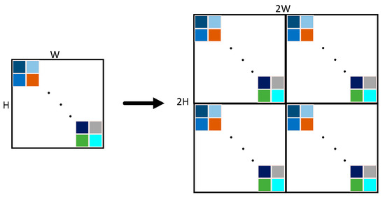
Figure 5.
Fourier transform upsampling.
2.2.5. Loss Function
This paper uses a loss function that combines L1 loss and gradient loss (GV) to guide the training of the network. The L1 loss calculates the absolute error between the target value and the estimated output value of the model, as shown in Equation (11).
The gradient variance loss measures the edge details of the image restoration by using the variance of the gradient map, calculated by the Sobel operator in the x and y directions of the high-resolution and low-resolution images. To better calculate the gradient variance, the image is segmented into n × n non-overlapping image blocks, and the average gradient value vi of each block is calculated along the y direction, as shown in Equation (12). Finally, the gradient variance loss (GV) is calculated by taking the mean of the gradients along the x and y directions of the high-resolution and low-resolution images, as shown in Equation (13). The overall loss is calculated as shown in Equation (14).
3. Results
3.1. Dataset and Parameter Settings
To evaluate the superiority of the method in this paper, experiments were conducted on the public hyperspectral datasets at CAVE, Pavia Center, and Chikusei. Relevant experiments were carried out.
The CAVE dataset is simulated by capturing images of materials and objects visible in the real world using a general-purpose calibrated pixel camera [45]. The spectral range of the images is from 400 nm to 700 nm, and the dataset size is 512 × 512 × 31. Six images are used as the test set, one image is used as the validation set, and the remaining 25 images are used as the training set.
The Pavia Center dataset is created using a reflective optics system imaging spectrometer (ROSIS) flown over Pavia in northern Italy. The wavelength range of the images is from 430 nm to 860 nm, and the original size of the dataset is 1096 × 1096. However, some samples do not contain any information, so the actual dataset size used is 1096 × 715 × 102. A 144 × 144 spectral image with the upper left corner as the origin is used as the test set, and a 144 × 144 image with the upper right corner as the origin is used as the validation set. The remaining data are used as the training set.
The Chikusei airborne hyperspectral dataset was captured by the Headwall Hyperspec-VNIR-C imaging sensor on 29 July 2014 in the agricultural and urban areas of Chikusei, Ibaraki, Japan [46]. The spectral range extends from 363 nm to 1018 nm, including 128 bands, and the scene consists of 2517 × 2335 pixels with a ground sampling distance of 2.5 m. The top left origin 1888 × 1888 is used as the training set, the top right origin 512 × 512 is used as the validation set, and the remaining part is used as the test set.
The acquisition of hyperspectral image data relies on expensive equipment and technical support, which also limits the accessibility of such data. Additionally, data collection is often constrained by factors such as the availability of specific geographic regions, limited time windows, or the presence of certain objects and scenes. Considering these factors, the availability of publicly accessible hyperspectral datasets is extremely limited. Therefore, due to the constraints of limited data, we applied data augmentation techniques to the training sets of the three publicly available hyperspectral datasets. The data augmentation methods primarily involved cropping, flipping at 90° and 180° angles, as well as scaling with factors of 1, 0.75, and 0.5.
3.2. Evaluation Accuracy
This paper mainly evaluates the performance differences between different methods from subjective and objective aspects. In order to conform to human subjective perception, we will show the comparison of the details of super-resolution reconstructed images between our method and other advanced algorithms. To quantitatively measure the effectiveness of our method, we use four evaluation methods, namely mean peak signal-to-noise ratio (MPSNR), structural similarity (SSIM) [47], and spectral angle mapper (SAM) [48]. The calculation formulas are shown in Equations (15)–(18).
3.3. Rigorousness Experiments and Parameter Settings
3.3.1. Component Analysis
In our network, modules such as Res3D, MER, deformable convolution, and Fourier-transform-based upsampling have demonstrated superior performance. We conducted extensive ablation experiments on both single-channel networks and the overall network to validate the effectiveness of the current combination in our network. Additionally, we present specific results of the X2 super-resolution task on the Pavia Center dataset, evaluating the performance using metrics such as PSNR (peak signal-to-noise ratio), SSIM (Structural Similarity Index), and SAM (spectral angle mapper).
Firstly, when performing hyperspectral image super-resolution using a single-channel network, we conducted related experiments on a 2DRes residual network alone, with the addition of deformable convolution, and with the inclusion of ECA channel attention. The results of these experiments are shown in Table 1. From the table, we can observe that the performance is poorest when using only the 2D residual network. The addition of deformable convolution improves the results by allowing the single-channel network to extract target features more flexibly, particularly enhancing the extraction of specific edges such as buildings and rivers. The combination of 2DRes and ECA channel attention performs better than the previous two approaches, as the channel attention maximizes the exploration of spectral features. However, it can be observed that when deformable convolution is introduced, the performance improves in terms of PSNR and SSIM values due to its focus on capturing deformable features and adaptively extracting relevant information. Compared to other combinations, the PSNR and SSIM values are higher. However, it is worth noting that the SAM (Spectral Angle Mapper) value, which represents the spectral characteristics, is larger in this case. Finally, the complete single-channel network achieves optimal performance.

Table 1.
Ablation study results on evaluating the efficiency of the MER.
Furthermore, we conducted related ablation experiments on the superior-performing single-channel network, multi-channel network, context feature fusion module IF, and Fourier-transform-based upsampling and reconstruction module in the overall network. The results of these experiments are shown in Table 2. When only MER or 3DRes is present in the network, the performance is poor. This is because when MER is used alone, it cannot fully utilize the information between spectral bands and can only focus on the current band’s information. Similarly, when Res3D is used alone, it fails to propagate shallow information to deeper layers. However, by incorporating feature fusion, combining the features of the single-channel and multi-channel networks, better results are obtained. The Fourier-transform-based upsampling module emphasizes global semantic information compared to traditional upsampling methods. Finally, when all the modules are combined, the overall network achieves the best performance.
Table 2.
Ablation study results on evaluating the efficiency of the network structure.
3.3.2. Research on Different Types of 3D Convolutions
In the Res3D network, different types of 3D convolutions have different parameters and feature extraction capabilities. Generally, 3D convolutions can be categorized as conventional 3D convolutions or separable 3D convolutions. In our Res3D network, we combine spectral symmetric 3D convolutions with separable 3D convolutions to achieve better performance while significantly reducing the number of network parameters, making the model more lightweight. We compared the results of using spectral symmetric 3D convolutions and other 3D convolutions for the X2 super-resolution task in the Pavia Center dataset, as shown in Table 3.
Table 3.
Performance of different types of 3D convolutions.
3.3.3. Parameter Settings
In the proposed HSSPN network, the number of MER and Res3D modules has an impact on the performance of our network. In this section, we discuss the influence of different numbers of MER and Res3D modules on the parameters and performance. The specific results can be seen in Table 4. Taking the Pavia Center dataset as an example for the X2 super-resolution task, we can observe that as the number of modules increases from 6 to 9, there is a noticeable improvement in metrics such as PSNR, SSIM, and SAM. However, from 9 to 10, the increase becomes minimal while the network parameters still significantly increase. Therefore, we set the number of MER and Res3D modules to 9.
Table 4.
Study investigating the influence of the number of MER and Res3D modules.
The network’s parameters include 2D convolution filters and are 64, and the ADAM optimizer (with β1 = 0.9 and β2 = 0.999) was used to optimize the designed model. The initial learning rate for all layers was set to 10−4, and it was halved every 35 epochs. All experiments were conducted on an Ubuntu 18.04 system, using an Intel(R) Xeon(R) Gold 6130 CPU and an NVIDIA GeForce GTX 3090 GPU with the PyTorch 1.80 deep learning framework.
3.4. Results and Analysis
In order to comprehensively evaluate the superiority of our method, this paper compares and analyzes it with current mainstream hyperspectral super-resolution algorithms, including Bicubic, VDSR, EDSR, MCNet, and SFCSR. The experimental results are analyzed from three datasets, CAVE, Pavia, and Chikusei, respectively.
3.4.1. CAVE
To visualize the face_ms test image in the CAVE dataset, the 26th, 17th, and 9th bands were used as RGB channels. As shown in Figure 6 for the 2x super-resolution comparison, respectively, it can be observed that the high-spectral reconstruction images obtained by Bicubic, VDSR, EDSR, MCNet, and SFCSR differ greatly from the original image, especially those obtained by Bicubic and VDSR. Moreover, due to the lack of learning between spectral features, the details of the images generated by EDSR are very blurry. Although MCNet and SFCSR utilize spectral features based on 2D/3D convolutions, there is still a slight spatial distortion in bright areas. From a visual perspective, the proposed method has better detail recovery than other methods. In terms of the evaluation metrics in Table 5, the proposed method outperforms other methods in terms of PSNR, SSIM, and SAM calculations.
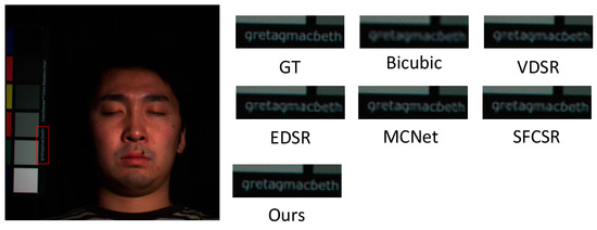
Figure 6.
The reconstructed images and detailed comparison images of the face_ms using various algorithms. Reconstructed images with spectral bands 26-17-9 as R-G-B channel with a scale factor of 2.
Table 5.
Quantitative evaluation on the CAVE dataset.
To further prove our advantage in spectral information reconstruction, we randomly selected the reflectance of pixels in different spectral bands from the face_ms image in Figure 7. It is clear that the spectral information generated by our method is closest to the HR image. The first few bands contain less bright information, and it is difficult to reflect the differences in algorithm performance. As the spectral wavelength increases, the accumulation of details in the bands gradually becomes prominent, and the differences in the detail reconstruction abilities of different algorithms become more pronounced. At the same time, due to the use of data normalization, the proposed method is also sensitive to the small features in the first few bands, which helps to reconstruct the overall detailed spectral characteristic curve of the HSI.
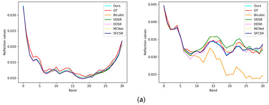
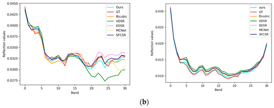
Figure 7.
Visual comparison of spectral distortion for face_ms image: (a) pixel position (220, 20), (339, 439) on the CAVE dataset with a scale factor of 2; (b) pixel position (250, 20), (293, 499) on the CAVE dataset with a scale factor of 4.
3.4.2. Pavia Center
In the Pavia dataset, the 13th, 35th, and 60th spectral bands were used to synthesize a false-color image, and Figure 8 shows the details of the RGB images restored by all methods at a upsampling ratio of 2. From the figure, it can be seen that most methods, such as Bicubic, EDSR, and VDSR, cannot reconstruct the details of the roof stripes well. The roof stripes generated by MCNet and SFCSR are relatively blurry, and some tile details are missing, so they cannot reconstruct the real roof details. Our proposed method can effectively reconstruct the contour details in detail. The quantitative analysis results are shown in Table 6. From the perspective of spatial information reconstruction and spectral information distortion reduction, our proposed method is significantly better than other methods. It can be seen from the experimental results and analysis that our proposed method demonstrates superior performance. The spectral reconstructed reflection curves of quadruple and double hyper-segmented random pixel points on the Pavia center data are also shown in Figure 9.
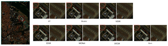
Figure 8.
The reconstructed images and detailed comparison images of the Pavia using various algorithms. Reconstructed images with spectral bands 60-35-13 as R-G-B channel with a scale factor of 2.
Table 6.
Quantitative evaluation on the Pavia.
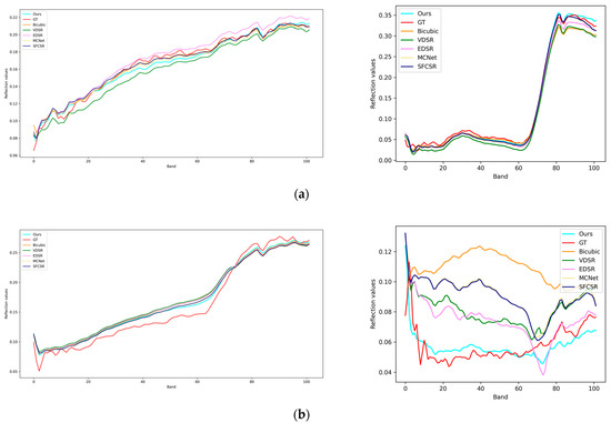
Figure 9.
Visual comparison of spectral distortion for Pavia center image: (a) pixel position (482, 433), (452, 344) on the Pavia center dataset with a scale factor of 2; (b) pixel position (583, 413), (337, 424) on the Pavia center dataset with a scale factor of 4.
3.4.3. Chikusei
In the Chikusei dataset, the 70th, 100th, and 36th spectral bands were used to synthesize a false-color image, and Figure 10 shows the details of the RGB images restored by all methods at a upsampling ratio of 2. From Figure 10, it can be seen that the bicubic method results in overly smooth road details and a loss of edge information due to its smooth interpolation. VDSR learns more features through a residual network, but its network structure is simple and limited in terms of learning feature content. The Chikusei dataset mainly contains outdoor land area information, and the difference in information between multiple bands is small. Therefore, compared to MXNet and SFCSR, which use 3D convolution, EDSR performs better on this dataset. In addition to using 3D convolution, the reconstruction module of our proposed method also relies on Fourier transform upsampling to explore global information, which is superior to EDSR in restoring road details. Specific objective evaluation indicators can be seen in Table 7, where EDSR performs best compared to our proposed method. Our proposed method outperforms EDSR and SFCSR in PSNR, SSIM, and SAM indicators. When the upsampling ratio is 2, compared to EDSR, PSNR improves by 0.198, SSIM improves by 0.0004, and SAM decreases by 0.020; when the upsampling ratio is 4, PSNR improves by 0.050, and SSIM improves by 0.0039. To demonstrate the superiority of our proposed method in spectral preservation, we randomly selected two pixels in the images that were magnified 2 and 4 times, respectively, and plotted their spectral reflectance curves. The results are shown in Figure 11. It can be clearly seen that the spectral reflectance of our proposed method is closer to that of the real image.
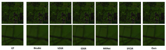
Figure 10.
The reconstructed images and detailed comparison images of the Pavia using various algorithms. Reconstructed images with spectral bands 70-100-30 as R-G-B channel with a scale factor of 2.
Table 7.
Quantitative evaluation on the Chikusei.
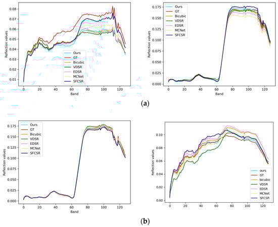
Figure 11.
Visual comparison of spectral distortion for Chikusei image: (a) pixel position (2248, 2093), (2037, 2124) on the Chikusei dataset with a scale factor of 2; (b) pixel position (1922, 2013), (1897, 1924) on the Chikusei dataset with a scale factor of 4.
4. Conclusions
In this paper, a hybrid convolution and spectral symmetry preservation network is presented. Observation has demonstrated that hybrid convolution had excellent performance on the spatial information of hyperspectral images; in this way, mixed 3D convolution and 2D convolution enable hierarchical extraction of spatial information and spectral information. The entire network can be divided into five modules: image input, feature extraction, feature fusion, image reconstruction, and image output. Feature extraction is divided into two parallel networks: single-channel feature extraction and multi-channel feature extraction to extract spatial and spectral information at multiple scales. Feature fusion proposes a multi-band fusion method and a contextual feature incremental fusion module to simplify the information redundancy in hyper-resolution networks of hyperspectral images while exploring more spectral information. Image reconstruction explores global image information through Fourier transform upsampling. Experimental results and data analysis on three datasets, which were captured by different sensors, have demonstrated the effectiveness of the proposed method. However, the method presented in this paper still suffers from excessive model parameters and a relatively redundant model structure, indicating the need for further optimization.
Author Contributions
Conceptualization, L.B. and D.D.; methodology, L.B.; software, D.D.; validation, L.B., D.D. and Z.Z.; formal analysis, D.D.; investigation, L.B.; resources, L.B.; data curation, D.D.; writing—original draft preparation, D.D.; writing—review and editing, L.B., D.D. and M.D.; visualization, L.B., D.D. and Z.Z.; supervision, M.D.; project administration, L.B. and M.D.; funding acquisition, L.B., Y.Y. and Z.Z.; All authors have read and agreed to the published version of the manuscript.
Funding
This research was funded by the National Key R&D Program of China (grant number 2020YFA0713503), the Science and Technology Project of Hunan Provincial Natural Resources Department (grant number 2022JJ30561), the Scientific Research Project of Natural Resources in Hunan Province (grant number 2022-15), and the Science and Technology Project of Hunan Provincial Natural Resources Department (grant number 2023JJ30582) and supported by Postgraduate Scientific Research Innovation Project of Hunan Province (grant number QL20220161) and Postgraduate Scientific Research Innovation Project of Xiang-tan University (grant number XDCX2022L024). All authors have read and agreed to the published version of the manuscript.
Data Availability Statement
The data and the details regarding the data supporting the reported results in this paper are available from the corresponding author.
Acknowledgments
The authors would like to take this opportunity to thank the editors and the reviewers for their detailed comments and suggestions.
Conflicts of Interest
The authors declare no conflict of interest.
References
- Jalal, R.; Iqbal, Z.; Henry, M.; Franceschini, G.; Islam, M.S.; Akhter, M.; Khan, Z.T.; Hadi, M.A.; Hossain, M.A.; Mahboob, M.G.; et al. Toward Efficient Land Cover Mapping: An Overview of the National Land Representation System and Land Cover Map 2015 of Bangladesh. IEEE J. Sel. Top. Appl. Earth Obs. Remote Sens. 2019, 12, 3852–3861. [Google Scholar] [CrossRef]
- Zhang, P.; Wang, N.; Zheng, Z.; Xia, J.; Zhang, L.; Zhang, X.; Zhu, M.; He, Y.; Jiang, L.; Zhou, G.; et al. Monitoring of Drought Change in the Middle Reach of Yangtze River. In Proceedings of the IGARSS 2018—2018 IEEE International Geoscience and Remote Sensing Symposium, Valencia, Spain, 22–27 July 2018; pp. 4935–4938. [Google Scholar] [CrossRef]
- Goetzke, R.; Braun, M.; Thamm, H.P.; Menz, G. Monitoring and modeling urban land-use change with multitemporal satellitedata. In Proceedings of the IGARSS 2008—2008 IEEE International Geoscience and Remote Sensing Symposium, Boston, MA, USA, 7–11 July 2008; Volume 4, pp. 510–513. [Google Scholar]
- Darweesh, M.; Mansoori, S.A.; Alahmad, H. Simple Roads Extraction Algorithm Based on Edge Detection Using Satellite Images. In Proceedings of the 2019 IEEE 4th International Conference on Image, Vision and Computing, ICIVC, Xiamen, China, 5–7 July 2019; pp. 578–582. [Google Scholar] [CrossRef]
- Kussul, N.; Shelestov, A.; Yailymova, H.; Yailymov, B.; Lavreniuk, M.; Ilyashenko, M. Satellite Agricultural Monitoring in Ukraineat Country Level: World Bank Project. In Proceedings of the 2020 IEEE International Geoscience and Remote Sensing Symposium, Waikoloa, HI, USA, 26 September–2 October 2020; pp. 1050–1053. [Google Scholar] [CrossRef]
- Di, Y.; Xu, X.; Zhang, G. Research on secondary analysis method of synchronous satellite monitoring data of power grid wildfire. In Proceedings of the 2020 IEEE International Conference on Information Technology, Big Data and Artificial Intelligence, ICIBA, Chongqing, China, 6–8 November 2020; pp. 706–710. [Google Scholar] [CrossRef]
- Chen, M.; Duan, Z.; Lan, Z.; Yi, S. Scene Reconstruction Algorithm for Unstructured Weak-Texture Regions Based on Stereo Vision. Appl. Sci. 2023, 13, 6407. [Google Scholar] [CrossRef]
- Liu, Y.N. Development of hyperspectral imaging remote sensing technology. Natl. Remote Sens. Bull. 2021, 25, 439–459. [Google Scholar] [CrossRef]
- Liu, H.; Gu, Y.; Wang, T.; Li, S. Satellite Video Super-Resolution Based on Adaptively Spatiotemporal Neighbors and Nonlocal Similarity Regularization. IEEE Trans. Geosci. Remote Sens. 2020, 58, 8372–8383. [Google Scholar] [CrossRef]
- Akgun, T.; Altunbasak, Y.; Mersereau, R. Super-resolution reconstruction of hyperspectral images. IEEE Trans. Image Process. 2005, 14, 1860–1875. [Google Scholar] [CrossRef] [PubMed]
- Huang, H.; Yu, J.; Sun, W. Super-resolution mapping via multi-dictionary based sparse representation. In Proceedings of the 2014 IEEE InternationalConference on Acoustics, Speech and Signal Processing (ICASSP), Florence, Italy, 4–9 May 2014; pp. 3523–3527. [Google Scholar] [CrossRef]
- Wang, Y.; Chen, X.; Han, Z.; He, S. Hyperspectral Image Super-Resolution via Nonlocal Low-Rank Tensor Approximation and Total Variation Regularization. Remote Sens. 2017, 9, 1286. [Google Scholar] [CrossRef]
- Dong, C.; Loy, C.C.; He, K.; Tang, X. Image Super-Resolution Using Deep Convolutional Networks. IEEE Trans. Pattern Anal. Mach. Intell. 2016, 38, 295–307. [Google Scholar] [CrossRef]
- Kim, J.; Lee, J.K.; Lee, K.M. Accurate image super-resolution using very deep convolutional networks. In Proceedings of the IEEE Conference on Computer Vision and Pattern Recognition, Las Vegas, NV, USA, 27–30 June 2016; pp. 1646–1654. [Google Scholar]
- Lim, B.; Son, S.; Kim, H.; Nah, S.; Lee, K.M. Enhanced deep residual networks for single image super-resolution. In Proceedings of the IEEE Conference on Computer Vision and Pattern Recognition Workshops (CVPRW), Honolulu, HI, USA, 12–26 July 2017; pp. 1132–1140. [Google Scholar] [CrossRef]
- Haris, M.; Shakhnarovich, G.; Ukita, N. Deep Back-Projection Networks for Super-Resolution. In Proceedings of the 2018 IEEE/CVF Conference on Computer Vision and Pattern Recognition, Salt Lake City, UT, USA, 18–23 June 2018; pp. 1664–1673. [Google Scholar] [CrossRef]
- Dai, T.; Cai, J.; Zhang, Y.; Xia, S.-T.; Zhang, L. Second-Order Attention Network for Single Image Super-Resolution. In Proceedings of the IEEE Computer Society Conference on Computer Vision and Pattern Recognition, Long Beach, CA, USA, 15–20 June 2019; pp. 11057–11066. [Google Scholar] [CrossRef]
- Yuan, Y.; Zheng, X.; Lu, X. Hyperspectral Image Superresolution by Transfer Learning. IEEE J. Sel. Top. Appl. Earth Obs. Remote Sens. 2017, 10, 1963–1974. [Google Scholar] [CrossRef]
- Gomez, R.B.; Jazaeri, A.; Kafatos, M. Wavelet-based hyperspectral and multispectral image fusion. In Geo-Spatial Image and Data Exploitation II; SPIE: Bellingham, WA, USA, 2001; pp. 36–42. [Google Scholar] [CrossRef]
- Aiazzi, B.; Baronti, S.; Selva, M. Improving Component Substitution Pansharpening Through Multivariate Regression of MS ++Pan Data. IEEE Trans. Geosci. Remote Sens. 2007, 45, 3230–3239. [Google Scholar] [CrossRef]
- Wei, Q.; Bioucas-Dias, J.; Dobigeon, N.; Tourneret, J.-Y. Hyperspectral and Multispectral Image Fusion Based on a Sparse Representation. IEEE Trans. Geosci. Remote Sens. 2015, 53, 3658–3668. [Google Scholar] [CrossRef]
- Akhtar, N.; Shafait, F.; Mian, A. Bayesian sparse representation for hyperspectral image super resolution. In Proceedings of the 2015 IEEE Conference on Computer Vision and Pattern Recognition (CVPR), Boston, MA, USA, 7–12 June 2015; pp. 3631–3640. [Google Scholar] [CrossRef]
- Yokoya, N.; Yairi, T.; Iwasaki, A. Coupled Nonnegative Matrix Factorization Unmixing for Hyperspectral and Multispectral Data Fusion. IEEE Trans. Geosci. Remote Sens. 2011, 50, 528–537. [Google Scholar] [CrossRef]
- Liu, J.; Wu, Z.; Xiao, L.; Sun, J.; Yan, H. A Truncated Matrix Decomposition for Hyperspectral Image Super-Resolution. IEEE Trans. Image Process 2020, 29, 8028–8042. [Google Scholar] [CrossRef]
- Li, S.; Dian, R.; Fang, L.; Bioucas-Dias, J.M. Fusing Hyperspectral and Multispectral Images via Coupled Sparse Tensor Factorization. IEEE Trans. Image Process 2018, 27, 4118–4130. [Google Scholar] [CrossRef]
- Xu, Y.; Wu, Z.; Chanussot, J.; Wei, Z. Nonlocal Patch Tensor Sparse Representation for Hyperspectral Image Super-Resolution. IEEE Trans. Image Process 2019, 28, 3034–3047. [Google Scholar] [CrossRef] [PubMed]
- Palsson, F.; Sveinsson, J.R.; Ulfarsson, M.O. Multispectral and Hyperspectral Image Fusion Using a 3-D-Convolutional Neural Network. IEEE Geosci. Remote Sens. Lett. 2017, 14, 639–643. [Google Scholar] [CrossRef]
- Qu, Y.; Qi, H.; Kwan, C. Unsupervised Sparse Dirichlet-Net for Hyperspectral Image Super-Resolution. In Proceedings of the 2018 IEEE/CVF Conference on Computer Vision and Pattern Recognition, Salt Lake City, UT, USA, 18–23 June 2018; pp. 2511–2520. [Google Scholar] [CrossRef]
- Zheng, K.; Gao, L.; Liao, W.; Hong, D.; Zhang, B.; Cui, X.; Chanussot, J. Coupled Convolutional Neural Network with Adaptive Response Function Learning for Unsupervised Hyperspectral Super Resolution. IEEE Trans. Geosci. Remote Sens. 2020, 59, 2487–2502. [Google Scholar] [CrossRef]
- Jiang, J.; Sun, H.; Liu, X.; Ma, J. Learning Spatial-Spectral Prior for Super-Resolution of Hyperspectral Imagery. IEEE Trans. Comput. Imaging 2020, 6, 1082–1096. [Google Scholar] [CrossRef]
- Wang, X.; Ma, J.; Jiang, J. Hyperspectral Image Super-Resolution via Recurrent Feedback Embedding and Spatial–Spectral Consistency Regularization. IEEE Trans. Geosci. Remote Sens. 2022, 60, 5503113. [Google Scholar] [CrossRef]
- Hu, J.; Zhao, M.; Li, Y. Hyperspectral Image Super-Resolution by Deep Spatial-Spectral Exploitation. Remote Sens. 2019, 11, 1229. [Google Scholar] [CrossRef]
- Mei, S.; Yuan, X.; Ji, J.; Zhang, Y.; Wan, S.; Du, Q. Hyperspectral Image Spatial Super-Resolution via 3D Full Convolutional Neural Network. Remote Sens. 2017, 9, 1139. [Google Scholar] [CrossRef]
- Li, Q.; Wang, Q.; Li, X. Mixed 2D/3D Convolutional Network for Hyperspectral Image Super-Resolution. Remote Sens. 2020, 12, 1660. [Google Scholar] [CrossRef]
- Wang, Q.; Li, Q.; Li, X. Hyperspectral Image Superresolution Using Spectrum and Feature Context. IEEE Trans. Ind. Electron. 2021, 68, 11276–11285. [Google Scholar] [CrossRef]
- Jia, S.; Zhu, S.; Wang, Z.; Xu, M.; Wang, W.; Guo, Y. Diffused Convolutional Neural Network for Hyperspectral Image Super-Resolution. IEEE Trans. Geosci. Remote Sens. 2023, 61, 5504615. [Google Scholar] [CrossRef]
- Hu, J.; Li, Y.; Xie, W. Hyperspectral Image Super-Resolution by Spectral Difference Learning and Spatial Error Correction. IEEE Geosci. Remote Sens. Lett. 2017, 14, 1825–1829. [Google Scholar] [CrossRef]
- Hu, J.; Jia, X.; Li, Y.; He, G.; Zhao, M. Hyperspectral Image Super-Resolution via Intrafusion Network. IEEE Trans. Geosci. Remote Sens. 2020, 58, 7459–7471. [Google Scholar] [CrossRef]
- Li, Y.; Zhang, L.; Dingl, C.; Wei, W.; Zhang, Y. Single Hyperspectral Image Super-Resolution with Grouped Deep Recursive Residual Network. In Proceedings of the 2018 IEEE Fourth International Conference on Multimedia Big Data (BigMM), Xi’an, China, 13–16 September 2018; pp. 1–4. [Google Scholar] [CrossRef]
- Lu, X.; Liu, X.; Zhang, L.; Jia, F.; Yang, Y. Hyperspectral image super-resolution based on attention ConvBiLSTM network. Int. J. Remote Sens. 2022, 43, 5059–5074. [Google Scholar] [CrossRef]
- Hu, Z.; Hu, Y.; Liu, J.; Wu, B.; Han, D.; Kurfess, T. 3D separable convolutional neural network for dynamic hand gesture recognition. Neurocomputing 2018, 318, 151–161. [Google Scholar] [CrossRef]
- Qiu, Z.; Yao, T.; Mei, T. Learning spatio-temporal representationwith pseudo-3D residual networks. In Proceedings of the IEEE International Conference on Computer Vision (ICCV), Venice, Italy, 22–29 October 2017; pp. 5533–5541. [Google Scholar]
- Hou, J.; Zhu, Z.; Hou, J.; Liu, H.; Zeng, H.; Meng, D. Deep Diversity-Enhanced Feature Representation of Hyperspectral Images. arXiv preprint 2023, arXiv:2301.06132. [Google Scholar]
- Wang, Q.; Wu, B.; Zhu, P.; Li, P.; Zuo, W.; Hu, Q. ECA-Net: Efficient Channel Attention for Deep Convolutional Neural Networks. In Proceedings of the 2020 IEEE/CVF Conference on Computer Vision and Pattern Recognition (CVPR), Seattle, WA, USA, 14–19 June 2020; pp. 11531–11539. [Google Scholar] [CrossRef]
- Yasuma, F.; Mitsunaga, T.; Iso, D.; Nayar, S.K. Generalized Assorted Pixel Camera: Postcapture Control of Resolution, Dynamic Range, and Spectrum. IEEE Trans. Image Process 2010, 19, 2241–2253. [Google Scholar] [CrossRef]
- Yokoya, N.; Iwasaki, A. Airborne Hyperspectral Data Over Chikusei; University of Tokyo: Tokyo, Japan, 2016. [Google Scholar]
- Wang, Z.; Bovik, A.C.; Sheikh, H.R.; Simoncelli, E.P. Image Quality Assessment: From Error Visibility to Structural Similarity. IEEE Trans. Image Process. 2004, 13, 600–612. [Google Scholar] [CrossRef]
- Yuhas, R.; Goetz, A.F.H.; Boardman, J.W. Discrimination among semi-arid landscape endmembers using the spectral angle mapper (SAM) algorithm. In Proceedings of the JPL, Summaries of the Third Annual JPL Airborne Geoscience Workshop; 1–5 June 1992, NASA: Washington, DC, USA, 1992; Volume 1, pp. 147–149. [Google Scholar]


Disclaimer/Publisher’s Note: The statements, opinions and data contained in all publications are solely those of the individual author(s) and contributor(s) and not of MDPI and/or the editor(s). MDPI and/or the editor(s) disclaim responsibility for any injury to people or property resulting from any ideas, methods, instructions or products referred to in the content. |
© 2023 by the authors. Licensee MDPI, Basel, Switzerland. This article is an open access article distributed under the terms and conditions of the Creative Commons Attribution (CC BY) license (https://creativecommons.org/licenses/by/4.0/).