Technical Note

TRP-Oriented Hyperspectral Remote Sensing Image Classification Using Entropy-Weighted Ensemble Algorithm

The Institute for Remote Sensing Science and Application, School of Geomatics, Liaoning Technical University, Fuxin 123000, China
*
Author to whom correspondence should be addressed.
Remote Sens. 2023, 15(9), 2315; https://doi.org/10.3390/rs15092315
Submission received: 17 March 2023 / Revised: 23 April 2023 / Accepted: 26 April 2023 / Published: 27 April 2023
(This article belongs to the Special Issue Hyperspectral Remote Sensing Imaging and Processing)

Abstract

:
The problem that the randomly generated random projection matrix will lead to unstable classification results is addressed in this paper. To this end, a Tighter Random Projection-oriented entropy-weighted ensemble algorithm is proposed for classifying hyperspectral remote sensing images. In particular, this paper presents a random projection matrix selection strategy based on the separable information of a single class able to project the features of a certain class of objects. The projection result is measured by the degree of separability, thereby obtaining the low-dimensional image with optimal separability of the class. After projecting samples with the same random projection matrix, to calculate the distance matrix, the Minimum Distance classifier is devised, repeating for all classes. Finally, the weight of the distance matrix is considered in ensemble classification by using the information entropy. The proposed algorithm is tested on real hyperspectral remote sensing images. The experiments show an increase in both stability and performance.

1. Introduction

With the continuous improvement of sensor technology, the spectral resolution of remote sensing images is getting higher and higher, usually including dozens to hundreds of bands [1,2]. Hyperspectral remote sensing image classification is essentially the process of dividing the image domains into non-overlapping sub-regions according to the feature information of the images and assigning a specific class to each sub-region [3,4]. While providing rich spectral information, it also greatly increases the computational cost required for hyperspectral remote sensing image classification. Therefore, dimensionality reduction is usually required before classification [5,6,7].
Traditional dimensionality reduction methods can be roughly divided into two types: band selection [8,9,10] and feature extraction based on data transformation [11,12,13]. The first type of method is generally based on a certain evaluation criterion function to perform a band combination search to achieve the purpose of dimensionality reduction. The second type of method is to map hyperspectral remote sensing images to a low-dimensional space through linear or nonlinear transformation, thereby obtaining a low-dimensional representation of the original data set. For low-configuration hardware, these methods cannot reduce the dimensionality in an acceptable timeframe, which greatly limits the application of hyperspectral remote sensing images [14,15]. Random Projection (RP) has the characteristics of being independent of high-dimensional data and simple to calculate, which is a dimensionality reduction algorithm with little information loss [16,17]. This algorithm provides a feasible mapping way for the Johnson-Lindenstrauss lemma [18,19], which has been widely used in biology, environmental monitoring, and disaster monitoring fields [20,21,22].
The classification task has attracted many researchers to conduct research in this field, and many algorithms of dimensionality reduction and classification have been proposed [23,24,25]. According to the conditions of prior information, it can be divided into supervised classification algorithms and unsupervised classification algorithms. Representative supervised classification algorithms include Minimum Distance (MD), Support Vector Machines (SVM), and Convolutional Neural Networks [26,27,28]. Zhou et al. [29] proposed a radical algorithm through a self-organizing pixel entanglement neural network. This network used pixel entanglement coefficient to mine the quantum entanglement relationship on the array space. Zheng et al. [30] proposed a spectrum interference-based two-level data augmentation method in deep learning for automatic modulation classification. This algorithm is the first time radio signals were used to help modulation classification by considering the frequency domain information. Zhao et al. [31] proposed a Tighter RP based on Minimum Intra-class Variance (TRP-MIV) algorithm for hyperspectral remote sensing image classification. This algorithm selects the random projection matrix to generate low-dimensional images and uses the MD classifier [32] for subsequent classification. Zhao and Mao [33] proposed a semi-random projection method, which uses Linear Discriminant Analysis (LDA) to calculate each column vector in the projection matrix and calculates the projection matrix by repeating it multiple times. Fuzzy C-Means (FCM) clustering algorithm is one of the representative unsupervised classification algorithms [34]. Fowler et al. [35] proposed a Compressive-Projection Principal Component Analysis (CPPCA) algorithm for hyperspectral images. The CPPCA algorithm first uses the RP algorithm to project the hyperspectral images into the low-dimensional space to reduce the computational complexity of image processing. Next, Principal Component Analysis (PCA) is used to further process the dimensionality reduction results of the RP algorithm in the projection direction with the smallest mean square error. Finally, the final low-dimensional image is obtained. Pasunuri et al. [36] combined the PCA, RP, and K-means algorithms to classify the high-dimensional data. Alshamiri et al. [37] proposed a classification algorithm combining Extreme Learning Machine (ELM) and RP, which uses ELM to transform high-dimensional data and keeps the linear class separability of high-dimensional data in the ELM feature space. The RP is used to project the transformation result of ELM into a low-dimensional space. Rathore et al. [38] proposed a new Cumulative Agreement Fuzzy C-Means (CAFCM) algorithm, which uses the clustering effectiveness index to sort all the membership matrices and accumulates all the membership matrices to get the final similarity measure matrix. Anderlucci et al. [39] proposed a model-based clustering algorithm for high-dimensional data, which obtains the final segmentation result through consensus aggregation. Although the RP algorithm can achieve simple and fast dimensionality reduction results, since the random projection matrix is randomly generated, it may generate low-dimensional images that are not conducive to subsequent classification tasks and have the disadvantage of high randomness.
To solve the above problems, this paper exploits TRP-oriented hyperspectral remote sensing image classification using an entropy-weighted ensemble algorithm. The proposed algorithm can effectively improve the classification accuracy of hyperspectral remote sensing images. First, based on the TRP algorithm, a distance matrix suitable for a certain class is generated by combining the random projection matrix selection strategy based on the separable information of a single class and the MD classifier. The above steps are repeated for all classes and the information entropy of the distance matrix of all classes is calculated as weights to generate the final similarity measure matrix, thereby realizing the classification of hyperspectral remote sensing images. The structure of this paper is organized as below. Section 2 and Section 3 give the materials and the proposed algorithm, respectively. The results and discussion are provided in Section 4. Finally, this paper is concluded in Section 5.

2. Materials

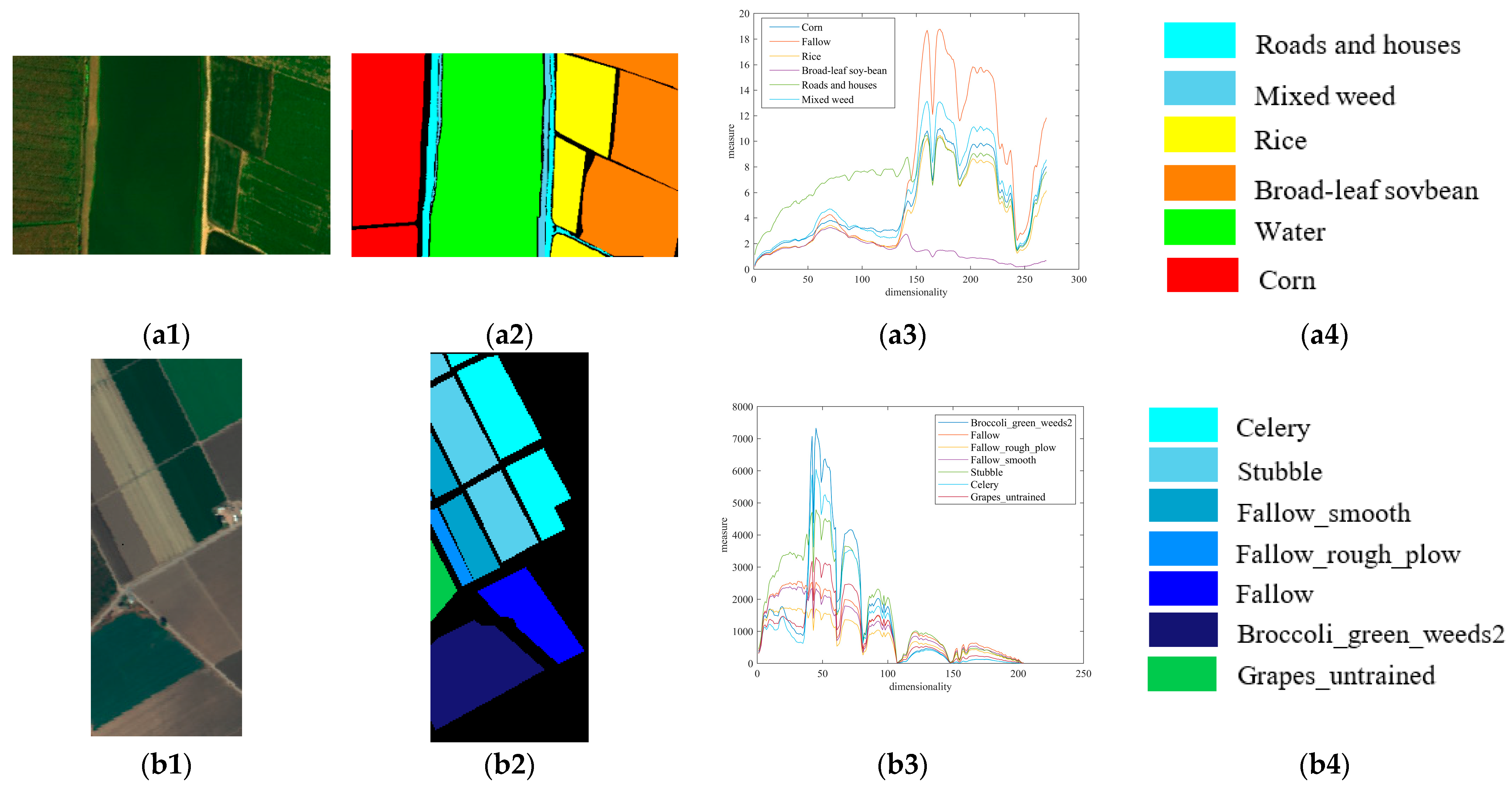
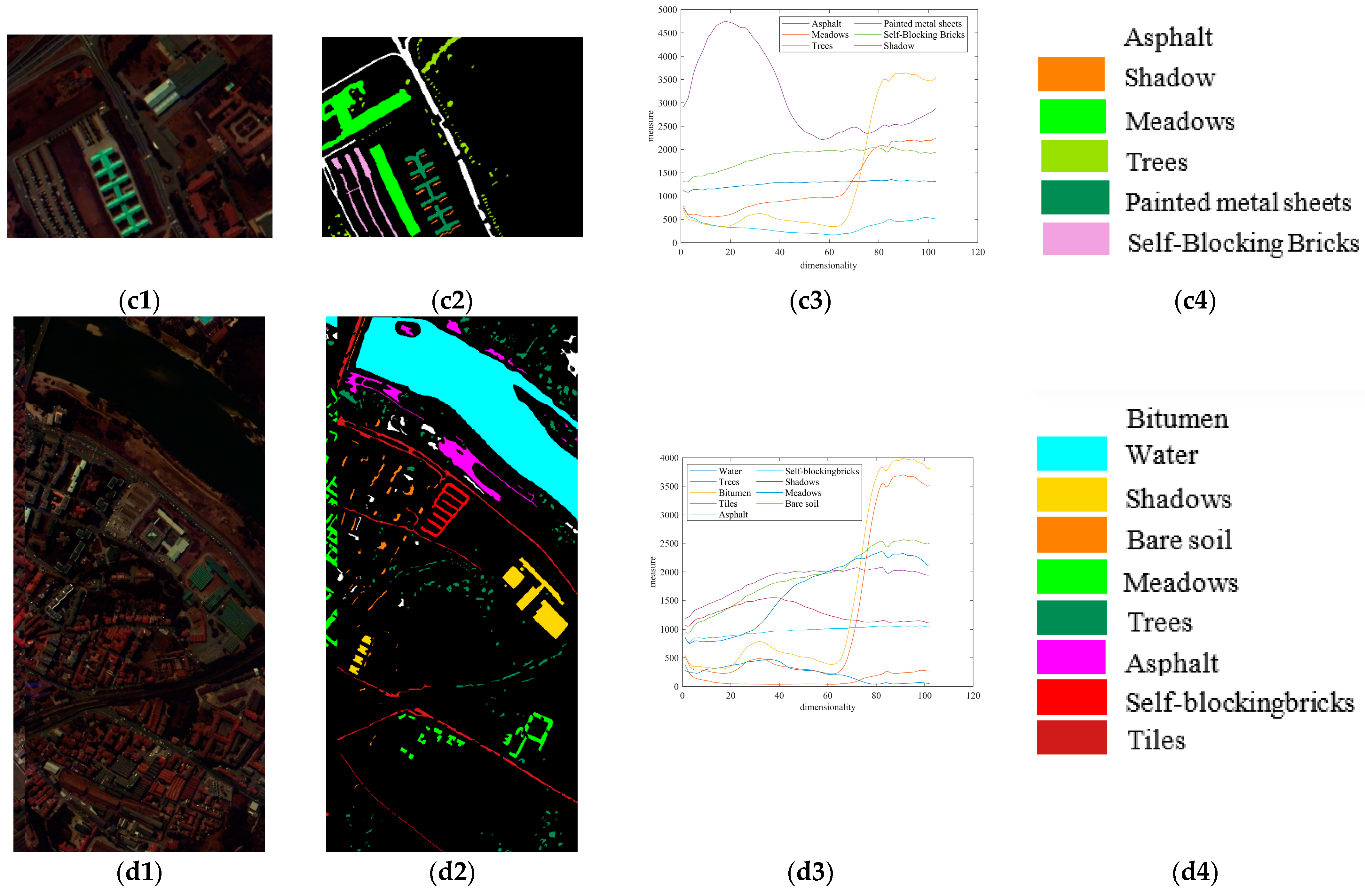
This paper uses four publicly available datasets with validation data, namely, the real LongKou [40,41], Salinas, Pavia University, and Pavia Centre images. Among them, the LongKou images are obtained by the UAV-borne hyperspectral system, and the images of Salinas, Pavia University, and Pavia Centre are obtained by the airborne hyperspectral platform. Compared with the airborne hyperspectral platform, the hyperspectral images obtained by the UAV-borne hyperspectral system have higher spatial resolutions. In addition, the standard classification data are included in the experimental data, which can effectively measure the effectiveness of the proposed algorithm. Figure 1 is an experimental image, where Figure 1(a1–d1) are false-color images, Figure 1(a2–d2) are standard classified images, Figure 1(a3–d3) are mean spectral curves for each class, and Figure 1(a4–d4) are legends for all classes of four real images. The experimental image parameters are shown in Table 1.
As some data points in the four experimental images do not contain any information, these data points are regarded as background and discarded before application. The numbers of spectral vectors of these hyperspectral remote sensing images are 93083, 14879, 11915, and 107352, respectively.

3. The Proposed Algorithm

First, the TRP algorithm is used to reduce the dimensions of hyperspectral remote sensing images containing all bands. Then, the MD classifier is used to classify the low-dimensional images to obtain the distance matrix. Finally, they are included in the ensemble classification framework to obtain the final classification results.

3.1. TRP Algorithm

Given a hyperspectral remote sensing image A = {aj, j = 1, …, J}, where j is the pixel index, J is the number of pixels, and aj = (ajd, d = 1, …, D) is the spectral measure vector of pixel j, d is the band index, D is the number of bands, and ajd is the spectral measure of the band d of pixel j. Taking the spectral vector aj (j = 1, …, J) as the row vector, a hyperspectral remote sensing image can be expressed as a J × D matrix. For the convenience of description, A is still used to refer to a hyperspectral remote sensing image matrix without confusion, that is, A = [a1, … aj, …, aJ]T, where T is the transpose operation.
The TRP algorithm can project hyperspectral remote sensing images into a low-dimensional subspace and make any vector pair in the low-dimensional subspace satisfy the distance relative invariance with a high probability. It is possible for the TRP algorithm to reduce the dimensionality of hyperspectral remote sensing images. The TRP algorithm is as follows [31].
Theorem 1.
The D dimensional feature space can be randomly projected into the KTRP dimensional space, where KTRP is a positive integer and satisfies,
K TRP K TRP 0 = 320 + 160 β ε + 20 ε 2 ln J
where K T R P 0 is the intrinsic dimensionality, ⌈ ⌉ is the round up character, ε ∈ [0.7, 1.5], and β > 0 are the projection parameters that control the range of distance preservation and the success rate of projection, respectively. Let RTRP = [rdk]D × KTRP be a tighter random projection matrix, and rdk are independent random variables subject to standard normal distribution, that is, rdk ~ N(0, 1). For a given hyperspectral remote sensing image A, the low-dimensional image B projected to KTRP dimensionality by RTRP is,
B = 1 K TRP A R TRP
where B = [b1, …, bj, …, bJ]T = [bjk]J × KTRP, and bj is the low-dimensional vector of pixel j. For the spectral vectors aj and aj′ in the hyperspectral remote sensing image A, let the corresponding two low-dimensional vectors in the low-dimensional image B be bj and bj′, respectively. bj and bj′ satisfy the distance relative invariance, if
( 1 ε ) α j α j 2 2 b j b j 2 2 ( 1 + ε ) α j α j 2 2
where 2 represents 2-norm. So, α j α j 2 2 = d = 1 D ( a j d a j d ) 2 Any two low-dimensional vectors in the KTRP dimensional space obtained by the TRP algorithm satisfy the distance relative invariance at least with the probability PTRP, where PTRP = 1 − J–β.
It is worth noting that the distance relative invariance is not that the square of the distance between the vectors before and after projection is equal, but b j b j 2 2 remains at interval [ ( 1 ε ) α j α j 2 2 , ( 1 + ε ) α j α j 2 2 ] . The bj and bj with b j b j 2 2 out of the interval [ ( 1 ε ) α j α j 2 2 , ( 1 + ε ) α j α j 2 2 ] are considered to have little similarity of the vector pair before and after projection. Under the constraint of the same probability PTRP, the intrinsic dimensionality of the TRP algorithm is lower than that of the RP algorithm. Therefore, the TRP algorithm can reduce the number of bands in hyperspectral remote sensing images to a greater extent, while ensuring that the vector pairs satisfy the distance relative invariance with probability PTRP. As distance reflects the structure of the dataset, the TRP algorithm indicates that low-dimensional images in a low-dimensional space can maintain the structure of hyperspectral remote sensing images with a high probability.
The detailed process of the TRP Algorithm 1 can be summarized as follows.
Algorithm 1. The detailed process of the TRP algorithm.
Input: test hyperspectral remote sensing image A.
Output: low-dimensional image B.
Step 1. Calculate K TRP 0 ← Equation (1), and set the dimensionality KTRP.
Step 2. Generate rdk according to the standard normal distribution, that is rdk ~ N(0, 1).
Step 3. Form R.
Step 4. Calculate the low-dimensional image B ← Equation (2).

3.2. Random Projection Matrix Selection Strategy

The random projection matrix is randomly generated without considering the class information of hyperspectral remote sensing images. Different random projection matrices will produce different low-dimensional images. Therefore, the selection of the random projection matrix directly affects the subsequent classification accuracy of hyperspectral remote sensing images. To make low-dimensional images have stronger class separability and achieve accurate classification of hyperspectral remote sensing images, this subsection uses a random projection matrix selection strategy based on the separable information of a single class to obtain low-dimensional images with the best separability of a single class. It is worth noting that the benefit of subsequent classification refers to greater differences between classes and smaller differences within classes. This means that there may be overtraining effects and generalization may degenerate, but it is more meaningful for classification tasks.
First, the sample matrix of all classes is defined as F = [F1; …; Fl; …; FL], where l is the class index, Fl is the sample matrix of the lth class, and L is the number of classes, which is a priori. It can be specifically expressed as
F l = [ f 11 l f 12 l f 1 D l f 21 l f 22 l f 2 D l f H 1 l f H 2 l f H D l ] = [ F 1 l F 2 l F D l ]
where F d l is the sample vector of the lth class and the dth (d = 1, 2, , D) band, and H is the number of samples of the lth class. It is worth noting that this paper sets the number of samples to be the same for all classes. Then, the TRP algorithm is used to reduce the dimensionality of the samples. Through the random projection matrix R, the sample matrix F of all classes can be projected into the KTRP dimensional space, thereby obtaining the low-dimensional sample matrix S = [S1; …; Sl; …; SL] of all classes. It is calculated as follows,
S = 1 K TRP   F R TRP
SL in the S matrix is the low-dimensional sample matrix of the lth class obtained by using the TRP algorithm for dimensionality reduction. The specific expansion is as follows:
S l = [ s 11 l s 12 l s 1 K TRP l s 21 l s 22 l s 2 K TRP l s H 1 l s H 2 l s H K TRP l ] = [ s 1 l s 2 l s K TRP l ]
where s H 1 l is the low-dimensional measure of the first dimensionality of Hth sample of lth class, and s k l is the low-dimensional sample vector of the kth dimensionality in the KTRP dimensional space,
s k l = [ s 1 k l s 2 k l s H k l ] = r 1 k [ f 11 l f 21 l f H 1 l ] + r 2 k [ f 12 l f 22 l f H 2 l ] + + r D k [ f 1 D l f 2 D l f H D l ] = r 1 k F 1 l + r 2 k F 2 l + + r D k F D l = d = 1 D r d k F d l
According to Equation (7), s k l is related to the vector rk of the kth column in the random projection matrix. Thus, each element rdk in the kth column of the random projection matrix can be limited by constraining each cumulative sum of s k l . The random projection matrix with the best class separability of the dimensionality reduction result can be selected by means of multiple sampling.
The measurement of the random projection matrix selection strategy based on the separable information of a single class is the large intra-class variance of a single class and the small distance from other classes. Each dimensionality in the random projection matrix is separately selected, to select the random projection matrix that is extremely conducive to the classification of this class.
As each element rdk of the random projection matrix R obeys the standard normal distribution, multiple random numbers can be generated according to this distribution as the sampling set of the elements rdk. It is defined as Qdk = [ Q d k 1 , …, Q d k ψ , …, Q d k Ψ ]. Each random number Q d k ψ is used to calculate the class separability, and the random number that maximizes the degree of separability of a certain class is selected as the element rdk of the random projection matrix R.
Specifically, the lth class is taken as an example to introduce the random projection matrix selection strategy based on the separable information of a single class. For the random number Q d k ψ , the variance of the lth class samples and the distance from other class samples are calculated, respectively. Then, the minimum distance between this class and other classes is divided by the variance of this class to get the lth class final difference value W d k l ψ . It can be calculated by
W d k l Ψ = m i n l = 1 , , L ( r 1 k F 1 l F 1 l 2 + + r d 1 k F d 1 l F d 1 l 2 + Q d k Ψ F d l F d l 2 ) v a r ( r 1 k F 1 l + + r d 1 k F d 1 l + Q d k Ψ F d l )
According to Equation (8), the difference matrix of this class can be obtained by using all random numbers and is expressed as W d k l ψ = [ W d k l 1 , …, W d k l ψ , …, W d k l Ψ ]. Then, the ψ*th sampling is obtained by maximizing the final difference value of the lth class, that is,
ψ * = arg max ψ = 1 ,   ,   Ψ { G d k ψ }
Finally, the element rdk takes the ψ*th sampling random number that maximizes the final class difference value, that is,
r d k = Q d k ψ *

3.3. Entropy-Weighted Ensemble Algorithm

The random projection matrix selection strategy based on the separable information of a single class considers the separability of a single object class but does not measure the class separability of low-dimensional images from a global perspective. To this end, based on the idea of the random projection matrix selection strategy of the separable information of a single class and ensemble classification, the classification results of multiple low-dimensional images are combined to construct a classification model, thereby obtaining more stable and accurate classification results.
The main idea of the entropy-weighted ensemble classification algorithm is to use the random projection matrix selection strategy based on the separable information of a single class to select L random projection matrices suitable for L classes, respectively. In addition, the TRP algorithm is used to reduce the dimensionality of the hyperspectral remote sensing images A based on these projection matrices, thereby obtaining L low-dimensional images. The number of ensembles is set as the number of classes in this paper to ensure that each class is considered. For ease of reference, iter is used to represent the index of ensembles, that is, iter = 1, …, L. The low-dimensional image obtained by the iterth ensemble using the TRP algorithm is defined as Biter.
The MD classifier is used to classify L low-dimensional images to obtain L distance matrices, respectively. Each distance matrix Ziter is regarded as a similarity measurement matrix between the low-dimensional spectral vector and the mean vector of each class. Finally, the entropy information is used to weigh each matrix to obtain the final similarity measure matrix C.
With the help of the class information of the samples, the TRP algorithm is used to calculate the lower limit of the projection dimension KTRP, and the random projection matrix Riter is obtained by the random projection matrix selection strategy. Then, the sample matrix F of all classes can be projected into the KTRP dimensional space. The result of the dimensionality reduction of the sample matrix F by the random projection matrix Riter is Siter = [Siter1; …; Siterl; …; SiterL], which is calculated as follows
S i t e r = 1 K TRP   F R i t e r
Then the feature mean vector S mean i t e r l of the low-dimensional samples of the lth class is calculated to obtain distance matrix, which is expressed as
S mean i t e r l = 1 H S i t e r l = 1 H [ s 11 i t e r + + s H 1 i t e r , s 12 i t e r + + s H 2 i t e r , , s 1 K T R P i t e r + + s H K T R P i t e r ]
Then, according to Equation (11), the same random projection matrix Riter is used to reduce the dimensionality of the hyperspectral remote sensing image A to obtain the low-dimensional image Biter. So far, the feature mean vector and low-dimensional images of all classes of low-dimensional samples can be obtained. The MD classifier builds a classification model on low-dimensional images, and the similarity of the low-dimensional vector is defined by calculating the distance between each low-dimensional vector and the mean vector of each class sample. The distance matrix is defined as Ziter = [ z 1 i t e r , …, z j i t e r , …, z J i t e r ], where z j i t e r is the distance between the jth low-dimensional vector and the mean vector of all class samples of the iterth ensemble. Specifically, z j i t e r = [ z j 1 i t e r , …, z j l i t e r , …, z j L i t e r ], where z j l i t e r is between the mean vector S mean i t e r l of the lth class low-dimensional samples and the low-dimensional vector b J i t e r . The distance is calculated as follows
z j l i t e r = S mean i t e r l b j i t e r
In the process of entropy-weighted ensemble classification, to avoid the problem that the distance value in each distance matrix is too large or too small, it is necessary to normalize each distance matrix Ziter to obtain the matrix Yiter before processing all the distance matrices, that is, Yiter = [ y 1 i t e r , …, y j i t e r , …, y J i t e r ]. Specifically, y j i t e r = [ y j 1 i t e r , …, y j l i t e r , …, y j L i t e r ], where y j l i t e r is calculated as follows
y j l i t e r = z j l i t e r min l = 1 ,   ,   L { min j = 1 ,   ,   J { z j l i t e r } } max l = 1 ,   ,   L { max j = 1 ,   ,   J { z j l i t e r } } min l = 1 ,   ,   L { min j = 1 ,   ,   J { z j l i t e r } }
The information entropy is used to perform weighted ensemble processing on multiple distance matrices to generate a similarity measure matrix, and the entropy value of the defined matrix Yiter is calculated as follows
E i t e r = g = 0 G p g i t e r ln p g i t e r
where G represents the total number of unique distance values, p g i t e r represents the probability that the distance value in iterth matrix Yiter is g, and the frequency is not 0. It can be calculated by
p g i t e r = 1 J × L # { ( j , l ) , y j l i t e r = g }
where # represents the quantity, and the (j, l) is the position where the distance value is g. The final similarity measure matrix C = {cjl, j = 1, …, J, l = 1, …, L} is calculated as follows
C = 1 L i t e r = 1 L E i t e r Y i t e r
Finally, to model the class, the deterministic classification result o = [o1, …, oj, …, oJ] can be obtained in the decision-making process of hyperspectral remote sensing images classification, where oj ∈ {1, …, L}. Simply, the low-dimensional vector bj belongs to the lth class with the smallest Euclidean distance,
o j = arg min l = 1 ,   ,   L { c j l }

3.4. The Complexity of the Proposed Algorithm

The space and time complexities of the proposed algorithm are analyzed here. This section studies the complexity in three parts: the optimization strategy of the projection matrix, the MD classifier, and the ensemble algorithm.
The main contribution of the complexity of the optimization strategy of the projection matrix is to calculate the projection matrix. To update the projection matrix, it takes O(HLD) space and O(HLDKTRP) time for the calculation of the low-dimensional sample matrix. Furthermore, O(HKTRP) space and O(THL2KTRP) time are required to calculate the class dissimilarity. The main contribution of the complexity of the classification algorithm is to calculate the distance matrix. To update the distance matrix, it takes O(SD) space and O(SDKTRP) time for the calculation of the low-dimensional images. Furthermore, O(SKTRP) space and O(SLKTRP) time are required to calculate the distance. The main contribution of the complexity of the ensemble algorithm is to repeat the above two steps. To obtain the final distance matrix, the overall space complexity of the proposed algorithm is O(LSD), and the overall time complexity of the proposed algorithm is O(L(HLDKTRP + THL2KTRP + SDKTRP + SLKTRP)).
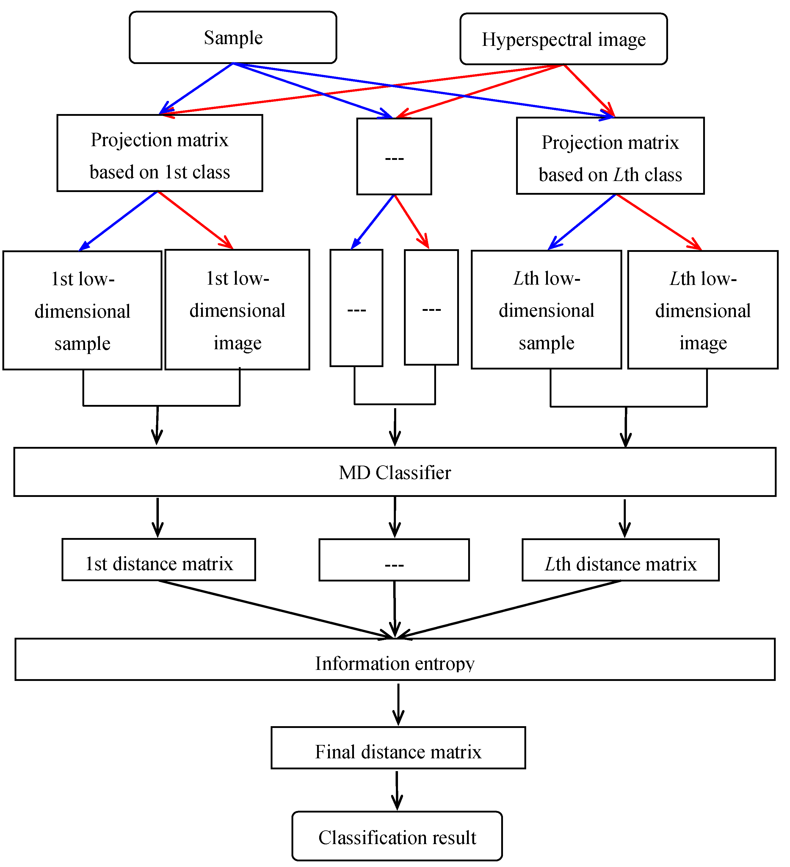
Figure 2 presents the flow chart for the proposed algorithm. For easier understanding, the blue arrows represent the dimensionality reduction process of samples, and the red arrows represent the dimensionality reduction process of hyperspectral remote sensing images.
Furthermore, the detailed process of the proposed Algorithm 2 can be summarized as follows.
Algorithm 2. The detailed process of the proposed classification algorithm.
Input: samples F, test hyperspectral remote sensing image A.
Output: the classification results o.
Step 1. Calculate K TRP 0 ← Equation (1), and set the dimensionality KTRP.
For iter = 1: L
  Step 2. Randomly generate Ψ random numbers according to the standard normal distribution.
  Step 3. Calculate the final difference value W d k l ψ ← Equation (8).
  Step 4. Calculate the ψ*th sampling ← Equation (9).
  Step 5. Form Riter ← Equation (10).
  Step 6. Reduce the dimensionality of the hyperspectral image A and samples F ← Equation (11).
  Step 7. Calculate the mean vector of each low-dimensional class sample ← Equation (12).
  Step 8. Calculate distance matrix Ziter ← Equation (14).
End
Step 9. Obtain the entropy value Eiter ← Equation (15).
Step 10. Obtain the final similarity measure matrix C ← Equation (17).
Step 11. Make a classification decision o ← Equation (18).

4. Results and Discussion

To verify the superiority of the proposed classification algorithm, MATLAB R2018a software is used to classify real hyperspectral remote sensing images on a computer with Intel (R) Core (TM) i5-4460, 3.20 GHz, 8 GB memory. The results are qualitatively and quantitatively evaluated. In this paper, four sets of real hyperspectral remote sensing images with different spectral and spatial resolutions are shown in Figure 1. In addition, this paper mainly considers the amount of calculation and sets the projection parameters as ε = 1.5 and β = 0.5 for the four experimental images. For the sake of fairness, the projection parameters of all experimental images are set uniformly, and their parameters are shown in Table 2. The projection dimensionalities of the TRP algorithm in Table 2 are set as the intrinsic dimensionality, which is based on Equation (1) in the projection parameters ε = 1.5 and β = 0.5. It is worth noting that the projection dimensionality of the TRP algorithm in Table 2 is at least one-third that of the RP algorithm, greatly reducing the computational complexity.
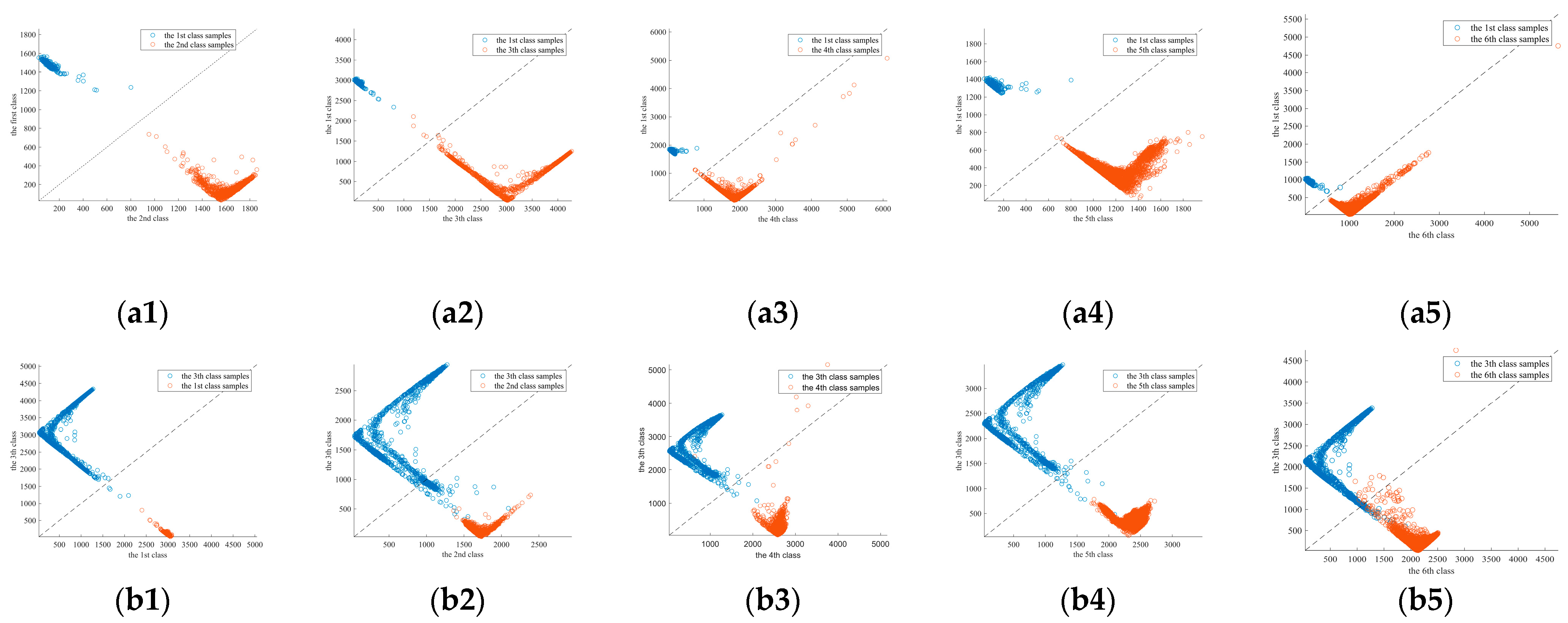
To validate the effectiveness of the random projection matrix selection strategy, the nonlinear projection method [42] was used to visualize class separability. As this method displays the separability of two classes in a two-dimensional space, the class separability of spectral vectors before and after dimensionality reduction in the Pavia University image was analyzed. The first and second lines in Figure 3 show the visualization results of the first and third ensembles, respectively. Among those, the horizontal and vertical coordinates in the visualization results represent the distance from the spectral vector to the mean vector of the two classes of samples, respectively. The blue and red circles represent the distance distribution of the two classes of spectral vectors, respectively. The black dashed line is the dividing line for measuring the class separability, that is a straight line at a 45-degree angle passing through the origin. The more spectral vectors scattered on both sides, the better the class separability of the dimensionality reduction results. From Figure 3, the spectral vectors are almost completely scattered on both sides of the dividing line, and most of them are close to the coordinate axis. This indicates that there are many correctly classified spectral vectors.
To prove the superiority of the proposed algorithm, TRP-MIV, the SVM classification algorithm based on LDA (hereinafter referred to as LDA-SVM) and the CAFCM classification algorithm are used to classify these hyperspectral remote sensing images. The classification results are qualitatively and quantitatively evaluated. The parameters of comparison algorithms are shown in Table 3. In addition, all experimental images are tested 100 times to effectively evaluate the classification accuracy.
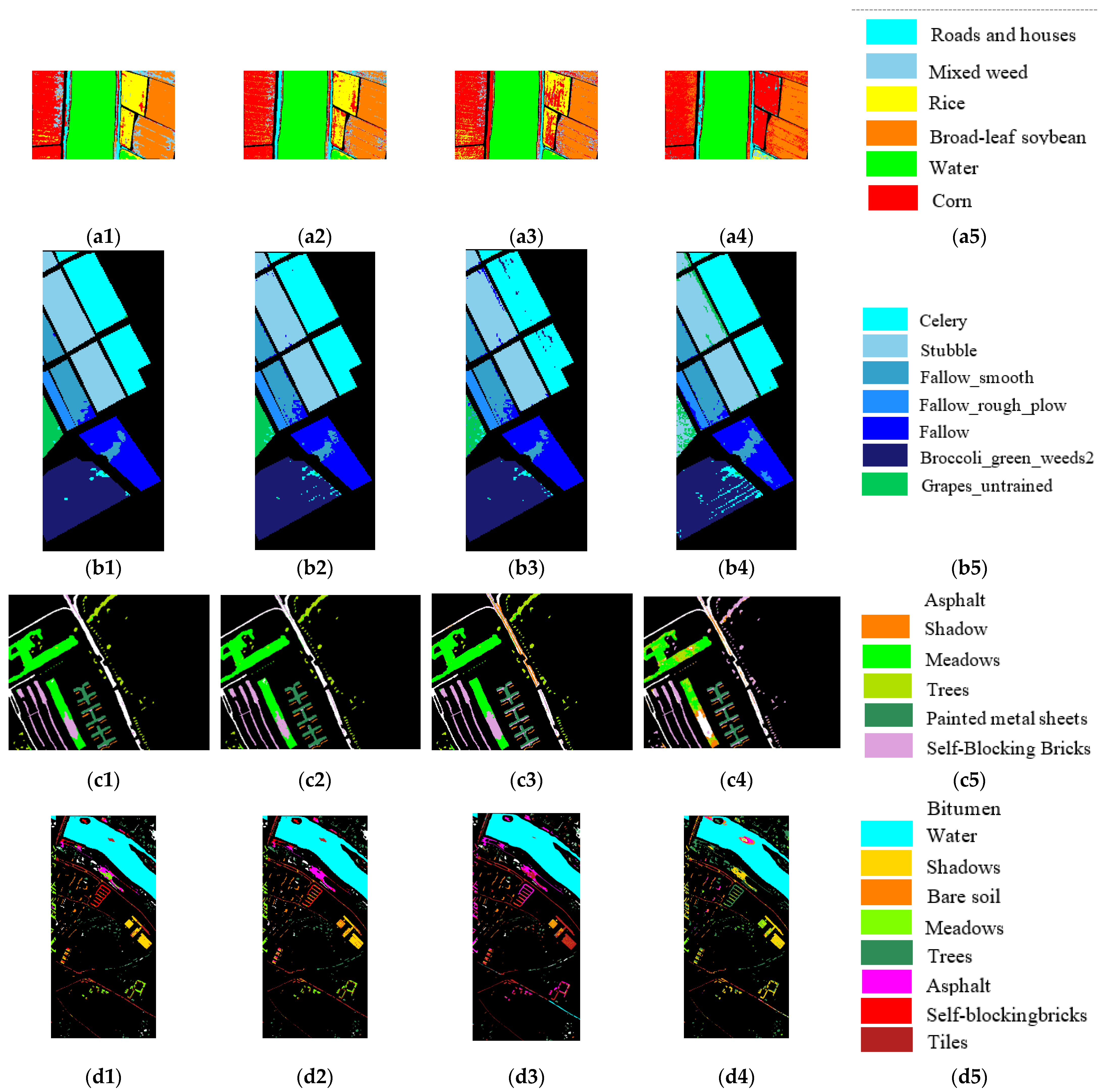
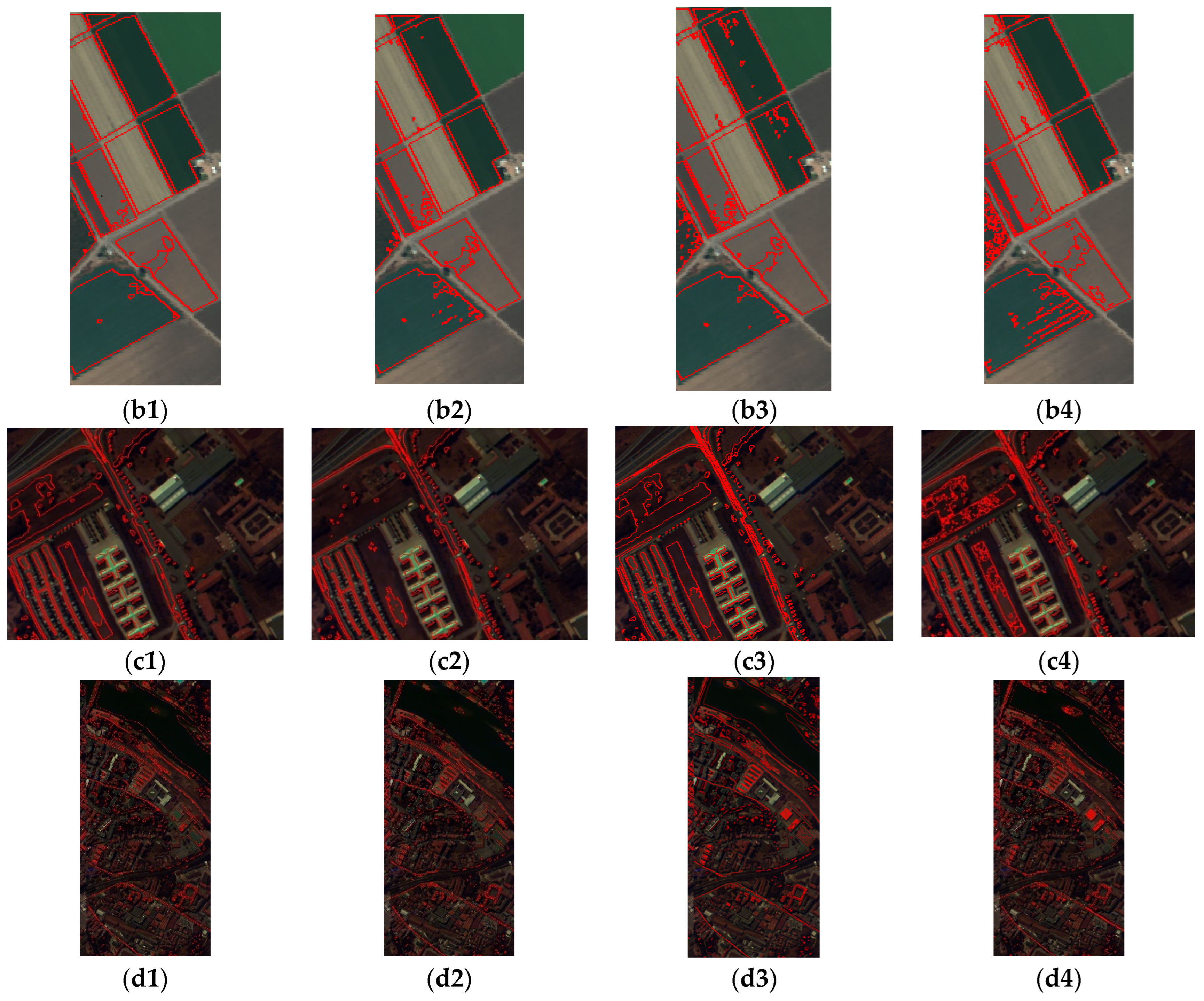
The experimental results are shown in Figure 4. Figure 4 shows the best classification results in 100 trials of the LongKou, Salinas, Pavia University, and Pavia Centre images, respectively. In addition, to qualitatively evaluate the above classification results, the contour lines between the regions in the classification results are extracted and superimposed on the corresponding false color images, and the superposition results are shown in Figure 5.
Through visual evaluation, it can be concluded that the contours of each region in the contour stacking result of the proposed algorithm can coincide well with the boundaries of each class region in the false color images. For images with large intra-class variances (for example, the Salinas and Pavia University images), the proposed algorithm can still obtain better classification results despite misclassification. Since the proposed algorithm can maintain the separability of each class, the algorithm can perform a fine classification of each class. Since the TRP-MIV algorithm selects the random projection matrix based on the separable information of all classes, the features of some classes are always ignored. There are several speckle noises in the classification results of the LDA-SVM algorithm, especially in the Pavia Centre image where there is still misclassification. It can be seen from Figure 4 and Figure 5 that the missed classification of the CAFCM classification algorithm is profoundly serious, and the spectral vectors in the same class are incorrectly classified into other classes. For complex texture images, the CAFCM algorithm is easily disturbed by noise, so it cannot obtain ideal classification results. All information shows that the proposed algorithm can classify hyperspectral remote sensing images well.
In order to quantitatively evaluate the classification results of the proposed algorithm, the confusion matrix of the classification results is obtained by taking Figure 2(a2–d2) as the standard classification data, and the Overall Accuracy (OA), Average Accuracy (AA), Average Precision Rate (APR), and the Kappa coefficient of the whole classification result are calculated according to the confusion matrix. Meanwhile, the runtime of all images was quantitatively analyzed. Table 4, Table 5, Table 6 and Table 7 are the accuracy evaluations of the classification results of the four images, respectively. Additionally, the values in Table 4, Table 5, Table 6 and Table 7 are the mean values of 100 trials, where the unit of running time is seconds.
The mean values of OA, AA, APR, and the Kappa coefficient of the proposed algorithm for the four experimental images are greater than 87%, 80%, 78%, and 0.84, respectively. The OA, AA, APR, and the Kappa values of the comparison algorithms are all lower than those of the proposed algorithm, which means that the proposed algorithm can obtain higher accuracy classification results than the comparison algorithms. Since the TRP-MIV algorithm does not need to perform multiple projections, the running time of the TRP-MIV algorithm is shorter than that of the proposed algorithm. Nonetheless, as can be seen from the running time in Table 4, Table 5, Table 6 and Table 7, the proposed algorithm can obtain high classification accuracy in an acceptable time. In addition, the classification accuracy variance value of the proposed algorithm for 100 trials, which is the value in brackets, is smaller than those of the comparison algorithms, which fully shows that the proposed algorithm is robust. All the classification accuracies show that the proposed algorithm can obtain very good classification results.
Based on the above discussion, by comparing the visual and quantitative evaluations of the proposed classification algorithm and the comparison algorithms, the proposed algorithm outperforms the comparison algorithms in classification performance and stability but is slightly inferior to the comparison algorithms in algorithm running time.

5. Conclusions

Aiming to resolve the problem that the randomness of the RP algorithm may lead to unstable classification results, TRP-oriented hyperspectral remote sensing image classification using an entropy-weighted ensemble algorithm is proposed. Additionally, the classification experiments are conducted on real hyperspectral remote sensing images. The proposed algorithm can effectively improve the classification accuracy and robustness of hyperspectral remote sensing images. The classes with poor separability can also be better distinguished, which basically meets the task of classifying hyperspectral remote sensing images completely and finely. The following points should be completed in the following work. The choice of projection dimensionality in this paper is based on the principle of computational cost. The influence of projection dimensionality on classification accuracy is the research direction.

Author Contributions

Conceptualization, S.J., Y.L. and Q.Z.; methodology, S.J., Y.L. and Q.Z.; software, S.J.; validation, S.J.; formal analysis, S.J. and C.W.; writing—original draft preparation, S.J.; writing—review and editing, S.J. and C.W. All authors have read and agreed to the published version of the manuscript.

Funding

This research was funded by the Natural Science Foundation of Liaoning 2022, grant number 2022-MS-400.

Data Availability Statement

The data presented in this study are openly available at http://www.ehu.eus/ccwintco/index.php/Hyperspectral_Remote_Sensing_Scenes accessed on 12 July 2021 and http://rsidea.whu.edu.cn/resource_WHUHi_sharing.htm accessed on 1 October 2020.

Acknowledgments

The authors would like to thank Gamba P. for providing the ROSIS Pavia University and Pavia Centre data, Johnson L. and Gualtieri J. A. for providing the AVIRIS Salinas data, and the Intelligent Data Extraction, Analysis and Applications of Remote Sensing (RSIDEA) academic research group, State Key Laboratory of Information Engineering in Surveying, Mapping, and Remote Sensing (LIESMARS), Wuhan University, for providing the LongKou data.

Conflicts of Interest

The authors declare no conflict of interest.

References

  1. Gao, P.; Zhang, H.; Yu, J.; Lin, J.; Wang, X.; Yang, M.; Kong, F. Secure Cloud-Aided Object Recognition on Hyperspectral Remote Sensing Images. IEEE Internet Things J. 2020, 8, 3287–3299. [Google Scholar] [CrossRef]
  2. Li, H.; Cui, J.; Zhang, X.; Han, Y.; Cao, L. Dimensionality Reduction and Classification of Hyperspectral Remote Sensing Image Feature Extraction. Remote Sens. 2022, 14, 4579. [Google Scholar] [CrossRef]
  3. Bera, S.; Shrivastava, V.K. Analysis of various optimizers on deep convolutional neural network model in the application of hyperspectral remote sensing image classification. Int. J. Remote Sens. 2019, 41, 2664–2683. [Google Scholar] [CrossRef]
  4. Lei, R.; Zhang, C.; Liu, W.; Zhang, L.; Zhang, X.; Yang, Y.; Huang, J.; Li, Z.; Zhou, Z. Hyperspectral Remote Sensing Image Classification Using Deep Convolutional Capsule Network. IEEE J. Sel. Top. Appl. Earth Obs. Remote Sens. 2021, 14, 8297–8315. [Google Scholar] [CrossRef]
  5. Xiao, Z.; Bourennane, S. Constrained nonnegative matrix factorization and hyperspectral image dimensionality reduction. Remote Sens. Lett. 2014, 5, 46–54. [Google Scholar] [CrossRef]
  6. Deng, Y.-J.; Li, H.-C.; Fu, K.; Du, Q.; Emery, W.J. Tensor Low-Rank Discriminant Embedding for Hyperspectral Image Dimensionality Reduction. IEEE Trans. Geosci. Remote Sens. 2018, 56, 7183–7194. [Google Scholar] [CrossRef]
  7. Wang, P.; Zheng, C.; Xiong, S. Hyperspectral Image Dimensionality Reduction via Graph Embedding in Core Tensor Space. IEEE Geosci. Remote Sens. Lett. 2020, 18, 509–513. [Google Scholar] [CrossRef]
  8. Singh, P.S.; Karthikeyan, S. Enhanced classification of remotely sensed hyperspectral images through efficient band selection using autoencoders and genetic algorithm. Neural Comput. Appl. 2021, 34, 21539–21550. [Google Scholar] [CrossRef]
  9. Shi, J.; Zhang, X.; Liu, X.; Lei, Y.; Jeon, G. Multicriteria semi-supervised hyperspectral band selection based on evolutionary multitask optimization. Knowl.-Based Syst. 2022, 240, 107934. [Google Scholar] [CrossRef]
  10. Paul, A.; Chaki, N. Band selection using spectral and spatial information in particle swarm optimization for hyperspectral image classification. Soft Comput. 2022, 26, 2819–2834. [Google Scholar] [CrossRef]
  11. Yin, J.; Gao, C.; Jia, X. Using Hurst and Lyapunov Exponent For Hyperspectral Image Feature Extraction. IEEE Geosci. Remote Sens. Lett. 2012, 9, 705–709. [Google Scholar] [CrossRef]
  12. Yuan, H.; Tang, Y.Y. Learning with Hypergraph for Hyperspectral Image Feature Extraction. IEEE Geosci. Remote Sens. Lett. 2015, 12, 1695–1699. [Google Scholar] [CrossRef]
  13. Xie, W.; Lei, J.; Fang, S.; Li, Y.; Jia, X.; Li, M. Dual feature extraction network for hyperspectral image analysis. Pattern Recognit. 2021, 118, 107992. [Google Scholar] [CrossRef]
  14. Huang, H.-Y.; Kuo, B.-C. Double Nearest Proportion Feature Extraction for Hyperspectral-Image Classification. IEEE Trans. Geosci. Remote Sens. 2010, 48, 4034–4046. [Google Scholar] [CrossRef]
  15. Zhao, K.; Valle, D.; Popescu, S.; Zhang, X.; Mallick, B. Hyperspectral remote sensing of plant biochemistry using Bayesian model averaging with variable and band selection. Remote Sens. Environ. 2013, 132, 102–119. [Google Scholar] [CrossRef]
  16. Vempala, S.S. The Random Projection Method; American Mathematical Society: Providence, RI, USA, 2004. [Google Scholar] [CrossRef]
  17. Li, P.; Trevor, J.H.; Kenneth, W.C. Very sparse random projections. In Proceedings of the 2006 12th ACM SIGKDD International Conference on Knowledge Discovery and Data Mining, Philadelphia, PA, USA, 20–23 August 2006; Association for Computing Machinery: New York, NY, USA, 2006; pp. 287–296. [Google Scholar] [CrossRef]
  18. Johnson, W.B.; Lindenstrauss, J.; Schechtman, G. Extensions of Lipschitz maps into Banach spaces. Israel J. Math. 1986, 54, 129–138. [Google Scholar] [CrossRef]
  19. Johnson, W.B.; Lindenstrauss, J. Extensions of Lipschitz mappings into a Hilbert space. Contemp. Math. 1984, 26, 189–206. [Google Scholar] [CrossRef]
  20. Menon, A.K. Random Projections and Applications to Dimensionality Reduction. Bachelor’s Thesis, The University of Sydney, Darlington, Australia, March 2007. [Google Scholar]
  21. Ravazzi, C.; Fosson, S.; Bianchi, T.; Magli, E. Sparsity estimation from compressive projections via sparse random matrices. EURASIP J. Adv. Signal Process 2018, 2018, 56. [Google Scholar] [CrossRef]
  22. Najarzadeh, D. A simple test for zero multiple correlation coefficient in high-dimensional normal data using random projection. Comput. Stat. Data Anal. 2020, 148, 106955. [Google Scholar] [CrossRef]
  23. Wu, H.; Dai, S.; Liu, C.; Wang, A.; Iwahori, Y. A Novel Dual-Encoder Model for Hyperspectral and LiDAR Joint Classification via Contrastive Learning. Remote Sens. 2023, 15, 924. [Google Scholar] [CrossRef]
  24. Zhang, J.; Shao, M.; Wan, Z.; Li, Y. Multi-Scale Feature Mapping Network for Hyperspectral Image Super-Resolution. Remote Sens. 2021, 13, 4180. [Google Scholar] [CrossRef]
  25. Huang, W.; Wong, P.K.; Wong, K.I.; Vong, C.M.; Zhao, J. Adaptive neural control of vehicle yaw stability with active front steering using an improved random projection neural network. Veh. Syst. Dyn. 2019, 59, 396–414. [Google Scholar] [CrossRef]
  26. Zhou, G.; Bao, X.; Ye, S.; Wang, H.; Yan, H. Selection of Optimal Building Facade Texture Images From UAV-Based Multiple Oblique Image Flows. IEEE Trans. Geosci. Remote Sens. 2020, 59, 1534–1552. [Google Scholar] [CrossRef]
  27. Qiu, Z.; Yue, L.; Liu, X. Void Filling of Digital Elevation Models with a Terrain Texture Learning Model Based on Generative Adversarial Networks. Remote Sens. 2019, 11, 2829. [Google Scholar] [CrossRef]
  28. Jin, B.; Cruz, L.; Goncalves, N. Pseudo RGB-D Face Recognition. IEEE Sens. J. 2022, 22, 21780–21794. [Google Scholar] [CrossRef]
  29. Zhou, G.; Yang, F.; Xiao, J. Study on Pixel Entanglement Theory for Imagery Classification. IEEE Trans. Geosci. Remote Sens. 2022, 60, 3167569. [Google Scholar] [CrossRef]
  30. Zheng, Q.; Zhao, P.; Li, Y.; Wang, H.; Yang, Y. Spectrum interference-based two-level data augmentation method in deep learning for automatic modulation classification. Neural Comput. Appl. 2020, 33, 7723–7745. [Google Scholar] [CrossRef]
  31. Zhao, Q.; Jia, S.; Li, Y. Hyperspectral remote sensing image classification based on tighter random projection with minimal intra-class variance algorithm. Pattern Recognit. 2020, 111, 107635. [Google Scholar] [CrossRef]
  32. El-Shishiny, H.; Abdel-Mottaleb, M.; El-Raey, M.; Shoukry, A. A multistage algorithm for fast classification of patterns. Pattern Recognit. Lett. 1989, 10, 211–215. [Google Scholar] [CrossRef]
  33. Zhao, R.; Mao, K. Semi-Random Projection for Dimensionality Reduction and Extreme Learning Machine in High-Dimensional Space. IEEE Comput. Intell. Mag. 2015, 10, 30–41. [Google Scholar] [CrossRef]
  34. Schclar, A.; Rokach, L. Random Projection Ensemble Classifiers. In Proceedings of the 2019 International Conference on Enterprise Information Systems, Prague, Czech Republic, 3–5 May 2009; Springer: Berlin/Heidelberg, Germany, 2009; pp. 309–316. [Google Scholar] [CrossRef]
  35. Fowler, J.E.; Du, Q.; Zhu, W.; Younan, N.H. Classification performance of random-projection-based dimensionality reduction of hyperspectral imagery. Geosci. Remote Sens. Symp. 2009, 5, V-76–V-79. [Google Scholar] [CrossRef]
  36. Pasunuri, R.; Venkaiah, V.C.; Srivastava, A. Clustering High-Dimensional Data: A Reduction-Level Fusion of PCA and Random Projection: IC3 2018; Recent Developments in Machine Learning and Data Analytics; AISC: Lviv, Ukraine, 2019. [Google Scholar] [CrossRef]
  37. Alshamiri, A.K.; Singh, A.; Surampudi, B.R. Combining ELM with Random Projections for Low and High Dimensional Data Classification and Clustering. In Proceedings of the 2015 5th International Conference on Fuzzy and Neuro Computing (FANCCO-2015), Hyderabad, India, 17–19 December 2015; Springer: Cham, Switzerland; pp. 89–107. [Google Scholar] [CrossRef]
  38. Rathore, P.; Bezdek, J.C.; Erfani, S.M.; Rajasegarar, S.; Palaniswami, M. Ensemble Fuzzy Clustering Using Cumulative Aggregation on Random Projections. IEEE Trans. Fuzzy Syst. 2017, 26, 1510–1524. [Google Scholar] [CrossRef]
  39. Anderlucci, L.; Fortunato, F.; Montanari, A. High-Dimensional Clustering via Random Projections. J. Classif. 2021, 39, 191–216. [Google Scholar] [CrossRef]
  40. Zhong, Y.; Hu, X.; Luo, C.; Wang, X.; Zhao, J.; Zhang, L. WHU-Hi: UAV-borne hyperspectral with high spatial resolution (H2) benchmark datasets and classifier for precise crop identification based on deep convolutional neural network with CRF. Remote Sens. Environ. 2020, 250, 112012. [Google Scholar] [CrossRef]
  41. Zhong, Y.; Wang, X.; Xu, Y.; Wang, S.; Jia, T.; Hu, X.; Zhao, J.; Wei, L.; Zhang, L. Mini-UAV-Borne Hyperspectral Remote Sensing: From Observation and Processing to Applications. IEEE Geosci. Remote Sens. Mag. 2018, 6, 46–62. [Google Scholar] [CrossRef]
  42. Chen, J.; Jin, Y.; Ma, S. The Visualization Analysis of Handwritten Chinese Characters in Their Feature Space. J. Chin. Inf. Process. 2000, 14, 42–48. [Google Scholar] [CrossRef]
Figure 1. Real images. (a1d1) represent the false-color images of the LongKou, Salinas, Pavia Centre, and Pavia University images, respectively. (a2d2) represent the standard classified images (i.e., validation data) of four real images, respectively. (a3d3) represent the mean spectral curves for each class. (a4d4) represent the legends for all classes of four real images, respectively.
Remotesensing 15 02315 g001aRemotesensing 15 02315 g001b
Figure 2. Flow chart of the proposed classification algorithm in this paper.
Remotesensing 15 02315 g002
Figure 3. Visualization results of the first and third ensembles of the Pavia University image. (a1a5) Visualization results of the first ensemble. (b1b5) Visualization results of the third ensemble.
Remotesensing 15 02315 g003
Figure 4. Comparison of the classification results of four images. (a1d1) The proposed algorithm. (a2–d2) The TRP-MIV algorithm. (a3d3) The LDA-SVM algorithm. (a4d4) The CAFCM algorithm. (a5d5) The legends for all classes.
Remotesensing 15 02315 g004
Figure 5. Comparison of outlines of the superposition results of four images. (a1d1) The proposed algorithm. (a2d2) The TRP-MIV algorithm. (a3d3) The LDA-SVM algorithm. (a4d4) The CAFCM algorithm. (The red lines are the outlines of the classification results.)
Remotesensing 15 02315 g005aRemotesensing 15 02315 g005b
Table 1. Parameters of experimental images.
LongKouSalinasPavia UniversityPavia Centre
Size250 × 400265 × 107260 × 3401096 × 515
Class6769
False-color bands130, 65, 1834, 18, 1168, 21, 268, 21, 2
Number of bands270204103102
Spatial resolution0.463 m3.7 m1.3 m1.3 m
SensorNano-HyperspecAVIRISROSISROSIS
Table 2. Projection parameter settings in the experiment of the proposed algorithm.
LongKouSalinasPavia UniversityPavia Centre
Ψ10101010
H10101010
KTRP998381100
KRP344289282348
Table 3. Parameter settings in the experiment of comparison algorithms.
LongKouSalinasPavia UniversityPavia Centre
TRP-MIVnumber of random numbers10101010
number of samples of each class10101010
LDA-SVMnumber of samples of each class998381100
CAFCMnumber of ensembles16941148628
Table 4. Accuracy evaluation of classification results for the LongKou image. (The values in brackets are the variance of 100 trials, and those not in are the mean).
The Proposed AlgorithmTRP-MIVLDA-SVMCAFCM
Kappa coefficient0.840.760.710.51
(0.01)(0.03)(0.01)(0.10)
OA/%87.3981.5078.4362.83
(0.65)(2.06)(0.01)(8.19)
AA/%82.3874.2959.6550.79
(1.30)(2.95)(1.71)(5.31)
APR/%81.1574.7174.6054.15
(0.47)(1.55)(0.89)(8.60)
Running time/s5.261.598.141509.77
(0.13)(0.06)(0.41)(198.36)
Table 5. Accuracy evaluation of classification results for the Salinas image. (The values in brackets are the variance of 100 trials, and those not in are the mean).
The Proposed AlgorithmTRP-MIVLDA-SVMCAFCM
Kappa coefficient0.960.940.850.71
(0.00)(0.01)(0.06)(0.09)
OA/%97.0495.0487.8676.66
(0.08)(0.76)(5.06)(7.08)
AA/%96.5494.1982.6370.99
(0.10)(1.03)(5.53)(7.56)
APR/%96.2993.74//
(0.09)(0.55)
Running time/s2.011.011.43180.51
(0.07)(0.10)(0.05)(16.17)
Table 6. Accuracy evaluation of classification results for the Pavia University image. (The values in brackets are the variance of 100 trials, and those not in are the mean).
The Proposed AlgorithmTRP-MIVLDA-SVMCAFCM
Kappa coefficient0.890.810.660.41
(0.00)(0.04)(0.06)(0.03)
OA/%92.1186.1175.0051.84
(0.27)(2.85)(3.58)(2.90)
AA/%95.0189.2875.6050.02
(0.34)(2.28)(7.28)(7.40)
APR/%92.7188.96/44.88
(0.15)(1.61)(3.53)
Running time/s0.841.211.29126.76
(0.03)(0.77)(0.15)(13.17)
Table 7. Accuracy evaluation of classification results for the Pavia Centre image. (The values in brackets are the variance of 100 trials, and those not in are the mean).
The Proposed AlgorithmTRP-MIVLDA-SVMCAFCM
Kappa coefficient0.840.800.570.36
(0.01)(0.02)(0.10)(0.09)
OA/%90.2787.8673.2952.03
(0.58)(1.10)(8.59)(9.87)
AA/%80.9374.0654.9438.82
(2.15)(3.26)(5.98)(4.71)
APR/%78.2473.0260.4734.45
(1.88)(3.09)(7.88)(5.98)
Running time/s6.551.7217.042291.91
(0.25)(0.11)(0.50)(409.44)
Disclaimer/Publisher’s Note: The statements, opinions and data contained in all publications are solely those of the individual author(s) and contributor(s) and not of MDPI and/or the editor(s). MDPI and/or the editor(s) disclaim responsibility for any injury to people or property resulting from any ideas, methods, instructions or products referred to in the content.