Article

Shoreline Analysis and Extraction Tool (SAET): A New Tool for the Automatic Extraction of Satellite-Derived Shorelines with Subpixel Accuracy

by
Jesús Palomar-Vázquez
1,
Josep E. Pardo-Pascual
1,
Jaime Almonacid-Caballer
1 and
Carlos Cabezas-Rabadán
1,2,*
1
Geo-Environmental Cartography and Remote Sensing Group, Department of Cartographic Engineering, Geodesy and Photogrammetry, Universitat Politècnica de València, Camí de Vera s/n, 46022 València, Spain
2
UMR 5805, Bordeaux INP, Université de Bordeaux-CNRS, F-33600 Pessac, France
*
Author to whom correspondence should be addressed.
Remote Sens. 2023, 15(12), 3198; https://doi.org/10.3390/rs15123198
Submission received: 2 June 2023 / Revised: 12 June 2023 / Accepted: 14 June 2023 / Published: 20 June 2023

Abstract

:
SAET (Shoreline Analysis and Extraction Tool) is a novel open-source tool to enable the completely automatic detection of shoreline position changes using the optical imagery acquired by the Sentinel-2 and Landsat 8 and 9 satellites. SAET has been developed within the ECFAS (European Coastal Flood Awareness System) project, which is intended to be the first European service for coastal flood forecasting, management, and recovery analysis. The tool is developed to characterise the shoreline response associated with punctual events such as coastal storms as well as any other phenomenon. For a given beach segment, SAET facilitates the selection of the satellite images closest in time to the analysed events that offer an adequate cloud coverage level for analysing the shoreline change. Subsequently, the tool automatically downloads the images from their official repositories, pre-processes them and extracts the shoreline position with sub-pixel accuracy. In order to do so, an initial approximate definition of the shoreline is carried out at the pixel level using a water index thresholding, followed by an accurate extraction operating on the shortwave infrared bands to produce a sub-pixel line in vector formats (points and lines). The tool offers different settings to be adapted to the different coastal environments and beach typologies. Its main advantages refer to its autonomy, its efficiency in extracting complete satellite scenes, its flexibility in adapting to different environments and conditions, and its high subpixel accuracy. This work presents an accuracy assessment on a long Mediterranean sandy beach of SDSs extracted from L8 and S2 imagery against coincident alongshore reference lines, showing an accuracy of about 3 m RMSE. At the same time, the work shows an example of the usage of SAET for characterising the response to Storm Gloria (January 2020) on the beaches of Valencia (E Spain). SAET provides an efficient and completely automatic workflow that leads to accurate SDSs while only relying on publicly available information. The tool appears to be a useful extraction tool for beach monitoring, both for public administrations and individual users.

1. Introduction

Coastal dynamism takes place at different spatial and temporal scales. In contrast to actions sustained over time that cause changes in coastal trends, punctual events can cause serious impacts on the morphology of the beaches. This is the case for anthropic actions carried out on the coast, such as the construction of infrastructure or sand nourishments [1], and the occurrence of natural events such as coastal storms. The latter constitutes a key factor controlling beach morphology as they can imply important physical modifications [2] and contribute to erosive processes. Associated with climate change and sea-level rise, the magnitude and frequency of coastal storms are expected to increase [3,4], as is the likelihood of storm surges [5] and, associated with that, their impact on the morphology of the coast.
Following storms, the resulting state of beach morphology may be unsuitable for the maintenance of beach functions [6,7]. When this happens, it may be necessary to carry out emergency actions [8] that allow the morphology to revert to a state similar to that prior to the impacts or to support the recovery process of the beach. The availability of up-to-date information on the state of the beaches before and after the storm is necessary to implement efficient management measures. Furthermore, it is also necessary to know to what extent the recovery process occurs in the longer term, thus allowing to assess the effectiveness of these measures over time and their cost–benefit for society [9]. This is not always possible due to the limitations of traditional coastal monitoring techniques, usually leading to datasets constrained to small study areas or with a low temporal resolution. To overcome these limitations, coastal monitoring studies are being increasingly supported by the use of freely available optical satellite imagery with planetary coverage and high revisit frequency [10], as well as those from the Landsat and Copernicus programs (e.g., [11,12,13]). These images offer a sub-weekly revisit time [14], which is especially important for recognizing the morphological impact of storms and their subsequent recovery as these changes can occur in a short time frame [15].
During the last years, the mapping of the water/land interface using remote sensing images acquired in the optical range of the electromagnetic spectrum has been pursued in different works (e.g., [16,17,18,19,20,21,22]). They lead to the definition of the so-called satellite-derived shorelines (SDSs) along large coastal segments and periods. This large abundance of SDS data can overcome the lack of representativeness attributed to punctual measurements that may be supplied using traditional techniques as well as provide data in areas that would otherwise not be monitored. The SDS constitutes a clear indicator of morphological changes on beaches with moderate water level changes, such as those at microtidal coasts. On the contrary, in other types of coasts, a proper interpretation of the morphological alterations of the beach may require the information provided by SDSs to be complemented by additional data such as the sea level at the instant of image acquisition and the slope of the beach face [23].
The real exploitation of satellite imagery requires tools able to characterise shoreline positions and changes robustly and accurately, covering large territories and time series. Different systems and tools such as CASSIE [24], SHOREX [25,26], and CoastSat [27] have recently been developed to obtain the satellite-derived shorelines with subpixel accuracy while attempting to integrate and simplify the different required processes. However, these tools present important differences, among which the way the image is segmented to define the land/water boundary stands out. Solutions such as CASSIE [24] or the one proposed by Hagenaars et al. [28] sustain this segmentation through the use of the normalized difference water index (NDWI; [29]). It has the advantage of using the green and near-infrared (NIR) bands, which, in the case of Sentinel-2 (S2), have a pixel size of 10 m. However, the NDWI is prone to confounding the wave foam and the emerged beach [30], forcing us to discard images with large waves even if they appear cloud-free. Thus, Hagenaars et al. [28] suggested that accurate results can only be obtained with waves with Hs < 0.5 m. CoastSAT [27] solves this limitation by pre-identifying the areas affected by foam through supervised classification. For shoreline detection, the tool employs the Modified Normalized Difference Water Index (MNDWI; [31]) that includes the short-wave infrared (SWIR-1) band, which is much less affected by this phenomenon. On the MNDWI, the tool applies a thresholding based on the method of Otsu [32], considering exclusively the spaces classified as water and sand, thus obviating the foam. Subsequently, the marching squares algorithm [33,34] interpolates on the MNDWI image the value defined by the thresholding to define the subpixel line. SHOREX [25,26] follows a completely different philosophy since, for the water/land segmentation defining an approximate line at the pixel level, it uses the automated water extraction index (AWEI; [35]), which exaggerates the differences between these two bodies. Subsequently, the sub-pixel detection is based on a neighbourhood analysis along the approximate pixel-scale line. Then, a polynomial function is fitted, and the position of the maximum gradient is detected [36] over the SWIR 1 band since it is the one that most robustly differentiates the water/land boundary [26,30].
All these tools rely on external platforms, such as Google Earth Engine (GEE), with the aim of achieving maximum efficiency by pre-processing the image in the cloud. Despite the benefits associated with its efficiency, the use of a commercial platform of this type brings conflicts for its integration into public and official services. For this reason, SAET has been designed to be able to operate completely autonomously, depending only on the official sources supplying images. In fact, SAET is a tool developed ad hoc to be integrated into ECFAS (European Coastal Flood Awareness System), a proof of concept for the implementation of a coastal flood monitoring and warning system at the European scale [37] with the potential to be integrated into the Copernicus Emergency Management Service (CEMS). A key outcome of this project is the detection of shoreline position changes, enabling the characterisation of the impact on the beach morphology associated with the storms and the subsequent recovery. Thus, the collection of SDS before and after storm events may be used to generate rapid mapping and risk and recovery mapping products. Considering the particular characteristics of coastal storm events, the ECFAS project requires a tool that allows the definition of SDSs with high accuracy and in a fast and robust way, covering large coastal sectors. In this context and taking advantage of the freely available imagery from the Copernicus program of the European Space Agency (ESA) and the United States Geological Survey (USGS), SAET (Shoreline Analysis and Extraction Tool) appears. It constitutes a new tool for shoreline extraction, mainly based on the existing solution, SHOREX. In fact, SAET presents the same operational rationale and applies the same algorithmic solution for sub-pixel shoreline detection. However, it presents three important differences with respect to its predecessor. The first and most important is that it represents an open-source and free-access tool. The second is that it presents a complete level of automation, being able to operate without any manual intervention based on the information currently available in public and open databases. However, at the same time, it allows, if the user so decides, to modify different parameters to achieve a better adaptation to the specific conditions analysed in each case. The third difference is that, unlike SHOREX, SAET does not have a system for improving image georeferencing. This is just because in the design of SAET, it was determined that the system should be able to be supplied for any place on the European coast using public and open information, and to apply the subpixel georeferencing processes applied by SHOREX [38], it is required to have high-resolution orthophotographs that are not publicly available for the entire European coast.
This work presents a new open-source software toolkit called SAET to automatically extract the shoreline position along the beaches with subpixel accuracy by using the freely available Sentinel-2 and Landsat 8 and 9 images, which offer high revisit frequencies, worldwide coverage, and long-term perspectives. The work describes its working modes, presents an accuracy assessment, and demonstrates the ability of the resulting SDSs to accurately detect and characterise the shoreline position and its changes associated with the impact of Storm Gloria along the coast of Valencia (E Spain) to quantify the changes that occurred.

2. Software Rationale, Capabilities and Usage

2.1. Rationale

SAET is an open-source tool developed in the Python language designed to provide SDSs within an automatic system in the framework of a Copernicus service. At the same time, it may be employed in local mode by any user, and it is possible to customise their parameters and data sources to optimise their applicability for each specific purpose.
The extracted SDSs must offer a level of accuracy high enough to quantify the impact on the shoreline position caused by coastal storms, enabling the diagnosis of the beach morphology and its change. All this must be accomplished by considering the requirements of the ECFAS project as a system included within the Copernicus framework. Those are the following:
  • The shoreline position will be defined immediately before and after the storm event by analysing the pre-storm and post-storm satellite images available closest in time. The shoreline definition must be time efficient, making the resulting SDS available in a short period after the storm takes place.
  • As large coastal storms can affect broad regions, shoreline definition may be carried out covering long beach segments (tens or hundreds of kilometres).
  • The system must be able to operate fully automatically and its applicability to all European coasts must be ensured. It must therefore be able to operate based on data that are available for the entire European coastline and not just for certain specific areas.
  • Since SAET has been designed to provide data to the ECFAS project, which is intended to constitute a Copernicus service, it must be ensured that the tool can operate almost automatically to efficiently obtain the results.
  • Considering that it must work in a wide variety of environments, the process must be flexible, enabling the user to choose multiple settings (water indices, segmentation methods, cloud masking severity, etc.) to refine the shoreline definition if needed.
  • Since it has been designed to be used within a Copernicus service, SAET must ensure direct interconnection with the data providers. Therefore, platforms for downloading and managing the images such as Google Earth Engine are avoided, and the system only relies on the official hubs of the satellite image providers (ESA and USGS).
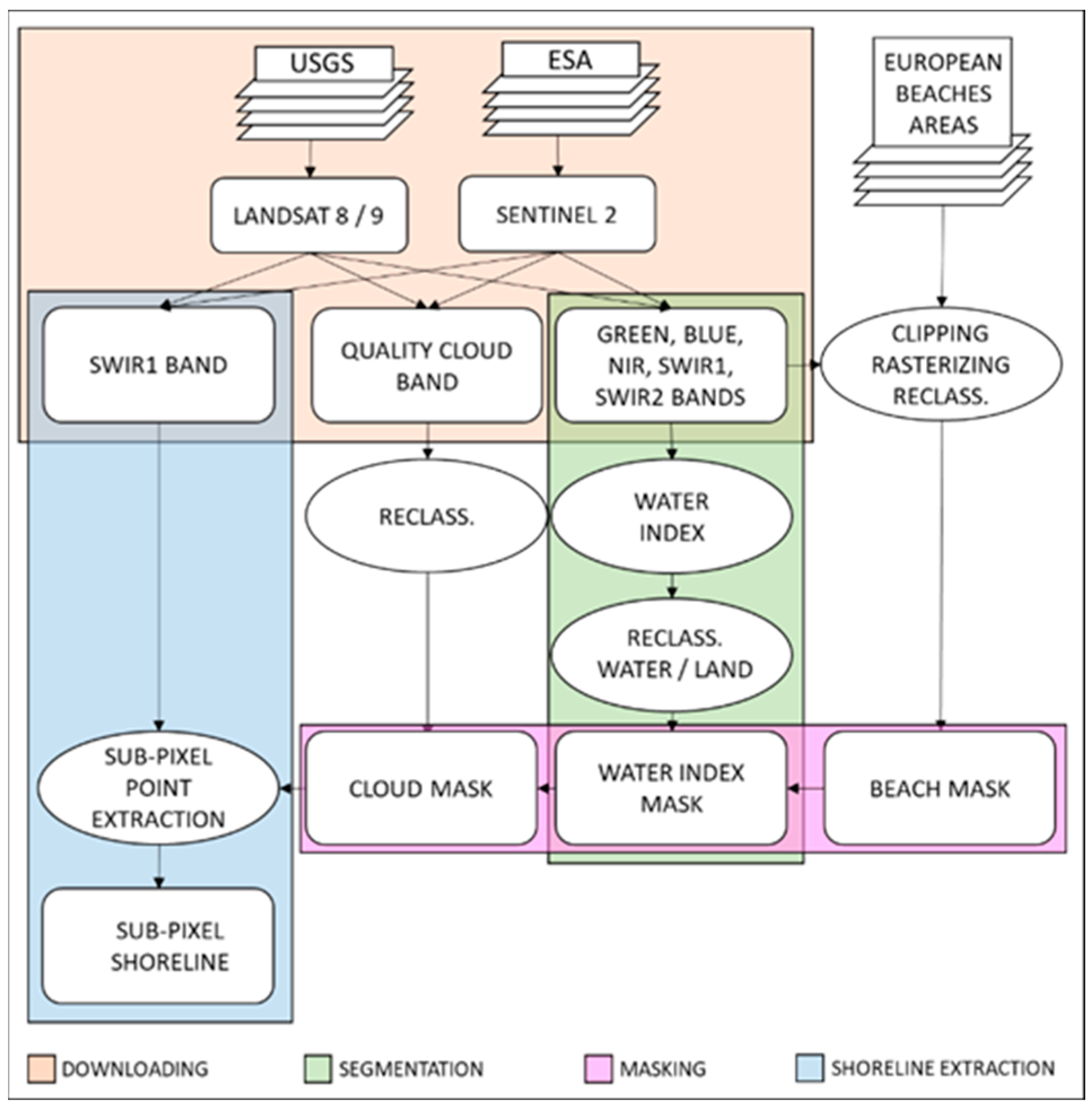
2.2. Workflow

As input, the tool obtains the main information from the optical satellite images (and auxiliary data such as cloud conditions) of the satellites Sentinel-2 (S2), both A and B, and Landsat 8 and 9 (L8 and L9). Both sets of images are freely available from the Copernicus program of the European Space Agency (ESA) and the United States Geological Survey (USGS). The images offer a revisit time of 5 (Sentinel) and 8 (Landsat) days when combined and a spatial resolution of 20 and 30 m for the S2 and Landsat series, respectively. They are retrieved from the official providers: Sentinel images from ESA Copernicus Open Access Hub servers and Landsat images from USGS servers. Before running SAET, it is mandatory to get suitable credentials (user and password) from both providers. In the case of USGS, besides obtaining these credentials, it is also necessary to request access to the machine-to-machine (M2M) application programming interface (API).
The workflow is divided into four main phases (Figure 1):
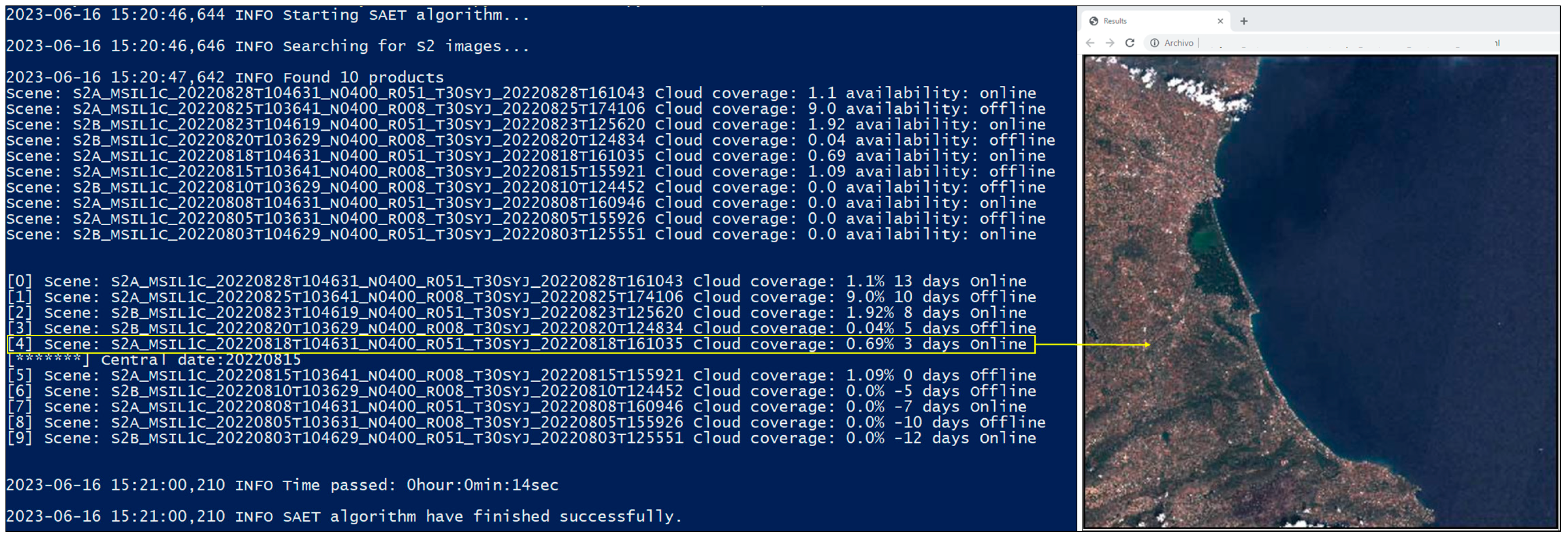
  • Image downloading. SAET is able to analyse entire image scenes, allowing the downloading of S2 and L8–9 images from ESA and USGS servers, respectively. To improve the performance, SAET takes advantage of the capabilities of each server, downloading only the necessary bands when possible. Regarding the ESA server, only the most recently acquired images are immediately available (online mode). On the contrary, it is required to request a specific image to shift from offline to online modes (https://scihub.copernicus.eu/userguide/DataRestoration, accessed on 1 June 2023). This process is relatively fast and does not constitute an important drawback, but the user must be aware of this.
  • Water–land interface segmentation. SAET allows employing different procedures for separating the land and the water coverages. Thus, the images can be segmented by using the clusterisation technique k-means or by combining different bands to create several water indices to obtain a binary water–land mask to determine the position of the shoreline at the pixel level.
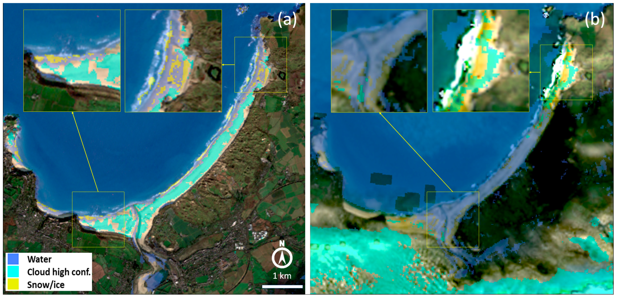
  • Water–land mask refinement. Considering the water-land mask as input, SAET removes all shoreline pixels lying outside beach areas or those that are in pixels classified as clouds. Cloud coverage distribution is obtained from the classification bands associated with both S2 and L8–9 images. On the other hand, beach areas are obtained from the European Coastal Zone dataset, provided by the Copernicus Land Monitoring Service [39].
  • Sub-pixel shoreline extraction. From the pixel-level shoreline obtained in the previous step, SAET computes a new shoreline with sub-pixel accuracy. The core algorithm for sub-pixel shoreline extraction used for SAET takes advantage of the SHOREX system [25,26]. The extraction is carried out by performing a kernel analysis for each pixel classified as shoreline, analysing the gradient variation of the pixel values of the SWIR1 band, as this band has a high contrast between water and land and, at the same time, is less sensitive to disturbing effects, such as those caused by the wave foam, for example. The resulting shorelines can be stored in different geometries and file formats (e.g., polylines or points, SHP or JSON).
It is important to notice that SAET considers some auxiliary data to improve its performance, such as a grid of the satellite imagery scenes and tiles and the beach polygon layer. The overlapping of the area affected by the coastal storm with the scene grids enables to select the scenes of interest and, finally, extract the shoreline comprised within the beach polygons. The beach polygon layer enables to focus the shoreline extraction on specific coastal segments. Although this layer currently includes the beaches along the European coast, it can be easily updated by adding new polygons or modifying the existing ones, allowing the user to adapt SAET to his needs and carry out the analysis in other coastal regions.

2.3. Usage: Running Modes and Main Settings

SAET works in a command-line style by typing the name of the main script followed by the suitable parameters in a terminal window. The parameters can be classified into three categories (Table 1): (i) running modes (only searching, downloading, and processing, only downloading and only processing); (ii) filters (spatial filters by region of interest, ROI, or scenes or attribute filters by type of product); and (iii) advanced parameters, which allow to refine the extraction.
Concerning the running modes, ‘only searching’ is usually the primary option. SAET will retrieve two types of information (Figure 2): an ordered-by-date list of images, which will be displayed directly in the terminal window, and an HTML file containing a preview of the images. The file includes the name of the image, its acquisition date, its cloud cover percentage, the time difference (in days) to the peak of the storm, and whether the image is online or offline (only in the case of S2 images). All this information will help the user decide which are the most suitable pre-storm and post-storm images. Once the images are identified, SAET may be run in the ‘download and processing’ mode, selecting the images of interest. Finally, the user can decide to re-process any image previously downloaded, changing several advanced parameters. In this case, the ‘only processing’ mode avoids downloading the images again. Some examples of SAET command-line sentences are shown in Table 2, where each mode of running involves a specific combination of parameters.

2.4. SAET Customization

In SAET, advanced parameters control the behaviour of several parts involved in the extraction of the shorelines. There are three groups of parameters:
(i)
those (‘wi’ and ‘th’) that let the user choose the band to be segmented (water indices or bands) and the segmentation procedure,
(ii)
those controlling the intensity of the cloud mask, helping to remove shoreline pixels classified as clouds (‘cl’),
(iii)
and finally, those controlling the window size in the kernel analysis (‘ks’).
Although SAET suggests some default values, these parameters can be adapted to the particular features of each type of analysis. Among them, the choice of water index or band and segmentation method is key since they determine the location of the approximate shoreline at the pixel level. Since not all types of combinations perform well on every coastal type, SAET provides three water indices (Table 3) and three thresholding methods, as well as the specific option to threshold the SWIR band with the k-means method. Regarding the water indices, SAET allows the application of the two versions of the Automated Water Extraction Index (AWEI), AWEInsh and AWEIsh [35], together with the MNDWI [31]. As the thresholding values, SAET allows selecting among the value 0, the Otsu method [32], and the multi-Otsu method [40].
The water indices aim to highlight the contrast between land and water. Nevertheless, since all these indices are computed by applying linear combinations of bands, under certain conditions (water turbidity, cirrus, etc.), the value for a specific band is higher or smaller than expected. This may alter the equation, leading to a bad classification of the land and water areas. Thus, in certain cases, as in the Sentinel-2 from 26 February 2022 (Figure 3), the AWEInsh index mistakes water for land, whereas the indices AWEIsh and MNDWI classify water and land reasonably well, with MNDWI being more sensitive to the clouds. However, most of the time the three water indices work reasonably well (as is the case for the Sentinel-2 acquired on 8 April 2017 in the Cornwall region, UK (see Figure 3), even though the AWEInsh gets a better result).
Regarding the influence of the clouds in the extraction, a cloud mask has been introduced within the SAET workflow to reduce the necessity of manual intervention. As pixels classified as clouds cannot be processed, they will be used to mask the shoreline at the pixel level obtained by the water index segmentation. This information can be obtained from the classification bands associated with both S2 and L8–9. Depending on the type of image or its level of processing, the classification may be more or less robust (Table 4).
The process is not completely error-free, and cases of misclassification can be found. In the case of shoreline extraction, if part or the whole beach area is wrongly classified as cloud, SAET will not obtain any result. Therefore, in these cases, it will be necessary to set the parameter ‘cl’ of SAET to the value 0 (low level of cloud severity) to maintain the shoreline that would be removed due to the misclassification of the clouds. When comparing almost-coincident S2 and L9 images affected by clouds and foam (Figure 4), it can be appreciated how the S2 image classifies most of the beach as clouds and the foam as snow/ice, causing the shoreline position to remain undetected. In the case of L9, the presence of clouds is higher, and although the majority of the water/land boundary is correctly identified, the northeast part of the beach is classified as water. This leads to an incorrect definition of the shoreline along the boundary with the vegetated area inland.
As previously stated, when introducing the workflow, the core algorithm of SAET for sub-pixel extraction is based on SHOREX [25,26]. This algorithm takes as input the approximate shoreline at the pixel level obtained from the water index segmentation. Subsequently, it applies a kernel analysis of the SWIR1 band values overlapping the approximate line and identifies the maximum slope in its gradient variation. The values of the SWIR1 band are resampled to increase the spatial resolution and then fitted to a polynomial surface to smooth the transition between adjacent pixels. After that, the Laplacian operator for the polynomial surface is computed. The contour where the Laplacian operator reaches the 0 value will be considered the shoreline with subpixel accuracy. Considering that, it is important to remark that the kernel size is an important parameter conditioning the resulting shoreline position. The larger the kernel, the larger the area to be analysed (3 × 3 kernel represents an area of 60 × 60 m in S2 and 90 × 90 m in L8–9) for subpixel extraction. As a general rule, if the water index segmentation has a good quality and the beach is wide enough, a smaller kernel size can be selected. On the contrary, less confident shorelines at pixel level demand a higher kernel size, but considering that this may bring other problems, for example, in a narrow beach next to a vegetated area, the detected shoreline probably will suffer a landward displacement. To adapt to these different conditions, 3 × 3 and 5 × 5 kernel sizes are available in SAET.

3. Assessment and Example of Application

3.1. Accuracy Assessment of the SDSs against Coincident Reference Lines

The SDSs extracted from SAET on different dates, both from S2 and L8 images, were assessed in order to validate further uses of the extraction tool. For this purpose, the studied sector includes the beaches located between El Saler Beach (València) and the Cape of Cullera (Figure 5), covering a coastal length of about 28 km. This coast is a micro-tidal sandy beach area, showing tidal oscillations below 0.2 m [41] and medium-sized waves, with significant wave heights averaging 0.7 m and a mean wave period reaching 4.2 s [42].
The SDSs were extracted, and their position was planimetrically compared against reference lines obtained on the same day. Two types of information sources were used to define the reference shorelines, covering up to 28 km alongshore (Figure 5). On the one hand, three lines defined at elevation = 0 (14 September 2015; 7 May 2018 and 10 July 2018) were defined alongshore with the DGNSS system by the surveyors of the Spanish General Directorate of Coasts. On the other hand, the reference shoreline was photointerpreted the 26 January 2020 using the VHR image Pléiades 1A, with a 10 min delay with respect to the S2 image.
The SDSs were extracted as points, from which the shortest distance to the reference lines was measured. The total errors (Figure 6) and their averages (Table 5) were calculated for each section. As can be seen, the errors were similar for the four dates, with a very small bias and similar values for the RMSE, which ranged from 2.62 m to 3.79 m. The evaluation has been made using a large number of measurements (more than 7500) on the four dates analysed. The error presents a similar magnitude over the whole area analysed as well as between the different dates, without notable differences between the shorelines extracted from S2 or L8 images.

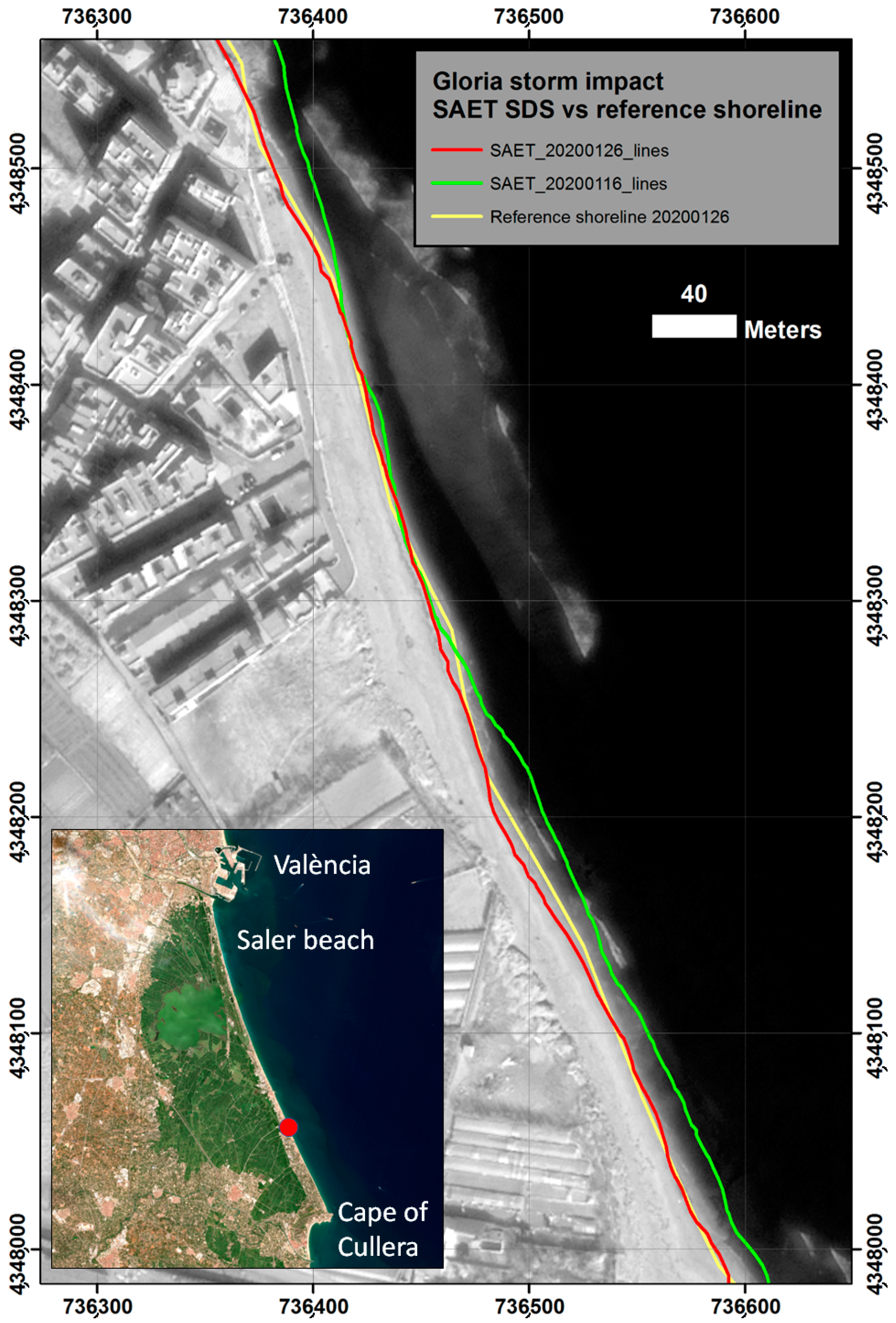
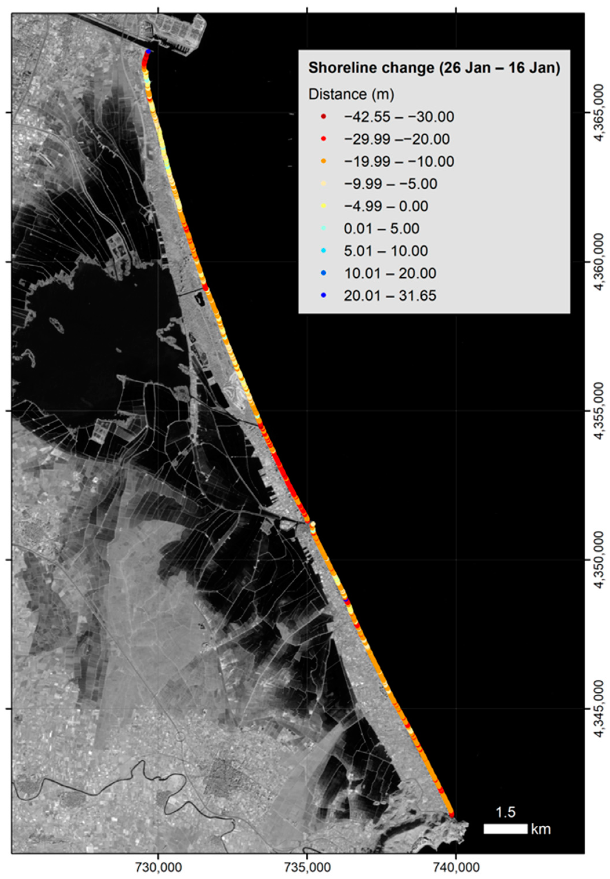
3.2. Application of SAET: Characterising the Shoreline Changes along the Valencian Coast during the Storm Gloria

This section provides an example of the application of SAET for characterising the shoreline changes on the Valencian coast associated with Storm Gloria. This event affected the Spanish Mediterranean coast between 19 and 22 January 2020. The storm peaked on 20 January 2020 (Hs max = 8.09 m, Figure 7), heavily affecting eastern Spain. This storm constitutes a remarkable disruptive event considering its unusually large magnitude and impacts along the Western Mediterranean [42,43,44,45]. As a result, there were very strong impacts of both flooding and erosion on the beaches and coastal dunes.
The first step to analysing the event consists of the selection of suitable satellite images. This selection is based on their coverage and date of acquisition with respect to the storm. Regarding the location, in this example, the whole study site is covered by a single Landsat scene and by a single Sentinel-2 tile (Figure 8). The next step is to search for the closest images before and after the date of the peak of the storm by running SAET in the ‘only searching’ mode. In the event that two products (Landsat and Sentinel-2) coincide on the same date, it would be preferable to use those products with higher spatial resolution.
After running SAET in ‘only searching’ mode (Figure 9), two pre-storm and post-storm Sentinel-2 images were selected (16th and 26th January), according to the criteria of lowest possible cloud coverage and closest to the date of the storm peak (20th January). These two images were used as input to run SAET again, but this time, in mode ‘downloading and processing’, using the default values for the segmentation method (AWEInsh water index with threshold 0). Thus, two Sentinel-2 images were processed, leading to 123 km of extracted shoreline (for each image), a resolution of 1 point every five meters, and a processing time of 10 min (Table 6).
The pre- and post-storm SDSs show an important retreat associated with Storm Gloria along the study area, although with important differences along the coast (Figure 9). The differences are more evident when analysing a much longer stretch, such as the 28 km between the port of Valencia and the Cape of Cullera (Figure 10). Between the two studied dates, 5712 shoreline points were compared, allowing to map the different retreatments along the coast. Furthermore, an average retreat of 13.9 m (±7.4 m) was identified, reaching a maximum retreat of 42.5 m.

4. Discussion

During the past few years, considerable progress has been made in the ability to characterise the evolutionary dynamics of beach spaces over large areas and/or periods at a high level of detail based on the information provided by satellite-derived shorelines (e.g., [7,9,42,46,47]). However, applying these systems over very diverse energetic and environmental conditions has revealed limitations in terms of accuracy, capacity to work over large areas, and dependency on external data and commercial platforms that may jeopardize their public usability in certain countries and/or in the future. Considering the limitations of the existing solutions, SAET is proposed as a new, freely available tool for shoreline extraction in an attempt to overcome them. This solution was developed in association with the ECFAS project, which aims to implement a coastal flooding awareness system at the European scale [37]. SAET will provide the system with SDSs for characterising the shoreline change in response to a storm that may lead to products susceptible to being integrated within the CEMS (as in Figure 11). Furthermore, it constitutes an open-access tool for the analysis of coastal changes. One of the main novelties of SAET compared to other available tools comes from its adaptability to the specific needs imposed by different beach morphologies, oceanographic conditions or the image itself. Some of the examples shown (Figure 3) prove that not all segmentation techniques always work well under all these circumstances. That is why SAET provides several possibilities to use different segmentation options over eligible bands/indices, a possibility that does not exist in any other tool currently available for the definition of SDSs. The NDWI is not included, which is the one proposed by other solutions [21,24,28], but this is so given the serious confusion problems associated with the presence of white water.
Another key advantage of SAET is its efficiency in defining the shoreline position over large areas or coastal segments. As stated before, the extraction of the two SDSs for characterising the impact of Storm Gloria (a total of 123 km of shoreline) took 10 min. Furthermore, the entire process (from image download to SDS retrieval) of extracting a complete Landsat 8 scene (480 km of shoreline) takes only 12 min. This capability contrasts with other open solutions, such as CoastSAT, that require the space to be analysed to be subdivided into small spatial units (coastal segments of less than 10 km). On the other hand, SAET allows the easy reuse of already downloaded images, which substantially shortens the management time since downloading is the most time-consuming phase. This is especially useful in order to carry out a new SDS extraction with different settings.
The evaluation of the SDS shows its good accuracy (2.62–3.79 m RMSE, see Figure 6 and Table 5), comparable to that obtained by SHOREX in similar environments (error of 3.01 and 3.57 m RMSE for S2 and L8 imagery, respectively) as on the sandy beach of Cala Millor, Mallorca [26]. Actually, this fact should not be too surprising since the core algorithmic basis of SAET is the same as that of SHOREX, except for the sub-pixel geometric correction that is not applied in SAET. It is also obvious that the level of accuracy will not necessarily be identical in all environments and oceanographic conditions. If we observe in detail the measured errors along the more than 28 km of beach analysed (Figure 6), it can be seen that for the same date, the bias does not always remain constant. Moreover, it is expected that the SDSs extracted by SAET may be affected by larger biases or errors in the combination of certain morphological and oceanographic conditions. Hagenaars et al. [28] remarked that the accuracy of their method was negatively affected in areas where the beach slope is low, while the results obtained by CoastSat appear considerably conditioned by the run-up and the appearance of intertidal spaces [23]. The occurrence of this type of morphology and oceanographic conditions are therefore expected to affect the SDS positions extracted by SAET. The level of error found in the four tests performed, using both S2 and L8 images, presents very low error magnitudes (the RMSE being clearly lower than 4 m). These values are close to those obtained by SHOREX and suggest that, when considering oceanographic conditions at the moment of image acquisition, SAET could also provide similar errors to those described for SHOREX in mesotidal environments [48] or in energetic coasts such as the Chilean coast [49].
The interpretation of the shoreline position and its changes in the absence of accurate water levels and wave forecasts constitutes a challenge, especially in tidal and/or energetic environments [23]. SAET usage for analysing shoreline changes should be carried out with caution on certain coastal types. In microtidal and low-energetic environments, the SDSs can be interpreted straightforwardly, so any significant change in the position of the shoreline can be interpreted as the beach experiencing erosion or accretion. This is the case of the Mediterranean and Baltic Seas, with a tidal range mainly below 0.5 m (Figure 12) and usually low energetic conditions. On the contrary, in meso/macrotidal and energetic environments, the results provided by the SDSs should be taken with extreme caution. The tidal range and the swash, together with gentle slopes, may translate into important horizontal displacements of the shoreline position. The analysis of the shoreline changes should be carried out with the support of tide levels and wave parameters, together with the beach slope of the studied site, in order to avoid misleading interpretations.
This new solution increases the degree of automation by minimizing manual intervention. This is accomplished by substituting the manual cloud-checking processes followed in SHOREX with cloud probability maps and by applying automatic thresholding techniques, i.e., the AWEInsh index, instead of the manual thresholding supervision proposed by CoastSat and needed when using SHOREX on energetic coasts [48]. Furthermore, the higher degree of automation and efficiency offered by SAET enables the processing of complete S2 tiles or Landsat scenes, thus making it possible to efficiently analyse large geographical areas affected by storms (see Figure 5 and Figure 8 for the application in Valencia).
The example of application along the Valencian coast shows how SAET is able to characterise the shoreline position and the changes that occurred as a response to the outstanding wave conditions that occurred during Storm Gloria along a large coastal segment. The comparison of the position of the SDS obtained before (16 January 2020) and after (26 January 2020) the peak of the storm (Figure 11) allows mapping the shoreline retreat linked to this event along a coastal segment of 28 km length. The extracted SDSs enable the comparison of pre- and post-storm shoreline positions and the quantification of subaerial beach morphological changes over time. In addition to the immediate characterisation of the events, SDSs can be obtained over time, enabling to map the recovery process. Alternatively, its use in local mode enables any user to study change events offline and independently of ECFAS. The SDSs obtained with SAET can be used to monitor not only the morphological changes that occur as a response to coastal storms but also those associated with actions of anthropic origin, such as beach nourishment or the construction of coastal infrastructure. Moreover, while it is designed with the idea of quantifying changes with respect to a given event (such as coastal storms), SAET can also be used to extract large, long-time series of SDSs. Thus, SAET constitutes an advanced tool to complement the existing ones in providing long-term, large-scale, quantitative and homogeneous information. All this will contribute to alleviating the lack of coastal monitoring of sandy beaches necessary for managing this critical zone [50].

5. Conclusions

SAET has been developed as an open-source tool for the efficient definition of SDSs to study the beach response to disruptive events such as coastal storms. It uses EO data from the European Sentinel series (S2 imagery), complemented by the integration of the contributory EO missions Landsat (L8 and L9), which offer a high temporal resolution. SAET is a powerful tool capable of automatically processing complete satellite scenes, enabling the characterisation of the shoreline position along broad beach segments while offering a high level of subpixel accuracy.
SAET is mainly based on the same algorithm employed by SHOREX but with several improvements to increase its efficiency, flexibility and robustness. The modifications include a higher degree of automation by making manual thresholding techniques and cloud-checking processes unnecessary; the omission of the georeferencing process, avoiding the necessity of orthorectified images; and the possibility to easily set different extraction parameters (as the water index and the kernel size, among others) according to the coastal conditions, being completely independent of commercial platforms such as GEE. The shoreline accuracy (assessed along a Mediterranean sandy beach) has the same magnitude as the one obtained by SHOREX under similar conditions, ranging from 2.62 m to 3.79 m RMSE.
SAET appears integrated within the ECFAS project workflow, providing the system with shoreline positions and offering new products to the Copernicus Emergency Management Service (CEMS), such as the study of shoreline changes in response to a storm, as well as the recovery process of a sector. Nevertheless, as an open-source software program, its local mode will allow its use as a completely independent tool for studying the impact and recovery of the beach morphology to any punctual storm event, such as in the case of anthropogenic interventions or even long SDS series.

Author Contributions

Conceptualization, J.P.-V., J.E.P.-P., J.A.-C. and C.C.-R.; methodology, J.P.-V., J.E.P.-P., J.A.-C. and C.C.-R.; software, J.P.-V. and J.A.-C.; validation, J.P.-V., J.E.P.-P., J.A.-C. and C.C.-R.; formal analysis, J.P.-V., J.E.P.-P., J.A.-C. and C.C.-R.; investigation, J.P.-V., J.E.P.-P., J.A.-C. and C.C.-R.; resources, J.E.P.-P. and C.C.-R.; data curation, J.P.-V., J.E.P.-P., J.A.-C. and C.C.-R.; writing—original draft preparation, C.C.-R.; writing—review and editing, J.P.-V., J.E.P.-P., J.A.-C. and C.C.-R.; visualization, J.P.-V., J.E.P.-P. and C.C.-R.; supervision, J.E.P.-P.; project administration, J.E.P.-P. and C.C.-R.; funding acquisition, J.E.P.-P. and C.C.-R. All authors have read and agreed to the published version of the manuscript.

Funding

The ECFAS (European Coastal Flood Awareness System) project (https://www.ecfas.eu/) has received funding from the EU H2020 research and innovation programme under Grant Agreement No. 101004211. This research is also supported by the projects MONOBESAT (PID2019-111435RB-I00) funded by the Spanish Ministry of Science, Innovation and Universities, and the Margarita Salas contract within the Re-qualification programme by the Ministry of Universities financed by the European Union–NextGenerationEU and the grant Primeros Proyectos de Investigación (PAID-06-22), Vicerrectorado de Investigación de la Universitat Politècnica de València (UPV) associated with the corresponding author.

Data Availability Statement

The software is freely available at https://doi.org/10.5281/zenodo.7488654 (accessed on 1 June 2023).

Acknowledgments

Authors acknowledge the Spanish General Directorate of Coasts in Valencia for providing the DGNSS surveys.

Conflicts of Interest

The authors declare no conflict of interest.

References

  1. de Schipper, M.A.; Ludka, B.C.; Raubenheimer, B.; Luijendijk, A.P.; Schlacher, T. Beach nourishment has complex implications for the future of sandy shores. Nat. Rev. Earth Environ. 2021, 2, 70–84. [Google Scholar] [CrossRef]
  2. Castelle, B.; Marieu, V.; Bujan, S. Alongshore-variable beach and dune changes on the timescales from days (storms) to decades along the rip-dominated beaches of the Gironde Coast, SW France. J. Coast. Res. 2019, 88, 157–171. [Google Scholar] [CrossRef]
  3. IPCC. Intergovernmental Panel on Climate Change Climate Change 2014: Synthesis Report. In Contribution of Working Groups I, II and III to the Fifth Assessment Report of the Intergovernmental Panel on Climate Change; Meyer, R.K., Pachauri, L.A., Eds.; IPCC: Geneva, Switzerland, 2014; pp. 1–5. [Google Scholar]
  4. Schlacher, T.A.; Schoeman, D.S.; Dugan, J.; Lastra, M.; Jones, A.; Scapini, F.; McLachlan, A. Sandy beach ecosystems: Key features, sampling issues, management challenges and climate change impacts. Mar. Ecol. 2008, 29, 70–90. [Google Scholar] [CrossRef]
  5. Calafat, F.M.; Wahl, T.; Tadesse, M.G.; Sparrow, S.N. Trends in Europe storm surge extremes match the rate of sea-level rise. Nature 2022, 603, 841–845. [Google Scholar] [CrossRef]
  6. Ballesteros, C.; Jiménez, J.A.; Valdemoro, H.I.; Bosom, E. Erosion consequences on beach functions along the Maresme coast (NW Mediterranean, Spain). Nat. Hazards 2018, 90, 173–195. [Google Scholar] [CrossRef] [Green Version]
  7. Cabezas-Rabadán, C.; Pardo-Pascual, J.E.; Almonacid-Caballer, J.; Rodilla, M. Detecting problematic beach widths for the recreational function along the Gulf of Valencia (Spain) from Landsat 8 subpixel shorelines. Appl. Geogr. 2019, 110, 102047. [Google Scholar] [CrossRef]
  8. Jiménez, J.A.; Gracia, V.; Valdemoro, H.I.; Mendoza, E.T.; Sánchez-Arcilla, A. Managing erosion-induced problems in NW Mediterranean urban beaches. Ocean. Coast. Manag. 2011, 54, 907–918. [Google Scholar] [CrossRef]
  9. Cabezas-Rabadán, C.; Pardo-Pascual, J.E.; Palomar-Vázquez, J.; Fernández-Sarría, A. Characterizing beach changes using high-frequency Sentinel-2 derived shorelines on the Valencian coast (Spanish Mediterranean). Sci. Total Environ. 2019, 691, 216–231. [Google Scholar] [CrossRef]
  10. Melet, A.; Buontempo, C.; Mattiuzzi, M.; Salamon, P.; Bahurel, P.; Breyiannis, G.; Burgess, S.; Crosnier, L.; Le Traon, P.; Mentaschi, L.; et al. European Copernicus Services to Inform on Sea-Level Rise Adaptation: Current Status and Perspectives. Front. Mar. Sci. 2021, 8, 1142. [Google Scholar] [CrossRef]
  11. Darwish, K.; Smith, S. Landsat-Based Assessment of Morphological Changes along the Sinai Mediterranean Coast between 1990 and 2020. Remote Sens. 2023, 15, 1392. [Google Scholar] [CrossRef]
  12. Muzirafuti, A.; Crupi, A.; Lanza, S.; Barreca, G.; Randazzo, G. Shallow water bathymetry by satellite image: A case study on the coast of San Vito Lo Capo Peninsula, Northwestern Sicily, Italy. In Proceedings of the IMEKO TC-19 International Workshop on Metrology for the Sea, Genoa, Italy, 3–5 October 2019. [Google Scholar]
  13. Viaña-Borja, S.P.; Fernández-Mora, A.; Stumpf, R.P.; Navarro, G.; Caballero, I. Semi-automated bathymetry using Sentinel-2 for coastal monitoring in the Western Mediterranean. Int. J. Appl. Earth Obs. Geoinf. 2023, 120, 103328. [Google Scholar] [CrossRef]
  14. Li, J.; Roy, D.P. A global analysis of Sentinel-2A, Sentinel-2B and Landsat 8 data revisit intervals and implications for terrestrial monitoring. Remote Sens. 2017, 9, 902. [Google Scholar] [CrossRef] [Green Version]
  15. Coco, G.; Senechal, N.; Rejas, A.; Bryan, K.R.; Capo, S.; Parisot, J.P.; Brown, J.A.; MacMahan, J.H. Beach response to a sequence of extreme storms. Geomorphology 2014, 204, 493–501. [Google Scholar] [CrossRef] [Green Version]
  16. Bishop-Taylor, R.; Sagar, S.; Lymburner, L.; Alam, I.; Sixsmith, J. Sub-pixel waterline extraction: Characterising accuracy and sensitivity to indices and spectra. Remote Sens. 2019, 11, 2984. [Google Scholar] [CrossRef] [Green Version]
  17. Chen, W.W.; Chang, H.K. Estimation of shoreline position and change from satellite images considering tidal variation. Estuarine. Coast. Shelf Sci. 2009, 84, 54–60. [Google Scholar] [CrossRef]
  18. Foody, G.M.; Muslim, A.M.; Atkinson, P.M. Super-resolution mapping of the waterline from remotely sensed data. Int. J. Remote Sens. 2005, 26, 5381–5392. [Google Scholar] [CrossRef]
  19. Gens, R. Remote sensing of coastlines: Detection, extraction and monitoring. Int. J. Remote Sens. 2010, 31, 1819–1836. [Google Scholar] [CrossRef]
  20. Ghosh, M.K.; Kumar, L.; Roy, C. Monitoring the coastline change of Hatiya Island in Bangladesh using remote sensing techniques. ISPRS J. Photogramm. Remote Sens. 2015, 101, 137–144. [Google Scholar] [CrossRef]
  21. Luijendijk, A.; Hagenaars, G.; Ranasinghe, R.; Baart, F.; Donchyts, G.; Aarninkhof, S. The State of the World’s Beaches. Sci. Rep. 2018, 8, 6641. [Google Scholar] [CrossRef]
  22. Wang, C.; Zhang, J.; Ma, Y. Coastline interpretation from multispectral remote sensing images using an association rule algorithm. Int. J. Remote Sens. 2010, 31, 6409–6423. [Google Scholar] [CrossRef]
  23. Castelle, B.; Masselink, G.; Scott, T.; Stokes, C.; Konstantinou, A.; Marieu, V.; Bujan, S. Satellite-derived shoreline detection at a high-energy meso-macrotidal beach. Geomorphology 2021, 383, 107707. [Google Scholar] [CrossRef]
  24. Almeida, L.P.; de Oliveira, I.E.; Lyra, R.; Dazzi RL, S.; Martins, V.G.; da Fontoura Klein, A.H. Coastal analyst system from space imagery engine (CASSIE): Shoreline management module. Environ. Model. Softw. 2021, 140, 105033. [Google Scholar] [CrossRef]
  25. Cabezas-Rabadán, C.; Pardo-Pascual, J.E.; Palomar-Vázquez, J. Characterizing the Relationship between the Sediment Grain Size and the Shoreline Variability Defined from Sentinel-2 Derived Shorelines. Remote Sens. 2021, 13, 2829. [Google Scholar] [CrossRef]
  26. Sánchez-García, E.; Palomar-Vázquez, J.M.; Pardo-Pascual, J.E.; Almonacid-Caballer, J.; Cabezas-Rabadán, C.; Gómez-Pujol, L. An efficient protocol for accurate and massive shoreline definition from mid-resolution satellite imagery. Coast. Eng. 2020, 160, 103732. [Google Scholar] [CrossRef]
  27. Vos, K.; Splinter, K.D.; Harley, M.D.; Simmons, J.A.; Turner, I.L. CoastSat: A Google Earth Engine-enabled Python toolkit to extract shorelines from publicly available satellite imagery. Environ. Model. Softw. 2019, 122, 104528. [Google Scholar] [CrossRef]
  28. Hagenaars, G.; de Vries, S.; Luijendijk, A.P.; de Boer, W.P.; Reniers, A.J. On the accuracy of automated shoreline detection derived from satellite imagery: A case study of the sand motor mega-scale nourishment. Coast. Eng. 2018, 133, 113–125. [Google Scholar] [CrossRef]
  29. Gao, B.C. NDWI—A normalized difference water index for remote sensing of vegetation liquid water from space. Remote Sens. Environ. 1996, 58, 257–266. [Google Scholar] [CrossRef]
  30. Pardo-Pascual, J.E.; Sánchez-García, E.; Almonacid-Caballer, J.; Palomar-Vázquez, J.M.; Priego De Los Santos, E.; Fernández-Sarría, A.; Balaguer-Beser, Á. Assessing the accuracy of automatically extracted shorelines on microtidal beaches from Landsat 7, Landsat 8 and Sentinel-2 imagery. Remote Sens. 2018, 10, 326. [Google Scholar] [CrossRef] [Green Version]
  31. Xu, H. Modification of normalised difference water index (NDWI) to enhance open water features in remotely sensed imagery. Int. J. Remote Sens. 2006, 27, 3025–3033. [Google Scholar] [CrossRef]
  32. Otsu, N. A threshold selection method from gray-level histogram. IEEE Trans. Syst. Man Cybemetic 1979, 9, 62–66. [Google Scholar] [CrossRef] [Green Version]
  33. Cipolletti, M.P.; Delrieux, C.A.; Perillo, G.M.; Piccolo, M.C. Superresolution border segmentation and measurement in remote sensing images. Comput. Geosci. 2012, 40, 87–96. [Google Scholar] [CrossRef]
  34. Lorensen, W.E.; Cline, H.E. Marching cubes: A high resolution 3D surface construction algorithm. ACM Siggr. Comput. Graph. 1987, 21, 163–169. [Google Scholar] [CrossRef]
  35. Feyisa, G.L.; Meilby, H.; Fensholt, R.; Proud, S.R. Automated Water Extraction Index: A new technique for surface water mapping using Landsat imagery. Remote Sens. Environ. 2014, 140, 23–35. [Google Scholar] [CrossRef]
  36. Pardo-Pascual, J.E.; Almonacid-Caballer, J.; Ruiz, L.A.; Palomar-Vázquez, J. Automatic extraction of shorelines from Landsat TM and ETM+ multi-temporal images with subpixel precision. Remote Sens. Environ. 2012, 123, 1–11. [Google Scholar] [CrossRef] [Green Version]
  37. Irazoqui-Apecechea, M.; Melet, A.; Armaroli, C. Towards a pan-European coastal flood awareness system: Skill of extreme sea-level forecasts from the Copernicus Marine Service. Front. Mar. Sci. 2023, 9, 1091844. [Google Scholar] [CrossRef]
  38. Almonacid-Caballer, J.; Pardo-Pascual, J.E.; Ruiz, L.A. Evaluating fourier cross-correlation sub-pixel registration in landsat images. Remote Sens. 2017, 9, 1051. [Google Scholar] [CrossRef] [Green Version]
  39. CLMS. Copernicus Land Monitoring Service. European Coastal Zone. 2018. Available online: https://land.copernicus.eu/local/coastal-zones/coastal-zones-2018 (accessed on 1 September 2022).
  40. Liao, P.-S.; Chen, T.-S.; Chung, P.-C. A fast algorithm for multilevel thresholding. J. Inf. Sci. Eng. 2001, 17, 713–727. [Google Scholar] [CrossRef]
  41. REDMAR—Red de Mareógrafos de Puertos del Estado. Resumen de los Parámetros Relacionados Con el Nivel del Mar y la Marea que Afectan a las Condiciones de Diseño y Explotación Portuaria. Puerto de Valencia. Dirección Técnica Puertos del Estado. 2019. Available online: https://bancodatos.puertos.es/BD/informes/globales/GLOB_2_3_3651.pdf (accessed on 29 September 2022).
  42. Pardo-Pascual, J.E.; Palomar-Vázquez, J.; Cabezas-Rabadán, C. Estudio de los cambios de posición de la línea de costa en las playas del segmento València-Cullera (1984–2020) a partir de imágenes de satélite de resolución media de libre acceso. Cuad. De Geogr. 2022, 108, 79–104. [Google Scholar] [CrossRef]
  43. Amores, A.; Marcos, M.; Carrió, D.S.; Gómez-Pujol, L. Coastal impacts of Storm Gloria (January 2020) over the north-western Mediterranean. Nat. Hazards Earth Syst. Sci. 2020, 20, 1955–1968. [Google Scholar] [CrossRef]
  44. Berdalet, E.; Marrasé, C.; Pelegrí, J.L. Resumen sobre la Formación y Consecuencias de la Borrasca Gloria (19–24 Enero 2020); CSIC—Instituto de Ciencias del Mar (ICM): Barcelona, Spain, 2020. [Google Scholar] [CrossRef]
  45. de Alfonso, M.; Lin-Ye, J.; García-Valdecasas, J.M.; Pérez-Rubio, S.; Luna, M.Y.; Santos-Muñoz, D.; Ruiz, M.I.; Pérez-Gómez, B.; Álvarez-Fanjul, E. Storm Gloria: Sea state evolution based on in situ measurements and modeled data and its impact on extreme values. Front. Mar. Sci. 2021, 8, 270. [Google Scholar] [CrossRef]
  46. Bishop-Taylor, R.; Nanson, R.; Sagar, S.; Lymburner, L. Mapping Australia’s dynamic coastline at mean sea level using three decades of Landsat imagery. Remote Sens. Environ. 2021, 267, 112734. [Google Scholar] [CrossRef]
  47. Vos, K.; Harley, M.D.; Splinter, K.D.; Simmons, J.A.; Turner, I.L. Sub-annual to multi-decadal shoreline variability from publicly available satellite imagery. Coast. Eng. 2019, 150, 160–174. [Google Scholar] [CrossRef]
  48. Cabezas-Rabadan, C.; Pardo-Pascual, J.E.; Palomar-Vazquez, J.; Ferreira, O.; Costas, S. Satellite derived shorelines at an exposed meso-tidal beach. J. Coast. Res. 2020, 95, 1027–1031. [Google Scholar] [CrossRef]
  49. Sánchez-García, E.; Briceño, I.; Palomar-Vázquez, J.; Pardo-Pascual, J.E.; Cabezas-Rabadán, C.; Balaguer-Beser, Á. Beach monitoring project on central Chile. In Proceedings of the 5ª Conferência sobre Morfodinâmica Estuarina e Costeira (MEC2019), Lisboa, Portugal, 24–26 May 2019; pp. 49–50. [Google Scholar]
  50. Splinter, K.D.; Coco, G. Challenges and Opportunities in Coastal Shoreline Prediction. Front. Mar. Sci. 2021, 8. [Google Scholar] [CrossRef]
Figure 1. SAET workflow.
Remotesensing 15 03198 g001
Figure 2. Example of the results obtained in the searching mode (S2 images). On the left, the first list shows the found images and their availability, while the second list is an ordered-by-date list including the central date and showing only the images that are available (online). On the right, the HTML file displays an overview of the found images. The yellow box highlights the information for the closest image to the analysed date. The parameters to obtain this result are the following (see Table 1): --rm=os --fp=NONE --sd=20220801 --cd=20220815 --ed=20220830 --mc=10 --lp=NONE --ll=NONE --sp=S2MSI1C --sl=30SYJ.
Remotesensing 15 03198 g002
Figure 3. For the coast of Cornwall (U.K.), the four first images show (a) the RGB Sentinel-2, the indices (b) AWEInsh, (c) AWEIsh, and (d) MNDWI using the 0 threshold for the date 26 February 2022. The next four images show (e) the Sentinel-2 and the indices in the same order (fh) for the date 8 April 2017.
Remotesensing 15 03198 g003
Figure 4. S2 (a) and L9 (b) images of St. Ives Bay (Cornwall, U.K.) were acquired the same day with only 10 min of difference. The classification, mainly focused on water and clouds (high confidence) classes, shows several problems of misclassification.
Remotesensing 15 03198 g004
Figure 5. Location map of the study area between Valencia Port and the Cape of Cullera (Spain). The sections considered in the shoreline assessment appeared in black (7 May 2018), green (14 September 2015), yellow (10 July 2018) and blue (26 January 2020). The SIMAR point was employed for defining the oceanographic data at the moment of the assessment. Source: EO Browser, https://apps.sentinel-hub.com/eo-browser/ (accessed on 10 April 2023), Sinergise Ltd. (Ljubljana, Slovenia).
Remotesensing 15 03198 g005
Figure 6. Errors of the SDSs along the study site. Positive values represent a seaward bias, while negative values indicate a landward bias.
Remotesensing 15 03198 g006
Figure 7. Significant wave height (m) and availability of satellite imagery during the occurrence of Storm Gloria (January 2020). Data from the SIMAR station 2,081,111 (0.25°O, 39.25°N) by the Spanish Ports Authority (https://www.puertos.es/es-es/oceanografia/Paginas/portus.aspx, accessed on 10 April 2023). The pre-storm and post-storm images employed for the shoreline extraction are shown in green and red colour respectively. Likewise, coinciding with the post-storm image, the very high-resolution image used for the accuracy assessment also appears.
Remotesensing 15 03198 g007
Figure 8. The study area (in red) is covered by both a Sentinel-2 tile (30SYJ, in blue) and a Landsat scene (198,033, in purple). The choice of one or the other product will depend on which images are closest to the peak of the storm.
Remotesensing 15 03198 g008
Figure 9. Ordered-by-date list of the available satellite images. This list offers some information about each image, such as the identifier, the cloud coverage percentage, and the difference in days with respect to the peak of the storm. In this example, Sentinel-2 numbers 0 (26 January) and 1 (16 January) are selected to run SAET in the ‘downloading and processing’ mode.
Remotesensing 15 03198 g009
Figure 10. Detail of the extracted shorelines associated with Storm Gloria. The pre-storm (in green) and post-storm (in red) SDSs are displayed together with the reference line from the VHR image (in yellow). Coordinate system: WGS84/UTM 30N. Background image: Pléiades-1A © CNES (2020), distributed by Airbus DS, provided under COPERNICUS by the European Union and ESA, all rights reserved.
Remotesensing 15 03198 g010
Figure 11. Shoreline change measured with SAET as response to Storm Gloria along 28 km of the Valencian coast. Coordinate system: WGS84/UTM 30N. Background image: Pléiades-1A © CNES (2020), distributed by Airbus DS, provided under COPERNICUS by the European Union and ESA, all rights reserved.
Remotesensing 15 03198 g011
Figure 12. Tidal range along the coast of Europe. Data obtained from the Global Tidal Range dataset computed by ESRI (https://www.arcgis.com/home/item.html?id=d5354dea41b14f0689860bf4b2cf5e8a, accessed on 2 June 2023) using the FES2014 tide model produced by Noveltis, Legos and CLS and distributed by Aviso+, with support from Cnes (https://www.aviso.altimetry.fr/, accessed on 2 June 2023).
Remotesensing 15 03198 g012
Table 1. SAET settings.
ParameterTypeDescription
rmRunning modeRun mode ‘os’ (only searching) is used to search images, ‘dp’ for downloading and processing images, ‘od’ for downloading images without processing, and ‘op’ for processing or re-processing previous downloaded images using different advanced parameters.
fp (footprint)FilterROI for scene searching. This parameter has three ways to be used:
-Path to the ROI file (in.json format).
-Bounding box in latitude and longitude coordinates.
-The value NONE for this parameter will deactivate the spatial filter and the user will be able to activate the filter by scenes (parameters--ll and-sl).
sd (start date)FilterStart date for searching scenes.
cd (central date)FilterCentral date for searching the scenes. It is assumed to be the central date of the storm.
ed (end date)FilterEnd date for searching scenes.
mc (maxim cloud coverage)FilterMaximum percentage of cloud coverage in the scene.
lp (Landsat products)FilterProduct type for L8-9 scenes. By default, SAET uses the Collection 1 to search L8 images, but it also can search L8-9 from Collection 2 at levels 1 and 2.
ll (list of Landsat scenes)FilterScene list identifiers for Landsat images. This parameter is used only if the spatial filter by ROI is deactivated.
sp (Sentinel-2 product)FilterProduct type for S2 tiles. By default, SAET uses Sentinel-2 at level 1C, but the user also can search images of level 2A.
sl (list of Sentinel-2 tiles)FilterScene list identifiers for S2. This parameter is used only if the spatial filter by ROI is deactivated.
of (output folder)AdvancedOutput data folder. By default, this folder will be located in the SAET installation folder but can be defined by the user
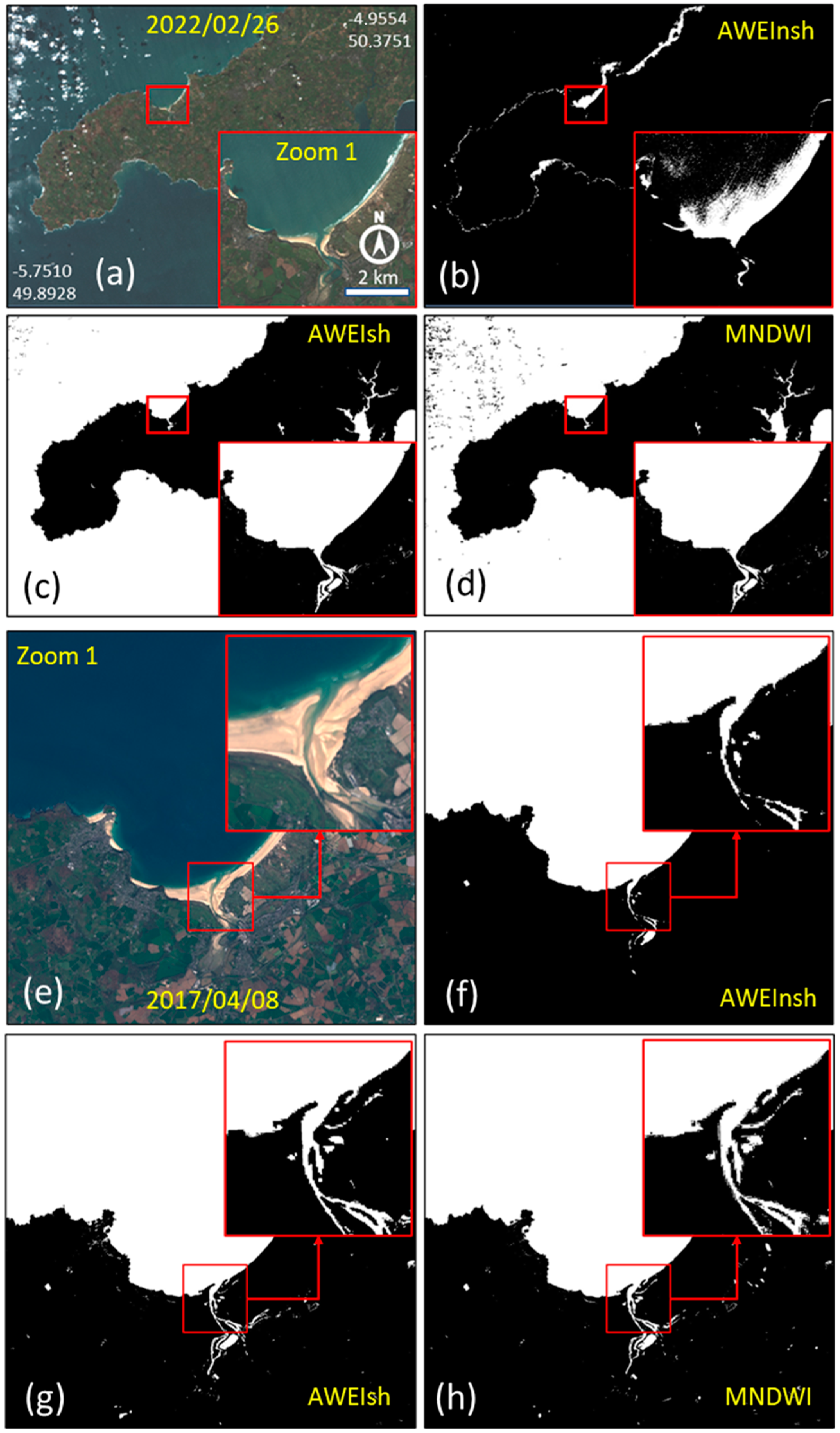
wi (water index)AdvancedWater index type. SAET supports the indices AWEINSH, AWEISH and MNDWI.
th (thresholding/segmentation method)AdvancedThreshold method to obtain the water-land mask from the water index. SAET supports four methods: standard 0 value, Otsu bimodal, and Otsu multimodal with three classes and the clustering method k-means (only to SWIR band).
mm (morphological method)AdvancedMorphological method. Used to obtain the shoreline at pixel level from the water-land mask. SAET can apply two methods: erosion and dilation.
cl (cloud masking severity)AdvancedCloud masking severity. This parameter controls the type of clouds considered to refine the initial water-land mask. Three levels may be defined: low (SAET does not use any cloud mask Value 0), medium (only opaque clouds are used. Value 1), and high (opaque clouds, cirrus, and cloud shadows are used. Value 2).
ks (kernel size)AdvancedKernel size. Advanced users can control the size of the kernel analysed when the subpixel extraction takes place, choosing between 3 and 5 pixels.
np (number of products)FilterThe number of products (identifiers). List of products to be processed in both ‘dp’ and ‘op’ modes. This list makes reference to the products found by SAET in the searching mode. This parameter supports three different formats: list of identifiers, range of identifiers, or all identifiers.
Table 2. Examples of command-line sentences to run SAET.
ModeCommand-Line SentenceDescription
Only searchingsaet_run.py --rm=os --fp=NONE --sd=20220801 --cd=20220815 --ed=20220830 --mc=10 --lp=NONE --ll=NONE --sp=S2MSI1C --sl=30SYJSearching for Sentinel-2 (level 1C) images from 1 August to 30 August 2020, belonging to the tile ‘30SYJ’ and with a cloud coverage of less than 10%
Downloading and processingsaet_run.py --rm=dp --fp=NONE --sd=20220801 --cd=20220815 --ed=20220830 --mc=10 --lp=NONE --ll=NONE --sp=S2MSI1C --sl=30SYJ --np=3,4,6,8 Downloading and processing Sentinel-2 (level 1C) images from 1 August to 30 August 2020, belonging to the tile ‘30 SYJ’ and with a cloud coverage of less than 10%. The ‘np’ parameter indicates which images, from the list of found images, will be processed (in this case, images 3, 4, 6, and 8).
Only processingsaet_run.py --rm=op --wi=aweish --cl=2Processing of the images stored in the data folder, using different values to the default values for some advanced parameters: water index (--wi. Default value: ‘aweinsh’) and cloud masking severity (--cl. Default value: 0 (without mask)).
Table 3. Water indices applied by SAET. Positive values refer to the water, while negative values refer to the land.
Water IndexExpression
AWEInsh 4 g r e e n S W I R 1 0.25 N I R + 2.75 S W I R 2
AWEIsh b l u e + 2.5 g r e e n 1.5 N I R + S W I R 1 0.25 S W I R 2
MNDWI g r e e n S W I R 1 g r e e n + S W I R 1
Table 4. Cloud classification bands for S2 and L8–9 imagery and their different characteristics. TOA indicates top-of atmosphere processing, and SR refers to the surface reflectance.
Image TypeImage Level of ProcessingBandResolution (m)Description
S21C (TOA)QA6060Classification: opaque clouds, cirrus, and no clouds.
Source: https://sentinel.esa.int/web/sentinel/technical-guides/sentinel-2-msi/level-1c/cloud-masks (accessed on 1 June 2023)
S22A (SR)SCL20Classification: low, medium, or high cloud probability; presence of cirrus; cloud shadows. Source: https://sentinels.copernicus.eu/web/sentinel/technical-guides/sentinel-2-msi/level-2a/algorithm-overview (accessed on 18 June 2023)
L8–91 (TOA) and 2 (SR)QA_PIXEL30Classification: based on levels of confidence (low, medium, high) for clouds, cirrus, and cloud shadows.
Source: https://www.usgs.gov/landsat-missions/landsat-collection-2-quality-assessment-bands (accessed on accessed on 1 June 2023)
Table 5. Shorelines extracted from Landsat 8 and Sentinel-2 imagery, data employed for defining the reference lines to compare them with, and the oceanographic conditions for the moments of the image acquisition. The VHR image is a Pléiades 1A and was obtained from ESA Data Warehouse (IMG_PHR1A__PMS_202001261050033_ORT_4779958101-001_R1C). The average errors for each SDS/date appear expressed as bias, σ and RMSE, all of them in m.
Date (dd/mm/yy)Satellite ImageReference DataSea Level (m)Hs (m)Tp (s)No. DataBias (m)Standard Deviation (m)RMSE (m)
26 January 2020S2Pléiades0.2200.528.2750380.033.793.79
10 July 2018L8DGNSS0.0960.125.1313670.122.622.62
7 May 2018L8DGNSS0.0850.225.56384−1.023.613.75
14 September 2015S2DGNSS0.1750.322.43885−0.112.752.75
Table 6. Settings of SAET.
SAET ModeCommand LineDescription
Only searchingsaet_run.py --rm=os --fp=NONE --sd=20200110 --cd=20200120 --ed=20200130 --mc=10 --lp=NONE --ll=NONE --sp=S2MSI1C --sl=30SYJSearching for level 1C Sentinel-2 images belonging to the tile ‘30SYJ’, with a cloud cover of less than 10%, and that was acquired between 10 January and 30 January 2020.
Downloading and processingsaet_run.py --rm=dp --fp=NONE --sd=20200110 --cd=20200120 --ed=20200130 --mc=10 --lp=NONE --ll=NONE --sp=S2MSI1C --sl=30SYJ --np=0,1Downloading and processing images [0] and [1]. These images correspond with the position of each selected image in the list obtained when running SAET in the ‘only searching’ mode.
Disclaimer/Publisher’s Note: The statements, opinions and data contained in all publications are solely those of the individual author(s) and contributor(s) and not of MDPI and/or the editor(s). MDPI and/or the editor(s) disclaim responsibility for any injury to people or property resulting from any ideas, methods, instructions or products referred to in the content.

