A High-Performance Automated Large-Area Land Cover Mapping Framework

Abstract

Land cover mapping plays a pivotal role in global resource monitoring, sustainable development research, and effective management. However, the complexity of the mapping process, coupled with significant computational and data storage requirements, often leads to delays between data processing and product publication, thereby bringing challenges to creating multi-timesteps large-area products for monitoring dynamic land cover. Therefore, improving the efficiency of each stage in land cover mapping and automating the mapping process is currently an urgent issue to be addressed. This study proposes a high-performance automated large-area land cover mapping framework (HALF). By leveraging Docker and workflow technologies, the HALF effectively tackles model heterogeneity in complex land cover mapping processes, thereby simplifying model deployment and achieving a high degree of decoupling between production models. It optimizes key processes by incorporating high-performance computing techniques. To validate these methods, this study utilized Landsat imagery data and extracted samples using GLC_FCS and FROM_GLC, all of which were acquired at a spatial resolution of 30 m. Several 10° × 10° regions were chosen globally to illustrate the viability of generating large-area land cover using the HALF. In the sample collection phase, the HALF introduced an automated method for generating samples, which overlayed multiple prior products to generate a substantial number of samples, thus saving valuable manpower resources. Additionally, the HALF utilized high-performance computing technology to enhance the efficiency of the sample–image matching phase, thereby achieving a speed that was ten times faster than traditional matching methods. In the mapping stage, the HALF employed adaptive classification models to train the data in each region separately. Moreover, to address the challenge of handling a large number of classification results in a large area, the HALF utilized a parallel mosaicking method for classification results based on the concept of grid division, and the average processing time for a single image was approximately 6.5 s.

1. Introduction

Global land cover (GLC) plays a critical role in global resource monitoring and sustainable development research, as it provides vital insights into ecological diversity, carbon cycling, and human–environment relationships [1,2,3]. In recent years, with the rapid development of remote sensing technology, land cover classification based on remote sensing images has become the mainstream method for modern land cover mapping.

Unlike satellite images, which are usually obtained in near-real-time, GLC products are typically associated with substantial lag times between the processing of images and the release of data [4]. The shortest production cycle of a GLC product is usually one year, and seasonal or monthly datasets are relatively rare [5]. In addition, the higher the product resolution is, the longer the production cycle. Currently, there are many GLC products that are updated annually, such as the Moderate Resolution Imaging Spectroradiometer (MODIS) Land Cover Type product (MCD12Q1), each with a resolution of 500 m provided by National Aeronautics and Space Administration (NASA) from 2001 to present [6]; the Climate Change Initiative (CCI) program of the European Space Agency (ESA) provides a 300 m dataset (1992–2018), and the Copernicus Global Land Service (CGLS) [7] provides a 100 m dataset for land cover. Chen et al. [8] produced the GlobeLand30 with a resolution of 30 m from Landsat and China’s HJ-1 satellite images for 2000 and 2010. The latest version was launched for updating in 2017 and was officially released in 2020. GLC with yearly or even higher intervals limits the monitoring capability of land cover dynamic changes. Until 2021, the ESA provided the WorldCover [9], a GLC product based on Sentinel data, with a resolution of 10m, with the potential to be produced within approximately 3 months of the acquisition of the last image. In 2022, Google released the Dynamic World [4], which is a near real-time LC product. It utilizes cloud computing platforms to acquire and predict the classification probabilities of Sentinel images in real-time. This marks a new era for the fast mapping and updating of GLC within the realm of big data, and an increasing number of researchers have started conducting related studies. Hence, improving the computational efficiency of various stages in land cover mapping using big data and automating the mapping process currently have become the key issues that need to be addressed. Larger area, higher resolution, and faster update frequency have exponentially increased the amount of data, thereby posing new challenges for storage and computing power. At the same time, the land cover mapping process is complex, and each stage depends on different models. The process of improving the efficiency of each link in land cover mapping, systematizing and standardizing the mapping process, and achieving the automated mapping of large-area land cover has gradually become one of the key issues.

As supervised classification algorithms are widely applied in remote sensing image classification, obtaining a large number of accurate samples is crucial for training classification models. Sample collection is considered the most time-consuming and labor-intensive process in producing GLC [10]. Existing methods for extracting classification samples still rely primarily on field investigations and visual interpretation of the imagery. This approach not only demands extensive manual labor, but also restricts the study area’s scale significantly. To address this problem, some scholars have studied the automatic extraction of classification samples by combining prior products and auxiliary data [11,12,13,14,15]. This method uses classification rules extracted from prior products to quickly obtain a large number of spatially distributed and high-quality samples, thereby improving the efficiency of sample extraction and increasing the update frequency of land cover products. Zhang and Liu [16] used a total of 27,858,258 training samples in the production of a GLC product, which is several hundred times higher than the number of training samples traditionally selected manually, thereby occupying a large amount of storage and computing space. ESRI [17] even used a super-large dataset of Sentinel-2 with a total of more than five billion samples in the production of 2020 LandCover, which has a resolution of 10 m. In the process of matching samples and remote sensing images, the extraction of spectral features and indices of remote sensing images will consume a large amount of resources. In addition, auxiliary data such as DEM [18] and climate data [19] are vital for land cover classification. To incorporate these features, it is necessary to match the samples with these data, which further increases the computational burden on the matching step.

Remote sensing image mosaicking is the process of stitching multiple remote sensing images into a single geometric alignment composite scene for a wide field of view. Large-area image mosaicking is a computationally intensive process [20]. Creating a national or global level product by mosaicking tens of thousands of image scenes that cover tens of terabytes of data could take several days or even weeks to complete [21]. Using high-performance computing methods to process each task in parallel can improve the efficiency of image mosaicking. Researchers have studied parallel mosaicking methods. Zhang et al. [22] combined aerial digital photogrammetry principles with parallel computing techniques to propose a parallel mosaicking method for massive aerial digital images. Chen et al. [23] improved an algorithm used for video image mosaicking to make it suitable for remote sensing images, thereby overcoming the problem of multi-images having to be divided into one-to-one mosaics. Ma et al. [24] improved parallel mosaicking efficiency by creating a dynamic task tree to divide the processing order of remote sensing images. Remote sensing data, intermediate data, and result data undergo frequent I/O operations during the computation process, which can lead to I/O bottlenecks. Jing et al. [25] customized Resilient Distributed Dataset (RDD) operators in Spark to accelerate the parallel mosaicking process through in-memory computation. Ma et al. [21] introduced a memory-based file management system called Alluxio, which was combined with computing-intensive remote sensing image mosaicking to effectively alleviate the I/O bottleneck in the mosaicking process. The process of mosaicking classification results is similar to that of remote sensing image mosaicking, but mapping after all data within the study area are collected may decrease the efficiency of dataset updating. Therefore, when mosaicking the classification results, it is necessary to consider that the acquisition time may vary between different regions.

The earliest remote sensing models were limited by the performance of desktop softwares running on a single machine. With the development of high-performance computing (HPC), some HPC-based methods have been considered as effective solutions for solving computational challenges, such as MPI/OpenMP [26], Hadoop [27], Spark [28], and CUDA programming supported by GPUs [29]. Many HPC frameworks targeting remote sensing and geographic information computing scenarios have also been proposed, such as SpatialHadoop [30], Hadoop GIS [31], GeoFlink [32], etc. Although using these frameworks and migrating computing to the cloud have alleviated the pressure of local computing, the sharing of data and models still presents difficulties due to different users’ data storage and organizational formats [33]. The models for various stages of GLC mapping use different programming languages and run in different environments, which leads to researchers spending a lot of time and effort on setting up and maintaining the environment. Nüst et al. [34] encapsulated runtime environment dependencies and analysis components in containers, therby improving the reusability, accessibility, and transparency of programs. Wang et al. [35] implemented the automatic encapsulation of spatial information processing operators in different environments based on containers. Atomic-level geographic processing services have limited capacity and may not suffice to support large-area and complex processing tasks [36,37]. Thus, it is necessary to construct complex workflows for efficient resource allocation to facilitate the data and model orchestration of complex GLC products mapping [38].

To address the aforementioned challenges, this study designed a high-performance automated large-area land cover mapping framework(HALF) using distributed architecture. The HALF incorporates high-performance computing technology into different stages of the mapping process and presents three novel approaches: an automated method for generating samples, a parallel matching method for samples and images, and a parallel mosaicking method for classification results. These advancements significantly enhance the computational efficiency of the framework. Furthermore, the models in each stage of the mapping process have been encapsulated based on container technology and organized by Airflow, thereby resolving the heterogeneity of the operating environment and facilitating data reuse. The HALF was empirically tested in several 10° × 10° regions worldwide, thus providing theoretical and technical support for automated GLC production.

2. Materials and Methods

2.1. Experimental Data

2.1.1. Landsat8

Landsat 8 is the eighth satellite in the United States Landsat program, and it carries the Operational Land Imager (OLI) and Thermal Infrared Sensor (TIRS). The remote sensing images obtained by OLI include nine bands, with spatial resolutions of 30 m for all bands except the panchromatic band, which has a spatial resolution of 15 m. The remote sensing images obtained by TIRS include only two separate thermal infrared bands, with a spatial resolution of 100 m. The data used in this article is the Level-2 Science Products of Landsat Collection 2, which are products obtained after radiometric correction and system-level geometric correction. The data for year 2015 was selected, and, for each scene, the image with the smallest cloud cover within a year was chosen. Figure 1 shows the number of images in each 10° × 10° grid, with darker colors indicating a greater abundance of remote sensing images in the corresponding area. The required remote sensing images were selected through conditional queries and downloaded in batches using a machine-to-machine (M2M) API. Landsat data were used in the study to match with the initial spatial points and generate samples with spectral features for training the classifier model. The final image classification results were then used for mosaic to create the land cover products.

2.1.2. GDEM

The DEM data are the third version of The Advanced Spaceborne Thermal Emission and Reflection Radiometer (ASTER) Global Digital Elevation Model (GDEM) program [39], with a resolution of 30 m. It was jointly developed by the Ministry of Economy, Trade, and Industry (METI) of Japan and NASA of the United States, and it is available for free download and use. Three versions of data were released in 2009, 2011, and 2019, and the third version was chosen for the study. A DEM was used to match the classification samples and provide elevation information as a feature for the samples.

2.1.3. GLC Products

FROM_GLC [40] is a global 30 m land cover product produced by Gong et al. using Landsat Thematic Mapper (TM) and Enhanced Thematic Mapper Plus (ETM+) data. It classified over 6600 Landsat TM data scenes after 2006 and over 2300 Landsat TM and ETM+ data scenes before 2006, which were all selected from the green season. GLC_FCS [16] was produced by Zhang and Liu et al. It provides a refined classification system, including 16 global land cover classification system types and 14 regional land cover types, with high classification accuracy at 30 m resolution. The accuracy of FROM_GLC in 2015 ranges from 57.71% to 80.36%, while the accuracy of GLC_FCS in 2015 ranges from 65.59% to 84.33%. GLC products were used to obtain prior classification information, which was then used to automatically generate classification samples.

2.2. Framework Design

The HALF provides solutions for each stage of land cover mapping, as shown in Figure 2. It takes remote sensing image data, auxiliary data, and prior GLC products as input. Initially, a large number of initial samples are automatically generated. Then, training features are obtained by overlaying the samples with remote sensing and auxiliary data. Then, the generated samples are used to adaptively train the classifier. Finally, the final land cover product is generated by mosaicking the classification results of remote sensing images. The HALF accelerates the execution speed of the model in the mapping process through Spark, which encapsulates the models for each stage using Docker, which organizes the process using the Airflow workflow engine to read and process remote sensing image data using GDAL, which stores metadata information and performs spatial operator operations using Postgres SQL. The HALF’s mapping process mainly includes the following key stages shown in the figure below and described in the following subsections.

2.2.1. Stage 1: Automatic Sample Generation

Collecting samples is one of the most important factors in land cover classification problems, and it can have a significant impact on classification results, which is sometimes even greater than the impact of the classifier [41]. The collection of sample data can be categorized into manual interpretation and derivation of training samples from existing land cover products. Many researchers have proven the benefits of exploring existing classification knowledge from available products [42,43,44,45]. The method is capable of producing a substantial amount of spatial samples that are evenly distributed without any manual intervention.

Several land cover products have been created based on remote sensing imagery using different classification systems. However, there is no universally accepted system among researchers and the international community.

Table 1. Comparison of existing GLC classification systems.

USGS [46]	FAO [47]	FROM_GLC	GlobalLand30	GLC_FCS
1972	1996	2013	2014	2021
Forest	Cultivated and Managed Terrestrial Areas	Forest	Forest	Forest
Agricultural	Natural and Semi-Natural Terrestrial Vegetation	Crop	Cultivated land	Cropland
	Cultivated Aquatic or Regularly Flooded Areas	Shrub	Shrubland	Shrubland
Range	Natural and Semi-Natural Aquatic or Regularly Flooded Vegetation	Grass	Grassland	Grassland
Wetlands		Wetland	Wetland	Wetlands
Urban or Built-Up	Artificial Surfaces and Associated Areas	Impervious	Artificial Surfaces	Impervious Surfaces
Barren	Bare Areas	Bareland	Bareland and Tundra	Bare Areas
Water	Artificial Waterbodies, Snow and Ice	Water	Water Bodies	Water Body
Perennial Snow and Ice	Natural Waterbodies, Snow and Ice	Snow/Ice	Permanent Snow/Ice	Permanent Ice and Snow
Tundra		Tundra
		Cloud

lists the existing GLC classification systems. Although the classification systems constructed by different products and organizations are not exactly the same, there are certain similarities in category delineation. Therefore, it is feasible to synthesize and generate new samples from existing products. The GLC_FCS classifies all land cover data into nine primary classes, including cropland, forest, grassland, shrubland, wetlands, water, impervious surfaces, bare areas, and ice and snow. FROM_GLC classifies all land cover into 11 primary classes, which includes the nine primary classes mentioned before (cropland, forest, grassland, shrubland, wetlands, water, impervious surfaces, bare areas, and ice and snow) and the additional classes of cloud and tundra.

The essence of sample selection is to obtain the spatial position of a certain pixel and its corresponding land cover type, which can be directly derived from existing products. Selecting high-precision training samples from land cover products is the key and prerequisite to obtain high-precision classification results. In order to ensure the reliability of samples, this section proposes a method for extracting homogenous areas from multi-source product data. The idea of homogenous area extraction is shown in Figure 3. First, select two land cover products with identical spatial range, resolution, and data acquisition time. Next, search for a (7 × 7) pixel range with an identical classification label in the same spatial position within a single product and between the two products. Finally, consider the middle (3 × 3) area as a homogenous region and quantify the number and distribution of these areas. The central pixel is selected as a high-confidence sample for extraction, thereby eliminating spatial deviations between the two land cover products and improving the reliability of samples.

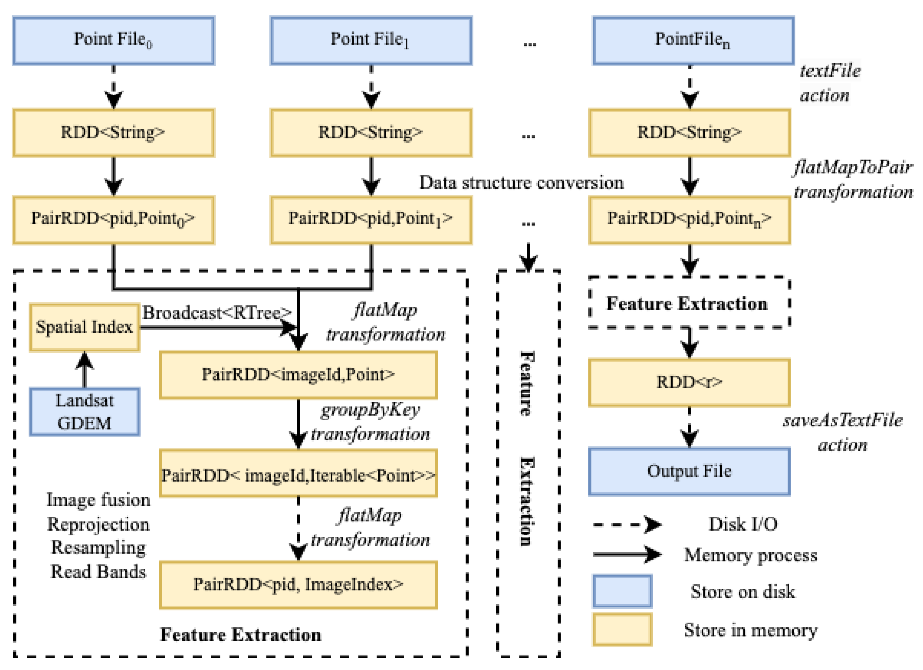
2.2.2. Stage 2: Parallel Matching of Samples and Images

Initial samples from existing land cover products only include longitude, latitude, and land cover labels, and they lack the features required for classifier input. The initial samples need to be matched with remote sensing images and auxiliary data in order to generate the final samples. There is a significant computational burden when matching samples and remote sensing images. The purpose of the process is to correspond the spatial positions of samples with the pixel positions of remote sensing images in order to read band information and perform calculations. The process of image matching includes the following: obtaining the image corresponding to the point through a spatial index; converting the longitude and latitude of the sample point to the plane coordinate system of the image; transforming it into the pixel row and column position through affine six-parameter transformation; and obtaining the average value in the window as the desired value. In the production process of GLC products, the number of remote sensing images reaches more than tens of thousands, and the number of spatial points in the training set can reach billions. The data volume of remote sensing images and auxiliary data can reach tens of terabytes. Traditional desktop software and unoptimized matching methods are unable to complete this process, so a more efficient matching method is needed to handle it. The HALF utilizes a parallel matching method for samples and images, as illustrated in Figure 4. The key to improving efficiency is to first establish an efficient correspondence relationship between samples and images through a spatial index, which is followed by distributing the reading tasks to each node. For each image, all matching points are read at once, thus avoiding the significant disk I/O pressure caused by frequent image reading. The method is illustrated as follows:

• Read all the center point data to be matched into memory; use the longitude and latitude of the point to form a unique identifier pid; read its spatial and attribute information to form a spatial point object; and compose a tuple <pid, Point>;
• Read the Landsat image metadata information; use the boundary coordinates to construct a spatial index STRtree; and use the broadcast variable in Spark to transmit it to each node. The broadcast variable will save a copy on each node, thus saving the network transmission cost for multiple calls;
• Distribute the computing tasks. To address the issue of data skew resulting from unequal allocation of images to different computing nodes during task distribution, a custom partitioning strategy was developed, and the groupByKey operator was used to allocate data evenly across all computing nodes as much as possible;
• For each image, parallel operations are performed using GDAL. Then, the image is subjected to image fusion, reprojection, and resampling, and the row and column numbers of the sample point’s longitude and latitude on the remote sensing image are calculated. If a sample is covered by clouds for most of the year or its quality is poor, it is discarded. The feature indicators are calculated for samples that meet the quality criteria, and both the data, along with their corresponding match results, are outputted.

2.2.3. Stage 3: Regional Adaptive Classification Model

The regional adaptive classification model was used to train the data in each region separately. Typically, the entire research area is divided into small areas, and the corresponding samples are used to train the model in each area adaptively. The classification results from all areas are merged to generate the final experimental outcomes. Although this approach may not be as straightforward in concept and implementation as global modeling, it overcomes the issue of overfitting due to small areas or underfitting due to large areas by sampling and training based on the unique characteristics of each region. Hankui [11] quantitatively compared the effectiveness of global modeling and adaptive modeling in the application of land cover in the United States, and their findings demonstrated that local modeling achieved greater classification accuracy than global modeling. In this study, the research area was segmented into a 10° × 10° grid.

The classifier provided by the HALF is a random forest model. Gómez et al. [48] compared various classification models, such as artificial neural networks, decision trees, support vector machines, random forests, and clustering in the mapping of land cover, and they found that the random forest algorithm has the advantages of insensitivity to noise, good anti-overfitting performance, and good robustness to data reduction. In addition, it is relatively simple to set the parameters, as only the number of trees and the number of features for decision tree branching need to be set. It is suitable for training data with different distribution features in multiple different partitions. Traditional accuracy metrics are derived from a confusion matrix such as overall accuracy (OA), producer accuracy (PA), user accuracy (UA), and kappa coefficient [49].

2.2.4. Stage 4: Parallel Mosaicking of Large-Area Classification Results

The size of a Landsat satellite image is 185 km × 185 km. Therefore, when producing large-area land cover products, multiple scenes need to be stitched together. The main purpose of image mosaicking is to convert the trained remote sensing images to the map and to output the final classification results. In this process, there were a huge number of images. If the images are stitched in serial order, the computational pressure will be enormous. Thus, a certain strategy needs to be adopted to solve the problem of low efficiency in the image merging process.

This process involves coordinate system transformation, image registration, and overlap area processing. Traditional image mosaicking methods first specify the coordinate system of one image as the reference and then register other images with it to determine the attribute values of corresponding coordinate points. If images are processed sequentially in this process, the computational efficiency is slow. The HALF utilized an image mosaicking method, and Figure 5 shows its schematic diagram. Traditional image processing operates on a per-image basis, and parallelism is not sufficient. In this study, the study area was divided into a grid of 10° × 10° cells. The spatial index was used to query the remote sensing images corresponding to each cell. Each cell was then subdivided into several smaller sub-images, with a specified resolution and edge length. After obtaining the spatial information of the sub-images, a blank image slice file corresponding to each sub-image was created through GDAL. The spatial relationship between each sub-image and the remote sensing image was established, and the row and column numbers on the remote sensing image were transformed to the corresponding row and column numbers on the sub-image through affine coordinate transformation. The specific values were written to the image slice file, and finally, all sub-images were merged into a complete classification result through the gdalbuildvrt and gdal_translate tools provided by GDAL. The spatial resolution of the customized product can also be used to complete the resampling work during the mosaicking process.

The parallel mosaicking method is demonstrated in Figure 6. The method first establishes the necessary parameters and determines the relationship between the sub-images and the remote sensing images. It then distributes tasks by using the sub-images as the parallel unit. When a sub-image corresponds to multiple remote sensing images, it first determines whether it is a no-data value. Otherwise, there may be a scenario where the invalid value will overwrite the valid value. Finally, it determines whether to output the latest results or all results based on the established rules. If the program is set to output multiple results, a blank view frame for multiple times is created to fill the corresponding sub-image with the corresponding results.

• Set the spatial extent, resolution, number of bands, and other parameters for different application scenarios. Then, create blank map sheets. For example, a latitude and longitude range of 10° × 10° corresponds to a grid of geographic extent of approximately 1100 km in length and width. If the sub-image resolution is set to 100 m, and each sub-image size is 256 × 256 pixels, then there are approximately 44 × 44 sub-images in this spatial range. The metadata information of the sub-images is stored in binary format, including spatial location and description, and files are created based on whether they already exist;
• Read the image information, and use the flatMap operator to match the spatial position of the sub-image with the metadata of the remote sensing image to establish a spatial correspondence. In this step, the key-value pairs of SubId and remote sensing images are obtained;
• Use the unique identification code pertaining to the SubId of the sub-image as the key to call the groupByKey operator to obtain the complete set of remote sensing images corresponding to each sub-image; the task is then distributed. Each task unit performs the sub-image filling task;
• In each task computing unit, perform coordinate transformation and row/column calculation for the image classification result, and fill in the corresponding pixel points for the sub-image. If no additional settings are made, the result from the latest remote sensing image corresponding to the sub-image is selected for writing.

2.3. HALF Workflow

The HALF provides workflow modules that encapsulate the key stages above through containers and organize each link using the workflow engine. The workflow model involves organizing remote sensing data, sample data, and processing functions into a structured and configurable set of steps. This approach enables practical problems to be resolved through automation or semi-automation. To encapsulate the model, the required basic environment image is searched and downloaded from the Docker Hub repository. Then, the necessary runtime environment is added, and the Docker commit command is used to create a new container image for storage. Relevant parameters of each model are recorded in XML description documents, while the basic model information is described in metadata files during registration. When adding a model, key details such as the model name, description, type, input parameters, output parameters, executable file path, dependent image, add time, user name, and test case are set. Metadata information of the operator is added to the database to complete the final model information storage and registration.

When organizing the workflow, use the Docker execution command as the Airflow workflow execution statement; access the database configured by Airflow; and monitor the running status of workflow nodes and instances. Airflow [50] is a lightweight workflow manager developed by AirBnB, Inc. Airflow provides a broad range of tools for managing the execution of workflows, such as pausing and resuming workflow execution, stopping and restarting individual workflow steps, and restarting workflows from a certain step. Airflow treats each workflow as a directed acyclic graph (DAG) of tasks with directional, non-cyclic dependencies. The DAG describes the relationships between tasks and defines their execution order. The Apache Foundation lists over 300 existing workflow languages and systems [51], and commonly used workflow systems in different fields have defined various organizational standards [52]. The international academic community has proposed the FAIR principles (Findable, Accessible, Interoperable, Reusable) for open and shared scientific data [53]. To this end, researchers have proposed the Common Workflow Language (CWL) [54], which entails a specification and standard for describing the creation of workflows that provides a universal standard for addressing the main issues in sharing workflows. The CWL describes the input and output of workflows in JSON or YAML format and has been applied in fields such as bioinformatics, hydrology, geospatial analysis, and physics. CWL-Airflow is one of the first workflow managers to support the CWL standard. It creates CWL-DAG instances based on workflow structure and executes them, followed by saving the results to an output folder.

The complete mapping process is presented in Figure 7. The research process consists of several stages encompassing sample generation, data matching, model training, image mosaicking, and data updating. The model description file specifies the parameters for each workflow node, and the input and output nodes for each workflow are designed accordingly.

In the HALF, users can establish models by describing the metadata information of workflow nodes in the description file and setting the input and output parameters of the nodes according to different application requirements. The HALF quickly builds workflows according to different application requirements to achieve customized management and monitoring. For the combined workflow model, the system provides a save function that records node parameter information and spatial location on the interface. After entering the workflow name and comments, the workflow model can be saved to the server for future use. It also allows users to monitor the running status of each step with multiple states such as success, running, waiting, and failure. Set the input and output of each node; the input can select the output of the previous node, and the input correction is carried out in this link to ensure that the output format of the previous node is filled in correctly.

2.4. Experimental Environment

The experimental environment consisted of a distributed cluster composed of three Dell Power Edge R720 servers, each with an Intel Xeon E5-2630 v2 2.60 GHz CPU and 30GB of RAM. The three machines shared a NAS storage of 20T. The experimental software and operating environment were Hadoop 2.7.6, Spark 2.3.4, Scala 2.11.8, JDK 1.8, Python 3.8.3 and GDAL 3.0.3(released by the Open Source Geospatial Foundation, Chicago, US).

The research creates container images for the models.

Table 2. Images environment configuration.

Images	Description	Base Images	Models
landuse-py	Used to run models written in Python	python:3.8.3	Sample Generation Classifier Training Image Classification Prediction
gdal-spark	Used to run models written in Java Spark	osgeo/gdal:ubuntu-full-3.6.3	Sample–Image Matching Image Mosaicking
pg12-citus-postgis	Used to storage metadata and spatial queries	postgres:12.14-alpine3.17	Building Spatial Index Spatial Querying
end-point	Used to launch the back-end project and provide network services	java:openjdk-8	Back-end Project

shows some of the images used for the runtime environment. The initial images were obtained from Docker Hub and further encapsulated to ensure that each model was portable and reusable.

3. Results

3.1. Model Performance Testing

We compared the deployment workload and execution time of the operators’ running tasks in containers and hosts. Deploying conventional applications on a physical machine may depend on multiple development and runtime environments, and the complexity of configuration depends on environment dependencies. For example, sample generation only requires a Python basic environment and GDAL to read images; the sample–image matching model is written in Java and also depends on Spark and GDAL; image training requires GDAL in the Python environment to fuse and resample images. The deployment of GDAL in the Python environment operating on the physical machine can be installed through conda, but the GDAL tool in the Java environment involves gcc compilation, which is extremely cumbersome. By pulling images provided on Docker Hub, the existing environment can be directly pulled and run, and the deployment workload is only one. Therefore, compared with the physical machine environment, the deployment efficiency can be effectively improved in the Docker container environment. Figure 8 shows the total time spent in production. The reason why the running time was longer in the Docker environment than in the physical machine environment is that the startup and destruction of Docker containers took some time, but the impact was very small in seconds. In addition, Docker containers themselves have the characteristic of light weight and will not occupy additional memory resources. In summary, deploying the model through Docker did not bring any losses in execution performance, but, compared to deploying the environment on a physical machine, it could reduce the configuration workload, thus making it convenient to migrate and reuse programs when deploying the production environment on new machines.

3.2. Automatically Generated Samples

Generating training samples based on existing land cover products makes it possible to obtain uniformly distributed samples at a large scale. The generated samples are visualized for several regions globally in Figure 9. The method guarantees complete automation of the entire classification process without any human intervention and ensures a large sample size and relatively uniform distribution in the sample space. Land cover classes such as water, bare area, or snow/ice tend to have higher discriminability during classification, thus resulting in denser sample points. On the other hand, classes such as cropland or grassland, which may have less distinct boundaries in different products, may exhibit more areas with “no samples” during classification. The classification system used for samples was inherited from previous products, thus eliminating the need for expert knowledge.

After matching, the generated sample set exhibited the characteristics illustrated in

Table 3. Descriptions of samples.

Feature	Data Source	Characteristic
Spatial Characteristics	Landsat	Longitude and Latitude
Temporal Characteristics		Image Acquisition Time
Spectral Characteristics		Band1, Band2…Band7
RS Index		NDVI, NDWI, EVI, NBR
Topographic Feature	DEM	DEM, Slope, Aspect
Land Cover Type	GLC	First-Level Type

, which included seven spectral features (bands), four remote sensing index features—Normalized Difference Vegetation Index (NDVI), Normalized Difference Water Index (NDWI), Enhanced Vegetation Index (EVI), Normalized Burn Ratio (NBR)—the latitude and longitude of the center point, the acquisition time of the image, and auxiliary indicators such as DEM, slope, and aspect.

3.3. Performance of Sample and Image Matching

In this section, we validated the method and conducted performance tests on different numbers of samples and remote sensing images.The experimental regions are shown in Figure 10, which include parts of Australia, Africa, and America. The longitude and latitude ranges for the Australian region were (110°E 40°S, 160°E 10°S), for the African region were (20°E 30°S, 50°E 10°N), and for the American region were (110°W 10°N, 50°W 40°N) and (80°W 50°S, 60°W 0°N). The method was able to complete the matching task within a short period of time when dealing with millions of samples and remote sensing images to be matched within a region. The execution time increased with the increase in samples and remote sensing images to be matched within a region.

To further validate the performance of the proposed method, the HALF matching method was set to Spark’s local computing mode and compared with the method based on GDAL under the same computing resources. The experimental task was to perform sample point–image matching on randomly selected 10,000 to 500,000 points from 131 images and to calculate the corresponding total time. Figure 11 shows that the proposed method not only had a significant advantage in running speed, but also was not affected by the sharp increase in point data volume in terms of running time stability. This is because the spatial relationship between points and images was first established using spatial indexing; as the number of points increased, the I/O overhead of the remote sensing images was relatively fixed.

In order to further investigate the performance of each step of the method,

Table 4. Time consumption analysis for each step of the matching method when data size is 100,000.

Stages	Time Cost(s)	GDAL	HALF
1	Build spatial index	0.7	0.7
2	Read data and create spatial relationships	4.2	2.6
3	Distribute tasks	/	4.9
4	Compute feature values	174.1	24.6
5	Total	179.2	32.8

provides a detailed breakdown of the time taken for each stage of the two methods at sample sizes of 100,000. The results show that the HALF matching method took significantly less time than the GDAL-based method in the stages of reading points and establishing spatial relationships, as well as reading image values and performing calculations, thereby demonstrating superior computational performance. At the same time, for different sample sizes, the time taken for the Spark-based matching method to distribute tasks to computing nodes increased, while the time taken to read image values and perform calculations remained relatively stable. This indicates that the custom partitioning strategy developed by the method effectively addressed the problem of uneven distribution of node images during task distribution, thus ensuring that the task completion time of each node was as close as possible, which maximized the use of computing resources and reduced computational time.

3.4. Performance of Large-Area Classification Result Mosaicking

Exploration of the performance of the proposed large-area image parallel mosaic method was conducted by selecting some 10° × 10° grids globally for experiments. The experimental regions are shown in Figure 12, which are the same as Figure 10. Furthermore, a thematic map was constructed based on the matching time of each grid area, where darker colors indicate longer algorithmic processing time.

A detailed analysis of the method performance in terms of processing time for the mosaic results of selected regions has been presented in

Table 5. Data volume and time consumption for partial regions.

Region	Spatial Extent	Number of Images	Number of Samples	Mosaic Time (s)	Match Time (s)
Region 1	(50°S–40°S, 70°W–60°W)	43	9,276,097	361	166.12
Region 2	(40°S–30°S, 70°W–60°W)	64	7,557,768	481	204.07
Region 3	(40°S–30°S, 140°E–150°E)	59	6,770,182	468	31.20
Region 4	(30°S–20°S, 20°E–30°E)	64	3,663,073	413	99.72
Region 5	(30°S–20°S, 140°E–150°E)	64	5,716,990	408	233.32
Region 6	(30°S–20°S, 130°E–140°E)	63	6,657,017	417	109.19
Region 7	(20°S–10°S, 110°E–120°E)	7	6,698,112	16	175.16
Region 8	(20°S–10°S, 20°E–30°E)	63	1,675,984	401	182.95
Region 9	(20°S–10°S, 30°E–40°E)	55	4,159,308	324	80.81
Region 10	(−10°S–0°N, 40°E–50°E)	13	11,522,471	72	169.84
Region 11	(30°N–40°N, 80°W–70°W)	31	16,008,303	222	143.02
Region 12	(0°N–10°N, 30°E–40°E)	62	1,022,583	359	119.86
Region 13	(10°N–20°N, 80°W–70°W)	35	9,698,301	250	134.51
Region 14	(20°N–30°N, 90°W–80°W)	39	12,549,213	253	146.13
Region 15	(20°N–30°N, 80°W–70°W)	34	11,688,087	224	153.62
Region 16	(30°N–40°N, 90°W–80°W)	63	12,793,479	439	259.34

. It was calculated that the average processing time for one image was around 6.5 s. For regions with around 60 images, such as regions 4 and 5, the calculation could be completed in around 400 s, while, for regions with around 30 images, such as region 11, it took over 200 s. As shown in the experimental results, with the increase in the number of images, the processing time of the mosaic method also gradually increased. Region 7 required only a little over 2 s to process one image on average, because only some parts of the region were land, and the sub-images not covered by any input images were not involved in the calculation. Among the selected regions, region 2 had the longest processing time, which was around 17% longer than that of region 4 and 5 with the same number of images. This is because Landsat images have deformation problems in different latitude regions, with larger image sizes in higher latitude regions, leading to longer processing time in high latitude regions. Further experiments were conducted to investigate the performance of the method under different regions and data volumes.

The study selected five regions with different latitudes that were all located on land. Figure 13 shows the changes in method runtime as the number of remote sensing images increased. To facilitate comparison, all these regions were located entirely on land. It was found that, regardless of the region, the method’s processing time showed a linear trend as the number of images increased. This is because, during the calculation, a correspondence was established between the sub-images and the remote sensing images, and the calculation tasks were distributed based on the sub-images. For each calculation task, the remote sensing images were traversed and calculated. Therefore, as the number of images increased, the method’s processing time increased almost linearly. In addition, the higher the latitude of the region, the more time it took to process the same number of images, because Landsat images at higher latitudes undergo distortion due to different projections, thereby resulting in larger image sizes and longer read times.

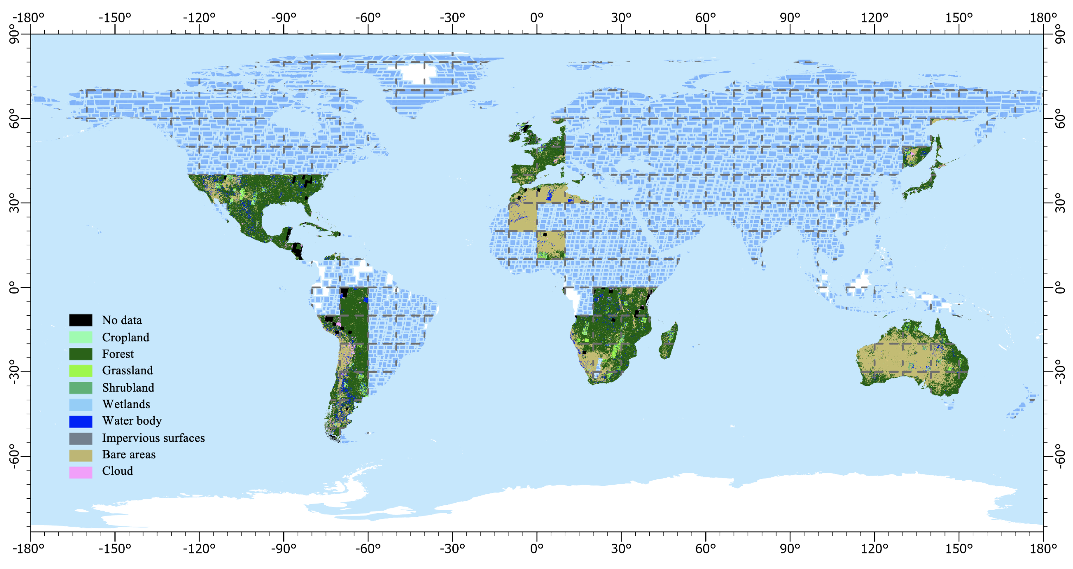
3.5. Result of Mapping

Figure 14 shows some regions around the world to present the classification results of the images. The results of the high-performance mosaicking method proposed were demonstrated by stitching together the classification results from regions such as Australia, Africa, and the Americas. The approach proposed in this study was effective for land mapping and could provide technical support to automate global land mapping.

Updating the classification results at the regional level could be performed on new incoming remote sensing images based on the results of the large-area mosaic method. As shown in Figure 15, there were missing data in some regions in the initial mapping result for the Korean Peninsula region. By querying the corresponding image row and column numbers based on spatial location information, new images could be inputted to fill in the missing areas. Figure 16 shows the process of updating existing products in the Japan region. In some areas, the product was affected by clouds, but higher-quality images could be used as input to update the obscured areas.

4. Discussion

The HALF framework presented in this study offers an automated and high-performance solution for large-area land cover mapping. By encapsulating each process’s models using container technology, the HALF addresses the issue of model heterogeneity between different processes, thus resulting in a significant reduction of deployment workload without sacrificing operational performance. The HALF integrated various stages in land cover mapping by using the CWL-Airflow workflow to organize and arrange the models, thus increasing the automation and flexibility. While the proposed method was experimentally verified for large-area and efficient mapping, there was a need for service publishing and sharing functions for workflows. Collaborative efforts between experts from various fields and countries are crucial for effective GLC mapping. The real-time sharing of models, processes, and data can have significant implications for land cover mapping.

The HALF provides a method of extracting a large number of samples from multiple sources of prior products. This method facilitates the generation of a large number of spatially distributed and evenly balanced samples, thereby significantly reducing the human and material resources that are utilized in the sample selection process. However, the accuracy of the samples generated by this method is affected by the prior products. In this study, many samples were generated by overlaying classification products automatically, and the first-level classes in the FROM_GLC and GLC_FCS products were extracted. The classification system chosen was relatively coarse, and the samples produced by this method were constrained by the accuracy of the prior products, thereby affecting the training of the classification model. In future research, the quality of the produced samples can be more rigorously controlled by adopting a more refined classification system. In addition, techniques such as change detection methods and transfer learning can be utilized to create a substantial number of uniformly distributed and high-precision samples.

The HALF optimized and accelerated sample feature matching and classification result mosaicking using high-performance computing technology. The specific effects of the method and its performance under different data volumes were discussed and explained in Section 3.4 and Section 3.5. The experimental results show that the matching method proposed in this study could quickly establish spatial relationships between points and images, and it could read image attributed to data in parallel, thereby effectively improving the computational efficiency of sample–image matching and feature extraction. Its efficiency was more than 10 times faster than conventional matching methods, and it performed well and stably under different data volume scenarios, thus making it applicable to other remote sensing applications that require large-area vector and raster data matching. The parallel mosaicking method for classification results used image slices as basic units, thereby achieving real-time mapping of large-area remote sensing image classification results to produce products and improving mapping efficiency. The total time required for resampling and mosaic of a single Landsat image in a 10° × 10° grid was about 6.5 s on average, thereby solving the problem of low computational efficiency when synthesizing multiple images. However, there may be practical difficulties in expanding the study area to the entire world, and the computational burden will increase exponentially with increasing research scope and resolution. Therefore, data fusion with other spatio-temporal resolution remote sensing data can be utilized to generate more real-time products if a higher update frequency is desired.

5. Conclusions

The process for producing large-area land cover products is complex, and as the demand for higher-resolution satellite remote sensing data and more frequent product updates increases, there is a growing need for automated tools and high-performance computing methods. The HALF aims to improve the operational efficiency of each link in the traditional process of land cover mapping in big data by utilizing high-performance computing technology. The HALF presents a method for large-area land cover mapping, which can serve as a valuable inspiration for researchers working on the development of remote sensing data processing or mapping tools. This is particularly beneficial for those who have limited access to paid computing power or require customization beyond existing platforms. To address the heterogeneity of operating systems, running environments, and programming languages between different links, container technology is used to encapsulate models such as sample generation, sample–image matching, model training and prediction, and classification result mosaicking, thereby supporting model reuse and data sharing, which greatly reduces the workload of deployment. Additionally, a general workflow language was introduced to model the land cover mapping process, organize data and models for each link, and decouple the production model from the overall process, thereby enhancing the automation and flexibility of the mapping process. In the future, we will further explore how to obtain higher-quality samples from multiple land cover products, encapsulate them into online data services with network technology, and integrate them into an integrated production portal to better support researchers in the field. By continuously improving the HALF, we can enhance the efficiency of large-area land cover mapping and better support global resource monitoring and sustainable development efforts.

References

1. Sterling, S.M.; Ducharne, A.; Polcher, J. The impact of global land-cover change on the terrestrial water cycle. Nat. Clim. Chang. 2013, 3, 385–390. [Google Scholar] [CrossRef]
2. Feddema, J.J.; Oleson, K.W.; Bonan, G.B.; Mearns, L.O.; Buja, L.E.; Meehl, G.A.; Washington, W.M. The Importance of Land-Cover Change in Simulating Future Climates. Science 2005, 310, 1674–1678. [Google Scholar] [CrossRef] [Green Version]
3. Ban, Y.; Gong, P.; Giri, C. Global land cover mapping using Earth observation satellite data: Recent progresses and challenges. ISPRS J. Photogramm. Remote Sens. 2015, 103, 1–6. [Google Scholar] [CrossRef] [Green Version]
4. Brown, C.F.; Brumby, S.P.; Guzder-Williams, B.; Birch, T.; Hyde, S.B.; Mazzariello, J.; Czerwinski, W.; Pasquarella, V.J.; Haertel, R.; Ilyushchenko, S.; et al. Dynamic World, Near real-time global 10 m land use land cover mapping. Sci. Data 2022, 9, 251. [Google Scholar] [CrossRef]
5. Yu, L.; Du, Z.; Dong, R.; Zheng, J.; Tu, Y.; Chen, X.; Hao, P.; Zhong, B.; Peng, D.; Zhao, J.; et al. FROM-GLC Plus: Toward near real-time and multi-resolution land cover mapping. Giscience Remote Sens. 2022, 59, 1026–1047. [Google Scholar] [CrossRef]
6. Sulla-Menashe, D.; Gray, J.M.; Abercrombie, S.P.; Friedl, M.A. Hierarchical mapping of annual global land cover 2001 to present: The MODIS Collection 6 Land Cover product. Remote Sens. Environ. 2019, 222, 183–194. [Google Scholar] [CrossRef]
7. Buchhorn, M.; Lesiv, M.; Tsendbazar, N.E.; Herold, M.; Bertels, L.; Smets, B. Copernicus Global Land Cover Layers—Collection 2. Remote Sens. 2020, 12, 1044. [Google Scholar] [CrossRef] [Green Version]
8. Chen, J.; Chen, J.; Liao, A.; Cao, X.; Chen, L.; Chen, X.; He, C.; Han, G.; Peng, S.; Lu, M.; et al. Global land cover mapping at 30m resolution: A POK-based operational approach. ISPRS J. Photogramm. Remote Sens. 2015, 103, 7–27. [Google Scholar] [CrossRef] [Green Version]
9. ESA WorldCover 10 m 2020 v100. Available online: https://zenodo.org/record/7254221 (accessed on 7 June 2023).
10. Li, X.; Gong, P. An “exclusion-inclusion” framework for extracting human settlements in rapidly developing regions of China from Landsat images. Remote Sens. Environ. 2016, 186, 286–296. [Google Scholar] [CrossRef]
11. Zhang, H.K.; Roy, D.P. Using the 500m MODIS land cover product to derive a consistent continental scale 30m Landsat land cover classification. Remote Sens. Environ. 2017, 197, 15–34. [Google Scholar] [CrossRef]
12. Radoux, J.; Lamarche, C.; Bogaert, E.V.; Bontemps, S.; Brockmann, C.; Defourny, P. Automated Training Sample Extraction for Global Land Cover Mapping. Remote Sens. 2014, 6, 3965–3987. [Google Scholar] [CrossRef] [Green Version]
13. Yu, L.; Wang, J.; Li, X.; Li, C.; Zhao, Y.; Gong, P. A multi-resolution global land cover dataset through multisource data aggregation. Sci. China Earth Sci. 2014, 57, 2317–2329. [Google Scholar] [CrossRef]
14. Wessels, K.J.; Van den Bergh, F.; Roy, D.P.; Salmon, B.P.; Steenkamp, K.C.; MacAlister, B.; Swanepoel, D.; Jewitt, D. Rapid Land Cover Map Updates Using Change Detection and Robust Random Forest Classifiers. Remote Sens. 2016, 8, 888. [Google Scholar] [CrossRef] [Green Version]
15. Zhang, X.; Liu, L.; Chen, X.; Xie, S.; Gao, Y. Fine Land-Cover Mapping in China Using Landsat Datacube and an Operational SPECLib-Based Approach. Remote Sens. 2019, 11, 1056. [Google Scholar] [CrossRef] [Green Version]
16. Zhang, X.; Liu, L.; Chen, X.; Gao, Y.; Xie, S.; Mi, J. GLC_FCS30: Global land-cover product with fine classification system at 30m using time-series Landsat imagery. Earth Syst. Sci. Data 2021, 13, 2753–2776. [Google Scholar] [CrossRef]
17. Venter, Z.S.; Barton, D.N.; Chakraborty, T.; Simensen, T.; Singh, G. Global 10 m Land Use Land Cover Datasets: A Comparison of Dynamic World, World Cover and Esri Land Cover. Remote Sens. 2022, 14, 4101. [Google Scholar] [CrossRef]
18. Shirani, K.; Solhi, S.; Pasandi, M. Automatic Landform Recognition, Extraction, and Classification using Kernel Pattern Modeling. J. Geovis. Spat. Anal. 2023, 7, 2. [Google Scholar] [CrossRef]
19. Gong, P.; Yu, L.; Li, C.; Wang, J.; Liang, L.; Li, X.; Ji, L.; Bai, Y.; Cheng, Y.; Zhu, Z. A new research paradigm for global land cover mapping. Ann. GIS 2016, 22, 87–102. [Google Scholar] [CrossRef] [Green Version]
20. Camargo, A.; Schultz, R.R.; Wang, Y.; Fevig, R.A.; He, Q. GPU-CPU implementation for super-resolution mosaicking of Unmanned Aircraft System (UAS) surveillance video. In Proceedings of the 2010 IEEE Southwest Symposium on Image Analysis & Interpretation (SSIAI), Chicago, IL, USA, 23–25 May 2010; pp. 25–28. [Google Scholar] [CrossRef]
21. Ma, Y.; Song, J.; Zhang, Z. In-Memory Distributed Mosaicking for Large-Scale Remote Sensing Applications with Geo-Gridded Data Staging on Alluxio. Remote Sens. 2022, 14, 5987. [Google Scholar] [CrossRef]
22. Zhang, J.; Ke, T.; Sun, M. Parallel processing of mass aerial digital images base on cluster computer—The application of parallel computing in aerial digital photogrammetry. Comput. Eng. Appl. 2008, 44, 12–15. [Google Scholar] [CrossRef]
23. Chen, C.; Tan, Y.; Li, H.; Gu, H. A Fast and Automatic Parallel Algorithm of Remote Sensing Image Mosaic. Microelectron. Comput. 2011, 28, 59–62. [Google Scholar]
24. Ma, Y.; Wang, L.; Zomaya, A.Y.; Chen, D.; Ranjan, R. Task-Tree Based Large-Scale Mosaicking for Massive Remote Sensed Imageries with Dynamic DAG Scheduling. IEEE Trans. Parallel Distrib. Syst. 2014, 25, 2126–2137. [Google Scholar] [CrossRef]
25. Jing, W.; Huo, S.; Miao, Q.; Chen, X. A Model of Parallel Mosaicking for Massive Remote Sensing Images Based on Spark. IEEE Access 2017, 5, 18229–18237. [Google Scholar] [CrossRef]
26. Rabenseifner, R.; Hager, G.; Jost, G. Hybrid MPI/OpenMP Parallel Programming on Clusters of Multi-Core SMP Nodes. In Proceedings of the 2009 17th Euromicro International Conference on Parallel, Distributed and Network-based Processing, Washington, DC, USA, 18–20 February 2009; pp. 427–436. [Google Scholar] [CrossRef]
27. Apache Hadoop. Available online: https://hadoop.apache.org (accessed on 20 April 2023).
28. Zaharia, M.; Chowdhury, M.; Franklin, M.J.; Shenker, S.; Stoica, I. Spark: Cluster computing with working sets. HotCloud 2010, 10, 95. [Google Scholar]
29. Garland, M.; Le Grand, S.; Nickolls, J.; Anderson, J.; Hardwick, J.; Morton, S.; Phillips, E.; Zhang, Y.; Volkov, V. Parallel Computing Experiences with CUDA. IEEE Micro 2008, 28, 13–27. [Google Scholar] [CrossRef]
30. Eldawy, A.; Mokbel, M. SpatialHadoop: A MapReduce framework for spatial data. In Proceedings of the 2015 IEEE 31st International Conference on Data Engineering, ICDE 2015. IEEE Computer Society, Proceedings—International Conference on Data Engineering, Seoul, Korea, 13–16 April 2015; pp. 1352–1363. [Google Scholar] [CrossRef]
31. Aji, A.; Wang, F.; Vo, H.; Lee, R.; Liu, Q.; Zhang, X.; Saltz, J. Hadoop GIS: A High Performance Spatial Data Warehousing System over Mapreduce. Proc. VLDB Endow. 2013, 6, 1009–1020. [Google Scholar] [CrossRef]
32. Shaikh, S.A.; Mariam, K.; Kitagawa, H.; Kim, K. GeoFlink: A Framework for the Real-time Processing of Spatial Streams. arXiv 2004, arXiv:2004.03352. [Google Scholar]
33. Kopp, S.; Becker, P.; Doshi, A.; Wright, D.J.; Zhang, K.; Xu, H. Achieving the Full Vision of Earth Observation Data Cubes. Data 2019, 4, 94. [Google Scholar] [CrossRef] [Green Version]
34. Nüst, D.; Konkol, M.; Pebesma, E.; Kray, C.; Schutzeichel, M.; Przibytzin, H.; Lorenz, J. Opening the publication process with executable research compendia. D-Lib Mag. 2017, 23, 451. [Google Scholar] [CrossRef]
35. Wang, B.; Zhang, M.; Huang, Q.; Yue, P. A Container-Based Service Publishing Method for Heterogeneous Geo-processing Operators. J. Geomat. 2021, 46, 174–177. [Google Scholar] [CrossRef]
36. Huffman, J.; Forsberg, A.; Loomis, A.; Head, J.; Dickson, J.; Fassett, C. Integrating advanced visualization technology into the planetary Geoscience workflow. Planet. Space Sci. 2011, 59, 1273–1279. [Google Scholar] [CrossRef]
37. Yue, P.; Zhang, M.; Tan, Z. A geoprocessing workflow system for environmental monitoring and integrated modelling. Environ. Model. Softw. 2015, 69, 128–140. [Google Scholar] [CrossRef]
38. Chen, Y.; Lin, H.; Xiao, L.; Jing, Q.; You, L.; Ding, Y.; Hu, M.; Devlin, A.T. Versioned geoscientific workflow for the collaborative geo-simulation of human-nature interactions—A case study of global change and human activities. Int. J. Digit. Earth 2021, 14, 510–539. [Google Scholar] [CrossRef]
39. Gesch, D.; Oimoen, M.; Danielson, J.; Meyer, D. Validation of the aster global digital elevation model version 3 over the conterminous united states. Int. Arch. Photogramm. Remote Sens. Spat. Inf. Sci. 2016, XLI-B4, 143–148. [Google Scholar] [CrossRef] [Green Version]
40. Gong, P.; Wang, J.; Yu, L.; Zhao, Y.; Zhao, Y.; Liang, L.; Niu, Z.; Huang, X.; Fu, H.; Liu, S.; et al. Finer resolution observation and monitoring of global land cover: First mapping results with Landsat TM and ETM+ data. Int. J. Remote Sens. 2013, 34, 2607–2654. [Google Scholar] [CrossRef] [Green Version]
41. Foody, G.M.; Arora, M.K. An evaluation of some factors affecting the accuracy of classification by an artificial neural network. Int. J. Remote Sens. 1997, 18, 799–810. [Google Scholar] [CrossRef]
42. Du, P.; Lin, C.; Chen, Y.; Wang, X.; Zhang, W.; Guo, S. Training Sample Transfer Learning from Multi-temporal Remote Sensing Images for Dynamic and Intelligent Land Cover Classification. J. Tongji Univ. (Nat. Sci. Ed.) 2022, 50, 955–966. [Google Scholar] [CrossRef]
43. Huang, Y.; Liao, S. Automatic collection for land cover classification based on multisource datasets. J. Remote Sens. 2017, 21, 757–766. [Google Scholar] [CrossRef]
44. Liu, K.; Yang, X.; Zhang, T. Automatic Selection of Clasified Samples with the Help of Previous Land Cover Data. J. -Geo-Inf. Sci. 2012, 14, 507–513. [Google Scholar] [CrossRef]
45. Tianjun, W.; Jiancheng, L.; Liegang, X.; Haiping, Y.; Zhanfeng, S.; Xiaodong, H. An Automatic Sample Collection Method for Object-oriented Classification of Remotely Sensed Imageries Based on Transfer Learning. Acta Geod. Cartogr. Sin. 2014, 43, 908. [Google Scholar] [CrossRef]
46. Anderson, J.R. A Land Use and Land Cover Classification System for Use with Remote Sensor Data; US Government Printing Office: Washington, DC, USA, 1976; Volume 964.
47. Gregorio, A.D.; Jansen, L.J.M. Land Cover Classification System (LCCS): Classification Concepts and User Manual; FAO: Geneva, Switzerland, 2000; ISBN 92-5-104216-0. [Google Scholar]
48. Gómez, C.; White, J.C.; Wulder, M.A. Optical remotely sensed time series data for land cover classification: A review. ISPRS J. Photogramm. Remote. Sens. 2016, 116, 55–72. [Google Scholar] [CrossRef] [Green Version]
49. Chaaban, F.; Khattabi, J.E.; Darwishe, H. Accuracy Assessment of ESA WorldCover 2020 and ESRI 2020 Land Cover Maps for a Region in Syria. J. Geovisualization Spat. Anal. 2022, 6, 31. [Google Scholar] [CrossRef]
50. Apache Airflow. Available online: https://airflow.apache.org (accessed on 20 April 2023).
51. Amstutz, P.; Mikheev, M.; Crusoe, M.R.; Tijanić, N.; Lampa, S. Existing Workflow Systems. Available online: https://s.apache.org/existing-workflow-systems. (accessed on 18 April 2023).
52. Leipzig, J. A review of bioinformatic pipeline frameworks. Briefings Bioinform. 2017, 18, 530–536. [Google Scholar] [CrossRef] [PubMed] [Green Version]
53. Schultes, E.; Wittenburg, P. FAIR Principles and Digital Objects: Accelerating Convergence on a Data Infrastructure; Springer International Publishing: Berlin/Heidelberg, Germany, 2019; pp. 3–16. [Google Scholar]
54. Common Workflow Language. Available online: http://www.commonwl.org (accessed on 20 April 2023).
Figure 1. The quantity and distribution of of Landsat8 images of 2015 used in the study.
Remotesensing 15 03143 g001
Figure 2. Framework of HALF.
Remotesensing 15 03143 g002
Figure 3. Schematic diagram of homogeneous region extraction.
Remotesensing 15 03143 g003
Figure 4. Parallel matching method for samples and remote sensing images.
Remotesensing 15 03143 g004
Figure 5. Schematic diagram of the mosaicking method for classification results. The world is partitioned into a grid system with each grid spanning 10° × 10°, and each grid is further divided into second-level sub-images. The blue border indicates the extent of the Landsat image, and when there are classification results within the grid, the pixels of the second-level sub-images within the spatial extent of the classification result are updated, and the final mosaic product is generated.
Remotesensing 15 03143 g005
Figure 6. The parallel mosaicking method for classification results.
Remotesensing 15 03143 g006
Figure 7. Conceptual design of the workflow. Describes the cartographic phase of HALF, with yellow nodes representing external data, green nodes representing computation results, blue nodes representing models, and red nodes representing classification models.
Remotesensing 15 03143 g007
Figure 8. Performance comparison between physical machine and container. (a) shows the comparison of time consumption, with various models on the horizontal axis and their corresponding running time on the vertical axis. (b) shows the comparison of deployment amount, with various models on the horizontal axis and an abstract estimate of deployment workload on the vertical axis.
Remotesensing 15 03143 g008
Figure 9. Automatically generated samples. The title of each subfigure indicates the latitude and longitude of the lower-left corner of the region. The legend is shown on the right side of each figure, and the white color indicates that there are no samples in this area.
Remotesensing 15 03143 g009
Figure 10. Time consumption statistics of the matching method.
Remotesensing 15 03143 g010
Figure 11. Performance comparison of matching method. The orange line indicates the time consumption of the matching method of HALF, and the blue line indicates the time consumption of the matching method of GDAL.
Remotesensing 15 03143 g011
Figure 12. Time consumption of the mosaicking method.
Remotesensing 15 03143 g012
Figure 13. Performance analysis of mosaicking methods.
Remotesensing 15 03143 g013
Figure 14. Large-area mosaic classification results.
Remotesensing 15 03143 g014
Figure 15. Update of regional classification results of the Korean Peninsula.
Remotesensing 15 03143 g015
Figure 16. Update of regional classification results of Japan.
Remotesensing 15 03143 g016