Article

Multilayer Data and Artificial Intelligence for the Delineation of Homogeneous Management Zones in Maize Cultivation

by
Diego José Gallardo-Romero
1,
Orly Enrique Apolo-Apolo
2,
Jorge Martínez-Guanter
3 and
Manuel Pérez-Ruiz
2,*
1
Departamento de Ingeniería Aeroespacial y Mecánica de Fluidos “Área Agroforestal”, Universidad de Sevilla, 41004 Sevilla, Spain
2
Department of Environment, Faculty of Bioscience Engineering, Ghent University, Coupure Links 653, Blok B, 1st Floor, 9000 Gent, Belgium
3
Corteva Agriscience, 41309 La Rinconada, Spain
*
Author to whom correspondence should be addressed.
Remote Sens. 2023, 15(12), 3131; https://doi.org/10.3390/rs15123131
Submission received: 28 April 2023 / Revised: 13 June 2023 / Accepted: 14 June 2023 / Published: 15 June 2023
(This article belongs to the Special Issue Monitoring and Control for Precision and Smart Agriculture)

Abstract

:
Variable rate application (VRA) is a crucial tool in precision agriculture, utilizing platforms such as Google Earth Engine (GEE) to access vast satellite image datasets and employ machine learning (ML) techniques for data processing. This research investigates the feasibility of implementing supervised ML models (random forest (RF), the support vector machine (SVM), gradient boosting trees (GBT), classification and regression trees (CART)) and unsupervised k-means clustering in GEE to generate accurate management zones (MZs). By leveraging Sentinel-2 satellite imagery and yielding monitor data, these models calculate vegetation indices to monitor crop health and reveal hidden patterns. The achieved classification accuracy values (0.67 to 0.99) highlight the potential of GEE and ML models for creating precise MZs, enabling subsequent VRA implementation. This leads to enhanced farm profitability, improved natural resource efficiency, and reduced environmental impact.

1. Introduction

The primary production sector, especially agriculture, is pivotal in driving the global economy, mitigating rural depopulation, and fostering economic development. Therefore, European sustainability strategies emphasize the importance of digital environments and advanced technologies in the agricultural sector, particularly those aimed at reducing inputs through variable applications, ensuring production efficiency, optimizing processes, and enhancing overall sustainability [1].
Management zones (MZs) have emerged by applying specific management strategies using the right amount of input at the right time and place [2], being a promising solution to address significant challenges in agriculture, including minimizing inputs via variable application rates, optimizing production efficiency, streamlining processes, and bolstering overall sustainability [1]. By establishing these zones, farmers can customize their management strategies to cater to the unique requirements of each zone, factoring in the spatial variability present within their fields. As a result, this targeted approach promotes more efficient resource utilization, ultimately supporting farming operations’ long-term sustainability and profitability. However, the delimitation of MZs in crop plots remains challenging due to the multiple factors contributing to spatial and temporal variability in the field. Factors such as soil variability (texture, structure, and water content), terrain topography (slope, orientation, and altitude), climatic conditions, crop genetic variability, or biotic influences contribute to remarkable and temporal variability in the field [3,4]. Despite the considerable amount of literature supporting the effectiveness of these techniques [5,6,7], precision agriculture techniques can present challenges and limitations for farmers for reasons such as cultural perception, access to technology, a lack of technical knowledge on the part of farmers themselves, or the high costs of implementing this type of technology [8].
The modernization of the agricultural sector encompasses many cutting-edge technologies beyond installing sensors in the field. These technologies are transforming agriculture by improving the efficiency and precision of farming practices. Within this wide range of technologies, we can highlight the use of remote sensors such as satellites and aerial imagery, artificial intelligence (AI), and big data to analyze large amounts of data, identify patterns, and predict variables. Cloud computing services allow the storage and processing of large volumes of data, providing greater computing capacity. In addition, nanotechnology is applied to developing new and improved chemical products. Robotics is used to automate tasks. Blockchain is used to track and verify the food supply chain. The crucial role of drones equipped with cameras and sensors for crop data collection, or the Internet of Things (IoT), is to establish a wireless connection between agricultural devices and sensors [9,10,11,12,13,14,15]. These technologies aim to enhance agricultural efficiency and improve sustainability [16,17]. This is where precision agriculture (PA) comes into play [18], with vegetation indices [19] being a significant contribution to agriculture since the 1970s, as they have provided an efficient and accurate way to assess vegetation health and vigor at different spatial and temporal scales [20].
In recent decades, remote sensing [21] has experienced significant advancements in sensor quality [22,23], leading to increased image resolution and enhanced dataset availability. This progress can be attributed to various satellite sources such as Landsat 8, Sentinel 2, or RapidEye, proximity remote sensing using RGB, multispectral and hyperspectral cameras, and terrestrial laser scanners (LIDAR), among many other devices. In addition, the great relevance of unmanned aerial vehicles (UAV) and other aerial platforms such as airplanes or helicopters should be highlighted. Developing new sensors, AI, big data techniques, and cloud computing platforms [24] will propel this trend further. Cloud computing platforms, such as Google Colab, Amazon Web Services (AWS), and Google Earth Engine (GEE) [25], offer efficient means for storing, accessing, and analyzing datasets on powerful servers [26]. On the other hand, machine learning (ML), which is a branch of AI [27], has demonstrated its potential for revolutionizing the agriculture sector [28]. ML algorithms can be broadly categorized into two main types: supervised learning (SL) and unsupervised learning (UL). SL focuses on predicting dependent variable values from independent variables [29], while UL aims to discover information, structures, or patterns in the data [30]. However, many agricultural plots lack crop monitoring due to factors such as limited resources, connectivity issues, a shortage of experts, or a lack of time and knowledge on the part of the farmer. This often results in missing data necessary for precision agriculture, such as yield monitor data and soil and crop moisture data. ML can address the limitations of agricultural plots by employing knowledge transfer models. These models are trained in accessible areas and then applied to hard-to-reach areas, enabling the application of ML in areas with limited resources or data availability. Another way to implement ML models in this type of plot would be by accessing and analyzing historical data, which could be used as input for model training. In addition, there would be the possibility to select a representative set of nearby plots with similar characteristics to the plot(s) with access limitations, train the models with these data, and ensure that the results and models apply to the rest of the plots. Consequently, VRAs on seeding or fertilization could be performed.
The objective of this research is to implement ML models, such as random forest (RF), support vector machine (SVM), gradient tree boosting (GTB), and classification and regression trees (CART), in conjunction with satellite data and yield monitors to identify management zones in study plots. By training these models, we aim to estimate the yield of other plots for which yield data are unavailable and automatically identify their zones. In addition, ground truth data and field yield data-based maps will validate the generated zones.

2. Materials and Methods

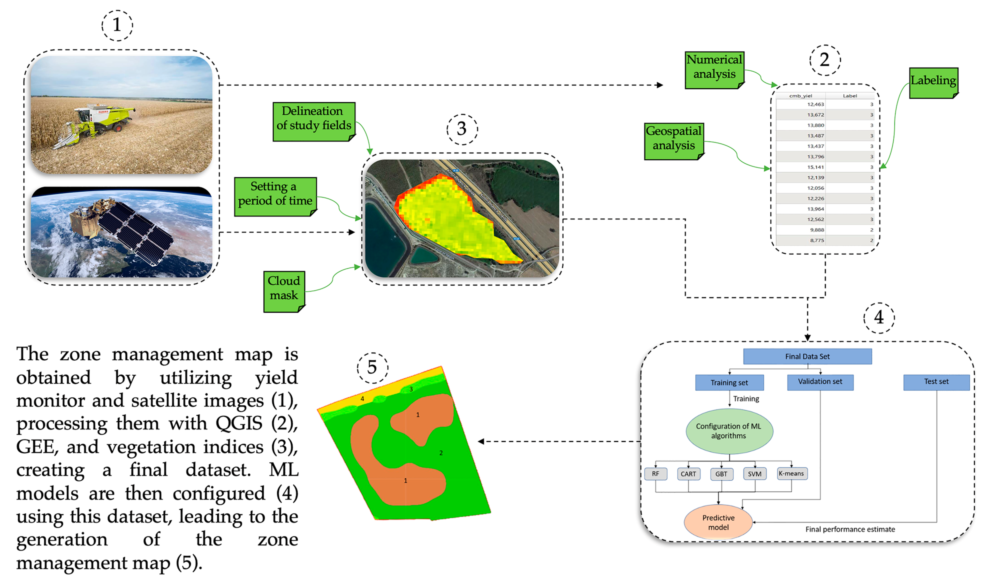
In this research, two data sources were employed to understand the spatio-temporal variability of agricultural plots and delineate management zones. Firstly, the GEE platform was utilized, providing access to a wide collection of high-resolution satellite images from different satellites. Then, using Sentinel-2 images, various vegetation indices were calculated, which provide relevant information about crops, such as the presence of stress, pests or diseases, or nutrient deficiencies, thereby evaluating the vegetative state of the crops. Additionally, yield data from multiple agricultural plots were collected using yield monitors installed in the harvesters. This allowed us to record detailed information regarding the production of the agricultural plots under study. The research flowchart, depicted in Figure 1, encompasses five distinct steps that were executed in this study.

2.1. Experimental Sites

The study was conducted in ten commercial fields cultivated with maize (Zea Mays L.) during the 2022 season. Fields were located in the Spanish provinces of Huesca, León, Salamanca and Zamora, as described in Table 1.
In addition to the above table showing the location of each of the study plots, Table 2 shows the agronomic data of these plots to facilitate the interpretation of the data obtained in the research.
Fields used as training and validation sets were planted between the 15th and 20th June 2022, and the harvesting dates were between the 4th and 28th December 2022, whereas the fields from Leon and Zamora used as a set of testing were planted on the 28th and 30th April 2022, respectively, and they were harvested on the 11th and 29th of November 2022. Yield data for each one of the fields were collected using a Claas Lexion 750 Montana combine harvester, equipped with a self-leveling system to compensate for uneven ground, an electro-mechanical guidance system, and a yield sensor to determine the quantity and quality of the harvested grain.

2.2. Analysis of Yield Data

The field-collected yield data from each plot, obtained using a yield sensor, necessitate two types of analysis. First, a numerical analysis must be performed to remove data that generate noise, such as null values, zeros, or other out-of-range values exhibiting significant variability compared to the mean. Second, a geospatial analysis is essential to examine the spatial behavior of the data and evaluate the influence of each data point on its neighboring values.
The raw performance data underwent two primary processes. The first process, numerical analysis, was conducted using an open-source geographic information system, QGIS v3.12 [31]. The second process involved a geospatial analysis carried out on the same QGIS platform. Then, using the Smart-Map plug-in [32], semivariograms, which provide information on the spatial variability of the data as a function of distances, and interpolations were generated using the ordinary Kriging method in conjunction with ML techniques [33], which use information from nearby sampling points to predict values at unsampled locations. These techniques were applied to create maps of management zones from the yield data, representing the reality on the ground. The maps obtained allow the spatial variations captured to be compared with the area maps generated by GEE from yield data and satellite images. After processing the data, it is essential to designate appropriate output labels for use in ML models used for zoning. In this case, yield values were categorized into three classes, as previous studies have shown no significant improvement in results using more than three classes. Therefore, it is generally recommended to delineate between three and five types [34,35,36,37,38]. Considering the yield data available after the elimination of outliers, it was decided to establish the following three classes. The first class consisted of yield values ranging from 1.00 to 7.99 tons per hectare (t/ha), the second class fell between 8.00 and 11.99 t/ha, and the third class was between 12.00 and 30.00 t/ha. This decision is based on the previous study of the data since it was carried out to obtain a dataset of classes with a certain degree of balance, containing several similar samples, to avoid biases in the ML models, improve generalization and robustness, and avoid overfitting problems [39]. In addition, agronomic reasons are taken into account so that the range of the third class (12.00–30.00 t/ha) is set taking into account that the average maximum yields at plot level in the northern areas of Spain, provided by the large seed companies with distribution in Spain, are placed in values of up to 22.4 t/ha in 2020, up to 20.6 t/ha in 2019, or up to 23.6 t/ha in 2018 [40]. Once the output labels have been designated, all maps are exported as a single shapefile, which can be imported into the GEE platform. Along with the vegetation index data obtained, this shapefile constituted the training-validation dataset for zoning. Following this approach, we can ensure that the ML models were trained on a high-quality dataset that accurately represents the different yield levels observed in the study area. This can lead to more accurate and reliable zoning results, which can ultimately help optimize agricultural management practices and improve crop yields.

2.3. Vegetation Indices

The GEE platform’s application program interface (API) [41] was used to calculate various vegetation indices and delineate MZs. This interface can be accessed through the web browser using the GEE code editor. The code editor provides an interactive interface where JavaScript code is developed and executed. Implementation in GEE involves following a series of steps, among which are data loading and manipulation, including the loading of geospatial data from the extensive library of datasets available in GEE and their manipulation through filtering, trimming, etc., operations using the JavaScript language; the analysis and processing of the data using a wide range of functions such as the generation of vegetation indices; the creation of predictive models using ML models; or the calculation of statistics and the visualization of the results in the form of interactive maps that allow the use of legends, colors, and selection of regions. A maximum cloudiness threshold of 20% was set for image selection and a cloud mask. The QA60 cloud mask refers to a quality band that is included in MSK_CLASSI and contains both opaque clouds (band 11) and cirrus clouds (band 10), with an indicator specifying the type of cloud (cirrus or opaque clouds). This mask contains information about the pixel quality in terms of cloud presence, cloud shadows, snow, water, or band saturation, among others. The mask determination method is composed of a series of steps such as atmospheric correction, the definition of a blue reflectance threshold for opaque clouds, the calculation of the snow index, and mask refinement [42].
The images collected from 5th July to 5th November 2022, for the training plots and from 5th June to 5th October 2022, for the test plots, covered approximately 36–38 days after sowing (DaS) and a BBCH 19 [43] growth stage, where the crop had approximately 20% ground cover, reducing soil reflectance. The start of the period was chosen to avoid problems with crop reflectance or obtaining low and unrepresentative values of the vegetative indices. The end date corresponded to a BBCH 87 growth stage, where the crop had approximately 80% ground cover and occurred before the onset of crop senescence. We highlight that the BBCH scale is a system for uniformly coding phonologically similar growth stages of all monocotyledonous and dicotyledonous plant species. The BBCH scale is a system for the uniform coding of phenologically similar growth stages in monocotyledonous and dicotyledonous plant species. This scale uses the base structures described by Zadoks in 1974 [44].
A total of 52 and 54 images were analyzed for the training and test plots, respectively. Ten published vegetation indices (Table 3) were calculated to assess the vegetative state of the crops. The objective was to select the index(es) that would provide the best classification accuracy, realism, and field implementability (Table 4).
At the GEE (Google Earth Engine) level, the most efficient approach to working with large datasets is to utilize time series that encompass the entire required period. However, handling such extensive datasets becomes challenging without applying reduction functions provided by GEE. These reduction functions offer three options: ee.Reducer.min(), ee.Reducer.median(), and ee.Reducer.max(). In this study, the reduction function that calculates the mean was implemented, as depicted in Figure 2.
r e s i z e d I m a g e = o r i g i n a l I m a g e . r e p r o j e c t ( c r s : o r i g i n a l I m a g e . p r o j e c t i o n ( ) s c a l e : n e w S c a l e )
where originalImage is the original image to be resized; reproject () is the GEE function used to change the image projection; crs: originalImage.projection specifies the output projection for the resized image. In the case under study, the same projection of the original image is used; scale defines the new scale for the resized image, where newScale is the desired scale value in meters.

2.4. Machine Learning Models

In addition to offering functions for calculating spatial and spectral operations, the GEE platform provides other mathematical functions and advanced ML algorithms, both supervised and unsupervised [55]. The dataset was partitioned into a 70–30% split for training and validation, resulting in 8670 data points for training and 3717 data points for validation. A series of steps were taken to combine the data from the different sources. Once the yield data, the satellite images corresponding to the defined period and the vegetation indices have been imported, the training and validation datasets are prepared. For this purpose, many feature collections based on the yield data are defined as zones to be used, in this case, three zones. In these zones, the filter.lt and filter.gte functions are used to split the data into 70–30%. The merge function is then used on both the training and validation data to merge the defined zones into a single variable. Next, the sampleRegions function is used, which takes as input the vegetation indices calculated for the image collection and the previously defined training variable containing the performance-based zone labels. Finally, the ML models are implemented, which take as their training dataset the training variable with the performance data and the calculated vegetation indices. The general equation to implement the indices would be as follows:
C l a s s i f i c a t i o n = e e . C l a s s i f i e r . M L m o d e l ( ) . t r a i n ( t r a i n i n g v a r i a b l e , c o l u m n z o n e s , v e g e t a t i o n i n d e x )
where training variable refers to the performance data file, “column zone” is the name of the column of the performance data file containing the classes that have been defined before loading the dataset into GEE, and vegetative index is the band originating from the calculation of the index to be used.
Four supervised ML algorithms, including classification and regression tree (CART), random forest (RF), gradient boosting trees (GBT), and support vector machine (SVM), were implemented. The CART algorithm is a statistical procedure that identifies mutually exclusive and exhaustive subgroups of a population based on common characteristics [56]. During the investigation, only the parameter minLeafPopulation = 1 was considered, so that the generated nodes contained at least one point. RF is a set of decision trees that reduces overfitting and improves prediction accuracy using different subsets of data and features [57,58]. In the case study, 100 trees were used to perform training and subsequent classification. GBT is another ensemble method that trains trees sequentially, fitting each new tree based on the residuals of the previous trees, resulting in a weighted combination of all previous models [59,60]. As in RF, 100 trees are used. The rest of the parameters employed use the default values defined in the function itself. SVM, on the other hand, finds the optimal hyperplane to separate the observations into classes based on the features [61]. In this case, the implementation of this algorithm is carried out with the default values of each of the parameters that compose it. The k-means clustering algorithm was also implemented to compare its performance with the supervised classification models based on yield values and vegetation indices. K-means is an unsupervised clustering method that groups data points into clusters based on feature similarity [62]. It starts with a set of random centroids and performs repetitive calculations to optimize the position of the centroids.

2.5. Evaluation Metrics and Delineation of Homogeneous Management Zones

ML models must be evaluated using specific metrics to test their robustness [63]. This research used two popular accuracy indicators, namely the overall accuracy (Equation (3)) and the Kappa coefficient (Equation (4)), to evaluate the supervised classification algorithms used in the GEE platform.
A c c u r a c y = T r u e   P o s i t i v e s T r u e   p o s i t i v e s   +   F a l s e   P o s i t i v e s
where true positives (TP) are the positive cases correctly classified as positive by the model, and false positives (FP) are the negative cases incorrectly classified as positive by the model.
K = P o P e 1 P e
where Po is the observed proportion of agreement between raters or evaluators. It is calculated by dividing the number of observed agreements by the total number of ratings performed, and Pe is the expected proportion of agreements due to chance. It is calculated by multiplying the marginal proportions of the ratings separately and summing up the results [64].
For the authors of [65] (pp. 111–115), overall accuracy is defined as the proportion of correct model predictions in the training dataset and is calculated by dividing the number of accurate predictions by the total number of predictions. However, overall accuracy may not always be the most useful measure since, if the classes are unbalanced, the accuracy values may be somewhat misleading. In these cases, the Kappa coefficient may be the right metric, as it measures the agreement between true labels and predictions, considering the distribution of classes [66]. However, for the clustering algorithm used, k-means, a visual interpretation of the results was performed, taking as a reference the performance maps generated through kriging in QGIS. The calculation of these metrics requires the prior calculation of the confusion matrix, which is a fundamental tool in the evaluation of classification models. It generates a table that shows the number of instances classified correctly and incorrectly by the model. TP indicates the instances that are positive and were classified correctly; true negative (TN) indicates the instances that are negative and were classified correctly; FP indicates the instances that are negative and were incorrectly classified as positive; and false negatives (FNs) indicate the positive instances that were incorrectly classified as negative [67].
Metrics that have been used to assess the accuracy of maps generated as ground truth using the Smart-Map plug-in are root mean square error (RMSE), defined as the difference between predicted and actual values in regression models, and the coefficient of determination (R2), which measures the variability of the data in the range 0–1, where 0 explains no variability and 1 explains all variability [68].
Finally, after the classification of the data using ML algorithms, an isolated pixel attenuation method was used, which applies a morphological reducer to each band of the image using an octagonal kernel of radius 6 m, allowing mapping criteria such as the minimum mappable area to be met, facilitating its use in agricultural machinery and its use in the field.

3. Results

3.1. Variability and Geospatial Mapping of Crop Plot Yields

The analysis of the inter-plot variability of the yield data revealed that the most suitable models were linear and spherical, with two cases showing exponential trends. Furthermore, the prediction accuracy metrics used to evaluate the fit of these models showed high accuracy, as evidenced by the R-squared values being very close to 1 and the RMSE values being close to 0. The lower the RMSE value, the higher the accuracy of the model (see Table 5). This indicates that the values fit well with the models used for interpolation, both for the training plots and the test plots.
The geospatial maps of the two plots, generated using the ordinary kriging function of the QGIS Smart-Map plug-in, revealed five distinct zones (see Figure 3). Based on this differentiation and the number of zones, management zone maps for both plots were created using the same plug-in, which showed the same pattern as the maps generated through interpolation (see Figure 4). In both plots, the low-yield zone was mainly attributed to areas near the plot’s edges, particularly in the headlands. In the plot in Cabreros del Río, León, low-yield zone 1 was situated towards the plot’s edges, especially in the headland area, while the highest-yield zone was located in the middle-lower area of the plot. As for the plot in Coreses, Zamora, zone 1 of lower yield was also situated at the plot’s edges, with a more pronounced effect in the headland and lower part of the plot. The high-yield zones were distributed, intermingled with zone 2 of medium yield throughout the plot.

3.2. Accuracy of Generated ML Models and Classification Maps

The generation of maps using ML models requires assessing the classification accuracy, for which the overall accuracy (Table 6) and the Kappa coefficient (Table 7) were used for each of the proposed indices.
The RF and CART models achieved the highest accuracy and Kappa coefficient values, exceeding 0.90. The RF model, which is an ensemble model that combines multiple decision trees trained on random data samples to improve accuracy and reduce overfitting, was more robust than other models were, leading to its higher accuracy. Similarly, the CART model’s capacity to divide data into smaller subsets based on crucial characteristics can improve the interpretation and classification of the data, particularly with categorical variables [69]. Hence, based on the high accuracy achieved by the CART model, it was selected for the classification of the two test plots in León (Figure 5) and Zamora (Figure 6).
Comparing the zone map generated by the Smart-Map plug-in based on yield data from the León plot (Figure 4) with the maps generated by the CART model for the same plot (Figure 5), it was observed that all indices exhibited similar patterns related to the yield map. In addition, all indices had differentiated values around the plot’s perimeter, with isolated high-value areas in the interior. This is because of the edge effect caused in agricultural plots. This effect is caused by different factors, such as the excessive passage of agricultural machinery during operations, competition with weeds, physical damage caused by the wind, and the presence of roads along the perimeter of the plot, which leads to sediment runoff from the roads into the plot. Notably, the SIPI index identified a distinct high-yield zone in the lower-middle area of the plot, which was also apparent in the yield map.
These results indicate that machine learning algorithms, such as CART and RF, can provide accurate predictions of crop yield based on remote sensing data. Hence, machine learning and geospatial analysis techniques provide a valuable tool set for agricultural researchers and practitioners seeking to enhance crop yield predictions and optimize management practices. By leveraging these methods, we can gain valuable insights into the spatial variability of crop yield, identify factors contributing to yield variation, and develop management strategies to improve overall productivity.
Factors contributing to variation in final crop yield that could be detected by vegetation indices include the presence of water or heat stress, nutritional deficiencies, or the presence of pests and diseases [70,71,72].
A similar comparison was made between the zone map generated by Smart-Map using the yield data from the Zamora plot (Figure 4) and the maps obtained using the CART model (Figure 6). The yield zone map showed the most significant variations in the perimeter zones of the plot, while zone three predominated in the interior zone, which was eclipsed by zone two values in the eastern and western parts. The maps generated by the CART model exhibited the same pattern in the perimeter zones of the plot as the yield zone map. Still, there were differences in the interior part, likely due to the non-significant difference in the values of each of the vegetative indices calculated.
Like SL models, the k-means algorithm aims to identify spatial patterns in test plots, providing valuable information about their distribution. Figure 7 presents the maps generated based on various vegetation indices for the León test plot. Although all maps exhibit some similarity to the yield zone map obtained for the 2022 season in this plot (Figure 4), the modified chlorophyll absorption ratio index (MCARI) map is the most similar, as it identifies a distinct area in the mid-lower part of the plot that corresponds to a differentiated area in the yield zone map. Additionally, the MCARI index exhibits a pattern close to that of the plot’s edges.
The maps generated using the k-means algorithm for the Zamora field (Figure 8) revealed an interesting peculiarity. Despite identifying the base pattern observed in the yield zone map (Figure 4), where the differentiation between the headland and border zones and the rest of the plot is apparent, several indices, such as ARVI, EVI, MSAVI2, NDRE, and SIPI, exhibited a two-zone classification when applied to the k-means model. This was likely due to the similarity in their values, which prevented the k-means model from establishing a three-zone classification.

3.3. Management Zone Maps for Variable Application

Maps generated using ML classification algorithms use isolated pixels, which are unsuitable for having management zones that can be easily integrated into agricultural machinery and reproduced in the field. Consequently, a morphological filter was applied to the maps of the two test plots (León and Zamora) generated, which converted the maps in (Figure 5 and Figure 6) into maps with management zones adaptable to the field without losing sight of the pattern identified by the classification of the ML models (Figure 9 and Figure 10).

4. Discussion

The findings presented in this research highlight the immense potential of integrating machine learning models with satellite data and yield monitors to effectively identify MZs in the cloud using GEE. Prior to this study, numerous researchers, such as Quebrajo et al. [1], had employed time-consuming and manual techniques for creating management zones, which are not ideal from a precision agriculture standpoint. However, with the utilization of ML models in conjunction with satellite data and yield monitors, the process can be significantly streamlined and optimized for PA applications.
The GEE platform is one of the most efficient geospatial data analysis and processing tools. The GEE platform is a very effective geospatial data analysis and processing tool, providing access to large volumes of satellite data, including Sentinel-2 data. Unlike studies such as [73,74], where field data are used to perform zonal management in maize cultivation, the GEE platform allows the obtention of accurate and up-to-date data on crop vegetative status remotely without the need to take field data [75]. This makes it possible to monitor plots that are difficult to access. An example of this would be agricultural plots located in mountainous or hard-to-reach areas due to the terrain’s topography. Plots are located in protected environments or natural reserves, where access restrictions are often imposed to protect biodiversity and ecosystems. It is also worth noting those plots of extensive crops with large surfaces, due to their size, can make it challenging to access all areas.
GEE’s cloud-based platform does not require internal storage, streamlining work and the elimination of expensive hardware and software. In addition, GEE enables the implementation of ML techniques and models. The segmentation and classification of satellite images using ML techniques, both supervised, such as RF or CART, and unsupervised, such as k-means, allow the identification of patterns in the data and the understanding of the spatial and temporal variability of the plot to perform agricultural practices in a targeted manner [76]. Applying these techniques allows for more sustainable agricultural management by generating maps of management zones that will enable much more accurate planning of agricultural work and identify areas that require fewer inputs, leading to a reduction in production costs and a possible improvement in the quality and yield of crops.
These results indicate that machine learning algorithms, such as CART and RF, can provide accurate predictions of crop yield based on remote sensing data. Furthermore, using geospatial analysis tools, such as Smart-Map, can help identify and delineate areas of high and low yield variability, which could help optimize management practices and improve overall crop yields. These findings have important implications for precision agriculture. They can help farmers make informed decisions on input applications, irrigation management, and crop rotations, leading to more efficient resource use and increased profitability.
In comparison to previous research such as [77,78], where MZs were established in corn by downloading satellite images and subsequently processing them, the utilization of GEE provides the advantage of automatically generating zone maps without the need to download the images or bands. This significantly streamlines the process and eliminates the additional steps involved in data acquisition. Furthermore, when compared to other studies such as [79,80], which reported Kappa coefficient values ranging from 0.32 to 0.79 and 0.63 to 0.73, respectively, the ML models employed in this research demonstrated significantly higher values. Particularly, the CART and RF models exhibited superior performance, with Kappa coefficient values ranging from 0.90 to 0.99. These findings highlight the enhanced accuracy and reliability achieved through the implementation of these machine learning models in conjunction with GEE, surpassing the results obtained in earlier studies.
Although there is room for improvement in the results, particularly with respect to the availability of a more comprehensive dataset that includes a larger number of fields, it can be summarized that this research showcases the potential of integrating advanced technologies such as GEE, remote sensing, and ML models with farm management practices. By combining these techniques, valuable and timely crop information can be obtained, resulting in enhanced decision making processes and optimized resource allocation through variable rate application. The study highlights the significance of leveraging these cutting-edge technologies to improve agricultural practices and achieve more efficient and precise agricultural outcomes.

5. Conclusions

The findings of this manuscript demonstrate the effectiveness of integrating both supervised (CART, GBT, RF, and SVM) and unsupervised (k-means) ML models with GEE and Sentinel-2 imagery for vegetative crop monitoring and the automated generation of agricultural management area maps based on vegetation indices. This innovative approach offers a valuable solution that has the potential to replace specific field data collection tasks that may be challenging to conduct due to economic constraints, agricultural limitations, or accessibility issues.
Looking ahead, the future holds the promise of free access to multispectral optical satellite images with lower resolutions than those of the current standards. This anticipated advancement opens doors for the further development and refinement of agricultural applications for MZs with even greater precision. By capitalizing on these improved data sources, future research can expand the scope and accuracy of ML models in precision agriculture, enabling more informed decision making processes for farmers.

Author Contributions

All authors contributed to the article and approved the submitted version. D.J.G.-R. wrote the first draft of the manuscript, took the field measurements, and analyzed the data; O.E.A.-A. took the field measurements and provided suggestions on the manuscript; J.M.-G. provided suggestions on the structure of the manuscript, participated in the discussions of the results and acquired funding; M.P.-R. conceived the experiments, supervised them, and acquired funding. All authors have read and agreed to the published version of the manuscript.

Funding

This research was funded by the Government of Andalusia, Regional Ministry of Economic Transformation, Industry, Knowledge and Universities, grant number PYC20 RE 082 USE.

Data Availability Statement

Not applicable.

Acknowledgments

The authors would like to express their gratitude to the “AGR-278; Smart Biosystems Lab” research group for their unwavering support throughout this study.

Conflicts of Interest

The authors declare that the research was conducted without any commercial or financial relationships that could be construed as potential conflicts of interest.

References

  1. Quebrajo, L.; Pérez-Ruiz, M.; Rodriguez-Lizana, A.; Agüera, J. An Approach to Precise Nitrogen Management Using Hand-Held Crop Sensor Measurements and Winter Wheat Yield Mapping in a Mediterranean Environment. Sensors 2015, 15, 5504–5517. [Google Scholar] [CrossRef] [Green Version]
  2. Zhang, N.; Wang, M.; Wang, N. Precision Agriculture—A Worldwide Overview. Comput. Electron. Agric. 2002, 36, 113–132. [Google Scholar] [CrossRef]
  3. Fanelli, R.M. The Spatial and Temporal Variability of the Effects of Agricultural Practices on the Environment. Environments 2020, 7, 33. [Google Scholar] [CrossRef] [Green Version]
  4. Vélez, S.; Rançon, F.; Barajas, E.; Brunel, G.; Rubio, J.A.; Tisseyre, B. Potential of Functional Analysis Applied to Sentinel-2 Time-Series to Assess Relevant Agronomic Parameters at the within-Field Level in Viticulture. Comput. Electron. Agric. 2022, 194, 106726. [Google Scholar] [CrossRef]
  5. Cheng, E.; Zhang, B.; Peng, D.; Zhong, L.; Yu, L.; Liu, Y.; Xiao, C.; Li, C.; Li, X.; Chen, Y.; et al. Wheat Yield Estimation Using Remote Sensing Data Based on Machine Learning Approaches. Front. Plant Sci. 2022, 13, 1090970. [Google Scholar] [CrossRef]
  6. Mallarino, A.P.; Wittry, D.J. Efficacy of Grid and Zone Soil Sampling Approaches for Site-Specific Assessment of Phosphorus, Potassium, PH, and Organic Matter. Precis. Agric. 2004, 5, 131–144. [Google Scholar] [CrossRef]
  7. Shafi, U.; Mumtaz, R.; García-Nieto, J.; Hassan, S.A.; Zaidi, S.A.R.; Iqbal, N. Precision Agriculture Techniques and Practices: From Considerations to Applications. Sensors 2019, 19, 3796. [Google Scholar] [CrossRef] [Green Version]
  8. Zarco-Tejada, P.J.; Hubbard, N.; Loudjani, P. Precision Agriculture: An Opportunity for EU-Farmers-Potential Support with the CAP 2014–2020; European Parliament: Brussels, Belgium, 2014. [Google Scholar]
  9. Atzori, L.; Iera, A.; Morabito, G. Understanding the Internet of Things: Definition, Potentials, and Societal Role of a Fast Evolving Paradigm. Ad Hoc Netw. 2017, 56, 122–140. [Google Scholar] [CrossRef]
  10. Zhang, C.; Kovacs, J.M. The Application of Small Unmanned Aerial Systems for Precision Agriculture: A Review. Precis. Agric. 2012, 13, 693–712. [Google Scholar] [CrossRef]
  11. Lira Saldivar, R.H.; Méndez Argüello, B.; De los Santos Villareal, G.; Vera Reyes, I. Potencial de La Nanotecnología en la Agricultura. Acta Univ. 2018, 28, 9–24. [Google Scholar] [CrossRef]
  12. Mirabelli, G.; Solina, V. Blockchain and Agricultural Supply Chains Traceability: Research Trends and Future Challenges. Procedia Manuf. 2020, 42, 414–421. [Google Scholar] [CrossRef]
  13. Ahirwar, S.; Swarnkar, R.; Bhukya, S.; Namwade, G. Application of Drone in Agriculture. Int. J. Curr. Microbiol. Appl. Sci. 2019, 8, 2500–2505. [Google Scholar] [CrossRef]
  14. Shao, G.; Han, W.; Zhang, H.; Zhang, L.; Wang, Y.; Zhang, Y. Prediction of Maize Crop Coefficient from UAV Multisensor Remote Sensing Using Machine Learning Methods. Agric. Water Manag. 2023, 276, 108064. [Google Scholar] [CrossRef]
  15. Boursianis, A.D.; Papadopoulou, M.S.; Diamantoulakis, P.; Liopa-Tsakalidi, A.; Barouchas, P.; Salahas, G.; Karagiannidis, G.; Wan, S.; Goudos, S.K. Internet of Things (IoT) and Agricultural Unmanned Aerial Vehicles (UAVs) in Smart Farming: A Comprehensive Review. Internet Things 2022, 18, 100187. [Google Scholar] [CrossRef]
  16. Nasser Alsammak, H.; Saeed Mohammed, D. Internet of Things (IoT) Work and Communication Technologies in Smart Farm Irrigation Management: A Survey. NTU J. Eng. Technol. 2022, 1, 49–65. [Google Scholar]
  17. Ramón Fernández, F. Inteligencia Artificial y Agricultura: Nuevos retos en el sector agrario. Campo Jurídico 2020, 8, 123–139. [Google Scholar] [CrossRef]
  18. Castellanos, R.M.; Morales-Pérez, M. Análisis Crítico Sobre La Conceptualización de La Agricultura de Precisión. Cienc. PC 2016, 2, 23–33. [Google Scholar]
  19. Gitelson, A.A.; Kaufman, Y.J.; Stark, R.; Rundquist, D. Novel Algorithms for Remote Estimation of Vegetation Fraction. Remote Sens. Environ. 2002, 80, 76–87. [Google Scholar] [CrossRef] [Green Version]
  20. Bannari, A.; Morin, D.; Bonn, F.; Huete, A.R. A Review of Vegetation Indices. Remote Sens. Rev. 1995, 13, 95–120. [Google Scholar] [CrossRef]
  21. Andreu, A.; Carpintero, E.; González-Dugo, M.P. Teledetección Para Agricultura; Instituto de Investigación y Formación Agraria y Pesquera (IFAPA): Sevilla, Spain, 2021; pp. 1–41. [Google Scholar]
  22. Khanal, S.; Kushal, K.C.; Fulton, J.P.; Shearer, S.; Ozkan, E. Remote Sensing in Agriculture—Accomplishments, Limitations, and Opportunities. Remote Sens. 2020, 12, 3783. [Google Scholar] [CrossRef]
  23. Yuste Martín, Y.; Vargas-Velasco, N.; Moya-Hernández, J. Teledetección Ambiental de Alta Resolución Mediante Aplicación de Vehículos Aéreos No Tripulados. Soc. Esp. Defic. For. 2013, 1–22. Available online: https://www.congresoforestal.es/actas/doc/6cfe/6cfe01-451.pdf (accessed on 27 April 2023).
  24. Nakar, D. Sentinel-2: Multispectral Instrument (MSI) Design and System Performance. 2019. Available online: https://www.researchgate.net/publication/334432047_Sentinel-2_Multispectral_Instrument_MSI_design_and_system_performance (accessed on 27 April 2023).
  25. Gorelick, N.; Hancher, M.; Dixon, M.; Ilyushchenko, S.; Thau, D.; Moore, R. Google Earth Engine: Planetary-Scale Geospatial Analysis for Everyone. Remote Sens. Environ. 2017, 202, 18–27. [Google Scholar] [CrossRef]
  26. Amani, M.; Ghorbanian, A.; Ahmadi, S.A.; Kakooei, M.; Moghimi, A.; Mirmazloumi, S.M.; Moghaddam, S.H.A.; Mahdavi, S.; Ghahremanloo, M.; Parsian, S.; et al. Google Earth Engine Cloud Computing Platform for Remote Sensing Big Data Applications: A Comprehensive Review. IEEE J. Sel. Top. Appl. Earth Obs. Remote Sens. 2020, 13, 5326–5350. [Google Scholar] [CrossRef]
  27. Domingos, P. A Few Useful Things to Know about Machine Learning. Commun. ACM 2012, 55, 78–87. [Google Scholar] [CrossRef] [Green Version]
  28. El Naqa, I.; Li, R.; Murphy, M. Machine Learning in Radiation Oncology; Springer: Berlin/Heidelberg, Germany, 2019. [Google Scholar]
  29. González, F.A. Machine learning models in rheumatology. Rev. Colomb. Reumatol. 2015, 22, 77–78. [Google Scholar]
  30. Fuentes Hurtado, F.J. Aprendizaje No Supervisado; Universidad Internacional de Valencia, España: València, Spain, 2019; pp. 9–12. [Google Scholar]
  31. Moyroud, N.; Portet, F. Introduction to QGIS. QGIS Generic Tools 2018, 1, 1–17. [Google Scholar]
  32. Pereira, G.W.; Valente, D.S.M.; Queiroz, D.M.d.; Coelho, A.L.d.F.; Costa, M.M.; Grift, T. Smart-Map: An Open-Source QGIS Plugin for Digital Mapping Using Machine Learning Techniques and Ordinary Kriging. Agronomy 2022, 12, 1350. [Google Scholar] [CrossRef]
  33. Mazzella, A.; Mazzella, A. The importance of the model choice for experimental semivariogram modeling and its consequence in evaluation process. J. Eng. 2013, 2013, 960105. [Google Scholar] [CrossRef] [Green Version]
  34. Pedroso, M.; Taylor, J.; Tisseyre, B.; Charnomordic, B.; Guillaume, S. A Segmentation Algorithm for the Delineation of Agricultural Management Zones. Comput. Electron. Agric. 2010, 70, 199–208. [Google Scholar] [CrossRef]
  35. Fridgen, J.J.; Fraisse, C.W.; Kitchen, N.R.; Sudduth, K.A. Delineation and analysis of site-specific management zones. In Proceedings of the International Conference on Geospatial Information in Agriculture and Forestry, Lake Buena Vista, FL, USA, 10–12 January 2000; Volume 2, pp. 402–411. [Google Scholar]
  36. Wang, X.-Z.; Liu, G.-S.; Hu, H.-C.; Wang, Z.-H.; Liu, Q.-H.; Liu, X.-F.; Hao, W.-H.; Li, Y.-T. Determination of Management Zones for a Tobacco Field Based on Soil Fertility. Comput. Electron. Agric. 2009, 65, 168–175. [Google Scholar]
  37. Rokhafrouz, M.; Latifi, H.; Abkar, A.A.; Wojciechowski, T.; Czechlowski, M.; Naieni, A.S.; Maghsoudi, Y.; Niedbała, G. Simplified and Hybrid Remote Sensing-Based Delineation of Management Zones for Nitrogen Variable Rate Application in Wheat. Agriculture 2021, 11, 1104. [Google Scholar] [CrossRef]
  38. Alarcón-Jiménez, M.F.; Camacho-Tamayo, J.H.; Bernal, J.H. Management Zones Based on Corn Yield and Soil Physical Attributes. Agron. Colomb. 2015, 33, 373–382. [Google Scholar] [CrossRef]
  39. He, H.; Garcia, E.A. Learning from Imbalanced Data. IEEE Trans. Knowl. Data Eng. 2009, 21, 1263–1284. [Google Scholar]
  40. Gabriel, J.L.; Martín-Lammerding, D.; Allende-Montalbán, R.; Mar Delgado, M.; Rodríguez-Martín, J.A. Análisis de La Producción de Maíz En España. ACI Av. Cienc. Ing. 2022, 14, 1–16. [Google Scholar] [CrossRef]
  41. Mutanga, O.; Kumar, L. Google Earth Engine Applications. Remote Sens. 2019, 11, 591. [Google Scholar] [CrossRef] [Green Version]
  42. The European Space Agency. Cloud Masks-Sentinel-2 MSI Level-1C—Sentinel Online. Available online: https://sentinels.copernicus.eu/web/sentinel/technical-guides/sentinel-2-msi/level-1c/cloud-masks (accessed on 22 May 2023).
  43. Hess, M.; Barralis, G.; Bleiholder, H.; Buhr, L.; Eggers, T.H.; Hack, H.; Stauss, R. Use of the extended BBCH scale—General for the descriptions of the growth Stages of mono; and Dicotyledonous Weed Species. Weed Res. 1997, 37, 433–441. [Google Scholar] [CrossRef]
  44. Meier, U.; Bleiholder, H.; Buhr, L.; Feller, C.; Hack, H.; Heß, M.; Lancashire, P.D.; Schnock, U.; Stauß, R.; van den Boom, T.; et al. The BBCH System to Coding the Phenological Growth Stages of Plants–History and Publications. J. Kult. 2009, 61, 41–52. [Google Scholar]
  45. Kaufman, Y.J.; Tanré, D. Atmospherically resistant vegetation index (ARVI) for EOS-MODIS. IEEE Trans. Geosci. Remote Sens. 1992, 30, 261–270. [Google Scholar] [CrossRef]
  46. Huete, A.R.; Liu, H.Q.; Batchily, K.V.; Van Leeuwen, W.J.D.A. A Comparison of Vegetation Indices over a Global Set of TM Images for EOS-MODIS. Remote Sens. Environ. 1997, 59, 440–451. [Google Scholar] [CrossRef]
  47. Gitelson, A.A.; Gritz, Y.; Merzlyak, M.N. Relationships between Leaf Chlorophyll Content and Spectral Reflectance and Algorithms for Non-Destructive Chlorophyll Assessment in Higher Plant Leaves. J. Plant Physiol. 2003, 160, 271–282. [Google Scholar] [CrossRef] [PubMed]
  48. Gitelson, A.A.; Kaufman, Y.J.; Merzlyak, M.N. Use of a Green Channel in Remote Sensing of Global Vegetation from EOS-MODIS. Remote Sens. Environ. 1996, 58, 289–298. [Google Scholar] [CrossRef]
  49. Daughtry, C.S.; Walthall, C.L.; Kim, M.S.; De Colstoun, E.B.; McMurtrey, J.E., III. Estimating Corn Leaf Chlorophyll Concentration from Leaf and Canopy Reflectance. Remote Sens. Environ. 2000, 74, 229–239. [Google Scholar] [CrossRef]
  50. Qi, J.; Chehbouni, A.; Huete, A.R.; Kerr, Y.H.; Sorooshian, S. A Modified Soil Adjusted Vegetation Index. Remote Sens. Environ. 1994, 48, 119–126. [Google Scholar] [CrossRef]
  51. Gitelson, A.; Merzlyak, M.N. Spectral Reflectance Changes Associated with Autumn Senescence of Aesculus hippocastanum L. and Acer Platanoides L. Leaves. Spectral Features and Relation to Chlorophyll Estimation. J. Plant Physiol. 1994, 143, 286–292. [Google Scholar] [CrossRef]
  52. Rouse, J.W.; Haas, R.H.; Schell, J.A.; Deering, D.W.; Harlan, J.C. Monitoring the Vernal Advancement of Retrogradation (Green Wave Effect) of Natural Vegetation. NASA/GSFC. 1974. Available online: https://ntrs.nasa.gov/citations/19750020419 (accessed on 27 April 2023).
  53. Huete, A.R. A Soil-Adjusted Vegetation Index (SAVI). Remote Sens. Environ. 1988, 25, 295–309. [Google Scholar] [CrossRef]
  54. Penuelas, J.; Filella, I. Semi-Empirical Indices to Assess Carotenoids/Chlorophyll-a Ratio from Leaf Spectral Reflectance. Photosynthetica 1995, 31, 221–230. [Google Scholar]
  55. Perilla, G.A.; Mas, J.F. Google Earth Engine—GEE: A Powerful Tool Linking the Potential of Massive Data and the Efficiency of Cloud Processing. Investig. Geogr. 2020, 101, e59929. [Google Scholar]
  56. Lemon, S.C.; Roy, J.; Clark, M.A.; Friedmann, P.D.; Rakowski, W. Classification and Regression Tree Analysis in Public Health: Methodological Review and Comparison with Logistic Regression. Ann. Behav. Med. 2003, 26, 172–181. [Google Scholar] [CrossRef]
  57. Breiman, L. Random Forests. Mach. Learn. 2001, 45, 5–32. [Google Scholar] [CrossRef] [Green Version]
  58. Padovese, B.T.; Padovese, L.R. A Machine Learning Approach to the Recognition of Brazilian Atlantic Forest Parrot Species. bioRxiv 2019. [Google Scholar] [CrossRef]
  59. Martínez Fernández, T.C. Comparación de Modelos Machine Learning Aplicados al Riesgo de Crédito; Universidad de Concepción: Concepción, Chile, 2022. [Google Scholar]
  60. Deng, H.; Zhou, Y.; Wang, L.; Zhang, C. Ensemble Learning for the Early Prediction of Neonatal Jaundice with Genetic Features. BMC Med. Inform. Decis. Mak. 2021, 21, 338. [Google Scholar] [CrossRef] [PubMed]
  61. Rani, A.; Kumar, N.; Kumar, J.; Sinha, N.K. Machine Learning for Soil Moisture Assessment. In Deep Learning for Sustainable Agriculture; Academic Press: Cambridge, MA, USA, 2022; pp. 143–168. [Google Scholar]
  62. Likas, A.; Vlassis, N.; Verbeek, J.J. The Global K-Means Clustering Algorithm. Pattern Recognit. 2003, 36, 451–461. [Google Scholar] [CrossRef] [Green Version]
  63. Suresh, H.; Guttag, J. A Framework for Understanding Sources of Harm throughout the Machine Learning Life Cycle. In Equity and Access in Algorithms, Mechanisms, and Optimization; ACM: New York, NY, USA, 2019; pp. 1–9. [Google Scholar]
  64. Ferri, C.; Hernández-Orallo, J.; Modroiu, R. An Experimental Comparison of Performance Measures for Classification. Pattern Recognit. Lett. 2009, 30, 27–38. [Google Scholar] [CrossRef]
  65. Kubben, P.; Dumontier, M.; Dekker, A. Fundamentals of Clinical Data Science; Springer Nature: Cham, Switzerland, 2019. [Google Scholar]
  66. Vieira, S.M.; Kaymak, U.; Sousa, J.M.C. Cohen’s Kappa Coefficient as a Performance Measure for Feature Selection. In Proceedings of the International Conference on Fuzzy Systems, Barcelona, Spain, 18–23 July 2010; pp. 1–8. [Google Scholar]
  67. Heydarian, M.; Doyle, T.E.; Samavi, R. MLCM: Multi-Label Confusion Matrix. IEEE Access 2022, 10, 19083–19095. [Google Scholar] [CrossRef]
  68. Chen, C.; He, W.; Zhou, H.; Xue, Y.; Zhu, M. A Comparative Study among Machine Learning and Numerical Models for Simulating Groundwater Dynamics in the Heihe River Basin, Northwestern China. Sci. Rep. 2020, 10, 1–13. [Google Scholar] [CrossRef] [Green Version]
  69. Iticha, B.; Takele, C. Digital Soil Mapping for Site-Specific Management of Soils. Geoderma 2019, 351, 85–91. [Google Scholar] [CrossRef]
  70. Zhang, J.; Pu, R.; Yuan, L.; Wang, J.; Huang, W.; Yang, G. Monitoring Powdery Mildew of Winter Wheat by Using Moderate Resolution Multi-Temporal Satellite Imagery. PLoS ONE 2014, 9, e93107. [Google Scholar] [CrossRef] [PubMed] [Green Version]
  71. Zhang, Q.; Yang, Z. Impact of Extreme Heat on Corn Yield in Main Summer Corn Cultivating Area of China at Present and Under Future Climate Change. Int. J. Plant Prod. 2019, 13, 267–274. [Google Scholar] [CrossRef]
  72. Bennett, J.M.; Mutti, L.S.M.; Rao, P.S.C.; Jones, J.W. Interactive Effects of Nitrogen and Water Stresses on Biomass Accumulation, Nitrogen Uptake, and Seed Yield of Maize. Field Crop. Res. 1989, 19, 297–311. [Google Scholar] [CrossRef]
  73. Ortega, R.A.; Santibanez, O.A. Determination of Management Zones in Corn (Zea Mays L.) Based on Soil Fertility. Comput. Electron. Agric. 2007, 58, 49–59. [Google Scholar] [CrossRef]
  74. Shashikumar, B.N.; Kumar, S.; George, K.J.; Singh, A.K. Soil Variability Mapping and Delineation of Site-Specific Management Zones Using Fuzzy Clustering Analysis in a Mid-Himalayan Watershed, India. Environ. Dev. Sustain. 2022, 1–21. [Google Scholar] [CrossRef]
  75. Tamiminia, H.; Salehi, B.; Mahdianpari, M.; Quackenbush, L.; Adeli, S.; Brisco, B. Google Earth Engine for Geo-Big Data Applications: A Meta-Analysis and Systematic Review. ISPRS J. Photogramm. Remote Sens. 2020, 164, 152–170. [Google Scholar] [CrossRef]
  76. Vasudeva, V.; Nandy, S.; Padalia, H.; Srinet, R.; Chauhan, P. Mapping Spatial Variability of Foliar Nitrogen and Carbon in Indian Tropical Moist Deciduous Sal (Shorea Robusta) Forest Using Machine Learning Algorithms and Sentinel-2 Data. Int. J. Remote Sens. 2021, 42, 1139–1159. [Google Scholar] [CrossRef]
  77. Albornoz, E.M.; Kemerer, A.C.; Galarza, R.; Mastaglia, N.; Melchiori, R.; Martínez, C.E. Development and Evaluation of an Automatic Software for Management Zone Delineation. Precis. Agric. 2018, 19, 463–476. [Google Scholar] [CrossRef]
  78. Damian, J.M.; Pias, O.H.D.C.; Cherubin, M.R.; Da Fonseca, A.Z.D.; Fornari, E.Z.; Santi, A.L. Applying the NDVI from Satellite Images in Delimiting Management Zones for Annual Crops. Sci. Agric. 2020, 77, 55. [Google Scholar] [CrossRef]
  79. Suszek, G.; De Souza, E.G.D.; Uribe-Opazo, M.A.; Nobrega, L.H. Determination of Management Zones from Normalized and Standardized Equivalent Productivity Maps in the Soybean Culture. Eng. Agríc. 2011, 31, 895–905. [Google Scholar] [CrossRef] [Green Version]
  80. Breunig, F.M.; Galvão, L.S.; Dalagnol, R.; Santi, A.L.; Della Flora, D.P.; Chen, S. Assessing the Effect of Spatial Resolution on the Delineation of Management Zones for Smallholder Farming in Southern Brazil. Remote Sens. Appl. Soc. Environ. 2020, 19, 100325. [Google Scholar] [CrossRef]
Figure 1. Overall flowchart adopted in this study.
Remotesensing 15 03131 g001
Figure 2. Illustration of the reducer operation provided by Google Earth Engine (GEE).
Remotesensing 15 03131 g002
Figure 3. Class maps of test plots from yield data obtained by kriging interpolation with the QGIS Smart-Map plug-in.
Remotesensing 15 03131 g003
Figure 4. Zone maps of test plots from yield data obtained via fuzzy k-means classification with the QGIS Smart-Map plug-in.
Remotesensing 15 03131 g004
Figure 5. Class maps of the León test plot for the ten vegetation indices used originating from the CART-supervised ML model.
Remotesensing 15 03131 g005
Figure 6. Class maps of the Zamora test plot for the ten vegetation indices used, originating from the CART-supervised ML model.
Remotesensing 15 03131 g006
Figure 7. Class maps of the León test plot for the ten vegetation indices used, originating from the k-means unsupervised ML model.
Remotesensing 15 03131 g007
Figure 8. Class maps of the Zamora test plot for the ten vegetation indices used, originating from the k-means unsupervised ML model.
Remotesensing 15 03131 g008
Figure 9. Management zone maps of the León test plot for the ten vegetation indices used, originating from the CART-supervised ML model.
Remotesensing 15 03131 g009
Figure 10. Management zone maps of the Zamora test plot for the ten vegetation indices used originating from the CART-supervised ML model.
Remotesensing 15 03131 g010
Table 1. The study plots’ characteristics, including location, coordinates, area, and their utilization in training the model.
LocationCoordinates: EPSG 4326 (Longitude, Latitude)Area (Ha)Use Zoning Model
Monzón, Huesca0.144, 41.93028.29Train-validation
Estiche de Cinca, Huesca0.045, 41.80413.16Train-validation
Santalecina, Huesca0.078, 41.8058.08Train-validation
Babilafuente, Salamanca−5.439, 40.9931.95Train-validation
Santalecina, Huesca0.109, 41.7636.17Train-validation
Belver de Cinca, Huesca0.183, 41.6974.36Train-validation
Osso de Cinca, Huesca0.212, 41.6884.32Train-validation
Castejón del Puente, Huesca0.133, 41.9798.16Train-validation
Cabreros del Río, León−5.523, 42.40124.70Test
Coreses, Zamora−5.643, 41.5183.36Test
Table 2. Experimental fields encompass agronomic practices, soil properties, cultivar details, and weather conditions.
LocationHybrid of CornType of SoilSlope (%)Altitude (m)Irrigation TechniquesAverage Rainfall (mm) *
Monzón, HuescaDKC5032YGLoam0.50293Sprinkler234.1
Estiche de Cinca, HuescaP0937Clay-loam3.00271Sprinkler234.1
Santalecina, HuescaP0937Loam0.25241Sprinkler234.1
Babilafuente, SalamancaP0937Sandy-loam3.00814Sprinkler232.9
Santalecina, HuescaDKC6980Loam0.25222Sprinkler234.1
Belver de Cinca, HuescaDKC6980Clay- loam3.00206Sprinkler178.6
Osso de Cinca, HuescaP0937Loam1.00240Sprinkler178.6
Castejón del Puente, HuescaDKC6980Sandy-loam2.00392Sprinkler234.1
Cabreros del Río, LeónP0710Loam0.50764Sprinkler265.6
Coreses, ZamoraP0937Loam0.00630Sprinkler224.4
* Average rainfall during the trial period. Sometimes this value is the same because the nearest weather station is the same.
Table 3. Description of several vegetation indices extracted from Sentinel-2 data can be obtained through a literature review.
IndexDescriptionFormula
ARVI [45]Atmosphere Resistant Vegetation Index(nir − (2 × red) + blue)/(nir + (2 × red) + blue)
EVI [46]Soil-adjusted vegetation index2.5 × (nir − red)/(nir + 6.0 × red − 7.5 × blue + 1.0)
GCI [47]Chlorophyll Green Index(nir)/(green) − 1
GNDVI [48]Normalized Difference Vegetation Green(nir − green)/(nir + green)
MCARI [49]Modified Chlorophyll absorption ratio Index((red edge − red) − ((0.2 × (red edge − green)) × (red edge/red)))
MSAVI2 [50]Modified Soil Adjusted Vegetation Index((2 × nir + 1) − (((2 × nir + 1)2) − (8 × (nir − red)))0.5)/2
NDRE [51]Normalized Difference Red Edge Index((nir − red edge)/(nir + red edge))
NDVI [52]Normalized Difference Vegetation Index(nir − red)/(nir + red)
SAVI [53]Normalized green difference vegetation index1.5 × [(nir − red)/(nir + red + 0.5)]
SIPI [54]Structure Insensitive Pigmentation Index((nir − blue)/(nir + blue))
Table 4. Description of the spectral and spatial resolution of the Sentinel-2 bands utilized in this study are considered.
NameSentinel-2 BandSpatial Resolution (m)Bandwidth (nm)
BlueBand 21065
greenBand 31035
redBand 41030
red edge *Band 52015
nirBand 810115
* When the red-edge band has a spatial resolution of 20 m, GEE automatically represents the index results with a spatial resolution of 20 m × 20 m. A reprojection function is used to represent the generated map with the same exact resolution as the other indices. This function (Equation (1)) allows us to define the resolution as 10 m.
Table 5. Description of semivariogram parameters derived from the yield maps that were utilized in this study.
PlotModelR2RMSE
Monzón, HuescaLinear to Still0.9940.097
Estiche de Cinca, HuescaExponential0.9940.025
Santalecina, HuescaSpherical0.9850.38
Babilafuente, SalamancaLinear to Still0.9841.96
Santalecina, HuescaSpherical0.9870.274
Belver de Cinca, HuescaSpherical0.9920.089
Osso de Cinca, HuescaSpherical0.9782.007
Castejón del Puente, HuescaExponential0.9910.208
Cabreros del Río, LeónLinear to Still0.9810.220
Coreses, ZamoraLinear0.7858.957
Table 6. Overall accuracy of supervised ML models in classifying training data for map generation.
Accuracy
PlotsModelARVIEVIGCIGNDVIMCARIMSAVI2NDRENDVISAVISIPI
Training-validationRF0.95010.95380.95200.94920.95470.95070.94930.95020.95100.9505
GBT0.78480.78480.77470.78110.72540.78070.77720.76280.77940.7807
CART0.99310.99350.99370.99370.99360.99330.99350.99290.99290.9930
SVM0.67790.66750.68310.69260.46380.66620.77710.65560.66280.6897
Table 7. Kappa coefficient of the supervised ML models in the classifying data for map generation.
Kappa Coefficient
PlotsModelARVIEVIGCIGNDVIMCARIMSAVI2NDRENDVISAVISIPI
Training-validationRF0.92270.91690.91890.92320.92290.91490.91620.92420.92060.9194
GBT0.63300.62800.62700.53600.63610.63520.57890.63690.63140.6331
CART0.98910.98820.98890.98840.98910.98820.98870.98800.98910.9894
SVM0.41440.44450.43190.18940.44520.46080.39600.43610.42810.4466
Disclaimer/Publisher’s Note: The statements, opinions and data contained in all publications are solely those of the individual author(s) and contributor(s) and not of MDPI and/or the editor(s). MDPI and/or the editor(s) disclaim responsibility for any injury to people or property resulting from any ideas, methods, instructions or products referred to in the content.

