Network Collaborative Pruning Method for Hyperspectral Image Classification Based on Evolutionary Multi-Task Optimization

Abstract

Neural network models for hyperspectral images classification are complex and therefore difficult to deploy directly onto mobile platforms. Neural network model compression methods can effectively optimize the storage space and inference time of the model while maintaining the accuracy. Although automated pruning methods can avoid designing pruning rules, they face the problem of search efficiency when optimizing complex networks. In this paper, a network collaborative pruning method is proposed for hyperspectral image classification based on evolutionary multi-task optimization. The proposed method allows classification networks to perform the model pruning task on multiple hyperspectral images simultaneously. Knowledge (the important local sparse structure of the network) is automatically searched and updated by using knowledge transfer between different tasks. The self-adaptive knowledge transfer strategy based on historical information and dormancy mechanism is designed to avoid possible negative transfer and unnecessary consumption of computing resources. The pruned networks can achieve high classification accuracy on hyperspectral data with limited labeled samples. Experiments on multiple hyperspectral images show that the proposed method can effectively realize the compression of the network model and the classification of hyperspectral images.

1. Introduction

Hyperspectral images (HSIs) have become an important tool for resource exploration and environmental monitoring because they contain a lot of spectral segments and extensive spatial information. By using a convolutional neural network (CNN) [1,2,3,4], features of HSIs were extracted [5] and classified, which greatly improved the classification performance. Therefore, deep network methods have been widely applied in HSI classification.

However, the powerful feature representation ability of CNN relies on the complex structure of the model and a large number of parameters. With the development of remote sensing technology, the resolution is improved, which makes the size of the image larger, and such data size significantly influences the computational and storage requirements [6,7]. This hinders the application of networks to satellites, aircraft, or other mobile platforms, which greatly reduces the practical efficiency of remote sensing images. Therefore, reducing the complexity of deep network models is an enduring problem for deploying on limited resource devices [8]. Neural network model compression can be used to solve the problem.

Neural network pruning is regarded as a simple yet efficient technique to compress model while maintaining their performance [9], which makes it possible to deploy the remote sensing lightweight analysis model on hardware. Generally speaking, network pruning methods can be classified as manual and automatic pruning methods. Pruning rules and selection of solutions in traditional manual methods are designed by domain experts. LeCun [10] first proposed optimal brain damage (OBD), which removed the low-value parameters by calculating the second derivative of parameters and sorting them. Han et al. [11] used an iterative pruning method to prune the weights that were less than a manually preset layer threshold. Lee et al. [12] proposed an importance score for global pruning; the score was a rescaling of weight magnitude that incorporates the model-level distortion incurred by pruning, and did not require any hyperparameter tuning. Recent advances in neural tangent kernel (NTK) theory have suggested that the training dynamics of sufficiently large neural networks was closely related to the spectrum of the NTK. Motivated by this finding, Wang et al. [13] pruned the connections that had the least influence on the spectrum of the NTK. The pruning method was applied to remote sensing images. Qi et al. [14] used the original network as a teacher model and guided the model to pruning through loss. Wang et al. [15] pruned according to the scaling factor of the BatchNorm layer. Guo et al. [16] designed a sensitivity function to evaluate the pruning effect of channels in each layer. Furthermore, the pruning rate of each layer was adaptively corrected. It is important to note that the criteria of manual pruning methods are not uniform, such as the absolute value of the network weights, the activation value of the neurons, and so on. As a result, a lot of time and labor costs are required to design and select appropriate pruning criteria for different networks. Furthermore, the sparse network obtained by manual pruning is generally not optimal due to the limited exploration space [17].

Different from the traditional manual pruning methods, automatic pruning methods can reduce the design cost [18]. As an automatic pruning method, evolution-based pruning methods constructed the pruning of the network as an optimization task, which can find and retain better sparse network structure in discrete space. Zhou et al. [19] implemented pruning of medical image segmentation CNNS by encoding filter and skipping some sensitive layers. By considering the sensitivity of each layer, our previous work proposed a differential evolutionary pruning method based on layer-wise weight pruning (DENNC) [20]. In addition, a multi-objective pruning method (MONNP) [21] was proposed, which can balance the network accuracy and network complexity at the same time. Furthermore, MONNP generated different sparse networks to meet various hardware constraints and requirements more efficiently. Zhou et al. [22] searched sparse networks at the knee point on Pareto-optimal front, and the networks create a trade-off between accuracy and sparsity. Zhao et al. [23] compressed the model with a pruning filter and applied the multi-objective optimization of CNN model compression to remote sensing images. Wei et al. [24] proposed a channel pruning method based on differentiable neural architecture search to automatically prune CNN models. The importance of each channel was measured by a trainable score. In conclusion, evolutionary pruning methods reduce the cost of manually designing pruning rules; however, network structures designed for hyperspectral data are becoming more and more complex, which also causes certain difficulties in evolutionary pruning methods.

For cases where the task is difficult to optimize, introducing additional knowledge to facilitate the search process of the target task provides feasible ideas. Ma et al. [25] proposed a multi-task model ESMM, which contains a main task CVR (post-click conversion rate) prediction, and an auxiliary task CTCVR (post-view click-through conversion rate) prediction. The CTCVR task was used to help the learning of CVR to avoid problems such as over-fitting and poor generalization of CVR prediction due to small samples. Ruder [26] pointed out that in multi-task learning, by constructing additional tasks, the prompts of these tasks can promote the learning of the main task. Feng et al. [27] considered the random embedding space as additional task for the target problem, which ensured the effectiveness of the search on the target problem by simultaneously optimizing the original task and the embedding task. Evolutionary multitasking can be used to optimize multiple tasks simultaneously to achieve the promotion of their respective tasks. In evolutionary multi-task optimization, effective facilitation between tasks relies on task similarity.

In HSI classification, if there exists different HSIs from the same sensor, the spectral information has a similar physical meaning (radiance or reflectivity) [28,29], and the similarity between two images is high. As shown in Figure 1, the HSIs obtained by the same sensor had the same spectral range. The comparison of spectral curves of the Indian Pines and Salinas reflected the similarity between HSIs. If the ground features of different HSIs are close, there is an underlying similarity between them. When the same network is trained on similar data, the distribution of network parameters is close. Thus, there are also similarities between structural sparsification tasks on different datasets. When dealing with HSI, deep neural networks mainly learn the spectral characteristics of the data through the convolution layer, and the parameters of the convolution layers realize the feature extraction of the data. Therefore, the structural information of the neural network is regarded as the transferred knowledge, which can be used as prior knowledge for other parallel tasks. In addition, the labels of hyperspectral data are limited, and CNN need enough data to learn features, which affects the training process of neural networks. When distribution of network parameter is close, knowledge transfer can obtain useful representation information from other image to alleviate the problem of limited labeled samples.

In this paper, a network collaborative pruning method is proposed for HSI classification based on evolutionary multi-task optimization. The main contributions of this paper are as follows:

• A multi-task pruning algorithm: by exploiting the similarity between HSIs, different HSI classification networks can be pruned simultaneously. Through parallel optimization, the optimization efficiency of each task can be improved. The pruned networks can be applied to the classification of limited labeled sample HSIs.
• Model pruning based on evolutionary multi-objective optimization: the potential excellent sparse networks are searched by an evolutionary algorithm. Multi-objective optimization optimizes the sparsity and accuracy of the networks at the same time, and can obtain a set of sparse networks to meet different requirements.
• To ensure effective knowledge transfer, the network sparse structure is the transfer of knowledge, using knowledge transfer between multiple tasks to achieve the knowledge of the search and update. A self-adaptive knowledge transfer strategy based on the historical information of task and dormancy mechanism is proposed to effectively prevent negative transfer.
  The rest of this paper is organized as follows. Section 2 reviews the background. The motivation of the proposed method is also introduced. Section 3 describes the model compression methods for HSI classification in detail. Section 4 presents the experimental study. Section 5 presents the conclusions of this paper.

2. Background and Motivation

2.1. HSI Classification Methods

Classification methods based on deep neural networks utilize its strong representation learning ability in the image field to automatically construct a representation structure that extracts spectral and spatial features and realize the classification of pixels. The HSI classification methods based on deep learning require data preprocessing and construction of the neural network structure before finally classifying the data [30], as shown in Figure 2. In recent years, the commonly used deep learning network models have included stacked autoencoder (SAE) [31], recurrent neural network (RNN) [32], convolutional neural network (CNN) [5], and graph convolutional network (GCN) [33,34,35]. Hamida [36] proposed a 3D-DL approach that enables joint spectral and spatial information processing. The 3D-DL method combines the traditional CNN network with the application of 3D convolution operations instead of using 1D convolution operators that only inspect the spectral content of the data. The deep CNN with a large parameter scale has stronger nonlinearity, which leads to high complexity and calculation of the neural network. If trained on limited labeled samples, a neural network is overparameterized with respect to the limited training samples, which causes the CNN to tend to overfit, so a large number of training samples was needed to improve the generalization ability of the model and alleviate overfitting in the case of limited samples.

A lightweight model can alleviate the requirement for the number of labeled samples. Simplification methods of the model are mainly divided into model compression and lightweight model design. Li et al. [37] proposed a compression network considering the high dimensionality of HSI. A fast and compact 3-D-CNN with few parameters was developed in [38]. Some efficient convolution operations have been explored to reduce the number of network parameters. Lightweight model design still requires prior knowledge to design the network structure. In the model compression method, this mainly includes network parameter quantization, neural network pruning, knowledge distillation, and tensor decomposition methods. Cao et al. [39] proposed a compressed neural network-based HSI classification method that uses a large teacher network to guide the training of a small student network, thereby achieving similar performance to the teacher network under the premise of low complexity. Compared with other model compression methods, neural network pruning is efficient and simple and has strong generalization. It can compress the network model and prevent the network from overfitting.

2.2. Neural Network Pruning

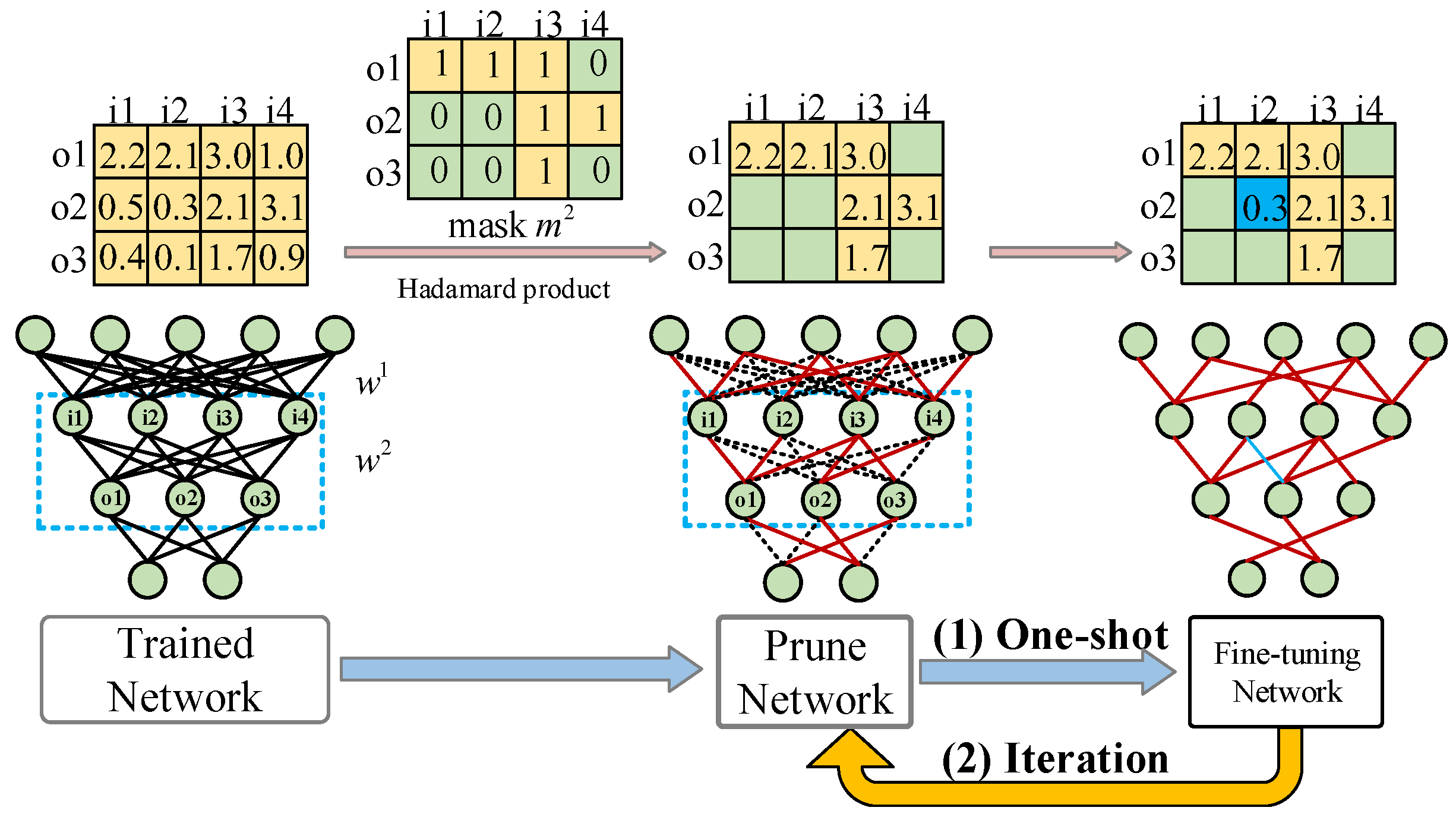
Neural network pruning is a classic technique in the model compression filed. As shown in Figure 3, network pruning requires a trained network, which is usually overparameterized. For a network N of depth L, the overall parameters contained can be obtained by $W=\left\{w^1,\dots ,w^L\right\}$, where $w^i$ denotes the parameter matrix of the i-th layer of the network.

Neural network pruning is usually achieved by pruning mask $M=\left\{m^1,\dots ,m^L\right\}$ [40]. $m_i$ represents the pruning mask of each layer of the network, which is usually represented by a binary matrix with the same dimension as $w_i$. Specifically, 0 means that the parameter is pruned and 1 means that the parameter is preserved. The pruned weight $w_{prun}^i$ is obtained by performing a Hadamard product on $m^i$ and $w^i$, and it can be expressed as $w_{prun}^i=w^i\odot m^i$. The process of neural network pruning is also shown in Figure 3.

Finally, the pruned network is fine-tuned. According to the pruning process, it can be divided into iterative pruning and one-shot pruning, the difference between the two pruning process is represented in Figure 3. Iterative pruning is a cyclical process of pruning and retraining, and many successful pruning methods [11,41,42] in the past have been based on iterative pruning. However, recent research [43,44] has suggested that such heavy consumption and the selection of design undermine their utility. One-shot pruning is trained after a one-time pruning process, and it can avoid the problem of iterative pruning.

2.3. Evolutionary Multi-Task Optimization

Evolutionary multi-task optimization (EMTO) [45,46,47,48,49] is an emerging paradigm in the field of evolutionary computation. By sharing searched knowledge in similar tasks, EMTO can improve the convergence characteristics and searching efficiency for each task [50]. As shown in Figure 4, EMTO randomly marks the individuals with different task cultures and maps them to the corresponding task space for evolving. Furthermore, the knowledge in each task is transferred by genetic material among individuals in a unified space. Furthermore, EMTO has been studied to solve similar tasks parallelly [51] and handling optimization problems efficiently by building module tasks [52,53,54,55]. In avoiding the possible negative transfer of knowledge, Gao et al. [56] reduced the divergence between subpopulations belonging to different tasks by aligning the distributions in the subspaces.

A minimization EMTO problem with K optimization tasks have a unified space $\Omega$. The j task, denoted as $T_j$, is considered to have a search space ${\Omega }_j$ on which the objective function $F_j:{\Omega }_j\to \Omega$ implements a mapping from subsearch space ${\Omega }_j$ to uniform space $\Omega$. In addition, each task may be constrained by several equality and/or inequality conditions that must be satisfied for a solution to be considered feasible. EMTO aims to optimize all tasks:

$$\begin{array}{c}\mathrm{minimize}\left\{F_1\left({\mathit{x}}_1\right),\cdots ,F_t\left({\mathit{x}}_t\right),\cdots ,F_k\left({\mathit{x}}_k\right)\right\}\hfill \end{array}$$

(1)

In evolutionary multi-task optimization, each individual is assigned a skill factor indicating the cultural trait of the associated task [51]. Then, the individuals are encoded in a unified search space and the genetic operators are applied to produce offspring in this space. The offspring also inherit the parents’ skill factors through the vertical cultural transmission.

2.4. Motivation

Deep neural networks achieve good classification results based on large-scale parameters. The complex nonlinear structure leads to complex calculation, which affects the application of neural network for HSI classification on mobile platforms. Therefore, it is necessary to compress the model of the existing large-scale network. Moreover, the training of neural networks relies on a large number of training samples. HSIs need to be manually labeled, so the labeled samples of HSIs are limited, which will lead to overfitting and classification difficulties during complex neural network training.

Traditional network pruning methods based on deep neural networks only deal with one image at a time, which has limited learning knowledge and does not make full use of the common features between similar images. The multi-task framework can be used to simultaneously prune the classification networks of multiple different images.Taking advantage of the potential similarities between optimization tasks, the multi-task framework can be used to simultaneously prune the classification networks of multiple different images. Using existing HSI with high similarity, when the same network architecture is trained on different datasets, its parameters characterize different datasets, so interaction between tasks can alleviate the limited sample problem on a single dataset and help the classification of the respective task. Although the existing evolutionary pruning methods can avoid the cost and prior knowledge requirements of designing pruning rules, they are difficult to optimize when facing more complex network structures. The proposed multi-task optimization framework, using knowledge transfer between tasks, can also effectively facilitate the respective optimization tasks.

3. Methodology

This section provides a comprehensive description of the proposed network collaborative pruning method for HSI classification. Firstly, the overall framework of the method is introduced. Secondly, compression of the model is achieved by an evolutionary multi-task pruning algorithm, the algorithm is introduced, and the initialization of individual and population, genetic operators, and self-adaptive knowledge transfer strategy are described in detail. Finally, the complexity of the proposed method is calculated.

3.1. The Framework of the Proposed Network Collaborative Pruning Method for HSI Classification

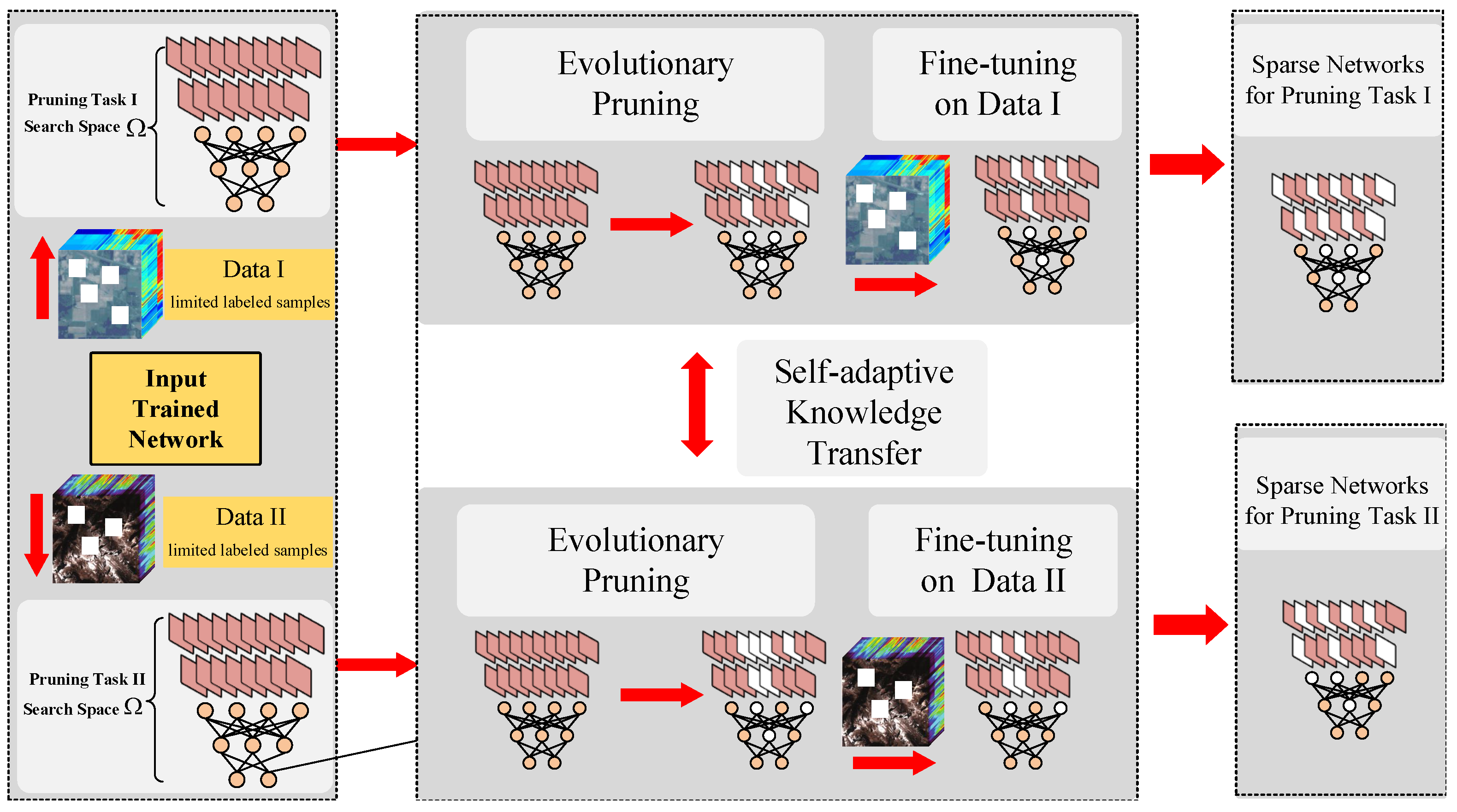
The overall framework of the proposed method is shown in Figure 5. First, different optimization tasks are constructed for two similar HSIs, i.e., there is a similarity between the two sparsification tasks. The evolutionary algorithm is used to search the potential excellent sparse network structure on the respective HSI. Genetic operators are designed according to the representation of the network structure. In the process of the parallel optimization of two tasks, interaction between tasks is needed to transfer the local sparse network structure. At the same time, in order to avoid the possible negative transfer, the self-adaptive knowledge transfer strategy is used to control the interaction strength between tasks. After completing the pruning search in different tasks and fine-tuning on the respective HSI, a set of sparse networks is obtained.

3.2. Evolutionary Multi-Task Pruning Algorithm

3.2.1. Mathematical Models of Multi-Tasks

In the evolutionary pruning algorithm, modeling is performed on different HSIs and the similarity between images is high. Therefore, the models of multi-tasks are given in (2).

$$\left\{\begin{array}{c}{T}_I=max(f_{acc}\left(W_{taskI}\right),f_{spar}\left(W_{taskI}\right))W_{taskI}\in \Omega \hfill \\ T_{II}=max(f_{acc}\left(W_{taskII}\right),f_{spar}\left(W_{taskII}\right))W_{taskII}\in \Omega \hfill \end{array}\right.$$

(2)

$$\left\{\begin{array}{c}{f}_{acc}\left(W_{prun}\right)=1-eval(D_{test},W_{prun})\hfill \\ f_{spar}(W,W_{prun})=\frac{{∥{\sum }_{i=1}^L{w}_{prun}^i∥}_{l0}}{\left|{\sum }_{i=1}^L{w}^i\right|}\hfill \end{array}\right.$$

(3)

where $T_I$ represents the classification and structure sparsification task on a certain HSI and the search space of $T_I$ is $\Omega$. Furthermore, the optimization of the task is achieved by searching the result pruned network weights $W_{taskI}$. Similarly, $T_{II}$ represents the classification and structure sparsification task on a different HSI, the search space of $T_{II}$ is also $\Omega$, and the pruned network weights obtained by searching is $W_{taskII}$.

Each task is a multi-objective optimization model which can be expressed by (3). Generally speaking, in the search process, when the network sparsity is reduced, the accuracy of the network will reduce; sparsity and accuracy are two conflicting goals. One objective function $f_{acc}$ represents the accuracy of the neural network on the test dataset $D_{test}$, and another objective function $f_{spar}$ represents the sparsity of the network, which can be represented by the pruning rate of the network. Specifically, sparsity can be expressed as the ratio of the number of all elements that are not zero to the number of all elements.

3.2.2. Overall Framework of Proposed Evolutionary Multi-Task Pruning Algorithm

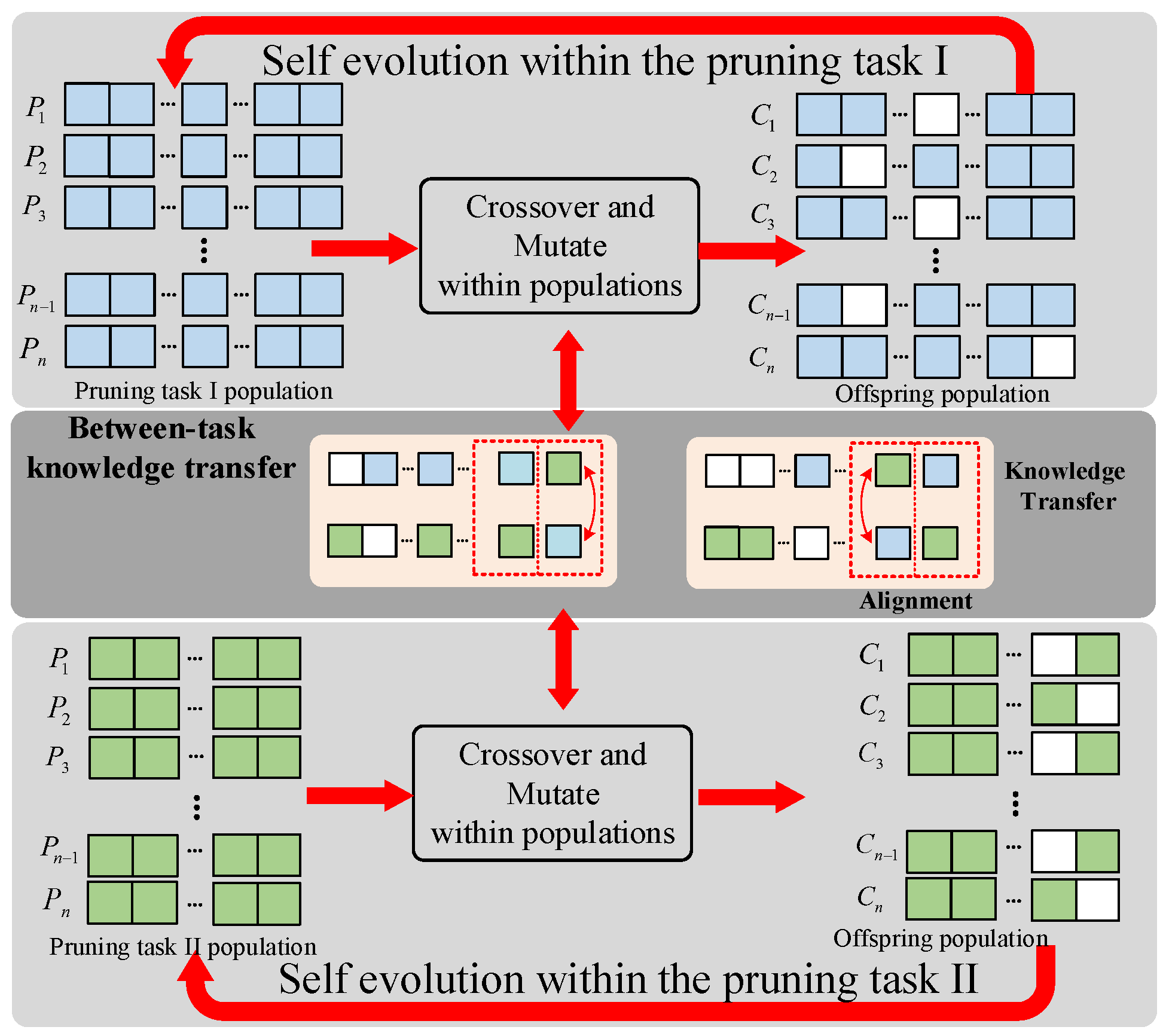
The evolutionary pruning algorithm is shown in Figure 6. One-dimensional vectors are designed for different tasks to represent different pruning schemes, which can also be regarded as a set of sparse networks. In these two optimization tasks, the stepwise optimization of the network structure within the task is achieved. Through the knowledge transfer between different tasks, the optimization efficiency of the two tasks is further improved. After the evolution is completed, a set of network pruning schemes that can balance accuracy and sparsity are obtained. The specific implementation of the evolutionary pruning algorithm based on multi-task parallel optimization is shown in Algorithm 1.

Algorithm 1 The proposed evolutionary multi-task pruning algorithm

Input: $pop$: task population size, t: number of evolutionary iterations, P: parent population,     $rmp$: random mating probability, $gen$: maximum number of generation Output: a set of trade-off sparse networks for multiple HSIs 1: Step (1) Train a state-of-the-art network N 2: Step (2) Construct task $T_I$ and task $T_{II}$ in $\Omega$ 3: Step (3) Pruning 4:    Set $t=1$ then initialize the population $P_t$ 5:   while ($t<gen$) do 6:     $P_t$← Binary Tournament Selection ($P_t$) 7:     Generate offspring $C_t$→ Refer Algorithm 2 8:     $R_t=C_t\cup P_t$ 9:     Update scalar fitness in $R_t$ 10:     Select $pop$ fittest members from $R_t$ to form $P_{t+1}$ by NSGA-II 11:     Self-adaptively update $rmp$→ Refer Algorithm 3 12:     $t=t+1$ 13:   end while 14: Step (4) Fine-tuning the optimized results in $T_I$ and task $T_{II}$

3.2.3. Representation and Initialization

In this paper, we adopt a one-dimensional vector to represent a layer-by-layer differentiated pruning scheme, which can also represent a unique sparse network. This can more comprehensively reflect the sensitivity differences of different layers in the neural network, so as to achieve more refined and differentiated pruning. This encoding method can be well extended to a variety of networks, only needing to determine the depth of the network to achieve encoding and pruning. On the other hand, the use of one-dimensional vector encoding makes the design of genetic operators more convenient. Each element in the vector represents the weight pruning ratio of each layer of the network, which is the proportion of 0 elements in the $w_i$ matrix. Thus, the encoding vector of layer i can be represented by the $w^i$ as:

$$\begin{array}{c}vector\left[i\right]=\frac{{∥w^i∥}_{l0}}{\left|w^i\right|}\hfill \end{array}$$

(4)

Similar to (3), ${∥w^i∥}_{l0}$ represents the number of nonzero elements in the layer i, and $\left|w^i\right|$ represents the number of elements in this layer. In the pruning process, the weights are sorted from small to large according to the element value of the i-th bit of the one-dimensional vector, and the weight of the former $vector\left[i\right]\%$ is pruned. The upper and lower bounds of $vector\left[i\right]$ are 0 and 1, respectively. In this way, the network weights are pruned layer by layer, and the sparse network structure corresponding to the one-dimensional vector can be finally obtained. The search process tries to approach the real Pareto-optimal front. The decoding operation is the reverse process of the encoding operation.

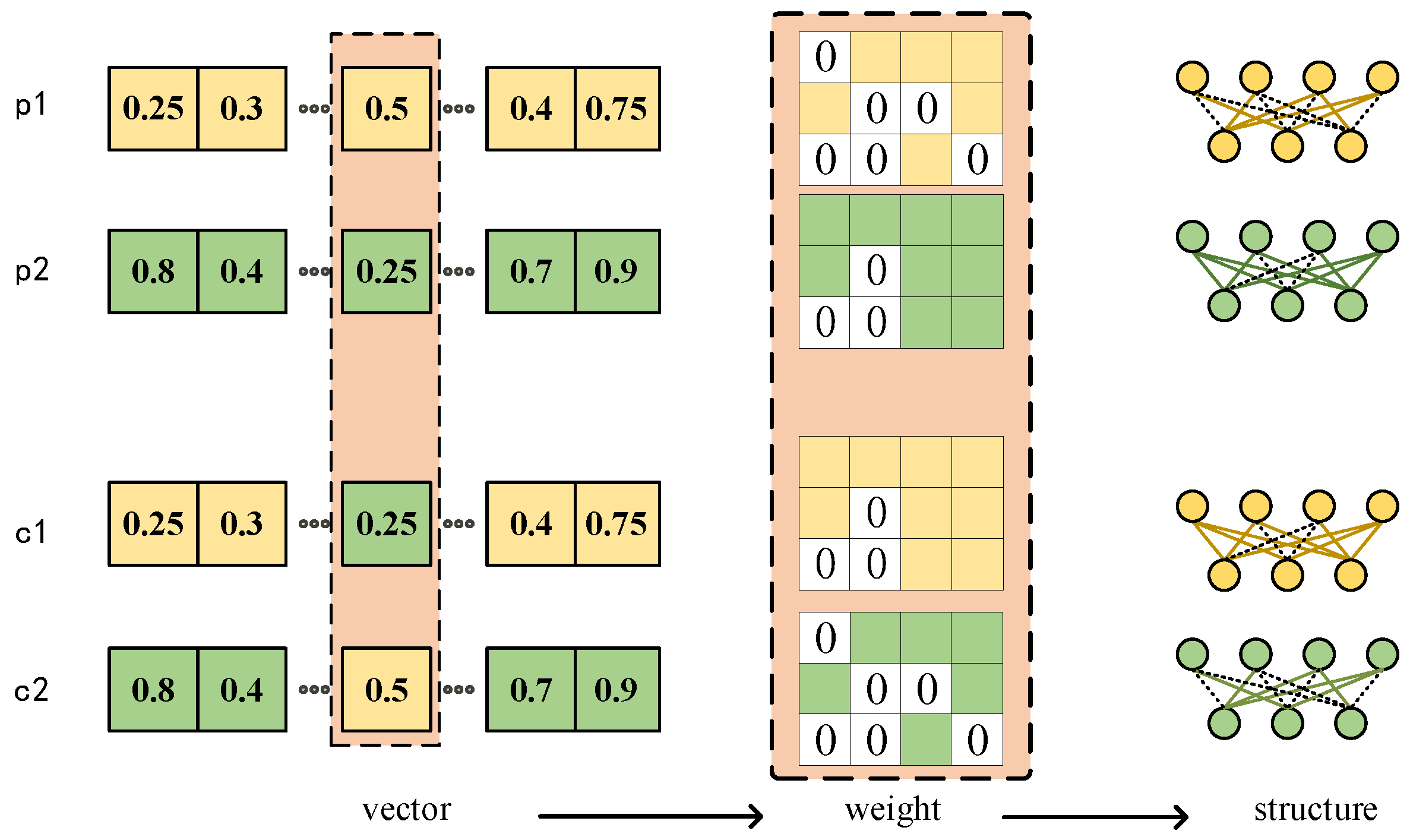
Specifically, as shown in Figure 7, for a pruning scheme, its i-th element is a and its j-th element is b. Firstly, the weights of layers i and j are arranged from small to large. Suppose that pruning $a\times 100\%$ of the weights in the i-th convolution layer, the total parameter $\left|w^i\right|$ of this layer is $k_w^i\times k_h^i\times f^i$, where $k_h^i$ represents the height of the convolution kernel, $k_w^i$ represents the width of the convolution kernel, $f^i$ represents the number of convolution filters in this layer. Suppose that pruning $b\times 100\%$ of the weights in the j-th fully connected layer, the total parameter $\left|w^j\right|$ is the product of the input neurons $n_{in}^j$ and output neurons $n_{out}^j$. After determining the pruned parameter, the corresponding bit is set to zero to indicate that the parameter is pruned.

According to the depth L of the network and the population size $pop$, $pop$ one-dimensional vectors of length L are randomly generated to form the initial population of task. This represents $pop$ pruning schemes, which can also be regarded as $pop$ different sparse networks. The population is initialized in the same way for different tasks.

3.2.4. Genetic Operator

The genetic operators used in proposed algorithm include crossover and mutation operators. It is necessary to judge the skill factor of the individual when two individuals crossover. This is similar to MFEA [45]. If two randomly selected parent pruning schemes have the same skill factor, they come from the same task and crossover directly. Otherwise, it comes from different tasks, and $rmp$ is needed to determine whether to carry out knowledge transfer between tasks. After completing the crossover operation, the individual performs the mutation operation. The generated offspring individuals inherit the skill factor of the parent individual. If within-task crossover is performed, the skill factor of the offspring is the same as that of the parents, otherwise, the offspring randomly inherits the skill factor of one parent. The details are shown in Algorithm 2.

Algorithm 2 Genetic operations

Input: $p_1,p_2$: candidate parent individuals, ${\tau }_i$: the skill factor of the parent, $rmp$: random     mating probability, $rand$: a random number between 0 and 1 Output: offspring individual $c_1,c_2$ 1: if ${\tau }_1=={\tau }_2$ then or $rand<rmp$ 2:     $c_1,c_2$← Crossover($p_1,p_2$) 3:     for $iselectfrom\{1,2\}$ do 4:         $c_i$← Mutate($p_i$) 5:     end for 6:     if ${\tau }_1=={\tau }_2$ then 7:         $c_i$ inherits the skill factor from $p_i$ 8:     else 9:         if $rand<0.5$ then 10:            $c_1,c_2$ inherits ${\tau }_1$ from $p_1$ 11:         else 12:            $c_1,c_2$ inherits ${\tau }_2$ from $p_2$ 13:         end if 14:     end if 15: else 16:     for $iselectfrom\{1,2\}$ do 17:         $c_i$← Mutate($p_i$) 18:         $c_i$ inherits the skill factor from $p_i$ 19:     end for 20: end if

Both between-task and within-task crossover operators are designed in the same single-point crossover. The i-th value in $vector$ of parents $p_1$ and $p_2$ are swapped to generate two new individuals $c_1$ and $c_2$. As shown in Figure 8, when individuals crossover at a certain bit, the bit on different individual vectors is swapped directly. Because pruning rate and sparse structure correspond one-to-one, it is also directly exchanged at the weight matrix of the network.

A polynomial-mutation [57] is designed when the crossover operation is complete. Figure 9 depicts the mechanism of the designed mutation operator. Taking individual $p1$ for example, the i-th value changes as preset mutate probability from 0 to 0.25, which can be calculated from the polynomial mutation in Figure 9. The change quantity ${\beta }_i$ in layer i is related to the $u_i\in [0,1)$ and the non-negative real number ${\eta }_u$. ${\eta }_u$ is the distribution exponent. The larger this value is, the more similar the offspring and the parent are, so ${\eta }_u=10$ is set as the mutation probability. There are four input neurons and three output neurons in this layer for a total of 12 weight parameters. During pruning, the weights are sorted, then select the weight from small to large for pruning, and the sparse structure obtained after mutation operation is unique. Therefore, a total of three bits in the matrix need to be changed.

The crossover and mutation operators adopted in this paper not only realize the self-evolution within tasks but also transfer the effective sparse structure so as to promote the search efficiency of two tasks.

3.2.5. Self-adaptive Knowledge Transfer Strategy

Although there is a high similarity between the two tasks [58], negative transfer is still inevitable; this affects the search efficiency and solution quality. So, a self-adaptive knowledge transfer strategy based on historical information and a dormancy mechanism is designed. The intensity of transfer can be adjusted adaptively by taking advantage of individual contributions. The dormancy mechanism is used to suppress irrelevant knowledge transfer, reduce the interference of useless knowledge to task search, and save computing resources.

Algorithm 3 introduces the self-adaptive knowledge transfer strategy. New individuals generated by knowledge transfer between tasks are labeled as $\left\{p_{tki}\right|i=1,2,\dots ,n\}$. After the fitness evaluation of the generated offspring, the Pareto rank of the offspring individual in the non-dominated ranking is obtained. The knowledge transfer contribution $TKCR$ can then be represented by the rank of the individual with the best non-dominated rank result among these newly generated individuals. Then, $TKCR$ controls the value of $rmp$. Notice that when comparing the Pareto rank of the offspring, the task to which the offspring belongs is not distinguished.

Algorithm 3 Self-adaptive knowledge transfer strategy

Input: $N_{p1},N_{p2}$: the population size in multi tasks, $ran{k}_{min}$: minimum rank of non-     dominated sort, $p_{tki}$: new individuals generated by knowledge transfer, $ϵ$: preset     threshold Output: random mating probability $rmp$ 1: $ran{k}_{min}\leftarrow {min}_{rank}(p_{tk1},p_{tk2},\dots ,p_{tkm})$ 2: $\delta \leftarrow ran{k}_{min}/(N_{p1}+N_{p2})$ 3: Transfer knowledge contribution $TKCR\leftarrow$$1-\delta$ 4: if $TKCR>ϵ$ then 5:     $rmp$$\leftarrow TKCR$ 6: else 7:     $rmp\leftarrow 0.1$ 8: end if

When the value of $TKCR$ is less than the set threshold $ϵ$ of population interaction, the dormancy condition of the population is reached, and $rmp$ is set to a small fixed value. When the value of $TKCR$ is greater than $ϵ$, the transfer of useful knowledge is detected at this time, the self-adaptive update is resumed, and then, the value of $rmp$ is the value of $TKCR$. Through the self-adaptive strategy to control the frequency of knowledge transfer in the evolution process and the dormancy mechanism, the impact of negative transfer between tasks on task performance can be effectively avoided.

3.3. Fine-Tune Pruned Neural Networks

After pruning, a set of sparse networks is obtained. Then, they are retrained, as studied in [59]. In detail, these networks are trained with the Adam optimizer, and the initial learning rate, weight decay, and training epochs are set differently according to different data. The learning rate is adjusted by cosine annealing with the default setting.

3.4. Computational Complexity of Proposed Method

An analysis of the computational complexity of the proposed method is calculated in two parts: the computational cost of evolutionary computation and the computational cost of fine-tuning. In the pruning parts, the computational complexity is $O\left(GPC\right)$, where G is the number of generations, P is the number of individuals, and C is the cost of given function. Assuming the computational cost of training for each epoch is $O\left(T\right)$, the fine-tuning computational complexity is $O\left(ET\right)$, E denotes the number of training epochs. Therefore, the computational complexity of the proposed approach is $O(GPC+PTE)$. Because the proposed method is multi-task optimization and is able to handle two HSIs pruning tasks simultaneously, it is twice the computational complexity of a single evolution and fine-tuning process.

4. Experiments

In this part, experiments that are carried out on HSIs to verify the effectiveness of the proposed method are described. Firstly, it is verified that the pruned network has better classification accuracy with limited labeled samples on multiple HSIs. The proposed method is compared with other neural network pruning methods, and the relevant parameters of the pruned network are compared with other methods. After that, the sparse networks obtained on the Pareto-optimal front are compared to prove the effectiveness of the multi-objective optimization. The effectiveness of the proposed self-adaptive knowledge transfer strategy is proven by quantifying the knowledge transfer between tasks. Finally, the proposed method is validated on more complex networks and larger HSI.

4.1. Experimental Setting

A 3DCNN [36] trained on the HSI was used to validate proposed method. The structure of network is composed of convolutional layers of different stride. The convolutional layer with stride 1 is called Conv, and the convolutional layer with stride 2 is called ConvPool. Excluding the classification layer, the number in the network structure is the number of the filter of the convolutional layer, and the network structure can be expressed as: 3DConv(20)-1DConvPool(2)- 3DConv(35)- 1DConvPool(2)-3DConv(35)- 1DConvPool(2)-3DConv(35)-1DConvPool(35)-1DConv(35)-1DconvPool(35).

HSIs use Indian Pines, Salinas, and University of Pavia datasets. Data in the real world not only have the problem of limited labeled samples, but also the labeled samples often cannot reflect the real distribution of the data. For example, only part of the HSI in a certain area of the ground are sampled in the detection, and these data are continuous but may not be comprehensive. In order to simulate limited sample data, 10% labeled samples were set for each dataset, and the sample of the corresponding comparison methods was also 10%.

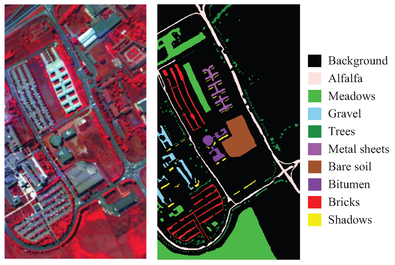
The Indian Pines (IP) dataset is collected by the sensor AVIRIS [60] from a pine forest test site in northwest India. Its wavelength range is 400–2500 nm. After removing the water absorption area, there are 200 spectral segments in total, and the spatial image size of each spectral segment is $145\times 145$, with a total of 16 types of labels. The spatial resolution of this dataset is only 20 m. Figure 10 shows the pseudo-color plots and labels of Indian Pines.

The Salinas (SA) dataset is collected from the Salinas Valley in California by the sensor AVIRIS. After removing the water absorption area, there are a total of 200 spectral segments, and the spatial image size of each spectral segment is $521\times 217$, with a total of 16 labels. The spatial resolution of this dataset is 3.7 m. Figure 11 show the pseudo-color plots and labels of Salinas.

The University of Pavia (PU) dataset is collected by the sensor ROSIS near the University of Pavia, Italy. After removing the water absorption area, there are a total of 103 spectral segments, and the spatial image size of each spectral segment is $610\times 340$, with a total of nine categories of labels. The spatial resolution of this dataset is 1.3 m. Figure 12 shows the pseudo-color plot and labels of the University of Pavia.

The proposed method was compared with five deep learning methods, including 1DCNN [61], 3DCNN [62], M3DCNN [63], DCCN [64], HybridSN [65], ResNet [66], and DPRN [67]. In the experiment, three evaluation metrics—overall accuracy ($\mathrm{OA}$), average accuracy ($\mathrm{AA}$), and Kappa coefficient ($\kappa$)—were used to evaluate the classification effect of the proposed method. The parameters of our proposed method are shown in

Table 1. Parameters used in proposed method.

	HSI Datasets
Offspring size in pruning task I	50
Offspring size in pruning task II	50
Maximum number of generation	50
Mutation probability	10
Crossover probability	10
The initial value of transfer	0.5
The dormancy condition	0.1

.

The experimental server included four Intel(R) Xeon(R) Silver 4214R cpus @ 2.40 GHz, 192 GB DDR4 RAM, Two NVIDIA Tesla K40 12 GB Gpus and eight NVIDIA Tesla v1000s Gpus were used. The software environment used the Ubuntu operating system with Pytorch framework and Python 3.6 as the programming language. The optimizer of the convolutional neural network was set to Adam optimizer, the weight decay was 0, betas = (0.9, 0.999), and eps = $1\times {10}^{-8}$. The initial learning rate was $1\times {10}^{-4}$, the learning rate decay was adopted by cosine annealing, the number of training epochs of the network was 200, and the batch size was 100.

4.2. Results on HSIs

4.2.1. Classification Results

In the experiment, two groups of experiments were constructed to analyze the influence on the performance of the proposed method. The first group uses the Indian Pines dataset and the Salinas dataset, and the second group uses the University of Pavia dataset and the Salinas dataset. The Indian Pines dataset and Salinas dataset are from the same sensor, and the University of Pavia dataset and Salinas dataset are from different sensors.

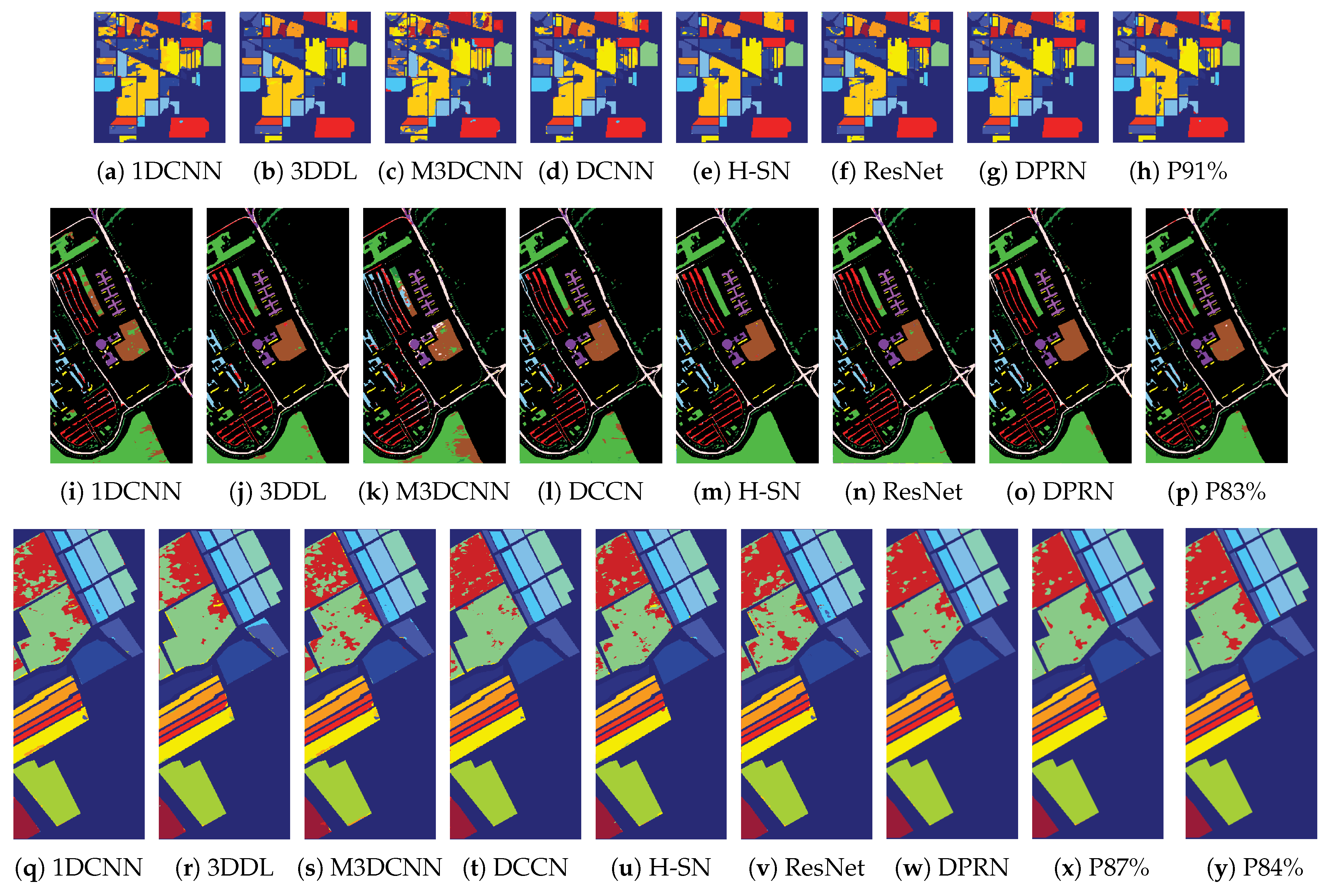
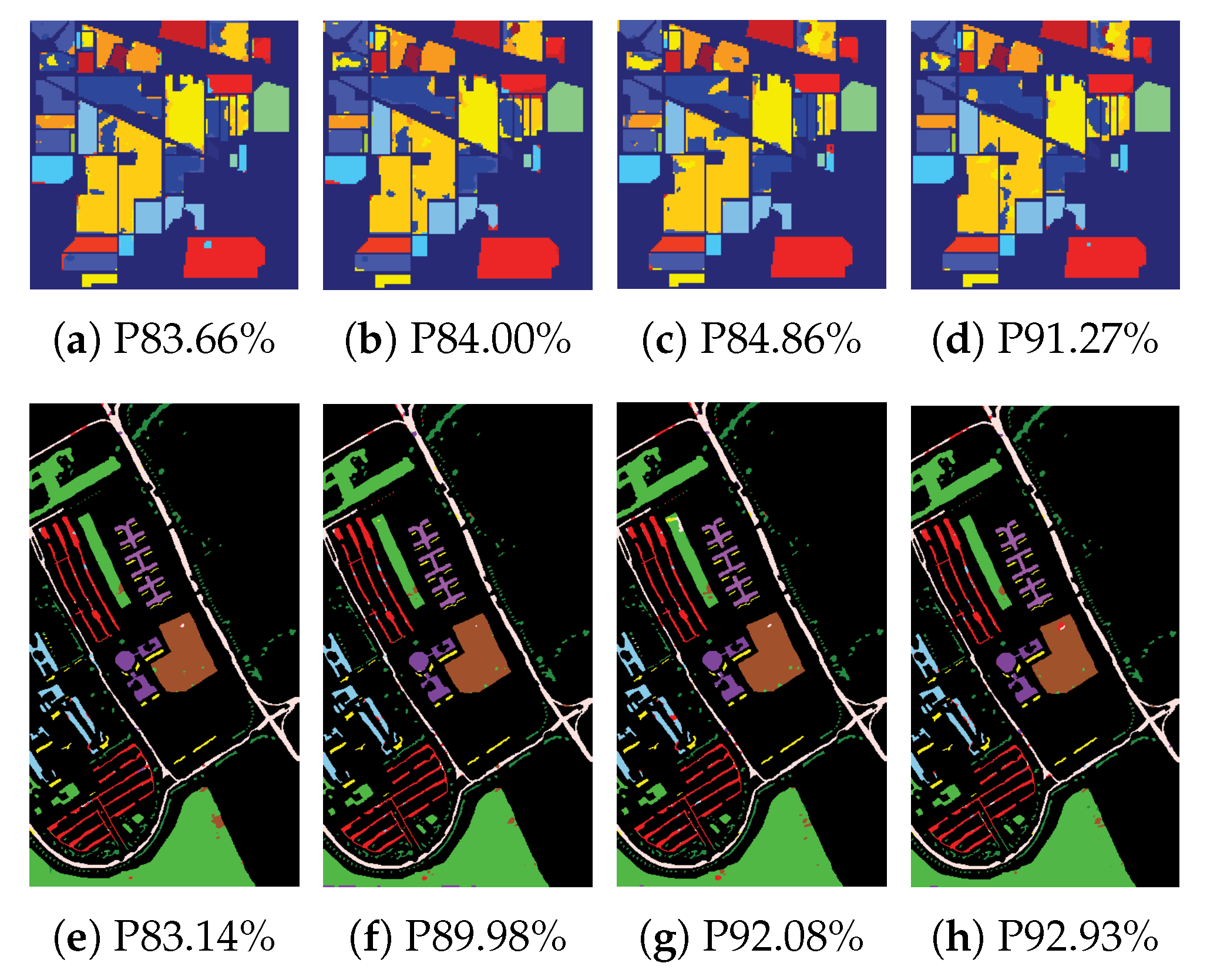
The classification result of the Indian Pines dataset is shown in Figure 13, and the specific classification result table is shown in

Table 2. Classification accuracy (%) for the collaborative pruning task (Indian Pines and Salinas). Best results are reported in bold.

Category	1DCNN	3DDL	M3DCNN	DCCN	HybridSN	ResNet	DPRN	Pruned 87.15%
OA (%)	91.78 ± 1.45	92.05 ± 1.37	90.51 ± 0.98	95.66 ± 2.06	91.68 ± 1.71	93.68 ± 1.03	97.14 ± 0.77	95.70 ± 1.31
AA (%)	96.13 ± 2.33	95.50 ± 2.67	95.41 ± 2.56	98.05 ± 0.42	96.10 ± 2.11	97.46 ± 1.68	98.59 ± 1.09	98.14 ± 0.69
Kappa (%)	90.87 ± 2.06	91.13 ± 2.01	89.45 ± 2.79	95.17 ± 1.78	90.77 ± 2.21	92.99 ± 1.51	96.10 ± 0.68	95.14 ± 0.74
1	99.95	99.90	99.70	98.45	98.35	99.75	99.10	99.70
2	99.59	99.81	99.27	99.78	99.81	100.00	99.88	100.00
3	98.93	86.33	97.36	99.84	98.27	99.39	100.00	99.24
4	99.78	99.92	99.28	98.78	99.71	99.85	99.03	99.07
5	98.39	98.99	99.62	100.00	96.34	98.80	99.49	99.03
6	99.99	99.99	99.98	99.99	99.99	100.00	100.00	99.97
7	99.52	99.30	99.46	99.94	99.49	99.97	99.81	99.47
8	80.09	88.59	77.82	85.04	76.69	78.79	93.17	88.31
9	99.06	99.64	98.37	99.91	98.59	99.48	99.82	99.77
10	90.69	95.21	91.03	96.06	93.47	97.98	98.42	98.26
11	99.06	99.90	99.25	99.06	98.68	99.06	100.00	99.34
12	99.01	97.76	99.01	100.00	98.96	99.89	99.71	99.95
13	99.34	99.45	99.23	99.01	98.79	100.00	100.00	100.00
14	99.06	97.38	97.75	99.34	98.69	98.31	99.55	100.00
15	77.06	66.82	72.45	94.04	81.89	88.44	89.32	88.37
16	98.61	99.00	96.90	99.50	99.88	99.61	99.74	99.89
Category	1DCNN	3DDL	M3DCNN	DCNN	HybridSN	ResNet	DPRN	Pruned 91.27%
OA (%)	80.93 ± 4.37	91.45 ± 3.62	95.18 ± 3.74	92.17 ± 3.79	95.38 ± 2.91	93.24 ± 2.86	97.46 ± 1.50	88.90 ± 1.27
AA (%)	90.15 ± 3.77	96.84 ± 2.81	98.07 ± 1.72	93.45 ± 2.26	98.12 ± 0.58	97.89 ± 1.43	98.05 ± 0.49	95.38 ± 0.81
Kappa (%)	78.38 ± 4.69	90.33 ± 2.84	94.52 ± 2.94	91.11 ± 3.19	94.75 ± 1.67	93.11 ± 2.48	95.97 ± 1.39	87.46 ± 0.93
1	100.00	100.00	100.00	100.00	100.00	100.00	100.00	100.00
2	65.68	96.42	93.20	82.56	89.28	91.75	96.68	76.96
3	73.97	96.14	97.34	91.20	97.22	96.26	98.23	95.66
4	100.00	100.00	100.00	95.78	100.00	100.00	100.00	100.00
5	96.48	100.00	100.00	96.27	99.17	100.00	100.00	99.37
6	99.31	99.86	99.45	98.63	99.86	100.00	100.00	98.35
7	100.00	100.00	100.00	92.86	100.00	100.00	100.00	100.00
8	100.00	100.00	100.00	100.00	100.00	100.00	100.00	100.00
9	100.00	100.00	100.00	90.00	100.00	100.00	100.00	100.00
10	64.19	88.58	93.10	91.67	100.00	93.18	97.48	91.15
11	72.66	73.28	88.55	91.57	97.42	81.92	93.74	76.65
12	75.71	97.97	98.65	86.34	90.17	97.95	99.03	92.91
13	100.00	100.00	100.00	100.00	98.14	100.00	100.00	100.00
14	95.25	99.84	98.81	97.00	100.00	98.37	99.28	95.81
15	99.22	97.40	100.00	95.34	98.89	100.00	100.00	99.22
16	100.00	100.00	100.00	86.02	99.74	100.00	100.00	100.00

. Although the pruned network do not obtain the best results on the three evaluation metrics, it obtain the highest classification accuracy on the seven categories, all of which are 100%. The network for Indian pines dataset is able to prune 91.2% of the parameters.

From the overall evaluation metrics, it can be seen that when the Indian Pines dataset from the same sensor is used as an another task, it obtains relatively better results, and pruning 87.2% of the network weights. By transferring the existing knowledge, the method successfully improves the classification accuracy of the network and greatly reduces the complexity of the network model. It is basically superior to other deep learning methods in the $\mathrm{OA}$ and $\mathrm{AA}$. Although the number of samples in each category of data is not balanced, the knowledge transfer can improve the overall performance of the sparse network, so that the network still achieves a high $\kappa$, that is, the distribution of classification accuracy on each category is balanced.

The classification result of the University of Pavia dataset is shown in Figure 13, and the specific classification results are shown in

Table 3. Classification accuracy (%) for the collaborative pruning task (University of Pavia and Salinas). Best result are reported in bold.

Category	1DCNN	3DDL	M3DCNN	DCCN	HybridSN	ResNet	DPRN	Pruned 84.30%
OA (%)	91.78 ± 1.45	92.05 ± 1.37	90.51 ± 0.98	95.66 ± 2.06	91.68 ± 1.71	93.68 ± 1.03	97.14 ± 0.77	95.02 ± 0.98
AA (%)	96.13 ± 2.33	95.50 ± 2.67	95.41 ± 2.56	98.05 ± 0.42	96.10 ± 2.11	97.46 ± 1.68	98.59 ± 1.09	98.03 ± 0.30
Kappa (%)	90.87 ± 2.06	91.13 ± 2.01	89.45 ± 2.79	95.17 ± 1.78	90.77 ± 2.21	92.99 ± 1.51	96.10 ± 0.68	94.03 ± 1.12
1	99.95	99.90	99.70	98.45	98.35	99.75	99.10	99.60
2	99.59	99.81	99.27	99.78	99.81	100.00	99.88	99.97
3	98.93	86.33	97.36	99.84	98.27	99.39	100.00	99.60
4	99.78	99.92	99.28	98.78	99.71	99.85	99.03	99.28
5	98.39	98.99	99.62	100.00	96.34	98.80	99.49	99.44
6	99.99	99.99	99.98	99.99	99.99	100.00	100.00	99.97
7	99.52	99.30	99.46	99.94	99.49	99.97	99.81	99.66
8	80.09	88.59	77.82	85.04	76.69	78.79	93.17	84.86
9	99.06	99.64	98.37	99.91	98.59	99.48	99.82	99.97
10	90.69	95.21	91.03	96.06	93.47	97.98	98.42	98.14
11	99.06	99.90	99.25	99.06	98.68	99.06	100.00	100.00
12	99.01	97.76	99.01	100.00	98.96	99.89	99.71	99.95
13	99.34	99.45	99.23	99.01	98.79	100.00	100.00	100.00
14	99.06	97.38	97.75	99.34	98.69	98.31	99.55	99.91
15	77.06	66.82	72.45	94.04	81.89	88.44	89.32	88.06
16	98.61	99.00	96.90	99.50	99.88	99.61	99.74	100.00
Category	1DCNN	3DDL	M3DCNN	DCCN	HybridSN	ResNet	DPRN	Pruned 83.14%
OA (%)	88.32 ± 3.76	81.67 ± 3.17	94.36 ± 1.43	97.43 ± 1.12	93.47 ± 1.69	97.72 ± 1.19	98.48 ± 0.86	97.57 ± 1.40
AA (%)	91.29 ± 2.86	85.11 ± 3.84	94.87 ± 2.77	96.12 ± 2.01	94.81 ± 2.17	97.14 ± 1.28	98.36 ± 0.92	97.84 ± 0.95
Kappa (%)	84.85 ± 3.21	76.24 ± 3.65	92.59 ± 1.79	96.60 ± 2.24	91.46 ± 2.60	96.91 ± 1.28	97.19 ± 1.06	96.79 ± 0.69
1	83.47	69.91	85.03	95.53	86.98	92.35	94.12	95.58
2	87.08	82.99	96.24	99.52	93.71	98.92	99.48	98.14
3	88.42	74.08	89.09	88.61	88.58	95.41	96.86	96.95
4	96.57	94.48	96.34	96.01	96.96	96.99	97.94	97.74
5	99.99	99.95	99.99	100.00	99.99	100.00	100.00	99.77
6	91.05	72.51	98.03	98.01	97.43	99.97	99.63	98.60
7	91.42	83.75	95.78	97.66	96.76	98.84	99.60	99.92
8	84.46	90.82	94.16	95.54	93.18	97.48	94.41	95.05
9	99.15	97.57	99.15	94.19	99.47	99.62	99.52	98.83

. It can be seen that although 83.1% of the parameters are pruned, the pruned network still obtains high $\mathrm{OA}$, $\mathrm{AA}$, and $\kappa$ values, which are 97.57%, 97.84%, and 96.79%, respectively. In addition to this, the best results are achieved in three categories. This proves that leveraging the knowledge transferred from other images can facilitate the training of the network on the current image.

Sub-optimal results were obtained on the different sensor University of Pavia dataset, which still has certain advantages compared with other deep learning methods. Using the University of Pavia dataset as another task, 84.3% of network parameters were pruned. Compared with the results on the Indian Pines dataset, the number of retained parameters is greater, and the classification performance and consistency are lower.

These two groups of experiments show that the search efficiency of task can be promoted by transferring the important sparse structure of the SOTA network from the another task. In view of the differences between the two groups of experiments due to the same physical imaging logic under the same sensor device the similarity between the datasets is higher, and the spectral features are more common, so the better results can be achieved. Due to the lack of labeled training samples and the high complexity of the network model, the parameters are too large, so the evaluation metrics of the unpruned neural network is low, which reflects the limitation of the lack of labeled samples on the network training.

4.2.2. Comparison with other Neural Network Pruning Methods

The proposed method was compared to three neural network pruning methods in

Table 4. Classification results of the networks obtained by different pruning methods on the three HSIs. Best result are reported in bold.

HSI	Method	L2Norm	MOPSO	LAMP	NCPM
Salinas	Pruned (%)	87.00	85.24	87.00	87.15
	OA (%)	86.66	90.40	94.28	95.02
	AA (%)	91.48	94.65	97.68	98.03
	Kappa (%)	85.24	89.31	93.64	94.03
Indian Pines	Pruned (%)	91.00	90.23	91.00	91.27
	OA (%)	66.49	72.68	89.31	88.90
	AA (%)	81.44	84.61	94.90	95.38
	Kappa (%)	62.52	69.23	87.90	87.46
University of Pavia	Pruned (%)	83.00	84.11	83.00	83.14
	OA (%)	87.03	90.67	96.86	97.57
	AA (%)	87.4	87.70	97.54	97.84
	Kappa (%)	83.1	87.51	95.87	96.79

. NCPM is the network collaborative pruning method proposed in this paper. Because NCPM is a multi-objective optimization method, it selects a sparse network on the Pareto-optimal front.

The first pruning method L2Norm [68] is based on L2 norm, which sets a threshold for pruning for each layer by comparing the weight value of network parameters in each layer. In addition, NCPM is compared with MOPSO [21], a method based on particle swarm optimization. LAMP [12] is an iterative pruning method. LAMP utilizes a layer-adaptive global pruning importance score for pruning.

The three comparison methods and the proposed method all use the 3D-DL network. The original three pruning methods are all proposed based on 2DCNN and are suitable for image classification datasets, such as MNIST and CIFAR10. Therefore, the original pruning method needs to be changed to the pruning of 3DCNN. When training the network model, the same experimental settings such as the optimizer and learning rate are used as in NCPM.

NCPM obtains the best pruning results on Salinas and University of Pavia, and the OA of the pruned network is much better than that of L2Norm and MOPSO with the same pruning rate. The pruned network on Indian Pines is highly similar to the LAMP method, but both are better than L2Norm and MOPSO.

From the three HSIs, it can be clearly seen that the sparse network searched by the L2Norm is sub-optimal due to the single redundancy evaluation criterion, and the evolutionary pruning method can search a better sparse network structure. Due to the lack of diversity in selecting solutions, the sparse network searched by MOPSO is inferior to the NCPM method. The LAMP method is an iterative pruning method, and it will be retrained in an iteration process, which will cause additional computational complexity.

Compared with other pruning methods, NCPM can simultaneously prune two hyperspectral data classification networks, which improves the search efficiency. At the same time, the multi-objective optimization of the sparsity and accuracy of the network structure can obtain a set of sparse networks after one run.

4.2.3. Complexity Results of the Pruned Network

Table 5. Comparison results of the complexity of the pruned network.

HSIs	Methods	1DCNN	M3DCNN	HybridSN	ResNet	3DDL	Pruned
Indian pines	EpochTrainTime/s	40.5771	49.8241	73.0636	67.3195	60.1175	60.4814
	Parameter	246,409	263,584	534,656	414,333	259,864	22,868
	OA (%)	80.93	95.18	95.38	93.24	91.45	88.90
Pavia University	EpochTrainTime/s	40.3595	43.3423	79.7415	56.5454	41.6149	34.0278
	Parameter	246,409	263,584	534,656	534,656	259,864	43,918
	OA (%)	88.32	94.36	93.47	97.50	81.67	95.02
Salinas	EpochTrainTime/s	64.9641	85.6064	173.6447	134.5664	68.5989	65.7300
	Parameter	246,409	263,584	534,656	534,656	259,864	33,262
	OA (%)	91.78	90.51	91.68	93.68	92.05	95.70

shows the comparison results between the pruned network and the original network, as well as other neural networks, where the training time refers to a training time of 200 epochs. Our method is able to prune the 3D-DL network, and when compared with the original network, 3D-DL, the pruned network can cut most of the parameters and can also accelerate the test time of the network in a certain range. On the Univeristy of Pavia dataset, the training time was reduced by 18.23%, on the Salinas dataset, the training time was reduced by 4.18%, and on the Indian Pines, the time was almost unchanged. The pruned network achieves the best results when compared to other methods the Indian Pines and University of Pavia datasets. The comparison experiment proves the significance and necessity of neural network pruning.

4.2.4. The Result of the Sparse Networks Obtained by Multi-Objective Optimization

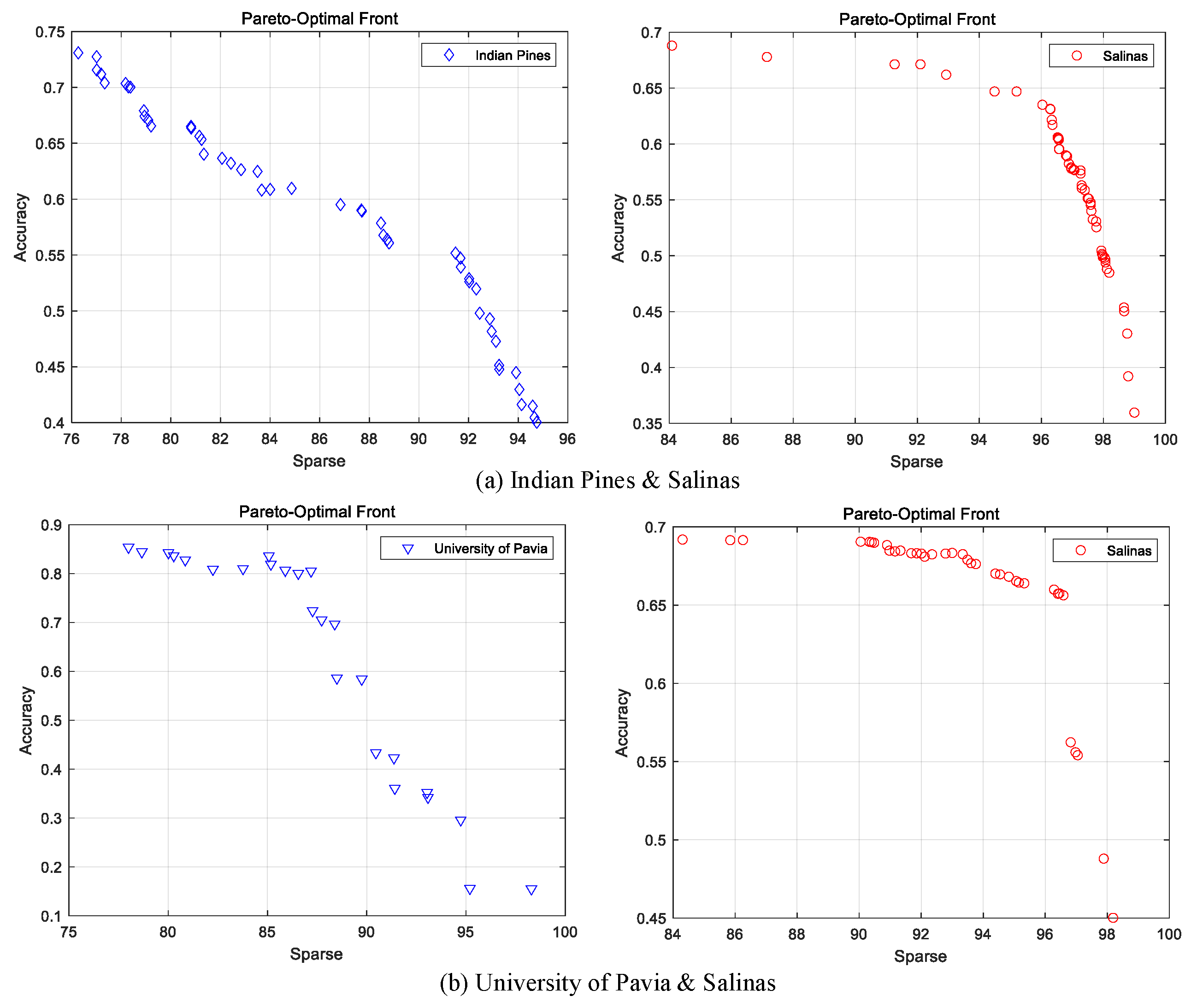
Figure 14 represents the Pareto-optimal front without fine-tuning in both two experiments. The Pareto-optimal front obtained for the Indian Pines dataset is uniformly distributed, whereas the Pareto-optimal front obtained for the University of Pavia is sparsely distributed. For the comparison of the Salinas dataset Pareto-optimal front in different experiments, the diversity of solutions is better in the multi-task optimization experiment of the Indian Pines dataset with the same sensor.

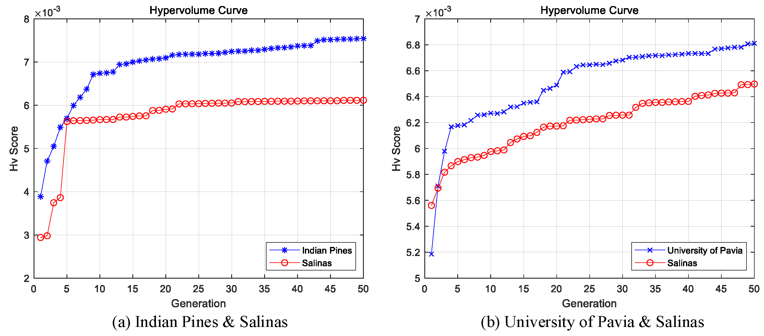
The hypervolume curve Figure 15 is used to represent the convergence of the evolutionary search process. The hypervolume of each generation is determined by the sparse network on the Pareto-optimal front, and the diversity and quality of the sparse network affect the hypervolume. The initialization of the two experiments is random, so the initial $hv$ is different. By comparing the results on the Salinas dataset in different experiments, it can be seen that the Salinas hypervolume curve optimized by the Indian Pines multi-task optimization converges faster and improves more, which again verifies the influence of the similarity between tasks on the results of multi-task optimization. In addition, the growth trend of the $hvscore$ is the same in the two sets of experiments, and the period of faster growth of $hvscore$ coincides, which can be understood as the promotion effect of knowledge transfer between the two tasks for their respective tasks.

Four networks on the Indian Pines dataset were selected for comparison with the original unpruned network in

Table 6. Results after fine-tuning sparse networks on the Pareto-optimal front on collaborative pruning task (Indian Pines and Salinas). Best results are reported in bold.

Category	ORG	Pruned Networks in Salinas					Category	ORG	Pruned Networks in Indian Pines
Pruned (%)	0.00	84.09	87.15	92.93	96.49	97.21	Pruned (%)	0.00	83.66	84.00	84.86	91.27
OA (%)	92.05	95.25	95.70	95.42	95.51	95.42	OA (%)	91.45	89.75	89.87	89.64	88.90
KAPPA (%)	91.13	94.72	95.22	94.90	95.01	94.90	KAPPA (%)	90.33	88.39	88.52	88.29	87.46
AA (%)	95.50	97.97	98.14	97.96	97.98	97.83	AA (%)	96.84	95.02	94.85	95.02	95.38
1	99.90	99.55	99.70	100.00	99.65	99.65	1	100.00	100.00	100.00	100.00	100.00
2	99.81	99.75	100.00	100.00	100.00	99.86	2	96.42	88.16	79.20	83.89	76.96
3	86.33	99.24	99.24	98.83	99.03	98.07	3	96.14	91.20	95.54	89.75	95.66
4	99.92	99.56	99.06	98.42	99.42	98.63	4	100.00	100.00	97.46	97.46	100.00
5	98.99	98.84	99.02	98.73	99.25	98.31	5	100.00	96.48	94.61	93.78	99.37
6	99.99	99.94	99.97	99.97	99.97	100.00	6	99.86	98.63	96.71	98.08	98.35
7	99.30	98.60	99.46	99.66	99.86	99.46	7	100.00	100.00	100.00	100.00	100.00
8	88.59	86.65	88.30	87.96	89.73	87.75	8	100.00	100.00	100.00	100.00	100.00
9	99.64	99.59	99.77	99.48	99.96	99.14	9	100.00	100.00	100.00	100.00	100.00
10	95.21	98.35	98.26	97.13	97.22	97.31	10	88.58	83.12	86.41	93.10	91.15
11	99.90	99.90	99.34	100.00	99.90	99.81	11	73.28	80.61	85.41	78.28	76.65
12	97.76	100.00	99.94	99.89	99.89	99.74	12	97.97	87.52	91.23	88.36	92.91
13	99.45	100.00	100.00	100.00	99.78	99.89	13	100.00	100.00	100.00	100.00	100.00
14	97.38	99.43	100.00	99.81	99.53	98.87	14	99.84	94.70	91.85	97.94	95.81
15	66.82	88.23	88.37	87.65	84.86	88.96	15	97.40	100.00	99.22	99.74	99.22
16	99.00	99.94	99.88	99.88	99.66	99.88	16	100.00	100.00	100.00	100.00	100.00

. We can see that although about 80–90% of the parameters were pruned, after fine-tuning, the total accuracy was about 3% different from the original network. In some categories, such as classes 1, 4, and 7, the classification accuracy can be basically guaranteed to be 100%. Through multi-objective optimization, a set of sparse network structures can be obtained after one run, which have different sparsity and accuracy, and are suitable for different application conditions and application scenarios.

Four networks on the University of Pavia dataset were selected for comparison with the original unpruned network in

Table 7. Results after fine-tuning of sparse networks on the Pareto-optimal front on collaborative pruning task (University of Pavia and Salinas). Best results are reported in bold.

Category	ORG	Pruned Networks in Salinas					Category	ORG	Pruned Networks in University of Pavia
Pruned (%)	0.00	84.30	90.33	93.33	95.97	98.18	Pruned (%)	0.00	83.14	89.98	92.08	92.93
OA (%)	92.05	95.02	95.26	95.46	94.26	93.83	OA (%)	91.67	97.57	97.55	97.18	97.58
KAPPA (%)	91.13	94.46	94.73	94.95	93.61	93.13	KAPPA (%)	76.24	96.79	96.76	96.28	96.80
AA (%)	95.50	98.02	98.08	98.07	97.17	96.95	AA (%)	85.11	97.84	97.77	97.48	97.66
1	99.90	99.60	99.95	99.90	99.95	99.80	1	69.91	95.58	95.11	94.78	94.85
2	99.81	99.97	100.00	99.91	100.00	99.43	2	82.99	98.14	98.25	97.73	98.72
3	86.33	99.59	99.74	99.24	95.95	95.34	3	74.08	96.95	97.33	94.94	95.66
4	99.92	99.28	99.06	99.28	98.70	98.85	4	94.48	97.74	96.86	96.96	98.95
5	98.99	99.43	99.47	99.66	97.90	97.34	5	99.95	99.77	100.00	99.62	100.00
6	99.99	99.97	99.97	99.97	100.00	100.00	6	72.51	98.60	99.18	98.52	97.81
7	99.30	99.66	100.00	99.91	99.63	98.99	7	83.75	99.92	99.24	99.17	99.62
8	88.59	84.86	87.08	87.88	87.68	86.40	8	90.82	95.05	94.94	96.19	94.32
9	99.64	99.96	99.51	99.06	98.98	99.16	9	97.57	98.83	99.04	99.36	99.04
10	95.21	98.13	98.23	97.62	95.72	95.85
11	99.90	100.00	100.00	100.00	99.53	99.62
12	97.76	99.94	100.00	100.00	100.00	99.94
13	99.45	100.00	99.89	99.89	99.89	100.00
14	97.38	99.90	100.00	99.25	99.53	99.71
15	66.82	88.05	86.46	87.60	81.70	81.24
16	99.00	100.00	99.94	100.00	99.66	99.55

. Compared with the original network, the $\mathrm{OA}$ of the pruned network was improved, and the $\mathrm{OA}$ reached 97.58% when the pruning rate was 92.93%. With the improvement of pruning rate, the obtained sparse network can still maintain the optimal classification accuracy on many categories.

Five of the sparse networks on the Salinas dataset obtained from each of the two experiments were selected for comparison with the original unpruned networks in Table 6 and Table 7. Implementing multi-task pruning with the Indian Pines dataset pruned 87.15% of the networks, and obtained the best results. Each class in the original network did not reach 100%, but the network after pruning can be completely classified correctly in multiple classes, which indicates that the training of the network is limited in the case of limited samples, and the problem of limited samples can be alleviated after knowledge transfer between tasks. Different sparse networks obtain the best classification accuracy on different categories, which provides a choice for different classification requirements.

The proposed method uses the evolutionary multi-objective optimization model to realize the simultaneous optimization of network performance and network complexity, and automatically obtains multiple sparse networks. Some points on the Pareto-optimal front are selected for comparison, the classification results of the pruned network obtained on the Pareto-optimal front on different HSIs are shown in Figure 16. With the increase in the sparsity, the $\mathrm{OA}$ and $\mathrm{AA}$ of the network gradually decrease, but they are better than the neural network method directly trained on limited labeled sample data. In general, the proposed method can obtain a set of non-dominated sparse network solution at the same time, and the quality of sparse network is high, which can provide reference for practical datasets without labeled, and the method can be applied to different datasets.

4.2.5. Effectiveness Analysis of Self-Adaptive Knowledge Transfer strategy

For the quality of knowledge transfer between tasks, three metrics are given:

• Proportion of migrated individuals: After the elite retention operation of NSGA-II, the proportion of individuals who survived through knowledge transfer in the new population is calculated in the whole population, and the overall quality of the transfer is evaluated. The higher the ratio is, the better the quality of knowledge transfer is, which can greatly promote the population optimization.
• Transfer knowledge contribution degree: the minimum non-dominated rank of all transfer individuals after non-dominated sorting of the main task. The smaller the rank is, the more excellent the transfer individual is in the population, which indicates the greater contribution of the population optimization.
• Self-adaptive knowledge transfer probability ($rmp$): the variable used to control the degree of knowledge transfer in the self-adaptive transfer strategy. A larger value of $rmp$ represents a stronger degree of interaction.

As shown in Figure 17, there are more individuals with transfer knowledge in the early stage of evolution, with the proportion distribution ranging from 50% to 10%. Although the $rmp$ curve shows that the strength of knowledge transfer is almost the same, which indicates that the knowledge transfer in the early evolution can greatly help the search, but with the continuous optimization and convergence of the population, the effect of knowledge transfer is declining. Because of the contribution degree of transfer knowledge—although fewer individuals survive through knowledge transfer—part of the knowledge is still of high quality, which is still very effective for promoting the optimization of tasks.

Because the search of the task has not converged in the early stage, knowledge can provide a general network structure to guide the search. However, with the continuous optimization of the task, it is necessary to transfer very high-quality knowledge to promote search. At this time, although the knowledge transfer is heavy, only the part of individuals containing high quality can survive. Therefore, the self-adaptive knowledge transfer strategy based on the historical information is necessary.

During the evolution of the University of Pavia dataset as another task, as shown in Figure 17, a long dormancy mechanism is triggered, which indicates that the self-adaptive transfer strategy during this period considers the knowledge as invalid and intrusive. This may be due to the fact that there are differences between the datasets collected by different detection devices and there are few spectral features in common. Therefore, it is more useful to build multi-task optimization with datasets collected by the same sensor.

4.2.6. Discussion

In this part, the proposed method is validated on more complex networks and larger HSI dataset. The proposed method is used to prune the complex network CMR-CNN [69] for HSI classification, the number of parameters is 28,779,784. A new cross-mixing residual network denoted by CMR-CNN is developed, wherein one three-dimensional (3D) residual structure responsible for extracting the spectral characteristics, one two-dimensional (2D) residual structure responsible for extracting the spatial characteristics, and one assisted feature extraction (AFE) structure responsible for linking the first two structures are designed.

Table 8. Pruning results of CMR-CNN.

HSIs	Salinas		Indian Pines		University of Pavia
Method	CMR-CNN	NCPM	CMR-CNN	NCPM	CMR-CNN	NCPM
Pruned (%)	0.00	73.44	0.00	76.85	0.00	75.2
TrainTime (s)	9283	7909	2088	2058	7832	7082
Parameter	28,779,784	7,643,640	28,779,784	6,662,135	28,779,784	7,137,390
OA (%)	99.97	99.97	98.69	99.15	99.65	99.63
AA (%)	99.94	99.93	98.6	98.52	99.32	99.05
Kappa (%)	99.97	99.97	98.51	99.03	99.54	99.5

shows the pruning results of CMR-CNN on different HSIs. For this network, there is almost no decrease in the OA of the network after pruning nearly 75% of the parameters, and the OA of the network on Indian Pines is improved by 0.46%, which proves that our method can be applied to complex networks and can alleviate the overfitting problem of training on complex networks. Compared with the original network, the pruned network can cut most of the parameters, and can also accelerate the test time of the network in a certain range. On the University of Pavia dataset, the training time is reduced by 9.58% and on the Salinas dataset, the training time is reduced by 14.8%. The above comparison experiment proves the significance and necessity of neural network pruning.

In addition, AlexNet [6] and VGG-16 [7] are pruned on image classification dataset CIFAR10, The Naive-Cut [70] method is a manual pruning method that uses the weight size as the redundancy.

The comparison results after fine-tuning are shown in

Table 9. Pruning results of AlexNet and VGG-16.Best results are reported in bold.

Models	Methods	Accuracy	Parameter	Pruned (%)	CR
AlexNet	Naive-Cut	80.33	564,791	85.00	6.7×
	L2-pruning	80.90	338,874	91.00	11.1×
	MOPSO	80.97	364,854	90.31	10.3×
	NCPM	95.18	304,610	91.91	12.4×
VGG-16	Naive-Cut	87.47	6,772,112	53.98	2.17×
	MOPSO	83.69	1,358,248	90.77	10.83×
	NCPM	95.91	2,096,970	85.75	7.017×

. As the complexity of the network and the number of parameters increase, the gap between the proposed method and other neural network pruning methods becomes larger. Compared with the traditional single-objective pruning methods Naive-Cut and L2-pruning, the proposed method can obtain a set of networks with different sparsity and accuracy values in one run. At close accuracy, the solution obtains more sparse results. This is because the proposed evolution-based method has strong local search capability and is able to obtain sparse network structures in the search space. Due to the higher search efficiency and better diversity maintenance strategy, the proposed method can better ensure the population diversity in the evolution process than MOPSO.

The Pavia Center is captured by the ROSE-3 satellite, and the photographed terrain is the urban space of the University of Pavia, Italy. This dataset has a spatial resolution of 1.3 m and an image size of $1096\times 715$ pixels. The dataset contains 114 spectral bands with spectral wavelengths ranging from 430 to 860 nm. After removing the noise bands, the number of bands used for classification is 104. Figure 18 show the pseudo-color plots and labels of Pavia Center.

Table 10. Classification accuracy (%) for collaborative pruning task (University of Pavia and Pavia Center datasets). Best results are reported in bold.

Category	1DCNN	3DDL	M3DCNN	DCCN	HybridSN	ResNet	DPRN	Pruned 90.88%
OA (%)	88.32	81.67	94.36	97.43	93.47	97.72	98.48	97.45
AA (%)	91.29	85.11	94.87	96.12	94.81	97.14	98.36	96.25
Kappa (%)	84.85	76.24	92.59	96.60	91.46	96.91	97.19	96.62
1	83.47	69.91	85.03	95.53	86.98	92.35	94.12	97.78
2	87.08	82.99	96.24	99.52	93.71	98.92	99.48	99.43
3	88.42	74.08	89.09	88.61	88.58	95.41	96.86	89.37
4	96.57	94.48	96.34	96.01	96.96	96.99	97.94	96.02
5	99.99	99.95	99.99	100.00	99.99	100.00	100.00	99.85
6	91.05	72.51	98.03	98.01	97.43	99.97	99.63	95.13
7	91.42	83.75	95.78	97.66	96.76	98.84	99.60	93.08
8	84.46	90.82	94.16	95.54	93.18	97.48	94.41	96.03
9	99.15	97.57	99.15	94.19	99.47	99.62	99.52	99.57
Category	1DCNN	3DDL	M3DCNN	DCCN	HybridSN	ResNet	DPRN	Pruned 91.70%
OA (%)	96.55	97.71	97.90	99.55	99.20	99.06	99.10	97.39
AA (%)	89.57	92.57	92.50	98.71	96.92	96.78	96.75	91.32
Kappa (%)	95.11	96.76	97.03	99.37	98.87	98.68	99.16	96.91
1	99.63	99.93	99.99	99.99	99.99	99.94	99.99	99.96
2	95.65	95.64	96.51	96.77	97.06	98.31	99.43	95.76
3	89.51	94.43	89.44	98.83	96.18	90.45	99.31	91.13
4	67.37	81.48	79.32	97.24	88.97	96.01	99.53	70.73
5	83.38	92.64	96.47	99.72	98.73	99.72	99.17	92.95
6	97.05	96.30	96.75	98.36	99.18	99.59	99.19	98.14
7	84.67	85.22	87.42	99.17	98.94	94.82	99.86	83.47
8	98.67	99.80	99.70	99.93	99.71	99.59	99.18	99.13
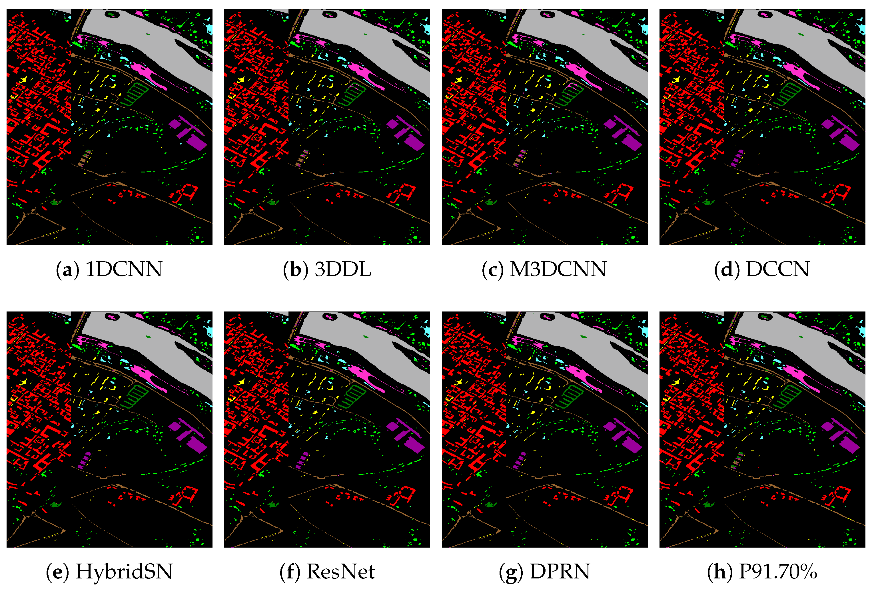
9	90.18	87.67	86.90	98.39	93.53	92.59	99.01	90.63

compares the classification results of the pruned network with the results of other neural network methods. Figure 19 shows the classification maps of different methods on Pavia Center. In the collaborative pruning task in the University of Pavia and Pavia Center datasets, a sparser network structure is obtained on the Pavia Center. OA is still maintained at 97.45%. On the University of Pavia dataset, a 97.39% OA is obtained in Pavia Center, which is better than the original network 3DDL, as well as the results on 1DCNN and M3DCNN. This also proves that proposed method can be applied to larger HSIs.

5. Conclusions

Classification and network pruning tasks for several HSIs are established. In the evolutionary pruning search within each task, important local structural information is acquired and learned. Knowledge transfer between tasks is used to transfer important structures for representation in other tasks to the current task, which guides the learning and optimization of the network on limited labeled samples. It effectively improves the problem of network model overfitting and difficult training caused by limited labeled samples in each task. The self-adaptive transfer strategy based on historical information and dormancy mechanism achieves the original design goal: transferring as much good knowledge as possible and avoiding as much negative knowledge as possible.

Experiments on HSIs show that the proposed method can simultaneously realize classification and structure sparsification on multiple images. By comparing with other pruning methods on image classification data, the proposed method can search for sparser networks while maintaining accuracy. For structured pruning, which is currently more popular, the computation of sparse weight matrices can be avoided, so our future work will consider applying the proposed framework to structured pruning. Therefore, it is necessary to consider knowledge and knowledge transfer strategy in structured pruning. This will further expand our work in the area of neural network architecture optimization. Finally, the proposed method needs to be tested on hardware devices to verify the feasibility and practicability of the method.

References

1. LeCun, Y.; Bengio, Y.; Hinton, G. Deep learning. Nature 2015, 521, 436–444. [Google Scholar] [CrossRef] [PubMed]
2. Ding, Y.; Zhao, X.; Zhang, Z.; Cai, W.; Yang, N.; Zhan, Y. Semi-supervised locality preserving dense graph neural network with ARMA filters and context-aware learning for hyperspectral image classification. IEEE Trans. Geosci. Remote Sens. 2021, 60, 1–12. [Google Scholar] [CrossRef]
3. Ding, Y.; Zhang, Z.; Zhao, X.; Cai, W.; Yang, N.; Hu, H.; Huang, X.; Cao, Y.; Cai, W. Unsupervised self-correlated learning smoothy enhanced locality preserving graph convolution embedding clustering for hyperspectral images. IEEE Trans. Geosci. Remote Sens. 2022, 60, 5536716. [Google Scholar] [CrossRef]
4. Ding, Y.; Zhang, Z.; Zhao, X.; Cai, Y.; Li, S.; Deng, B.; Cai, W. Self-supervised locality preserving low-pass graph convolutional embedding for large-scale hyperspectral image clustering. IEEE Trans. Geosci. Remote Sens. 2022, 60, 5536016. [Google Scholar] [CrossRef]
5. Zhang, M.; Li, W.; Du, Q. Diverse region-based CNN for hyperspectral image classification. IEEE Trans. Image Process. 2018, 27, 2623–2634. [Google Scholar] [CrossRef]
6. Krizhevsky, A.; Sutskever, I.; Hinton, G.E. ImageNet classification with deep convolutional neural networks. Commun. ACM 2017, 60, 84–90. [Google Scholar] [CrossRef] [Green Version]
7. Simonyan, K.; Zisserman, A. Very Deep Convolutional Networks for Large-Scale Image Recognition. In Proceedings of the ICLR 2015: International Conference on Learning Representations 2015, San Diego, CA, USA, 7–9 May 2015. [Google Scholar]
8. Wang, H.; Wu, Z.; Liu, Z.; Cai, H.; Zhu, L.; Gan, C.; Han, S. HAT: Hardware-Aware Transformers for Efficient Natural Language Processing. In Proceedings of the 58th Annual Meeting of the Association for Computational Linguistics, Online, 5–10 July 2020; pp. 7675–7688. [Google Scholar]
9. Liu, Z.; Sun, M.; Zhou, T.; Huang, G.; Darrell, T. Rethinking the Value of Network Pruning. In Proceedings of the International Conference on Learning Representations, Vancouver, BC, Canada, 30 April–3 May 2018. [Google Scholar]
10. LeCun, Y.; Denker, J.S.; Solla, S.A. Optimal Brain Damage. Adv. Neural Inf. Process. Syst. 1989, 2, 598–605. [Google Scholar]
11. Han, S.; Pool, J.; Tran, J.; Dally, W.J. Learning Both Weights and Connections for Efficient Neural Networks. In Proceedings of the 28th International Conference on Neural Information Processing Systems, NIPS’15, Montreal, QC, Canada, 7–12 December 2015; MIT Press: Cambridge, MA, USA, 2015; Volume 1, pp. 1135–1143. [Google Scholar]
12. Lee, J.; Park, S.; Mo, S.; Ahn, S.; Shin, J. Layer-adaptive sparsity for the magnitude-based pruning. arXiv 2020, arXiv:2010.07611. [Google Scholar]
13. Wang, Y.; Li, D.; Sun, R. NTK-SAP: Improving neural network pruning by aligning training dynamics. arXiv 2023, arXiv:2304.02840. [Google Scholar]
14. Qi, B.; Chen, H.; Zhuang, Y.; Liu, S.; Chen, L. A Network Pruning Method for Remote Sensing Image Scene Classification. In Proceedings of the 2019 IEEE International Conference on Signal, Information and Data Processing (ICSIDP), Chongqing, China, 11–13 December 2019; pp. 1–4. [Google Scholar]
15. Wang, Z.; Xue, W.; Chen, K.; Ma, S. Remote Sensing Image Classification Based on Lightweight Network and Pruning. In Proceedings of the 2022 China Automation Congress (CAC), Xiamen, China, 25–27 November 2022; pp. 3186–3191. [Google Scholar]
16. Guo, X.; Hou, B.; Ren, B.; Ren, Z.; Jiao, L. Network pruning for remote sensing images classification based on interpretable CNNs. IEEE Trans. Geosci. Remote Sens. 2021, 60, 1–15. [Google Scholar] [CrossRef]
17. Jung, I.; You, K.; Noh, H.; Cho, M.; Han, B. Real-time object tracking via meta-learning: Efficient model adaptation and one-shot channel pruning. In Proceedings of the AAAI Conference on Artificial Intelligence, New York, NY, USA, 7–12 February 2020; Volume 34, pp. 11205–11212. [Google Scholar]
18. He, Y.; Lin, J.; Liu, Z.; Wang, H.; Li, L.J.; Han, S. Amc: Automl for model compression and acceleration on mobile devices. In Proceedings of the European conference on computer vision (ECCV), Munich, Germany, 8–14 September 2018; pp. 784–800. [Google Scholar]
19. Zhou, Y.; Yen, G.G.; Yi, Z. Evolutionary compression of deep neural networks for biomedical image segmentation. IEEE Trans. Neural Netw. Learn. Syst. 2019, 31, 2916–2929. [Google Scholar] [CrossRef]
20. Wu, T.; Li, X.; Zhou, D.; Li, N.; Shi, J. Differential Evolution Based Layer-Wise Weight Pruning for Compressing Deep Neural Networks. Sensors 2021, 21, 880. [Google Scholar] [CrossRef]
21. Wu, T.; Shi, J.; Zhou, D.; Lei, Y.; Gong, M. A Multi-objective Particle Swarm Optimization for Neural Networks Pruning. In Proceedings of the 2019 IEEE Congress on Evolutionary Computation (CEC), Wellington, New Zealand, 10–13 June 2019; pp. 570–577. [Google Scholar]
22. Zhou, Y.; Yen, G.G.; Yi, Z. A Knee-Guided Evolutionary Algorithm for Compressing Deep Neural Networks. IEEE Trans. Syst. Man Cybern. 2021, 51, 1626–1638. [Google Scholar] [CrossRef]
23. Zhao, J.; Yang, C.; Zhou, Y.; Zhou, Y.; Jiang, Z.; Chen, Y. Multi-Objective Net Architecture Pruning for Remote Sensing Classification. In Proceedings of the 2021 IEEE International Geoscience and Remote Sensing Symposium IGARSS, Brussels, Belgium, 11–16 July 2021; pp. 4940–4943. [Google Scholar]
24. Wei, X.; Zhang, N.; Liu, W.; Chen, H. NAS-Based CNN Channel Pruning for Remote Sensing Scene Classification. IEEE Geosci. Remote Sens. Lett. 2022, 19, 1–5. [Google Scholar] [CrossRef]
25. Ma, X.; Zhao, L.; Huang, G.; Wang, Z.; Hu, Z.; Zhu, X.; Gai, K. Entire space multi-task model: An effective approach for estimating post-click conversion rate. In Proceedings of the 41st International ACM SIGIR Conference on Research & Development in Information Retrieval, Ann Arbor, MI, USA, 8–12 July 2018; pp. 1137–1140. [Google Scholar]
26. Ruder, S. An overview of multi-task learning in deep neural networks. arXiv 2017, arXiv:1706.05098. [Google Scholar]
27. Hou, Y.; Jiang, N.; Ge, H.; Zhang, Q.; Qu, X.; Feng, L.; Gupta, A. Memetic Multi-agent Optimization in High Dimensions using Random Embeddings. In Proceedings of the 2019 IEEE Congress on Evolutionary Computation (CEC), Wellington, New Zealand, 10–13 June 2019; pp. 135–141. [Google Scholar] [CrossRef]
28. Shi, J.; Zhang, X.; Tan, C.; Lei, Y.; Li, N.; Zhou, D. Multiple datasets collaborative analysis for hyperspectral band selection. IEEE Geosci. Remote Sens. Lett. 2021, 19, 1–5. [Google Scholar] [CrossRef]
29. Liu, S.; Shi, Q. Multitask deep learning with spectral knowledge for hyperspectral image classification. IEEE Geosci. Remote Sens. Lett. 2020, 17, 2110–2114. [Google Scholar] [CrossRef] [Green Version]
30. Zhang, L.; Zhang, L.; Du, B. Deep learning for remote sensing data: A technical tutorial on the state of the art. IEEE Geosci. Remote Sens. Mag. 2016, 4, 22–40. [Google Scholar] [CrossRef]
31. Chen, Y.; Lin, Z.; Zhao, X.; Wang, G.; Gu, Y. Deep learning-based classification of hyperspectral data. IEEE J. Sel. Top. Appl. Earth Obs. Remote Sens. 2014, 7, 2094–2107. [Google Scholar] [CrossRef]
32. Mou, L.; Ghamisi, P.; Zhu, X.X. Deep recurrent neural networks for hyperspectral image classification. IEEE Trans. Geosci. Remote Sens. 2017, 55, 3639–3655. [Google Scholar] [CrossRef] [Green Version]
33. Ding, Y.; Zhang, Z.; Zhao, X.; Hong, D.; Cai, W.; Yang, N.; Wang, B. Multi-scale receptive fields: Graph attention neural network for hyperspectral image classification. Expert Syst. Appl. 2023, 223, 119858. [Google Scholar] [CrossRef]
34. Ding, Y.; Zhang, Z.; Zhao, X.; Hong, D.; Cai, W.; Yu, C.; Yang, N.; Cai, W. Multi-feature fusion: Graph neural network and CNN combining for hyperspectral image classification. Neurocomputing 2022, 501, 246–257. [Google Scholar] [CrossRef]
35. Zhang, Z.; Ding, Y.; Zhao, X.; Siye, L.; Yang, N.; Cai, Y.; Zhan, Y. Multireceptive field: An adaptive path aggregation graph neural framework for hyperspectral image classification. Expert Syst. Appl. 2023, 217, 119508. [Google Scholar] [CrossRef]
36. Hamida, A.B.; Benoit, A.; Lambert, P.; Amar, C.B. 3-D deep learning approach for remote sensing image classification. IEEE Trans. Geosci. Remote Sens. 2018, 56, 4420–4434. [Google Scholar] [CrossRef] [Green Version]
37. Li, H.C.; Lin, Z.X.; Ma, T.Y.; Zhao, X.L.; Plaza, A.; Emery, W.J. Hybrid Fully Connected Tensorized Compression Network for Hyperspectral Image Classification. IEEE Trans. Geosci. Remote Sens. 2023, 61, 1–16. [Google Scholar] [CrossRef]
38. Ahmad, M.; Khan, A.M.; Mazzara, M.; Distefano, S.; Ali, M.; Sarfraz, M.S. A fast and compact 3-D CNN for hyperspectral image classification. IEEE Geosci. Remote Sens. Lett. 2020, 19, 1–5. [Google Scholar] [CrossRef]
39. Cao, X.; Ren, M.; Zhao, J.; Li, H.; Jiao, L. Hyperspectral imagery classification based on compressed convolutional neural network. IEEE Geosci. Remote Sens. Lett. 2019, 17, 1583–1587. [Google Scholar] [CrossRef]
40. Verma, V.K.; Singh, P.; Namboodri, V.; Rai, P. A“Network Pruning Network”Approach to Deep Model Compression. In Proceedings of the IEEE/CVF Winter Conference on Applications of Computer Vision, Snowmass Village, CO, USA, 1–5 March 2020; pp. 3009–3018. [Google Scholar]
41. Castellano, G.; Fanelli, A.M.; Pelillo, M. An iterative pruning algorithm for feedforward neural networks. IEEE Trans. Neural Netw. 1997, 8, 519–531. [Google Scholar] [CrossRef]
42. Li, H.; Kadav, A.; Durdanovic, I.; Samet, H.; Graf, H.P. Pruning filters for efficient convnets. arXiv 2016, arXiv:1608.08710. [Google Scholar]
43. Zhang, S.; Stadie, B.C. One-Shot Pruning of Recurrent Neural Networks by Jacobian Spectrum Evaluation. In Proceedings of the ICLR 2020: Eighth International Conference on Learning Representations, Addis Ababa, Ethiopia, 26–30 April 2020. [Google Scholar]
44. Chen, T.; Ji, B.; Ding, T.; Fang, B.; Wang, G.; Zhu, Z.; Liang, L.; Shi, Y.; Yi, S.; Tu, X. Only train once: A one-shot neural network training and pruning framework. Adv. Neural Inf. Process. Syst. 2021, 34, 19637–19651. [Google Scholar]
45. Gupta, A.; Ong, Y.S.; Feng, L. Multifactorial Evolution: Toward Evolutionary Multitasking. IEEE Trans. Evol. Comput. 2016, 20, 343–357. [Google Scholar] [CrossRef]
46. Gupta, A.; Ong, Y.S.; Feng, L.; Tan, K.C. Multiobjective Multifactorial Optimization in Evolutionary Multitasking. IEEE Trans. Syst. Man Cybern. 2017, 47, 1652–1665. [Google Scholar] [CrossRef]
47. Tan, K.C.; Feng, L.; Jiang, M. Evolutionary transfer optimization-a new frontier in evolutionary computation research. IEEE Comput. Intell. Mag. 2021, 16, 22–33. [Google Scholar] [CrossRef]
48. Thang, T.B.; Dao, T.C.; Long, N.H.; Binh, H.T.T. Parameter adaptation in multifactorial evolutionary algorithm for many-task optimization. Memetic Comput. 2021, 13, 433–446. [Google Scholar] [CrossRef]
49. Shen, F.; Liu, J.; Wu, K. Evolutionary multitasking network reconstruction from time series with online parameter estimation. Knowl.-Based Syst. 2021, 222, 107019. [Google Scholar] [CrossRef]
50. Tang, Z.; Gong, M.; Xie, Y.; Li, H.; Qin, A.K. Multi-task particle swarm optimization with dynamic neighbor and level-based inter-task learning. IEEE Trans. Emerg. Top. Comput. Intell. 2021, 6, 300–314. [Google Scholar] [CrossRef]
51. Li, H.; Ong, Y.S.; Gong, M.; Wang, Z. Evolutionary Multitasking Sparse Reconstruction: Framework and Case Study. IEEE Trans. Evol. Comput. 2019, 23, 733–747. [Google Scholar] [CrossRef]
52. Chandra, R.; Gupta, A.; Ong, Y.S.; Goh, C.K. Evolutionary Multi-task Learning for Modular Training of Feedforward Neural Networks. In Proceedings of the 23rd International Conference on Neural Information Processing, Kyoto, Japan, 16–21 October 2016; Volume 9948, pp. 37–46. [Google Scholar]
53. Chandra, R.; Gupta, A.; Ong, Y.S.; Goh, C.K. Evolutionary Multi-task Learning for Modular Knowledge Representation in Neural Networks. Neural Process. Lett. 2018, 47, 993–1009. [Google Scholar] [CrossRef]
54. Chandra, R. Co-evolutionary Multi-task Learning for Modular Pattern Classification. In Proceedings of the International Conference on Neural Information Processing, Guangzhou, China, 14–18 November 2017; pp. 692–701. [Google Scholar]
55. Tang, Z.; Gong, M.; Zhang, M. Evolutionary multi-task learning for modular extremal learning machine. In Proceedings of the 2017 IEEE Congress on Evolutionary Computation (CEC), Donostia, Spain, 5–8 June 2017. [Google Scholar]
56. Gao, W.; Cheng, J.; Gong, M.; Li, H.; Xie, J. Multiobjective Multitasking Optimization With Subspace Distribution Alignment and Decision Variable Transfer. IEEE Trans. Emerg. Top. Comput. Intell. 2021, 6, 818–827. [Google Scholar] [CrossRef]
57. Deb, K.; Goyal, M. A combined genetic adaptive search (GeneAS) for engineering design. Comput. Sci. Inform. 1996, 26, 30–45. [Google Scholar]
58. Caruana, R. Multitask learning. Mach. Learn. 1997, 28, 41–75. [Google Scholar] [CrossRef]
59. Frankle, J.; Carbin, M. The lottery ticket hypothesis: Finding sparse, trainable neural networks. arXiv 2018, arXiv:1803.03635. [Google Scholar]
60. Green, R.O.; Eastwood, M.L.; Sarture, C.M.; Chrien, T.G.; Aronsson, M.; Chippendale, B.J.; Faust, J.A.; Pavri, B.E.; Chovit, C.J.; Solis, M.; et al. Imaging spectroscopy and the airborne visible/infrared imaging spectrometer (AVIRIS). Remote Sens. Environ. 1998, 65, 227–248. [Google Scholar] [CrossRef]
61. Li, Y.; Zhang, H.; Shen, Q. Spectral–spatial classification of hyperspectral imagery with 3D convolutional neural network. Remote Sens. 2017, 9, 67. [Google Scholar] [CrossRef] [Green Version]
62. He, M.; Li, B.; Chen, H. Multi-scale 3D deep convolutional neural network for hyperspectral image classification. In Proceedings of the 2017 IEEE International Conference on Image Processing (ICIP), Beijing, China, 17–20 September 2017; pp. 3904–3908. [Google Scholar]
63. Hu, W.; Huang, Y.; Wei, L.; Zhang, F.; Li, H. Deep convolutional neural networks for hyperspectral image classification. J. Sens. 2015, 2015, 258619. [Google Scholar] [CrossRef] [Green Version]
64. Yu, H.; Zhang, H.; Liu, Y.; Zheng, K.; Xu, Z.; Xiao, C. Dual-channel convolution network with image-based global learning framework for hyperspectral image classification. IEEE Geosci. Remote Sens. Lett. 2021, 19, 1–5. [Google Scholar] [CrossRef]
65. Roy, S.K.; Krishna, G.; Dubey, S.R.; Chaudhuri, B.B. HybridSN: Exploring 3-D–2-D CNN feature hierarchy for hyperspectral image classification. IEEE Geosci. Remote Sens. Lett. 2019, 17, 277–281. [Google Scholar] [CrossRef] [Green Version]
66. Roy, S.K.; Manna, S.; Song, T.; Bruzzone, L. Attention-based adaptive spectral–spatial kernel ResNet for hyperspectral image classification. IEEE Trans. Geosci. Remote Sens. 2020, 59, 7831–7843. [Google Scholar] [CrossRef]
67. Paoletti, M.E.; Haut, J.M.; Fernandez-Beltran, R.; Plaza, J.; Plaza, A.J.; Pla, F. Deep pyramidal residual networks for spectral–spatial hyperspectral image classification. IEEE Trans. Geosci. Remote Sens. 2018, 57, 740–754. [Google Scholar] [CrossRef]
68. Han, S.; Mao, H.; Dally, W.J. Deep Compression: Compressing Deep Neural Networks with Pruning, Trained Quantization and Huffman Coding. In Proceedings of the ICLR 2016: International Conference on Learning Representations 2016, San Juan, Puerto Rico, 2–4 May 2016. [Google Scholar]
69. Yang, Z.; Xi, Z.; Zhang, T.; Guo, W.; Zhang, Z.; Li, H.C. CMR-CNN: Cross-mixing residual network for hyperspectral image classification. IEEE J. Sel. Top. Appl. Earth Obs. Remote Sens. 2022, 15, 8974–8989. [Google Scholar] [CrossRef]
70. Srinivas, S.; Babu, R.V. Data-free parameter pruning for deep neural networks. arXiv 2015, arXiv:1507.06149. [Google Scholar]
Figure 1. Spectral curves of Indian Pines and Salinas under AVIRIS.
Remotesensing 15 03084 g001
Figure 2. HSI classification based on neural networks.
Remotesensing 15 03084 g002
Figure 3. The procedure of neural network pruning.
Remotesensing 15 03084 g003
Figure 4. The overview of evolutionary multi-task optimization.
Remotesensing 15 03084 g004
Figure 5. Overall framework of proposed network collaborative pruning method for HSI classification.
Remotesensing 15 03084 g005
Figure 6. The proposed evolutionary multi-task pruning algorithm.
Remotesensing 15 03084 g006
Figure 7. The representation of individual initialization.
Remotesensing 15 03084 g007
Figure 8. The illustration of crossover operator.
Remotesensing 15 03084 g008
Figure 9. Illustration of mutation operator.
Remotesensing 15 03084 g009
Figure 10. The false-color image and reference image on Indian Pines dataset.
Remotesensing 15 03084 g010
Figure 11. The false-color image and reference image on Salinas dataset.
Remotesensing 15 03084 g011
Figure 12. The false-color image and reference image on University of Pavia dataset.
Remotesensing 15 03084 g012
Figure 13. Classification maps on Indian Pines, Salinas and University of Pavia. Where P represents Pruned Network.
Remotesensing 15 03084 g013
Figure 14. The Pareto-optimal front without fine-tuning after completing evolutionary search on two groups experiments.
Remotesensing 15 03084 g014
Figure 15. Hypervolume curves of the evolutionary process on two groups experiments.
Remotesensing 15 03084 g015
Figure 16. Classification maps on Indian Pines, Salinas, and University of Pavia datasets. GT represents ground truth and P represents pruned network.
Remotesensing 15 03084 g016aRemotesensing 15 03084 g016b
Figure 17. Knowledge transfer between tasks: the left column uses the Indian Pines dataset as another task of collaborative pruning, and the right column uses the University of Pavia datatset as another task of collaborative pruning.
Remotesensing 15 03084 g017
Figure 18. The false-color image and reference image on Pavia Center dataset.
Remotesensing 15 03084 g018
Figure 19. Classification maps on Pavia Center. Where P represents Pruned Network.
Remotesensing 15 03084 g019