Deep Convolutional Neural Network for Plume Rise Measurements in Industrial Environments

Abstract

Determining the height of plume clouds is crucial for various applications, including global climate models. Smokestack plume rise refers to the altitude at which the plume cloud travels downwind until its momentum dissipates and the temperatures of the plume cloud and its surroundings become equal. While most air-quality models employ different parameterizations to forecast plume rise, they have not been effective in accurately estimating it. This paper introduces a novel framework that utilizes Deep Convolutional Neural Networks (DCNNs) to monitor smokestack plume clouds and make real-time, long-term measurements of plume rise. The framework comprises three stages. In the first stage, the plume cloud is identified using an enhanced Mask R-CNN, known as the Deep Plume Rise Network (DPRNet). Next, image processing analysis and least squares theory are applied to determine the plume cloud’s boundaries and fit an asymptotic model to its centerlines. The z-coordinate of the critical point of this model represents the plume rise. Finally, a geometric transformation phase converts image measurements into real-world values. This study’s findings indicate that the DPRNet outperforms conventional smoke border detection and recognition networks. In quantitative terms, the proposed approach yielded a 22% enhancement in the F1 score, compared to its closest competitor, DeepLabv3.

1. Introduction

The Smokestack Plume Cloud (PC) rises due to two main factors, momentum and buoyancy. Momentum refers to the force the pollutants generate as they are expelled upward from the smokestack, and this force propels the PC upward and helps to counteract the downward pull of gravity. Buoyancy is caused by the higher temperature of the plume effluent, which results in a lower density of the PC relative to the surrounding air. When the PC dissipates and mixes with the surrounding air, it becomes neutrally buoyant and loses its vertical momentum. It is then carried downwind at a constant height called the Plume Rise (PR) or plume rise height. Predicting the PR is a significant challenge in estimating the dispersion of harmful effluents in the air [1]. Accurate PR measurement is crucial for various research and operational applications, such as air-quality transport models, local environment assessment cases, and global climate models [2]. PR contributes to (1) the distance pollutants are carried downwind, (2) their concentration at the surface where they are deposited in the environment or inhaled by people, and (3) the amounts of greenhouse gases mixed into the upper troposphere.

Briggs developed the parameterizations of PR prediction in the 1960s using dimensional analysis to estimate the PR based on smokestack parameters and meteorological measurements in various atmospheric conditions [3,4]. Early observations of PR were used to test and rectify the parameterizations developed using dimensional analysis [5]. Several calibration techniques were employed, including wind tunnel studies and field observations utilizing film photography, theodolites, and cloud-height searchlights [6]. Additionally, there are 3D air-quality models that utilize parameterization equations, such as GEM-MACH [7], CAMx [8], and CMAQ [9].

Several studies in the 1970s and 1980s tested the parameterizations of PR prediction by comparing them to actual observations, demonstrating that the Briggs equations tend to overestimate the PR [10,11,12,13]. In 1993, an aircraft-based measurement was conducted to measure ${\mathrm{SO}}_2$ emissions from a power plant, indicating an overestimation of about 400 m in the PR [14]. However, in 2002, Webster et al. [15] performed surface measurements and concluded that the Briggs parameterizations tend to underestimate PR. In 2013, an aerial measurement study was conducted as part of the Canada–Alberta Joint Oil Sands Monitoring (JOSM) Plan in the Athabasca oil sands region of northern Alberta [16,17,18]. The project consisted of 84 flight hours of an instrumented Convair aircraft over 21 flights designed to measure pollutant emissions, study the transformation of chemicals downwind of the industry, and verify satellite measurements of pollutants and greenhouse gases in the region. Using aircraft-based measurements and reported smokestack parameters and meteorological data, it was demonstrated that the Briggs equations significantly underestimate PR at this location.

Due to the need for further testing and possible modification of the Briggs equations based on modern observation techniques, recent advancements in environmental monitoring activities have been made to improve safety and pollution prevention in industrial regions [19,20,21,22]. Additionally, several smoke border detection and recognition models have been introduced recently using digital image analysis, such as wavelet and support vector machines [23], LBP and LBPV pyramids [24], multi-scale partitions with AdaBoost [25], and high-order local ternary patterns [26], which have proven to be well-performed and impressive. These advancements have led to the development of instrumentation that can be deployed near any smokestack to provide information on pollutant dispersion and potential exposure to people downwind. This information is based on actual real-time observation, i.e., digital images, as opposed to potentially erroneous and decades-old parameterizations. Since there is a lack of research on PC recognition, smoke recognition studies will be reviewed in the following, given the similarity of our work to smoke recognition.

To find the smoke within an image or a video frame, either a rough location of smoke is identified using bounding boxes called smoke border detection [27], or pixels are identified and classified in detail, named smoke recognition [28]. Due to the translucent edges of smoke clouds, the recognition task needs far more accuracy than border detection. Traditional smoke recognition methods utilize manual features, which lead to low-accuracy recognition results due to a large variety of smoke appearances. These low-level features consist of motion characteristic analysis of the smoke [29], smoke colour [30], and smoke shape [31]. In another research, ref. [32] took advantage of the Gaussian Mixture Model (GMM) to detect the motion region of the smoke and [33] combined rough set and region growing methods as a smoke recognition algorithm which seems to be a time-consuming algorithm due to the computational burden of the region growing process. Since using colour information is less effective due to the similarity of smoke colour to its surrounding environment, the combination of motion and colour characteristics is considered for smoke recognition [34]. Some algorithms utilize infrared images and video frames in their experiments [35], which are not easily accessible and can increase the project’s costs. Moreover, using digital images makes the algorithm more flexible as it can be used with more hardware. On the other hand, some smokes are too close to the background temperature to be captured by the near red-channel wavelength. A higher-order dynamical system introduced in 2017 used particle swarm optimization for smoke pattern analysis [36]. However, this approach had a low border detection rate and high computational complexity.

In recent years, deep learning-based methods, especially Convolutional Neural Network (CNN)-based methods, have led to significant results in semantic segmentation [37] and object recognition [38]. Similarly, these methods are widely used in smoke border detection and recognition [39,40,41] with different architectures, such as three-layer CNN [42], generative adversarial network (GAN) [43], and two-path Fully Convolutional Network (FCN) [44]. Recently, a count prior embedding method was proposed for smoke recognition to extract information about the counts of different pixels (smoke and non-smoke) [45]. Experimental results showed an improvement in the recognition performance of these studies. However, the high computational complexities of these huge models are an obstacle to their use in PR real-time observations.

We have proposed a novel framework using Deep Convolutional Neural Network (DCNN) algorithms to measure PR. Our approach comprises three stages, (1) recognizing the PC region using an improved Mask R-CNN, (2) extracting the PC’s Neutral Buoyancy Point (NBP) from the centerline of the recognized PC, and (3) transforming the PC’s geometric measurement from an image-scale to real-world scale. Figure 1 illustrates the framework of obtaining PR information using DCNN.

This strategy accurately recognizes the PC and measures PR in real-time. Here, we reinforce the bounding box loss function in Region Proposal Network (RPN) [46,47] through engaging a new regularization to the loss function. This regularizer restricts the search domain of RPN to the smokestack exit. In other words, it minimizes the distance between the proposed bounding boxes and the desired smokestack exit, called smokestack exit loss ($L_S$). The proposed method is also computationally economical because it generates only a limited number of anchor boxes swarmed across the desired smokestack exit. Consequently, the main contributions of this paper can be summarized as follows:

• Proposing Deep Plume Rise Network (DPRNet), a deep learning method for PR measurements, by incorporating PC recognition and image processing-based measurements. We have provided a reproducible algorithm to recognize PCs from RGB images accurately.
• To the best of our knowledge, this paper estimates the PCs’ neutral buoyancy coordinates for the first time, which is of the essence in environmental studies. This online information can help update related criteria, such as the live air-quality health index (AQHI).
• A pixel-level recognition dataset, Deep Plume Rise Dataset (DPRD), containing (1) 2500 fine segments of PCs, (2) the upper and lower boundaries of PCs, (3) the image coordinates of smokestack exit, (4) the centerlines and NBP image coordinates of PCs, is presented. As is expected, the DPRD dataset includes one class, namely PC. Widely-used DCNN-based smoke recognition methods are employed to evaluate our dataset. Furthermore, this newly generated dataset was used for PR measurements.

This paper is organized as follows—Section 2 briefly explains the theoretical information used in our proposed framework. Section 3 describes our proposed framework for measuring the PR of a desired smokestack. Then, Section 4 presents our dataset collection procedure, under-study site, experimental results of the proposed method and evaluation results using different metrics, and PR and PR distance calculations. Finally, this research’s conclusions, findings, and future studies are expressed in Section 5.

2. Theoretical Background

2.1. Briggs PR Prediction

The plume rise (PR) computation presents a challenging problem in anticipating the dispersion of detrimental pollutants in atmospheric science [1]. PR is influenced by two factors, buoyancy and momentum. Generally, PCs exhibit buoyancy, indicating that they possess a higher temperature than the surrounding air. This causes them to ascend due to their lower density than the ambient air. Additionally, PCs exhibit vertical velocity and momentum upon exiting the smokestack, resulting in further elevation. However, PCs may also descend under the influence of gravity when they are cold and dense, or when nearby obstructions force them to travel downwind [48]. In 1975, Briggs introduced a formula for estimating the maximum PR distance, which proved to be practically useful in PR calculations [4].

It is important to mention that when assessing the wind speed at the local PC height rather than the source height, iterative calculations are required [49,50]. The wind has a considerable impact on PC buoyancy, horizontal momentum movements, and PR [1]. Furthermore, PR remains unaltered by wind speed fluctuations under stable conditions with low turbulence, which complicates the measurement process. Nevertheless, substantial PR variations have been observed in unstable conditions at a constant downwind distance.

2.2. CNN and Convolutional Layer

Convolutional Neural Networks (CNNs) are specialized types of neural networks designed for handling grid data, such as image data arranged in a two-dimensional or three-dimensional pixel mesh structure. The term “CNN” originates from the inclusion of convolutional layers within the network. Each convolutional layer consists of multiple kernels and biases that are applied locally to the input, generating a feature map or activation map according to the number of filters. Assuming the convolutional layer is implemented in a two-dimensional fashion on the input image, the $j^{th}$ feature map $O_j$, derived from the $j^{th}$ kernel, is computed at the position $(x,y)$ as [51],

$$O_j^{xy}=B_j+\sum _k\sum _{m=0}^{M-1}\sum _{n=0}^{N-1}{w}_j^{mn}{z}_k^{(x+m)(y+n)}$$

(1)

where k moves along the depth dimension of input $z\in {\mathbb{R}}^{p\times q\times r}$ and $w_j^{mn}$ is the two-dimensional kernel weight $W\in {\mathbb{R}}^{M\times N}$ at position $(m,n)$. $B_j$ is the bias matrix.

2.3. Mask R-CNN

Mask R-CNN, a member of the region-based CNN family, was proposed in [52] and has been widely employed for various identification tasks, including recognition within the COCO dataset. Initially, RCNN was presented in [53], where computer vision techniques were utilized to generate region proposals. Subsequently, Fast RCNN was introduced in [47], incorporating a CNN before region proposals to decrease execution time. In 2017, Faster RCNN continued this progression by introducing the Region Proposal Network (RPN) to propose regions of interest (ROIs) [54]. Ultimately, Mask R-CNN, an extension of Faster RCNN, integrated an additional CNN for pixel-level recognition of detected object boundaries. Mask R-CNN is a relatively straightforward model and is easily adaptable to similar tasks [52]. As a result, Mask R-CNN can generate pixel-level masks for objects in addition to performing object localization and classification tasks.

2.3.1. RPN

A Region Proposal Network (RPN) is a deep Fully Convolutional Network (FCN) that suggests regions and plays a critical role in Mask R-CNN. RPN assists in selectively concentrating on valuable aspects within input images. This network takes an image as input and outputs a set of region proposals alongside their objectness scores. It slides a window over the convolutional feature map (backbone output) and maps it to a lower-dimensional feature. This generated feature is then fed into two fully-connected layers to determine the proposed regions class (object vs. non-object) and the four corresponding coordinates [54]. For each sliding window location, a maximum of k potential proposals are parameterized relative to k reference boxes or anchors. RPN is trained end-to-end using back-propagation and stochastic gradient descent. Figure 2 illustrates an RPN scheme, where the proposed regions are produced as module outputs.

2.3.2. Loss Function

Mask R-CNN loss function is a weighted summation of other losses related to different sections of this comprehensive model. As a definition based on [52], a multi-task loss function is proposed on each sampled ROI as,

$$L=L_{cls}+L_{reg}+L_{msk}$$

(2)

where $L_{cls}$ recognizes the class type of each object while $L_{reg}$ attempts to find the optimum anchor box for each object. Note that, in this study, we have one class, PC. $L_{msk}$ tries to recognize the optimum object’s segment in each bounding box.

3. Methodology

The proposed framework for PR measurement is depicted in Figure 3. Images containing PC(s) are input to the DPRNet for PC boundary detection and recognition. PR and PR distance are subsequently measured based on the extraction of the NBP from DPRNet’s output. The image coordinates of the NBP are combined with wind direction data for processing through geometric transformation calculations. The primary output of the system provides the PR as a physical height and the PR distance downwind at which the PR occurs. Additionally, a schematic diagram in Figure 4 illustrates the definitions of the PC centerline, PR, and PR distance.

3.1. DPRNet

The objective of this research is to accurately identify the PC of the target smokestack from a broad range of image datasets captured within the study area. DPRNet is a customized version of Mask R-CNN, featuring two innovative smokestack PR measurement modules, (1) the physical module and (2) the loss regularizer module. These modules enhance the Region Proposal Network’s (RPN) performance in pinpointing the most probable proposal PCs. Mask R-CNN, the foundation of the proposed method, is a widely used boundary detection and recognition technique. This robust framework accounts for the irregular shapes of PCs, their translucent edges, and similar pixel values compared to their background [52]. As illustrated in Figure 5, DPRNet is an application-oriented adaptation of Mask R-CNN, augmented with two novel modules.

In this architecture, ResNet50 [55] serves as the backbone network for extracting feature maps from input images. The Feature Pyramid Network (FPN) utilizes these feature maps to produce multi-scale feature maps, which contain more valuable information than conventional feature pyramids. Subsequently, the Region Proposal Network (RPN) identifies the PC by sliding a window over these feature maps, predicting the presence of a PC and locating it through the creation of bounding boxes. Consequently, a set of PC proposals from RPN and the feature map generated by the backbone network are obtained. The ROI Align module scales the proposals to the feature map level and prevents misalignment by standardizing the proposals’ aspect ratios. Finally, these refined feature maps are directed to three distinct outputs. The first output is a classification block that determines whether the ROI corresponds to the foreground (PC). The second output is a regression block that predicts bounding boxes based on the provided ground truth. The last output is a recognition mask for the detected PC, generated using a Fully Convolutional Network (FCN) [56].

Two modules are incorporated into Mask R-CNN to enhance its effectiveness and decrease computational complexity. The first module, a basic image processing module, estimates the smokestack. The second module aims to improve the loss associated with $L_{reg}$ by introducing a regularizer loss, detailed in Section 3.1.2. These modules are thoroughly discussed in the subsequent subsections.

3.1.1. Physical Module

The physical module is designed to identify an exit point from which the PC of interest emerges from a chimney stack situated in the center of the image. It is important to note that this module is utilized only during the training phase, while the exit point is automatically predicted during the network’s inference process without the physical module. In the physical module, the smokestack exit is detected from the ground truth binary image using an image processing technique that identifies extrema points of foreground boundaries [57]. It is logical that the smokestack exit is the plausible region for the plume rise. Consequently, proposed regions can be considered around this point (Figure 5). This module ensures that the method does not detect small PC fragments occasionally visible in different parts of images apart from the smokestack exit.

To identify the smokestack exit, eight extrema points on each PC’s boundary are extracted based on image processing analysis [57], as depicted in Figure 6. This algorithm first smooths noise in the foreground regions (i.e., the PC region labelled in the ground truth imagery). It then tracks boundary pixels of the foreground region and extracts eight extrema points exhibiting the locally highest geometric curvature. The bottom-left corner of each PC segment is regarded as the smokestack exit point of S in the world coordinate depicted in Figure 4 and Figure 7. Furthermore, the corresponding point in the image coordinate is s, depicted in Figure 8.

3.1.2. Loss Regularizer Module

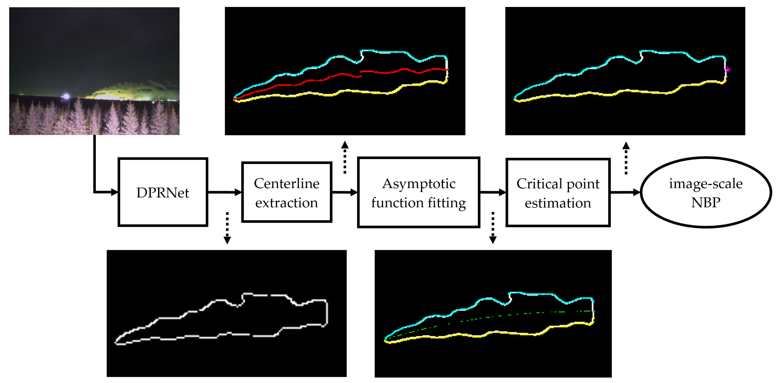
As discussed in Section 2.3.2, defining an effective loss function is crucial for stabilizing the model. In this context, a new regularizer is added to the loss function, which regresses the coordinates of the most plausible PC regions. In fact, the aim is to minimize the distance between the bounding boxes proposed by the RPN and the smokestack exit. Consider a box with coordinates ($x,z,w,h$) defined here. In that case, the regression loss related to the smokestack exit can be defined as,

$$L_S=R(u-u^{*}),$$

(3)

in which,

$$\begin{array}{c}\hfill u_x=\frac{x-x_a}{w_a},u_z=\frac{z-z_a}{h_a},u_w=log\left(\frac{w}{w_a}\right),u_h=log\left(\frac{h}{h_a}\right),\\ \hfill u_x^{*}=\frac{x^{*}-x_a}{w_a},u_z^{*}=\frac{z^{*}-z_a}{h_a},u_w^{*}=log\left(\frac{w^{*}}{w_a}\right),u_h^{*}=log\left(\frac{h^{*}}{h_a}\right)\end{array}$$

(4)

where u and $u^{*}$ represent the coordinates of our predicted and ground truth smokestack exit and R is the robust loss function. Note that the subscript a and superscript ∗ variables denote the anchor coordinate and ground truth coordinates, respectively, while the remaining variables represent the predicted coordinates. The point $(x,z)$ specifies the location of the bounding box’s top-left corner, and the parameters w and h correspond to the width and height of the bounding box, respectively.

In contrast to the Mask R-CNN model, DPRNet’s loss regularizer module ($L_S$) minimizes recognition task errors for a specific PC, addressing the primary issues of this model, such as missing the desired smokestack exit and proposing multiple boxes for a single PC. $L_S$ aids in preventing the need to span the entire image pixels, which leads to high training times and computational complexities.

3.2. NBP Extraction

As illustrated in Figure 3, PR measurements are carried out based on extracting the NBP for each PC image. This point is depicted as p in the image coordinate and P in the real-world coordinates in Figure 7 and Figure 8. The NBP extraction phase can be summarized in three steps, with an overall processing chain shown in Figure 9. In the first step, the PC’s centerline is extracted as a curve representing the meandering of the PC. This is achieved by dividing the boundary pixels of the PC into two categories: upper and lower boundary pixels, displayed as cyan and yellow-coloured lines, respectively, in Figure 9. The upper and lower boundaries are determined by identifying the highest and lowest white pixels in the binary PC image. This method enables the extraction of the PC’s skeletonized curve, the centerline, by calculating the mean of the upper and lower points. This binary classification of boundary lines is performed by tracking the upper pixel at the highest row index, while the lowest one for the lower boundary pixel is determined from each fixed column index with the coordinate origin at the lower-left corner of the image space. The centerline pixel per column is found by simply averaging the two-row indices.

Measuring the NBP for plume rise in the context of atmospheric science using imagery requires identifying the point at which the buoyant force from the plume is equal to the gravitational force acting on it. At this point, the plume stops rising further and begins to spread laterally. The central lines detected from the imagery display prominent visual cues caused by various factors involved in atmospheric dynamics. However, they cannot explicitly estimate the NBP and necessitate a physical interpretation to determine the NBP from the centerlines. Consequently, an asymptotic function [58] is fitted to the centerline pixels using a conventional least-squared method to derive this function’s horizontal asymptote, which helps determine the NBP from the imagery. Equation (5) presents the asymptotic function employed in this study. An exponential equation was utilized due to the fact that it is recognized as one of the most commonly used asymptotic functions in the field. Furthermore, the behaviour of this equation is similar to what we might expect from the plume cloud rising from a smokestack.

$$z=-a{e}^{-bx};a,b>0$$

(5)

where a and b are parameters determined by least squares for each PC centerline. This equation is defined in the image coordinates of x, as the horizontal axis and z, as the vertical axis.

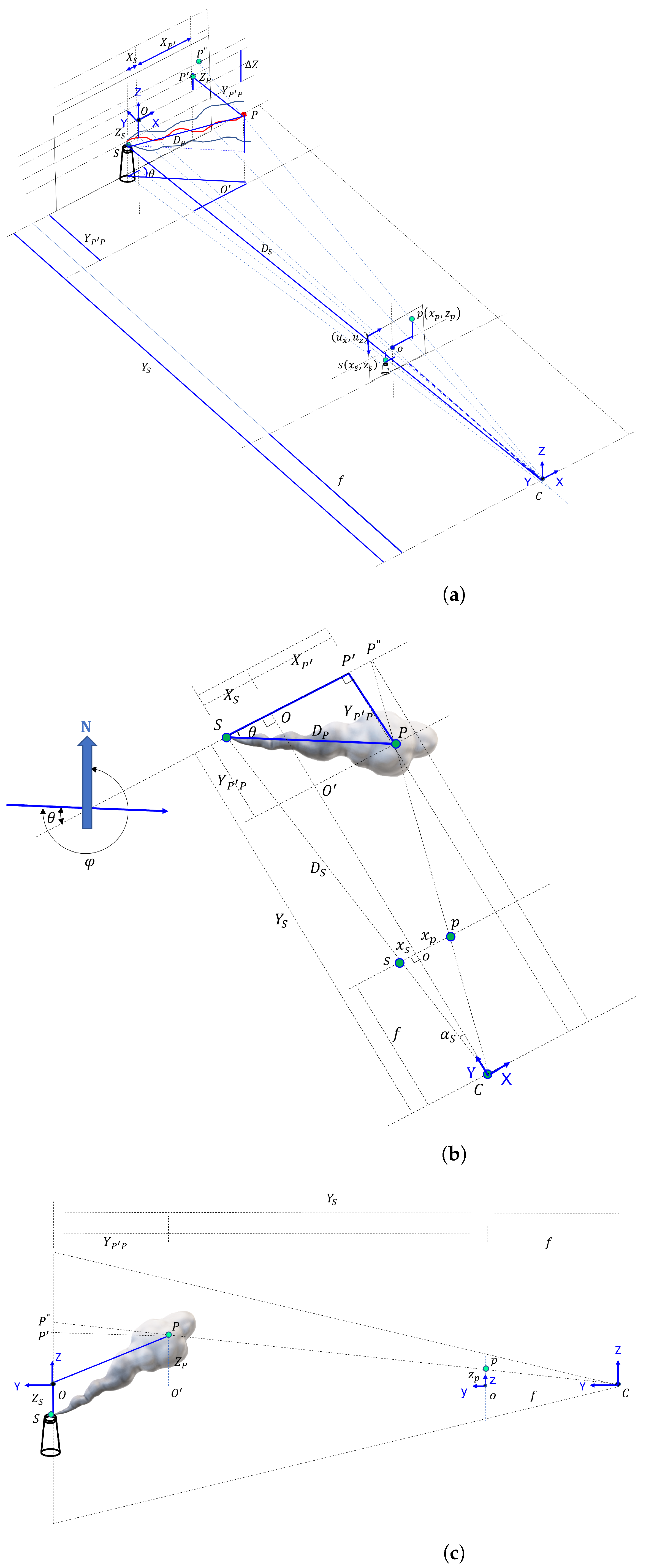
3.3. Geometric Transformation

The Geometric Transformation module shown in Figure 3 plays an important role in transferring the PR characteristics localized in a 2D image predicted by DPRNet to their corresponding positions in 3D world coordinates. The PC characteristics that we have been interested in 2D-to-3D transformation are the PR and the PR distance. Figure 4 shows a schematic diagram explaining the geometry of the PC characteristics shown in a camera view and its orthographic view. Figure 7 shows the geometry of the PC characteristics with respect to a camera in 3D (Figure 7a) and 2D top view (Figure 7b) and 2D side view (Figure 7c). As shown in Figure 7a, the PR distance, $D_P$, is a distance measured between S and P on a horizontal plane made by two vectors, an optical axis, $CY$, and its orthogonal vector, $CX$, where C represents the camera center’s position in the world coordinate and $(X,Y,Z)$ are the world coordinate vectors. Figure 7c defines the PR, $\Delta Z$, which is an effective height measured between the smokestack’s exit point, S, and the NBP, P.

In this study, we assume that several parameters are known in advance. The distance between the camera and the position of the smokestack, $D_S$ in Figure 7b, measured by Google Maps (https://maps.google.com, accessed on 1 January 2022), a web-based service providing detailed information about geographical regions and sites worldwide, is already known. Given the geographical location information about the camera and the smokestack, we measured $D_S$ using Google Maps. In addition, we assume that the information about the wind direction is pre-known. For instance, $\phi ={90}^{\circ }$ is wind from the east, and $\phi ={180}^{\circ }$ is wind from the south. Based on the camera’s position, capturing desired smokestack images, and geographical directions, wind direction relative to the image plane can be obtained as $\theta =|\phi -252|$ in this study. Finally, the camera’s intrinsic parameters, such as focal length, f, principal point’s position, o and extrinsic camera parameters, including camera position with respect to the origin of the world coordinates, are shown in Figure 7 and Figure 8.

With the known f and $D_S$, we can compute the position of the smokestack exit point S in the world coordinates. First, we can derive a geometric relationship between $(x_s,y_s)$ and $(X_S,Y_S)$ or $(x_s,z_s)$ and $(X_S,Z_S)$ using similarity triangle theorem with $\Delta COS$ and $\Delta Cos$ in Figure 7b,c, respectively, [59].

$$X_S=Y_S\frac{x_s}{f}$$

(6)

$$Z_S=Y_S\frac{z_s}{f}$$

(7)

Using the trigonometry theorem with $\Delta Cos$ and $\Delta COS$ in Figure 7b, we can also compute the horizontal angle of the smokestack, ${\alpha }_s$, and Y distance of the stack exit point, S, as below:

$${\alpha }_s={tan}^{-1}\frac{x_s}{f}$$

(8)

$$Y_S=D_{S}cos{\alpha }_s$$

(9)

Thus, we can calculate the position of the smokestack exit point, S, from $\Delta COS$ in Figure 7b, and Equations (6) and (7) as follows:

$$X_S=D_S\frac{x_s}{f}cos{\alpha }_s$$

(10)

$$Z_S=D_S\frac{z_s}{f}cos{\alpha }_s$$

(11)

Similarly, we can compute the position of the PR point, P. From $\Delta SP{P}^{{}^{\prime }}$, we can calculate the following:

$$tan\theta =\frac{Y_{P^{{}^{\prime }}P}}{X_S+X_{P^{{}^{\prime }}}}$$

(12)

Since two triangles, $\Delta Cop$ and $\Delta C{O}^{{}^{\prime }}P$, are similar, we can derive:

$$\frac{x_p}{X_{P^{{}^{\prime }}}}=\frac{f}{Y_S-Y_{P^{{}^{\prime }}P}}$$

(13)

Furthermore, since $\theta$ is given from the weather station, we can calculate $X_{P^{{}^{\prime }}}$ by substituting Equation (12) in Equation (13) as follows:

$$X_{P^{{}^{\prime }}}=\frac{Y_S-X_{S}tan\theta }{\frac{f}{x_p}+tan\theta }$$

(14)

$$Y_{P^{{}^{\prime }}P}=\frac{X_{S}f-Y_S{x}_p}{fcot\theta +x_p}$$

(15)

Furthermore, we can compute the following PR ratio from Figure 7c:

$$\frac{z_p}{Z_P}=\frac{f}{Y_S-Y_{P^{{}^{\prime }}P}}$$

(16)

Thus, the PR height, $Z_P$, can be calculated as below:

$$Z_P=\frac{Y_S-Y_{P^{{}^{\prime }}P}}{f}{z}_p$$

(17)

By substituting Equations (9) and (15) in Equation (17):

$$Z_P=\frac{z_p}{f}\frac{D_{S}cos{\alpha }_{s}sin\theta -X_{S}cos\theta }{\frac{x_p}{f}cos\theta +sin\theta }$$

(18)

Therefore, PR and PR distance can be calculated as follows:

$$\Delta Z=|Z_S-Z_P|$$

(19)

$$D_P=\sqrt{{(X_S+X_{P^{{}^{\prime }}})}^2+Y_{P^{{}^{\prime }}P}^2}$$

(20)

4. Experimental Results and Discussion

In this section, we discuss our image datasets and the industrial area from which these datasets were collected and shared. Additionally, we will explain the validation metrics used to compare our proposed method to other competitive methods in smoke border detection and recognition. Our discussion then proceeds to the two final sections, titled “Comparison with existing smoke recognition methods” and “Plume rise measurement”, where the performance of the proposed method is evaluated, and the PR is calculated based on our “DPRNet”, respectively. To validate the performance of our proposed method, we used a computer equipped with a Core i9, 3.70 GHz/4.90 GHz, 20 MB cache CPU, 64 GB RAM, and an NVIDIA GeForce RTX 3080, 10 GB graphics card. The total training time for the network was approximately one hour, utilizing Python 3.8 with the PyTorch Deep Learning framework. Finally, for geometric transformation and image processing analysis, we employed MATLAB R2022b software.

4.1. Site Description

The imaging system was deployed on a meteorological tower with a clear sightline to the desired smokestack operated by the Wood Buffalo Environment Association (WBEA). It is located outside the Syncrude oil sands processing facility north of Fort McMurray, Alberta, Canada. Figure 10 represents the satellite images, the location of the camera, and the desired smokestack.

WBEA operates a 10-meter-tall meteorological tower with a clear sightline to the smokestacks (

Table 1. Syncrude smokestacks information, including location, smokestack height ($h_s$), smokestack diameter ($d_s$), the effluent velocity at the smokestack exit (${\omega }_s$), and effluent temperature at the smokestack exit ($T_s$). The velocities and temperatures are averages for the entire capturing period.

Reported ID	Latitude	Longitude	${\mathit{h}}_{\mathit{s}}$ (m)	${\mathit{d}}_{\mathit{s}}$ (m)	${\mathit{\omega }}_{\mathit{s}}$ (${\mathbf{ms}}^{-1}$)	${\mathit{T}}_{\mathit{s}}$ (K)
Syn. 12908	57.041	−111.616	183.0	7.9	12.0	427.9
Syn. 12909	57.048	−111.613	76.2	6.6	10.1	350.7
Syn. 13219	57.296	−111.506	30.5	5.2	8.8	355.0
Syn. 16914	57.046	−111.602	45.7	1.9	12.0	643.4
Syn. 16915	57.046	−111.604	31.0	5.0	9.0	454.5
Syn. 16916	57.297	−111.505	31.0	5.2	9.2	355.0

) at the south of the Syncrude facility (https://wbea.org/stations/buffalo-viewpoint, accessed on 1 January 2022). The camera system is mounted on this tower above the tree canopy, as they are on a hill sloping downward from the tower location, and the largest smokestack and its PC are always visible. The system consists of a digital camera with shutter control and a camera housing for weather protection, including interior heating for window defrost and de-icing.

The Syncrude processing facility has six main smokestacks, tabulated in Table 1. The tallest one is approximately 183 m, and the heights of the other five range from 31 m to 76 m. To isolate a single smoke plume rise, we have focused on the area’s tallest one, which can help find the PR for one plume source. Wind directions during the capturing period were determined from the Mildred Lake Air Monitoring Station (https://wbea.org/stations/mildred-lake, accessed on 1 January 2022), located at the Mildred Lake airstrip (AMS02: Latitude: $57.{05}^{\circ }$, Longitude: $-111.{56}^{\circ }$), approximately 5 km from the Syncrude facility.

4.2. Deep Plume Rise Dataset (DPRD)

The greatest challenge in using deep learning for PC recognition is the lack of annotated images for training. Therefore, creating image datasets for PC recognition for research and industry purposes is invaluable. For this study, 96 images were captured daily; for the first part of the project, 35 K images were collected from January 2019 to December 2019. The collected images demonstrated various types of plume shapes in different atmospheric conditions. The dataset has been classified into day, night, and cloudy/foggy conditions. Cloudy/foggy conditions are assigned to images captured during low visibility conditions caused by clouds or fog. The collected dataset revealed that among 96 images captured daily, we have 48-day and 48-night images. There were some outlier images for different reasons, such as camera handle shaking, auto-focus problems, disturbing smoke, and severe snow and hail. Furthermore, some PCs could not be recognized from their background, even by visual image inspection. As a consequence, among 35 K collected images, 10,684 were valid. Note that about 8110 images were captured when the facility was not working.

This paper introduces a new benchmark, DPRD, including a 2500 annotated dataset. DPRD contains PC upper and lower borders, smokestack exit image coordinates, PC centerline, and NBP image coordinates. In total, 60% of DPRD is considered training data and 40% is used for validation and testing. Rows (a) and (b) in Figure 11 show sample images from the region and their corresponding ground truth, which are generated by the “Labelme” graphical image annotation tool at https://github.com/wkentaro/labelme, accessed on 1 June 2021. We tried to select images of different atmospheric conditions, such as clear daytime, nighttime, cloudy, and foggy, to represent the results of different situations.

4.3. Model Validation Metrics

The performance of the considered methods is assessed using accuracy, recall, precision, and F1 score metrics. These metrics are defined based on four values, True Positive (TP), True Negative (TN), False Positive (FP), and False Negative (FN), which are derived from the confusion matrix of each introduced method [60]. The accuracy validation metric represents the proportion of correctly predicted observations to the total number of observations. In our application, the model’s accuracy signifies the ability of our model to accurately recognize PC pixels. This criterion is valid as long as FP and FN values are roughly equal [60]. If not, alternative validation metrics should be taken into account. The foreground pixel coverage of the sample images can be seen in Figure 11, indicating that accuracy is not appropriate for this study. Recall, or sensitivity, is the ratio of correctly predicted positive observations to all actual positive observations. Recall demonstrates the number of PC pixels labelled among all the actual PC pixels. Recall is calculated as follows:

$$Recall=\frac{TP}{TP+FN}$$

(21)

Precision is the ratio of positive observations which are predicted correctly to all observations which are predicted as positive. This metric represents how many PC pixels exist among all the pixels labelled as PC. Therefore, a low rate of FP can achieve high precision. This validation metric is obtained as follows,

$$Precision=\frac{TP}{TP+FP}$$

(22)

As it is implied from Equations (21) and (22), precision and recall take either FP or FN into account. The last validation measure in this paper, the F1 score, considers both FP and FN as a weighted average of recall and precision metrics. Unlike accuracy, this metric is more useful when FP and FN are not the same as in our study. Our FP is less than FN, or the amount of non-actual PC pixels predicted as PC pixels is less than that of actual PC pixels predicted as non-PC pixels. Therefore, the F1 score helps us look at both recall and precision validation metrics as follows,

$$F1 score=\frac{2\times Recall\times Precision}{Recall+Precision}$$

(23)

4.4. Comparison with Existing Smoke Recognition Methods

In this section, we evaluate the performance of DPRNet and compare it with several competitors. To select suitable smoke recognition methods for comparison, we considered both the identification accuracy and computational complexity of the reviewed approaches, leading us to choose DeepLabv3+ [61], FCN [56], and regular Mask R-CNN. These methods have demonstrated good performance in object border detection and recognition tasks in previous studies and employ deep convolutional neural network architecture, effectively capturing and processing spatial features in the input image, resulting in improved accuracy in smoke border detection and recognition. Our proposed DPRNet is evaluated using three metrics introduced in Section 4.3.

As evident from

Table 2. Comparison of different methods for PC recognition using average validation metrics values.

Model	Recall	Precision	F1 Score
Mask R-CNN	0.556	0.727	0.607
FCN	0.591	0.859	0.599
DeepLabv3	0.654	0.892	0.721
DPRNet	0.846	0.925	0.881

, DPRNet outperforms competitive methods for 90 test images selected from various day, night, foggy, and cloudy conditions. Specifically, the recall and precision metrics highlight a significant difference between the models, demonstrating the effectiveness of the proposed model in recognizing actual PC pixels. The higher F1 score value for DPRNet compared to the competitors guarantees that DPRNet performs better than the other three methods, showcasing its efficacy. Among our competitive methods, DeepLabv3+ performed better in terms of all validation metrics, while Mask R-CNN had the worst performance.

In addition to these average values, the detailed statistics for each model are provided in Figure 12 concerning each validation metric used. At first glance, our proposed method exhibits the most robust performance in all situations. Among the competitors, Mask R-CNN and FCN have the worst performance, while DeepLabv3 has slightly better efficiency. It is also evident from Figure 12 that some competitors have validation metrics of zero. This indicates that these methods were unable to detect any PCs in the corresponding images. In other words, the model might have been trained on a specific data type, and, consequently, it might misclassify unfamiliar types of data, resulting in lower accuracy, recall, and other performance metrics.

To further validate our DPRNet performance, we compared the models over the day, night, and foggy and cloudy datasets using a variety of validation metrics, as shown in Figure 13. The number of test images in both figures is 90, as shown on the horizontal axis in Figure 12. While this figure shows the results for each test image, Figure 13 presents the average outcomes for each validation metric across all test datasets. Furthermore, as the vertical axis in this figure represents the average value, it does not contain any zeros. All methods, with the exception of Mask R-CNN, exhibit acceptable performance on day and night datasets. Even with night precision, FCN is better than our proposed method. However, as discussed in Section 4.3, this metric can only partially convey the merit of a model individually, and it needs to be analyzed with the F1 score. Our proposed DPRNet outperforms the other rival methods by recognizing roughly all of the PC pixels correctly. Most datasets are related to cloudy and foggy conditions and are frequently seen within image batches. The strength of our DPRNet is its robust performance in this case, which is of paramount importance in our application. The DPRNet could improve the recall metric by 66%, 58%, and 87% on average in cloudy and foggy conditions relative to FCN, DeepLabv3, and Mask R-CNN frameworks, respectively, which means that the proposed method is able to find the PC regions appropriately, using $L_S$. This capability produces high-quality image recognition with a more complicated mixture of PCs and the sky behind. These high recall values help us meet our research application requirement, in which we should identify the entire PC stream for PR distance measurement.

To demonstrate the qualitative results of the proposed method, we show some visual results to compare competitive methods. Figure 14 depicts these recognition results. The first two rows represent the input images and their corresponding ground truths, respectively, and the other rows give the output of different models. We tried to visualize samples from all classes such that the first two images are related to cloudy/foggy conditions, the second two are from the nighttime dataset, and the last two are obtained from our daytime dataset. It is observed that DPRNet outperformed the other methods by attaining high accuracy of PC localization and, consequently, correctly recognizing the desired smokestack PC.

4.5. Plume Rise Measurement

As discussed in Section 3, DPRNet gives PC border detection and recognition. Then, we take advantage of the NBP image coordinates and the wind direction information from the meteorological tower to obtain PR real-life measurements through geometric transformations. Figure 15 illustrates the asymptotic curve for four PC images and the automatically chosen point NBP, where the PC reaches neutral buoyancy. Apart from the PR and PR distance values of each sample PC, estimated by the proposed framework (tabulated in

Table 3. PR and PR distance values of each of the four PC images from Figure 15.

Image	Date	Time	$\mathit{\phi }$ (deg.)	$\mathit{\theta }$ (deg.)	$\mathbf{\Delta }\mathit{Z}$ (m)	${\mathit{D}}_{\mathit{P}}$ (m)
I1	08-Nov-19	18-00-13	12.16	−239.8	460	842
I2	09-Nov-19	15-00-13	3.46	−248.5	126	1707
I3	14-Nov-19	10-00-16	10.41	−241.6	338	1960
I4	16-Nov-19	11-00-12	10.83	−241.1	427	3143

), the averaged hourly measured wind directions at the image sampling times are given as prior information of this study. The primary aim of this study is to assess the accuracy of Briggs equations by utilizing the images. These realistic PR and PR distance values within an extended period are required for future work, where our scope is a comparative study, and we will use image-based measurements to test and verify the Briggs equations.

5. Conclusions

To measure the PR through remote sensing images, PC recognition is of the essence as the first step. In this regard, a novel deep learning-based method, inspired by the nature of the problem, is proposed in this paper to detect and recognize the PC accurately. In the next stage, image processing analysis is leveraged to extract the PC centerline. Afterward, the critical point of this curve is estimated, the y-component coordinate of which is equivalent to PR. Lastly, this image measurement is transformed into a real-life world under the geometric transformation stage. Experimental results indicate that the proposed method, DPRNet, significantly outperformed its rivals. This work also demonstrated that PR could be determined with a single-camera system and wind direction measurements, allowing further investigation and understanding of the physics of how buoyant PCs interact with their environment under different meteorological conditions. Researchers can gain new insights into the fundamental physical processes that drive PC behaviour by systematically varying these conditions and observing how the PC responds. In addition, the method may allow them to study the effects of various external factors on buoyant PC behaviour. The proposed strategy can be extended to a more comprehensive method through several advancements in future research:

• Generalizing DPRNet to predict the PC and PC centerline simultaneously.
• Reinforcing DPRNet to recognize multi-source PCs occurring in industrial environments.
• Conducting comparative studies using meteorological and smokestack measurements between the estimated PR and PR distance from the proposed framework and the Briggs parameterizations equations.
• Briggs parameterization modification via estimated PR and PR distance from the proposed framework.

References

1. Briggs, G.A. Plume rise predictions. In Lectures on Air Pollution and Environmental Impact Analyses; Springer: Berlin/Heidelberg, Germany, 1982; pp. 59–111. [Google Scholar]
2. Ashrafi, K.; Orkomi, A.A.; Motlagh, M.S. Direct effect of atmospheric turbulence on plume rise in a neutral atmosphere. Atmos. Pollut. Res. 2017, 8, 640–651. [Google Scholar] [CrossRef]
3. Briggs, G.A. Plume Rise: A Critical Survey; Technol Report; Air Resources Atmospheric Turbulence and Diffusion Lab.: Oak Ridge, TN, USA, 1969.
4. Briggs, G. Plume rise predictions, lectures on air pollution and environment impact analysis. Am. Meteorol. Soc. 1975, 10, 510. [Google Scholar]
5. Bieser, J.; Aulinger, A.; Matthias, V.; Quante, M.; Van Der Gon, H.D. Vertical emission profiles for europe based on plume rise calculations. Environ. Pollut. 2011, 159, 2935–2946. [Google Scholar] [CrossRef] [PubMed] [Green Version]
6. Bringfelt, B. Plume rise measurements at industrial chimneys. Atmos. Environ. 1968, 2, 575–598. [Google Scholar] [CrossRef]
7. Makar, P.; Gong, W.; Milbrandt, J.; Hogrefe, C.; Zhang, Y.; Curci, G.; Žabkar, R.; Im, U.; Balzarini, A.; Baró, R.; et al. Feedbacks between air pollution and weather, part 1: Effects on weather. Atmos. Environ. 2015, 115, 442–469. [Google Scholar] [CrossRef]
8. Emery, C.; Jung, J.; Yarwood, G. Implementation of an Alternative Plume Rise Methodology in Camx; Final Report, Work Order No. 582-7-84005-FY10-20; Environ International Corporation: Novato, CA, USA, 2010. [Google Scholar]
9. Byun, D. Science Algorithms of the Epa Models-3 Community Multiscale Air Quality (Cmaq) Modeling System; EPA/600/R-99/030; U.S. Environmental Protection Agency: Washington, DC, USA, 1999.
10. Rittmann, B.E. Application of two-thirds law to plume rise from industrial-sized sources. Atmos. Environ. 1982, 16, 2575–2579. [Google Scholar] [CrossRef]
11. England, W.G.; Teuscher, L.H.; Snyder, R.B. A measurement program to determine plume configurations at the beaver gas turbine facility, port westward, oregon. J. Air Pollut. Control. Assoc. 1976, 26, 986–989. [Google Scholar] [CrossRef]
12. Hamilton, P. Paper iii: Plume height measurements at northfleet and tilbury power stations. Atmos. Environ. 1967, 1, 379–387. [Google Scholar] [CrossRef]
13. Moore, D. A comparison of the trajectories of rising buoyant plumes with theoretical/empirical models. Atmos. Environ. 1974, 8, 441–457. [Google Scholar] [CrossRef]
14. Sharf, G.; Peleg, M.; Livnat, M.; Luria, M. Plume rise measurements from large point sources in israel. Atmos. Environ. Part A Gen. Top. 1993, 27, 1657–1663. [Google Scholar] [CrossRef]
15. Webster, H.; Thomson, D. Validation of a lagrangian model plume rise scheme using the kincaid data set. Atmos. Environ. 2002, 36, 5031–5042. [Google Scholar] [CrossRef]
16. Gordon, M.; Li, S.-M.; Staebler, R.; Darlington, A.; Hayden, K.; O’Brien, J.; Wolde, M. Determining air pollutant emission rates based on mass balance using airborne measurement data over the alberta oil sands operations. Atmos. Meas. Tech. 2015, 8, 3745–3765. [Google Scholar] [CrossRef] [Green Version]
17. Gordon, M.; Makar, P.A.; Staebler, R.M.; Zhang, J.; Akingunola, A.; Gong, W.; Li, S.-M. A comparison of plume rise algorithms to stack plume measurements in the athabasca oil sands. Atmos. Chem. Phys. 2018, 18, 14695–14714. [Google Scholar] [CrossRef] [Green Version]
18. Akingunola, A.; Makar, P.A.; Zhang, J.; Darlington, A.; Li, S.-M.; Gordon, M.; Moran, M.D.; Zheng, Q. A chemical transport model study of plume-rise and particle size distribution for the athabasca oil sands. Atmos. Chem. Phys. 2018, 18, 8667–8688. [Google Scholar] [CrossRef] [Green Version]
19. Isikdogan, F.; Bovik, A.C.; Passalacqua, P. Surface water mapping by deep learning. IEEE J. Sel. Top. Appl. Earth Obs. Remote Sens. 2017, 10, 4909–4918. [Google Scholar] [CrossRef]
20. Isikdogan, F.; Bovik, A.; Passalacqua, P. Rivamap: An automated river analysis and mapping engine. Remote Sens. Environ. 2017, 202, 88–97. [Google Scholar] [CrossRef]
21. Gu, K.; Qiao, J.; Lin, W. Recurrent air quality predictor based on meteorology-and pollution-related factors. IEEE Trans. Ind. Inform. 2018, 14, 3946–3955. [Google Scholar] [CrossRef]
22. Gu, K.; Qiao, J.; Li, X. Highly efficient picture-based prediction of pm2. 5 concentration. IEEE Trans. Ind. Electron. 2018, 66, 3176–3184. [Google Scholar] [CrossRef]
23. Gubbi, J.; Marusic, S.; Palaniswami, M. Smoke detection in video using wavelets and support vector machines. Fire Saf. J. 2009, 44, 1110–1115. [Google Scholar] [CrossRef]
24. Yuan, F. Video-based smoke detection with histogram sequence of lbp and lbpv pyramids. Fire Saf. J. 2011, 46, 132–139. [Google Scholar] [CrossRef]
25. Yuan, F. A double mapping framework for extraction of shape-invariant features based on multi-scale partitions with adaboost for video smoke detection. Pattern Recognit. 2012, 45, 4326–4336. [Google Scholar] [CrossRef]
26. Yuan, F.; Shi, J.; Xia, X.; Fang, Y.; Fang, Z.; Mei, T. High-order local ternary patterns with locality preserving projection for smoke detection and image classification. Inf. Sci. 2016, 372, 225–240. [Google Scholar] [CrossRef]
27. Yuan, F.; Fang, Z.; Wu, S.; Yang, Y.; Fang, Y. Real-time image smoke detection using staircase searching-based dual threshold adaboost and dynamic analysis. IET Image Process. 2015, 9, 849–856. [Google Scholar] [CrossRef] [Green Version]
28. Khan, S.; Muhammad, K.; Hussain, T.; Ser, J.D.; Cuzzolin, F.; Bhattacharyya, S.; Akhtar, Z.; de Albuquerque, V.H.C. Deepsmoke: Deep learning model for smoke detection and segmentation in outdoor environments. Expert Syst. Appl. 2021, 182, 115125. [Google Scholar] [CrossRef]
29. Shi, Y.-k.; Zhong, Z.; Zhang, D.-X.; Yang, J. A study on smoke detection based on multi-feature. J. Signal Process. 2015, 31, 1336–1341. [Google Scholar]
30. Yuan, C.; Liu, Z.; Zhang, Y. Learning-based smoke detection for unmanned aerial vehicles applied to forest fire surveillance. J. Intell. Robot. Syst. 2019, 93, 337–349. [Google Scholar] [CrossRef]
31. Filonenko, A.; Hernández, D.C.; Jo, K.-H. Fast smoke detection for video surveillance using cuda. IEEE Trans. Ind. Inform. 2017, 14, 725–733. [Google Scholar] [CrossRef]
32. Zen, R.I.; Widyanto, M.R.; Kiswanto, G.; Dharsono, G.; Nugroho, Y.S. Dangerous smoke classification using mathematical model of meaning. Procedia Eng. 2013, 62, 963–971. [Google Scholar] [CrossRef] [Green Version]
33. Wang, H.; Chen, Y. A smoke image segmentation algorithm based on rough set and region growing. J. For. Sci. 2019, 65, 321–329. [Google Scholar] [CrossRef] [Green Version]
34. Zhao, W.; Chen, W.; Liu, Y.; Wang, X.; Zhou, Y. A smoke segmentation algorithm based on improved intelligent seeded region growing. Fire Mater. 2019, 43, 725–733. [Google Scholar] [CrossRef]
35. Ajith, M.; Martínez-Ramón, M. Unsupervised segmentation of fire and smoke from infra-red videos. IEEE Access 2019, 7, 182381–182394. [Google Scholar] [CrossRef]
36. Dimitropoulos, K.; Barmpoutis, P.; Grammalidis, N. Higher order linear dynamical systems for smoke detection in video surveillance applications. IEEE Trans. Circuits Syst. Video Technol. 2016, 27, 1143–1154. [Google Scholar] [CrossRef]
37. Pham, H.N.; Dang, K.B.; Nguyen, T.V.; Tran, N.C.; Ngo, X.Q.; Nguyen, D.A.; Phan, T.T.H.; Nguyen, T.T.; Guo, W.; Ngo, H.H. A new deep learning approach based on bilateral semantic segmentation models for sustainable estuarine wetland ecosystem management. Sci. Total Environ. 2022, 838, 155826. [Google Scholar] [CrossRef]
38. Shi, B.; Patel, M.; Yu, D.; Yan, J.; Li, Z.; Petriw, D.; Pruyn, T.; Smyth, K.; Passeport, E.; Miller, R.D.; et al. Automatic quantification and classification of microplastics in scanning electron micrographs via deep learning. Sci. Total Environ. 2022, 825, 153903. [Google Scholar] [CrossRef]
39. Muhammad, K.; Khan, S.; Palade, V.; Mehmood, I.; Albuquerque, V.H.C.D. Edge intelligence-assisted smoke detection in foggy surveillance environments. IEEE Trans. Ind. Inform. 2019, 16, 1067–1075. [Google Scholar] [CrossRef]
40. Veerappampalayam Easwaramoorthy, S.; Jaehyuk, C.; Malliga, S.; Obuli Sai, N. Forest fire and smoke detection using deep learning-based learning without forgetting. Fire Ecol. 2023, 19, 9. [Google Scholar]
41. Huanjie, T.; Qianyue, D. An adaptive frame selection network with enhanced dilated convolution for video smoke recognition. Expert Syst. Appl. 2023, 215, 119371. [Google Scholar]
42. Liu, M.; Xie, X.; Ke, G.; Qiao, J. Simple and efficient smoke segmentation based on fully convolutional network. DEStech Trans. Comput. Sci. Eng. 2019. [Google Scholar] [CrossRef]
43. Jia, Y.; Du, H.; Wang, H.; Yu, R.; Fan, L.; Xu, G.; Zhang, Q. Automatic early smoke segmentation based on conditional generative adversarial networks. Optik 2019, 193, 162879. [Google Scholar] [CrossRef]
44. Yuan, F.; Zhang, L.; Xia, X.; Wan, B.; Huang, Q.; Li, X. Deep smoke segmentation. Neurocomputing 2019, 357, 248–260. [Google Scholar] [CrossRef]
45. Yuan, F.; Dong, Z.; Zhang, L.; Xia, X.; Shi, J. Cubic-cross convolutional attention and count prior embedding for smoke segmentation. Pattern Recognit. 2022, 131, 108902. [Google Scholar] [CrossRef]
46. Hwang, B.; Kim, J.; Lee, S.; Kim, E.; Kim, J.; Jung, Y.; Hwang, H. Automatic detection and segmentation of thrombi in abdominal aortic aneurysms using a mask region-based convolutional neural network with optimized loss functions. Sensors 2022, 22, 3643. [Google Scholar] [CrossRef] [PubMed]
47. Girshick, R. Fast r-cnn. In Proceedings of the IEEE International Conference on Computer Vision, Santiago, Chile, 7–13 December 2015; pp. 1440–1448. [Google Scholar]
48. Visscher, A.D. Air Dispersion Modeling: Foundations and Applications; John Wiley & Sons: Hoboken, NJ, USA, 2013. [Google Scholar]
49. Cimorelli, A.J.; Perry, S.G.; Venkatram, A.; Weil, J.C.; Paine, R.J.; Wilson, R.B.; Lee, R.F.; Peters, W.D.; Brode, R.W. Aermod: A dispersion model for industrial source applications. part i: General model formulation and boundary layer characterization. J. Appl. Meteorol. 2005, 44, 682–693. [Google Scholar] [CrossRef] [Green Version]
50. Turner, D.B.; Schulze, R. Atmospheric Dispersion Modeling: Trinity Consultants; Trinity Consultants Inc.,: Oakland, CA, USA, 2007; 408p. [Google Scholar]
51. Ji, S.; Xu, W.; Yang, M.; Yu, K. 3d convolutional neural networks for human action recognition. IEEE Trans. Pattern Anal. Mach. Intell. 2012, 35, 221–231. [Google Scholar] [CrossRef] [Green Version]
52. He, K.; Gkioxari, G.; Dollár, P.; Girshick, R. Mask r-cnn. In Proceedings of the IEEE International Conference on Computer Vision, Venice, Italy, 22–29 October 2017; pp. 2961–2969. [Google Scholar]
53. Albawi, S.; Mohammed, T.A.; Al-Zawi, S. Understanding of a convolutional neural network. In Proceedings of the 2017 International Conference on Engineering and Technology (ICET), Antalya, Turkey, 21–23 August 2017; pp. 1–6. [Google Scholar]
54. Chen, X.; Gupta, A. An implementation of faster rcnn with study for region sampling. arXiv 2017, arXiv:1702.02138. [Google Scholar]
55. He, K.; Zhang, X.; Ren, S.; Sun, J. Deep residual learning for image recognition. In Proceedings of the IEEE Conference on Computer Vision and Pattern Recognition, Las Vegas, NV, USA, 27–30 June 2016; pp. 770–778. [Google Scholar]
56. Long, J.; Shelhamer, E.; Darrell, T. Fully convolutional networks for semantic segmentation. In Proceedings of the IEEE Conference on Computer Vision and Pattern Recognition, Boston, MA, USA, 7–12 June 2015; pp. 3431–3440. [Google Scholar]
57. Rafae, G.C.; Paul, W. Digital Image Processing; Addison-Wesley Longman Publishing Co., Inc.: Boston, MA, USA, 1987. [Google Scholar]
58. Lothar, B. Introduction to the Operational Calculus; Elsevier & Business Media: Amsterdam, The Netherlands, 2013. [Google Scholar]
59. Luhmann, T.; Robson, S.; Kyle, S.; Harley, I. Close Range Photogrammetry: Principles, Techniques and Applications; Whittles Publishing Dunbeath: Dunbeath, UK, 2006; Volume 3. [Google Scholar]
60. Geoff, D. Pattern Recognition and Classification: An Introduction; Springer Science & Business Media: Berlin/Heidelberg, Germany, 2012. [Google Scholar]
61. Chen, L.-C.; Zhu, Y.; Papandreou, G.; Schroff, F.; Adam, H. Encoder-decoder with atrous separable convolution for semantic image segmentation. In Proceedings of the European conference on computer vision (ECCV), Munich, Germany, 8–14 September 2018; pp. 801–818. [Google Scholar]
Figure 1. The scheme of the proposed framework.
Remotesensing 15 03083 g001
Figure 2. Region proposal network. Red rectangles illustrate the proposal regions on the feature map of the input image.
Remotesensing 15 03083 g002
Figure 3. PR measurements system framework. x p and z p are the NBP coordinates in the image scale. Similarly, X P and Z P represent the NBP coordinates in the real-life scale. Δ Z and D P are PR and PR distance in real-life scale. The x z system is chosen for visualizing the PR measurements to be consistent with other studies in environmental science.
Remotesensing 15 03083 g003
Figure 4. PR, Δ Z ; PR distance, D P ; and NBP, P; on a sample image. θ represents the PC deviation due to the wind, and φ denotes the wind direction. Furthermore, S indicates the smokestack exit, C represents the camera position, and the blue line shows the PC centerline. (a) Camera view of the PC. (b) Schematic top view of the PC.
Remotesensing 15 03083 g004
Figure 5. DPRNet architecture. The supplemental modules are shown in green, and the dashed blue rectangle is dismissed in the inference time.
Remotesensing 15 03083 g005
Figure 6. Sample PC segments with eight boundary points.
Remotesensing 15 03083 g006
Figure 7. The schematic view of the region in the real-world coordinates. (a) 3D view; (b) Top view; (c) Side view.
Remotesensing 15 03083 g007
Figure 8. Smokestack location schemes. Smokestack exit, s; and image center, o. PC centerline is represented with a blue line, and NBP image coordinates are shown with p ( x p , z p ) and p ( x p , y p ) , respectively, in camera view and top view schemes. (a) Camera view scheme. (b) Top view scheme.
Remotesensing 15 03083 g008
Figure 9. NBP extraction framework. Dashed arrows show the output of each block. The red curve represents the centerline of the PC. The cyan and yellow lines, respectively, display the upper and lower boundaries of the PC. Green dashes demonstrate the asymptotic curve, and the magenta point is NBP.
Remotesensing 15 03083 g009
Figure 10. Imaging situation. Camera station, C; and smokestack position, S. The abc coordinate system is only for differentiating the side and camera views and is not used as a coordinate reference system. The dashed yellow line connects the camera position to the smokestack position. (a) Top view; (b) 3D view.
Remotesensing 15 03083 g010
Figure 11. Sample images (up) and their corresponding ground truth (down) from our DPR dataset are listed as (a) Clear daytime, (b,c) cloudy day, and (d,e) clear nighttime.
Remotesensing 15 03083 g011
Figure 12. Performance of different methods regarding some test images (a) recall, (b) precision, and (c) F1 score metrics.
Remotesensing 15 03083 g012
Figure 13. Detailed comparison of methods over three datasets employing (a) recall, (b) precision, and (c) F1 score metrics.
Remotesensing 15 03083 g013
Figure 14. Qualitative results of recognition tasks listed as: (a) Input image, (b) corresponding ground truth, (c) results of Mask R-CNN, (d) FCN, (e) results of DeepLabv3, and (f) results of DPRNet.
Remotesensing 15 03083 g014
Figure 15. DPRNet and image measurement results. In column (c), the red curve represents the meandering of the PC. The cyan and yellow lines, respectively, illustrate the upper and lower boundaries of the PC. Green dashes show the asymptotic curve; the magenta asterisk is NBP. (a) Input image; (b) DPRNet result; and (c) Image measurement.
Remotesensing 15 03083 g015