Article

Analysis of Short-Term Drought Episodes Using Sentinel-3 SLSTR Data under a Semi-Arid Climate in Lower Eastern Kenya

1
Department of Geophysics and Space Science, Institute of Geography and Earth Sciences, ELTE Eötvös Loránd University, Pázmány Péter Sétány 1/C, H-1117 Budapest, Hungary
2
Department of Humanities and Languages, Karatina University, Karatina P.O. Box 1957-10101, Kenya
3
Department of Meteorology, Institute of Geography and Earth Sciences, ELTE Eötvös Loránd University, Pázmány Péter Sétány 1/A, H-1117 Budapest, Hungary
*
Author to whom correspondence should be addressed.
Remote Sens. 2023, 15(12), 3041; https://doi.org/10.3390/rs15123041
Submission received: 16 May 2023 / Revised: 30 May 2023 / Accepted: 8 June 2023 / Published: 10 June 2023
(This article belongs to the Special Issue Advances in Thermal Infrared Remote Sensing)

Abstract

:
This study uses Sentinel-3 SLSTR data to analyze short-term drought events between 2019 and 2021. It investigates the crucial role of vegetation cover, land surface temperature, and water vapor amount associated with drought over Kenya’s lower eastern counties. Therefore, three essential climate variables (ECVs) of interest were derived, namely Land Surface Temperature (LST), Fractional Vegetation Cover (FVC), and Total Column Water Vapor (TCWV). These features were analyzed for four counties between the wettest and driest episodes in 2019 and 2021. The study showed that Makueni and Taita Taveta counties had the highest density of FVC values (60–80%) in April 2019 and 2021. Machakos and Kitui counties had the lowest FVC estimates of 0% to 20% in September for both periods and between 40% and 60% during wet seasons. As FVC is a crucial land parameter for sequestering carbon and detecting soil moisture and vegetation density losses, its variation is strongly related to drought magnitude. The land surface temperature has drastically changed over time, with Kitui and Taita Taveta counties having the highest estimates above 20 °C in 2019. A significant spatial variation of TCWV was observed across different counties, with values less than 26 mm in Machakos county during the dry season of 2019, while Kitui and Taita Taveta counties had the highest estimates, greater than 36 mm during the wet season in 2021. Land surface temperature variation is negatively proportional to vegetation density and soil moisture content, as non-vegetated areas are expected to have lower moisture content. Overall, Sentinel-3 SLSTR products provide an efficient and promising data source for short-term drought monitoring, especially in cases where in situ measurement data are scarce. ECVs-produced maps will assist decision-makers with a better understanding of short-term drought events as well as soil moisture loss episodes that influence agriculture under arid and semi-arid climates. Furthermore, Sentinel-3 data can be used to interpret hydrological, ecological, and environmental changes and their implications under different environmental conditions.

1. Introduction

As a naturally recurring hazard, drought depletes water resources on the Earth’s surface [1]. Hence, vulnerable regions are under risk of extreme water shortages, which leads to scarcity and inaccessibility of drinking water as well as rivers and streams shrinkage due to rainfall deficits compared to evapotranspiration due to extremely high temperatures [2,3]. In this regard, global climate change has shown a likelihood of extreme and severe drought events due to anthropogenic activities and increased carbon dioxide (CO2), which influences temperature, a critical climatic parameter in drought analysis [4,5]. Short- and long-term drought monitoring is essential for addressing water scarcity issues and maintaining food security for local populations. Drought classification falls under four categories: meteorological where the number of days experiencing precipitation is less than the specified threshold given by standardized Precipitation Index (SPI) for various months, e.g., SPI-3 which accounts for precipitation deficit with respect to the reference time of 3 months, agricultural drought which occurs when meteorological drought leads to a soil moisture deficit that limits water availability for crops, hydrological drought associated with the deficit and reduced surface water supply due to prolonged precipitation shortfall, and socioeconomic drought caused by reduced supply and increased demand of essential economic goods [6,7]. The periods of these droughts are region-specific—for example, deficiency by more than double the actual seasonal rainfall from mean deviation in India [6]. These drought categories are interrelated and impact various sectors of the global economy.
The accurate measurement of meteorological parameters is fundamental [8] for monitoring droughts and other climate-related disasters. In this regard, remote sensing has been proven to be a valuable tool for drought monitoring, land use, and land change mapping in regions with scarce, inaccurate, or unavailable meteorological data [9]. Optical and radar satellite missions such as Sentinel, ERS-1/2, and Landsat missions have gained momentum in recent studies by providing geospatial data to monitor soil moisture content, drought, urban sprawl, and agricultural dynamics [10]. Remote sensing data have been used in various applications—for instance, soil salinity modeling under arid and semi-arid climates [11] to archaeological site mapping [12]. In Afghanistan, Rousta et al. [13] applied Moderate Resolution Imaging Spectroradiometer (MODIS) and Tropical Rainfall Measuring Mission (TRMM) sensors to study drought impacts on vegetation. The study revealed that vegetation coverage in Afghanistan was too low during drought seasons. In Hungary, Landsat-8 OLI data have been used to create a regression model for soil salinity prediction [14].
In terms of geographical scope of Eastern African remote sensing studies, Borges et al. [15] found that a combination of Sentinel-1 and Sentinel-2 data for Savannah landcover mapping provides a more accurate classification in Tanzania. In Kenya, Baringo county, Ng et al. [16] used Sentinel data to detect changes in Prosopis and Vachellia spp. Sentinel-2-based classifications are reliable and can be improved by combining temporal information retrieved from spectral indices. Similarly, Cheng et al. [17] used PlanetScope and Sentinel-2 data to detect changes in vegetation phenology dynamics in Kapiti plains to understand climatic variability effects on Kenya’s rangeland.
Fewer studies have used Sentinel-3 data in various applications. For instance, a comparative study by Hunt et al. [18] showed promising results for meteorological variables using Sentinel-3A and Sentinel-3B. Smith et al. [19] investigated radiometry processing uncertainty using Sentinel-3A and Sentinel-3B data. Furthermore, Fierke et al. [20] found that Sentinel-2 MSI data have a high potential to monitor forest cover in Mount Kenya due to high temporal and spatial resolution. Nonetheless, limited research has been conducted using Sentinel-3 SLSTR to monitor drought in Kenya. Therefore, Sentinel-3 SLSTR data were processed and explored for drought monitoring in lower eastern counties of Kenya by extracting LST, FVC, and TCWV products. Essential climate variables (ECVs) have been applied in climate change monitoring-related phenomena, especially drought. As a key variable, FVC has been widely used for agricultural yield prediction, ecological monitoring, and drought assessment [21,22,23]. In this context, Yang et al. [24] indicated that FVC depicts increasing trends in the growing season and insignificant increasing trends in summer, while in some cases, a significant decrease is observed in the growing season. Mu et al. [25] used the Global Land Surface Satellite (GLASS) to investigate the FVC trend in major Chinese cities and quantify CO2 concentrations caused by urbanization [26]. In addition, land surface temperature (LST) is also a key component for monitoring agricultural drought worldwide at various scales. Cheng et al. [27] (2008) assessed the effect of land cover changes on air temperature and found a relationship between LST and spatial land-use patterns, which could be related to drought. The results showed LST influences on land since indices related to land are valuable in describing spatiotemporal patterns [28]. LST depicts a significant parameter for examining patterns in biodiversity, surface energy balance, climate variability, and influence on vegetation growth, agricultural production, and the water cycle [29,30,31]. As it influences vegetation growth and soil moisture, it has attracted scientists recently [32,33,34]. TCWV is the total gaseous water in a vertical column of the atmosphere (mm or kg/m2). It is derived from the visible red and near-infrared spectral range [35], and it is crucial for understanding hydrological processes. The primary water vapor sources are evaporation and transpiration, depending on the geographical weather conditions and spatiotemporal variability [36]. Lindstrot et al. [37] have reviewed various methodologies for retrieving TCWV from satellite data developed during the past decades, such as radar sensors, as they provide reliable information regarding moisture content.
Kenya relies majorly on agriculture for its economy, accounting for 30% of the Gross Domestic Product (GDP) [38]. A study by Wanyama et al. [39] indicated that under-developing countries face considerable challenges in ensuring food security due to the dependency of their economies on rainfed agriculture. Thus, climate change threatens agriculture and livelihoods and influences local environments due to varying land–atmosphere interactions. As lower eastern counties heavily rely on rainfed agriculture, they became vulnerable to these adverse effects of climate change, hence experiencing extreme drought episodes in the recent past [40]. Moreover, eastern Kenya is characterized by physical and economic water scarcity, recurring crop failures with a low adaptive capacity, and resilience to extreme weather conditions. Therefore, this study explores short-term drought episodes using Sentinel-3 SLSTR data in lower eastern counties of Kenya. The aims are to (i) analyze and interpret Sentinel-3 SLSTR derived ECVs (LST, FVC, and TCWV) between wet and dry seasons; (ii) investigate Sentinel-3A SLSTR data usefulness in short-term moisture variation between 2019 and 2021; (iii) and investigate the association between soil moisture and short-term drought in eastern Kenya.

2. Materials and Methods
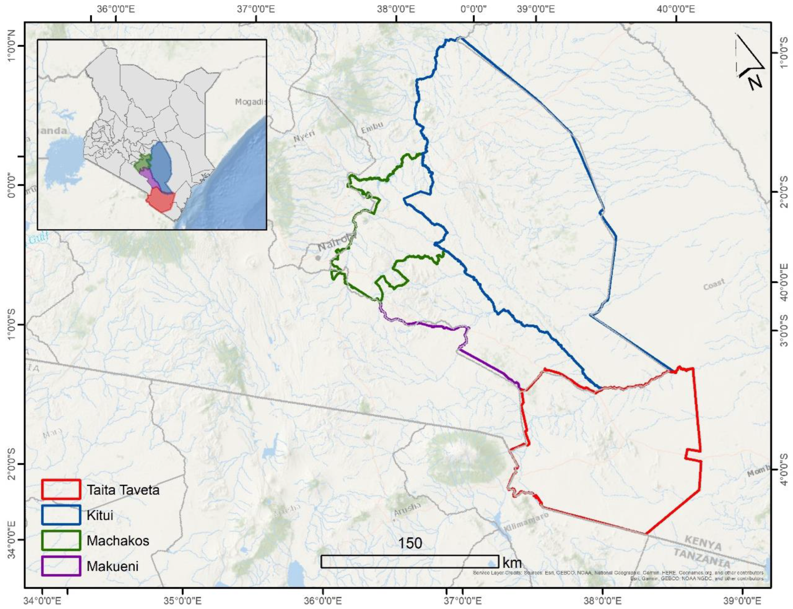
2.1. Study Area

Kenya lies between latitudes 5°N and 5°S and longitudes 34°E and 42°E in eastern Africa, occupying a total area of 582,646 km2. It has a population of 47,564,296 million per the 2019 census [41]. Around 89% of Kenya’s total landmass (29 out of 47 counties) is considered arid and semi-arid [42]. The rainfall distribution in Kenya is bimodal, with a mean annual precipitation of 669 mm and a mean temperature of 24.3 °C [43]. The short rainy season falls between October and December (OND) and is mainly influenced by the Inter-tropical Convergence Zone (ITCZ) [44]. The long rainy season falls between March and May (MAM) and is characterized by southeast trade and the Indian Monsoon winds [44]. Kenya has experienced various climate extremes, including droughts, floods, landslides, and forest fires, leading to the death and displacement of people, epidemics, property destruction, and forest loss [45]. These extreme climatic events are likely to increase and threaten local communities due to the projected temperature increase of 1 °C to 3.5 °C by 2050 [46,47].
The investigated areas are located in Eastern Kenya, namely Machakos, Makueni, Kitui, and Taita Taveta, as shown in Figure 1. Machakos county lies between latitudes 0°45′S and 1°31′S and longitudes 36°45′E and 37°45′E, with an area of 6208.2 km2 and a population of 1,421,932 [41]. It falls under arid and semi-arid climates, with an elevation ranging from 400 m to 2100 m above sea level [48]. The annual mean surface temperature varies between 18 °C and 29 °C. It receives an annual average rainfall of 500 mm to 1300 mm [49] and is characterized by a bimodal rainfall where short rains fall in OND, and long rains fall in MAM. Machakos is also distinct by variable and unpredictable rainfall rates [50]. The Kamba tribe predominantly occupies it. The county practices subsistence farming of maize and drought-resistant crops such as sorghum, millet fruits, and vegetables.
Makueni county lies between latitudes 1°35′ and 3°00′S and longitudes 37°10′ and 38°30′E. It has a landmass of 8034.7 km2 and a population of 987,653 [41]. It falls under an arid to semi-arid climate, characterized by severe water scarcity [2], food insecurity, and a lack of adaptability and resilience to climate change [44]. Makueni receives inadequate rainfall rates in relatively high areas ranging between 800 mm and 1200 mm, while low-lying areas receive low rainfall between 150 mm and 650 mm. As drought events with varying magnitudes frequently occur [2], the inhabitants suffer from crop yield decreases, especially maize [49]. Inhabitants look for alternative livelihood adaptation and mitigation strategies such as sand harvesting, which risks water access and availability [51].
Kitui county is located between latitudes 0°10′S and 3°0′S and longitudes 37°50′E and 39°0′E. It is characterized by a semi-arid climate, poorly distributed rainfall rates, and an altitude between 400 m and 1830 m above sea level [52]. It has a dense population of 1,136,187, with an annual growth rate of 2.2% [39]. The area is dominated by hilly landscapes such as Mutitu and Yatta plateaus [53], with a precipitation rate between 500 mm and 1050 mm [54]. Dominant crops include maize, sorghum, millet, pigeon, and peas.
Taita-Taveta county lies between latitudes 2°46′S and 4°10′S and longitudes 7°36′E and 30°14′E, with a total area of 17,084 km2. It has a semi-humid to semi-arid climate with a mean annual rainfall of 650 mm, an average annual temperature of 23 °C, and an average altitude of 596 m. It has a population of 340,671 [41], with agriculture as its primary livelihood source. The county receives an average rainfall of between 800 mm and 1200 mm per year, while low-lying areas receive an average of 150 mm to 650 mm. Taita-Taveta experiences a bimodal rainfall characterization [55,56].

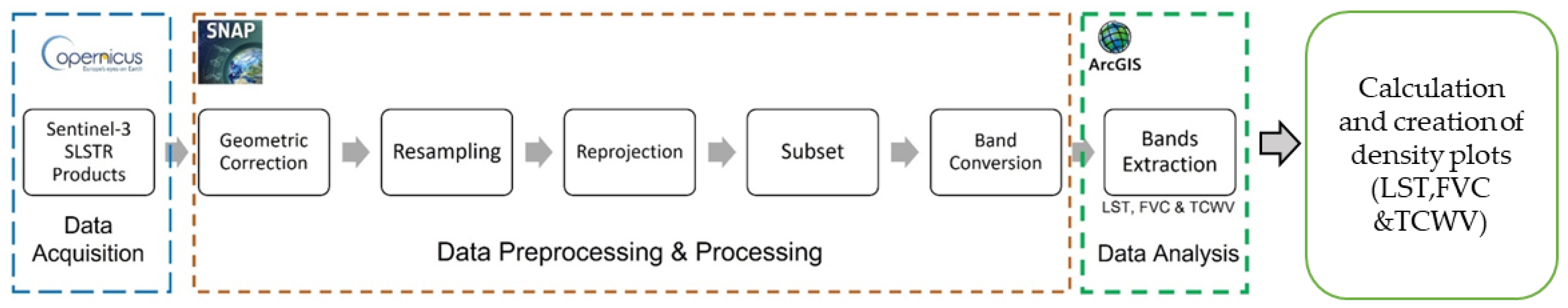
2.2. Sentinel-3 SLSTR Data

SLSTR, referring to the Sea and Land Surface Temperature Radiometer, is a dual scan temperature radiometer operating for the ESA Sentinel-3 mission in low Earth orbit as a part of the Copernicus Programme [57]. As the successor of the (A)ATSR mission series, SLSTR offers a wide range of applications related to Earth observation, the most prominent of which is Sea Surface Temperature (SST) assessment and land monitoring [58,59]. In addition, the instrument’s unique technological capabilities enable it to be used for fire detection [60]. It should also be highlighted that SLSTR contributes to climate change studies by providing the scientific community with Essential Climate Variables (ECVs), which are the focus of this study.
SLSTR products offer highly accurate global and regional Sea and Land Surface Temperatures (SST and LST) for climatological and meteorological applications. In this context, four Sentinel-3 SLSTR Level-2 LST products were downloaded from the Copernicus Open Access Hub. Sentinel-3 SLSTR product generates land surface parameters with a one km spatial resolution. It includes a measurement file with computed (i) Land Surface Temperature (LST) values for each pixel, associated with ancillary parameters, namely (ii) Normalized Difference Vegetation Index (NDVI), (iii) Glob Cover surface classification code (biome), (iv) Fractional Vegetation Cover (FVC), and (v) Total Column Water Vapor (TCWV). For more details, the Sentinel-3 SLSTR user guide contains an extended description of the mission’s products and properties of the SLSTR instrument [57].
This study sought to analyze and detect ECVs seasonal changes within three years since data for long-time detection requires high storage capacity and processing performance. Since April is the wettest month, and September is the driest month in Kenya [61], Sentinel-3 SLSTR data were acquired for four dates: April 2019, September 2019, April 2021, and September 2021. Specifically, the choice to focus on the months of April and September in Kenya was due to the fact that they are the rainiest and driest months, respectively. As a result, our selection process involved acquiring only one image per month. To ensure the highest quality data, we established a cloud cover criterion of less than 10% for the entire product scene. Data processing involved geometric correction and reprojection to WGS 84/UTM 37 S. Then, LST, TCWV, and FVC features were extracted from each product. It is worth noting that LST values were converted from Kelvin to Degrees Celsius (°C) using the band math tool in Sentinel Application Platform (SNAP). The products were resampled, stacked, and subset using vector data of Kenya’s administrative borders on the county level. In SLSTR Level-2 processing, FVC climatology specified as a fractional vegetation (F.V) index has a maximum value of one, which corresponds to 100% vegetation, and a minimum value of zero, which corresponds to 0% vegetation. Remotely sensed data properties are summarized in Table 1. Figure 2 summarizes the processing workflow of Sentinel-3 SLSTR data.
The description of the properties of the Sentinel-3 SLSTR level-2 products are as follows: the product ID is the datatake_ID which identifies univocally a given datatake. Shows the product details, the image details, and the Datatake time (a continuous acquisition of an image from Sentinel satellite in a given imaging mode). This further describes the compact naming convention which is arranged in the format, MMM_MSIXXX_YYYYMMDDHHMMSS_Nxxyy_ROOO_Txxxxx; where the first date (YYYYMMDDHHMMSS) is the datatake sensing time, and the second date is the “<Product Discriminator>” field, which is 15 characters in length and used to distinguish between different end-user products from the same datatake. S3B_SL_2_LST refers to Sentinel 3B satellite platform, Sentinel 3B level 2 product, and LST (Land surface temperature) is the product. Nxxyy is the Processing Baseline number (e.g., NT_004), ROOO is the Relative Orbit number, and Txxxxx is the Tile Number field. The sensing date refers to the date the satellite image was acquired [57]. S3B and S3A are twin satellites of the same mission, and they have the same instruments and properties.
Furthermore, we used ‘Create Random Points’ tool in ArcMap 10.3 to randomly generate a sample of 50,000 points from the entire region of interest to establish a correlation between ECVs. Once samples with null values were omitted, only 44,747 sampling points were left. LST, FVC, and TCWV were then compared, and a correlation analysis was performed using python code. Density plots were created to observe and visualize the distribution and correlation of ECVs. The process was performed for each period from dry to wet season by extracting corresponding ECVs values for samples.

2.2.1. Land Surface Temperature

The radiative temperature of the land in bare soil conditions and the effective emitting temperature of vegetation as determined from a top-view of a canopy determined by infrared radiation are referred to as Land Surface Temperature (LST) [62,63]. While local modeling relies significantly on field data, remote sensing has become the primary source for LST estimation at different scales [64,65,66,67]. The Radiative Transfer Equation (RTE) can be applied to a given thermal IR band to convert radiance observed at a sensor into Land Surface Temperature using Equation (1) [68].
L sensor =   τ ε L Ts +   L u +   τ     1   ε L d
where Lsensor is the top-of-atmosphere radiance; LTs is the radiance related to the surface temperature of a black object as per Planck’s law; Ts is the LST; and Lu and Ld are the upwelling and downwelling atmospheric radiances, respectively. τ is the atmospheric transmissivity, while ε is the land surface emissivity. Radiance is expressed in W∙sr −1∙m −2∙μm −1.

2.2.2. Fractional Vegetation Cover

The fraction of ground covered by green vegetation is known as the Fraction of Vegetation Cover (FVC). The FVC measures the spatial extent of vegetation without considering the canopy’s multi-layer properties [69]. It is an excellent option for replacing traditional vegetation indices in ecological monitoring due to its independence from illumination direction and sensitivity to canopy density [70]. Few studies have been conducted to estimate fractional vegetation based on optical remote sensing systems [71,72], yet the Normalized Difference Vegetation Index (NDVI) and the Scaled Difference Vegetation Index (SDVI) are the main methods being used. Both approaches take advantage of the differences in soil and vegetation properties at red and near-infrared (NIR) wavelengths [64]. The statistical relationships between the NDVI and the FVC are more suited to outlining a unique connection to estimate FVC as presented in Equation (2) [22].
FVC   = NDVI NDVI S NDVI V   NDVI S  
where NDVI is a weighted average of the Normalized Difference Vegetation Index [73] between vegetated and non-vegetated areas. NDVIs is the Normalized vegetation difference index of bare soil, and NDVIv is the vegetation index of the total vegetation cover [74]. The selection of NDVIv and NDVIs significantly affects the inversion precision of FVC. NDVI values are selected based on cumulative histograms of the NDVIs values, while the maximum value of NDVI as NDVIv [75]. The range between NDVIs and NDVIv used to estimate FVC from NDVI ranged between zero (0) for bare soil/non-vegetated areas to one (1) for vegetated areas [76,77].

2.2.3. Total Column Water Vapor

Total column water vapor estimates the total gaseous water contained in a vertical column of the atmosphere. Due to its complex interaction with the atmosphere [78], assessing water vapor is essential in Earth’s energy and hydrological cycle, as well as climate change studies, since water is one of the most important greenhouse gases, trapping heat more than carbon dioxide [79]. It is also known as atmospheric water vapor, precipitable water vapor (PWAT), and total precipitable water vapor (TPW) [80,81]. Water vapor compensates for over 99.9% of atmospheric moisture, and it is the primary source of atmospheric energy that drives weather systems’ development in short periods and influences the climate on longer time scales [82]. Water vapor movement and its related latent heat of vaporization account for over half of all heat transport processes from the tropics to the poles [83]. In theory, the water vapor content of a vertical air column reaching the top of the atmosphere with a base of 1 m2 equals the amount of water if all water vapor is condensed. The most commonly used units are kg/m2, referring to the mass of condensed water, and mm, referring to the amount of water accumulated at the bottom [84]. Equation (3) illustrates the TCWV mathematical expression.
T C W V = 1 ρ w g P s 0 q p d p
where ρw is the water density, which is 1000 kg/m3; g refers to the gravitational acceleration (9.8 m/s2); q(p) is the mixing ratio (g/kg) of water vapor at pressure level p; and Ps is the surface air pressure in hPa.

3. Results and Discussion

The interpretation of these parameters extracted from Sentinel-3 SLSTR data was crucial because they are associated with short-term drought, as weather patterns are summarized in precipitation anomalies and soil moisture loss episodes across arid and semi-arid regions in this context. We compared the lower eastern counties’ maps of Kitui, Machakos, Makueni, and Taita-Taveta to comprehend changes in ECVs between 2019 and 2021 for April and September.

3.1. Analysis and Interpretation of ECVs Derived from Sentinel-3 SLSTR Data

The ECVs derived from Sentinel-3 SLSTR data were analyzed and interpreted based on the seasons, the wettest, and the driest seasons. These interpretations are critical since they are associated with precipitation variations which influence soil moisture content and directly influence agriculture in lower eastern counties under study. In addition, the interpretation and visualization of ECVs are fundamental for proper agricultural timing and decision-making on agricultural dynamics in the agriculturally dominant lower eastern region. The detailed analysis and interpretation of ECVs for each county, Kitui, Machakos, Makueni and Taita-Taveta respectively are as shown below(Figure 3, Figure 4, Figure 5 and Figure 6).

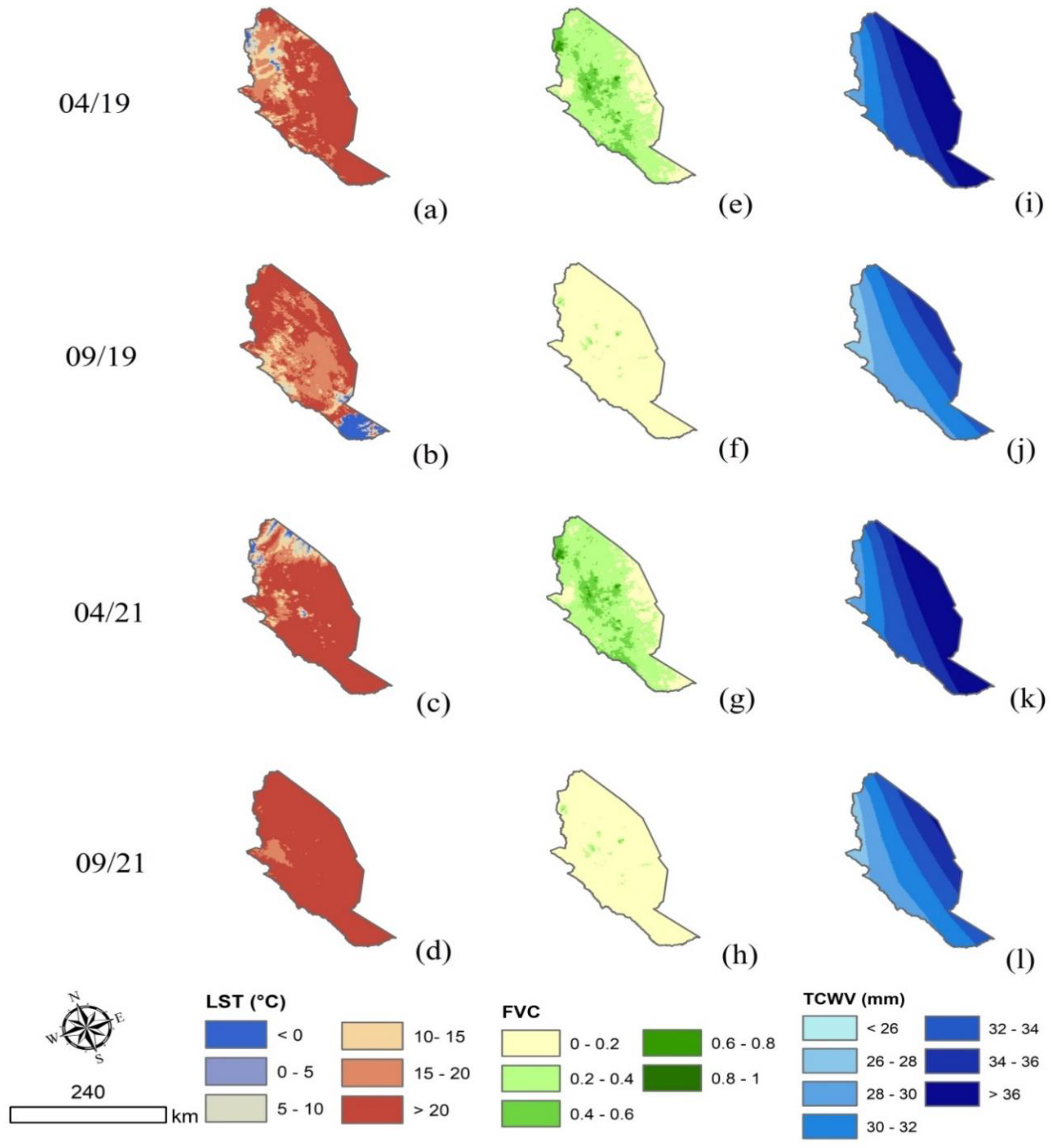
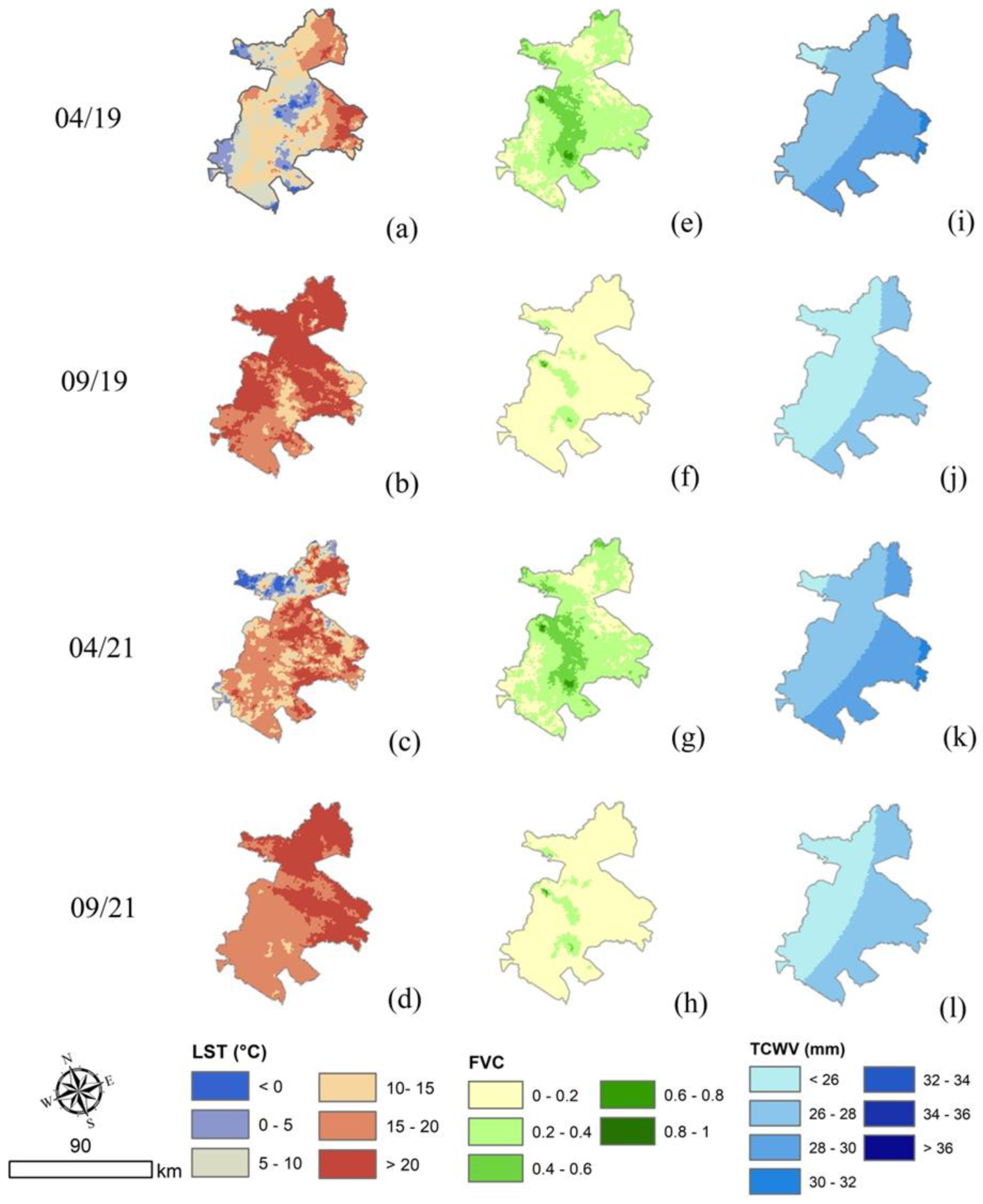
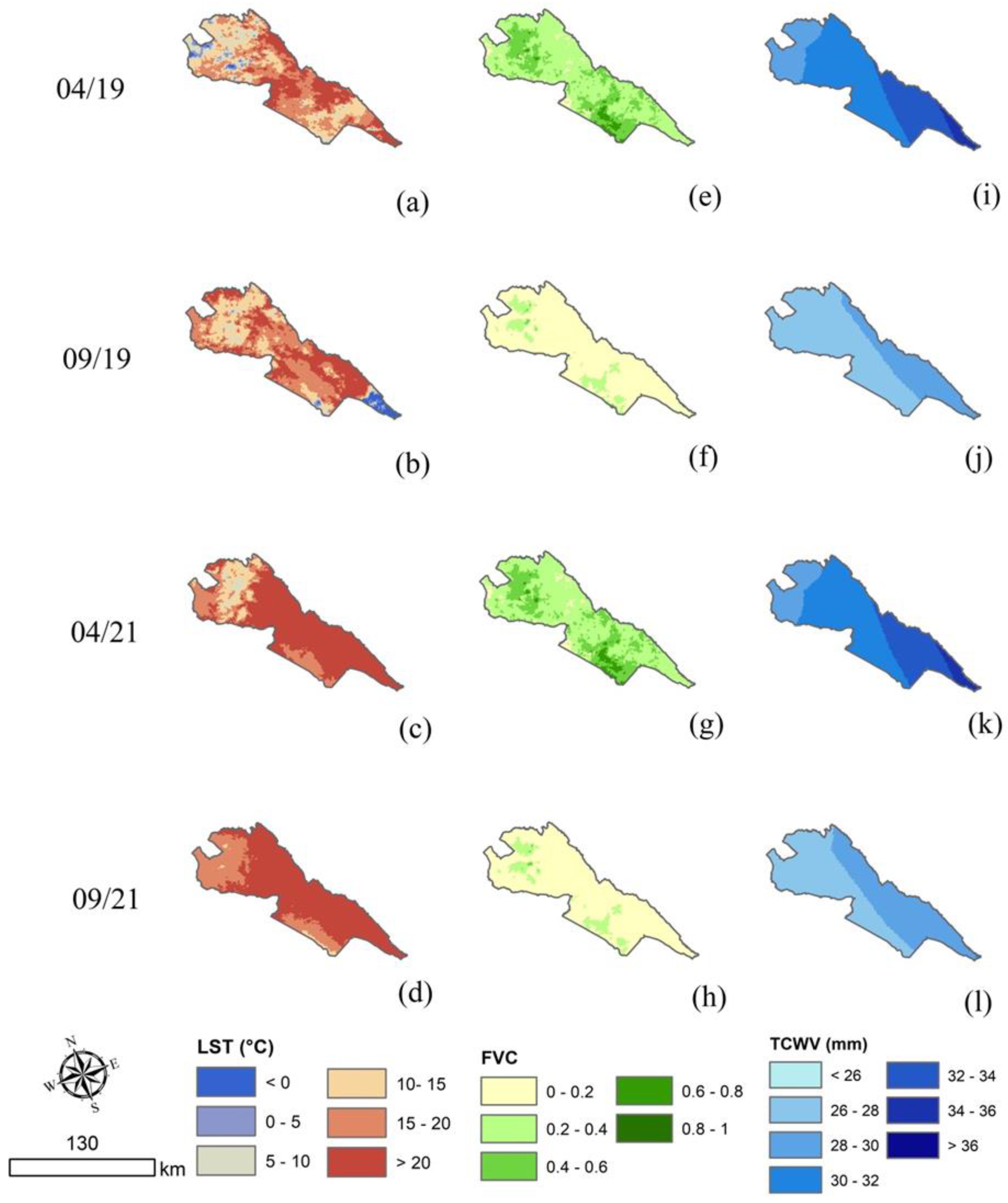
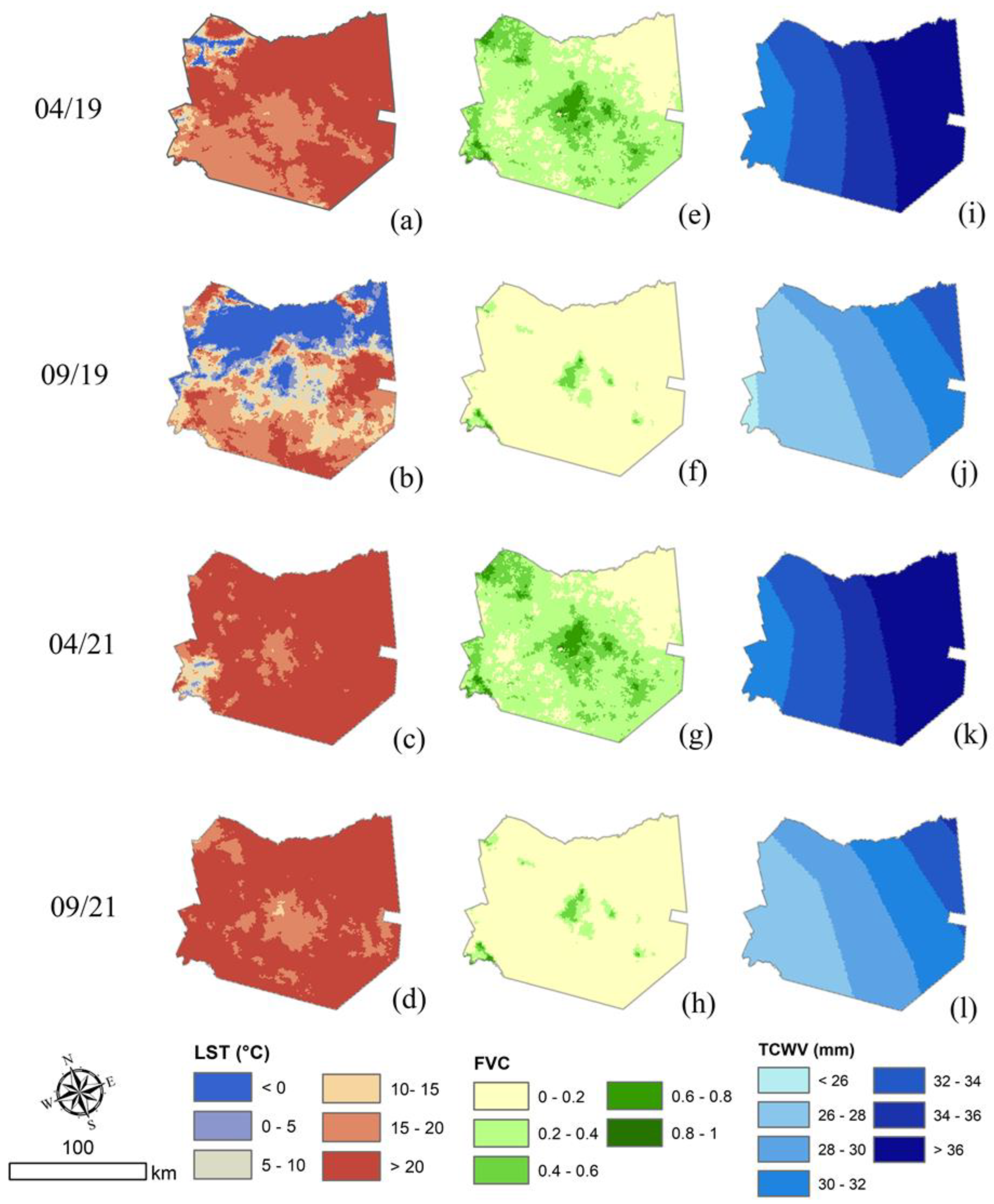
3.1.1. Land Surface Temperature (LST)

LST distribution in Eastern Kenya depicted varying spatiotemporal patterns. For Kitui county, Figure 3a–d shows that LST estimates for April 2019 were higher than 20 °C, except for a few locations with estimates ranging between 15 °C and 20 °C, while in Northern Kitui, estimates were relatively low, ranging between 0 °C and 5 °C. In April 2021, increased LST values were observed (above 20 °C), yet in the north, few areas had estimates between 0 °C and 5 °C. During the dry month of 2019, LST estimates were higher than 20 °C in the northern part of Kitui [85]. Mutunga et al. [53] found that the lowest annual average surface temperature varies from 14 °C to 22 °C, while the maximum annual average surface temperature ranges from 26 °C to 34 °C. In the center of Kitui, estimates vary between 15 °C and 20 °C, with a few areas with values between 10 °C and 15 °C. In the latter part, LST was underestimated (≤0 °C). On the other hand, LST estimates were greater than 20 °C, with a few areas having estimates between 15 °C and 20 °C. Overall, LST in Kitui county shows a slight increase during the wet and dry seasons of 2019 and 2021. Guha et al. [86] revealed similar patterns in India, with an average LST of 13.5 °C in the pre-monsoon, 12.3 °C in the monsoon, 8.8 °C in the post-monsoon, and 10.1 °C in the winter. Similarly, Mustafa et al. [33] showed that LST values over West Africa varied between 20.6 °C and 34.6 °C in 2010, 20.6 °C to 37.6 °C in 2018, and 21.2 °C to 38.7 °C in 2020, which is relatively consistent with the current study. Furthermore, LST increases are associated with changes in land cover from vegetated to non-vegetated surfaces [87], which can be used as an indirect drought indicator [33,88,89,90]. However, Sentinel-3 SLSTR has underestimated LST compared to in situ meteorological measurements in Kitui county.
Figure 4a–d show that LST estimates in April 2019 were generally low, with a few areas in the county having estimates of more than 20 °C in Machakos county. For April 2021, LST values slightly increased (>20 °C), but some locations had values ranging between 15 °C and 20 °C, which is consistent with the findings of Ahmed et al. [91]. For September 2019, LST estimates were greater than 20 °C, with the southern part having values ranging from 15 °C to 20 °C. In September 2021, most of the county had LST estimates between 15 °C and 20 °C, while the rest had values below 20 °C. In Makueni county, as shown in Figure 5a–d, LST estimates were greater than 20 °C in April 2019, except in a few locations with estimates ranging from below 0 °C to 15 °C. In April 2021, the LST estimates in the whole country were greater than 20 °C, while only a few areas recorded values between 15 °C and 20 °C. During the dry month of 2019, the southern part of Makueni had LST estimates below 0 °C. The rest of the county had LST estimates between 15 °C and 20 °C and greater than 20 °C. For September 2021, LST values were greater than 20 °C, with a few areas ranging between 15 °C and 20 °C. Like Kitui county, LST estimates in Makueni county are relatively low compared to in situ meteorological surface temperature, revealing an underestimation of LST by the sensor.
In Taita Taveta county, as illustrated in Figure 6a–d, LST values in April 2019 were greater than 20 °C, with a few areas in the county having estimates ranging from 15 °C to 20 °C. In the west, a few areas had estimates below 0 °C. Similar observations were found in April 2021, with almost the entire county experiencing high LST (>20 °C). In September 2019, LST estimates were the lowest in the northern part (below zero), with a few other areas varying from 0 °C to 5 °C, while other locations had LST estimates above 20 °C. For September 2021, it was observed that temperatures were higher (>20 °C), with a few areas having values from 15 °C to 2 °C. Based on LST maps, the temperature increased from 2019 to 2021 in dry and wet months, agreeing with Mwangi et al. [86]. This was caused by changes in vegetation density which were eventually influenced by increases in LST and reduction in soil moisture content [92].
The results implied variability in land cover among the four counties due to dense vegetation cover and land surface imperviousness in some areas. LST heterogeneity between the two seasons is caused by a slightly remarkable change in vegetation cover among the counties. This implies that LST influences agricultural yield and water availability, which depicts a significant challenge in the region. These interpretations are supported by Cui and de Foy [93], who revealed that LST seasonal variability depends on vegetation cover, weather parameters, and land surface characteristics. Previous studies found that LST is more significant in arid regions due to precipitation deficits [94], influencing soil moisture content and vegetation density across dry regions [95,96]. Furthermore, the findings of this study corroborate with [89,97,98] who used MODIS data and established that LST is a very essential component associated with the exchange of matter and energy between land and atmosphere as well as the change of ecological environment. LST also contributes to the study of drought monitoring [99,100]. Further, ref. [101] used MODIS data and indicated that the application of remote sensing helps to better understand the adverse effects of drought on crops and natural resources as implied by the study in context.

3.1.2. Fractional Vegetation Cover (FVC)

FVC is a reliable parameter to assess vegetation changes in response to drought on multiple scales. It corresponds with the partition between soil and vegetation contribution for emissivity and temperature. This property describes land surface processes used for climate and weather forecasting, natural hazards monitoring and prediction, as well as vegetation-soil dynamics monitoring and monitoring drought events in a given region [102]. Results from Kitui county, as shown in Figure 3e–h, indicate that FVC estimates ranged between 0 and 20% in September 2019 and 2021. A few areas had FVC between 20% and 40%. This implies reduced FVC estimates during the dry seasons, where short-term monthly droughts are experienced, affecting soil moisture content in the county. These findings imply food insecurity in the county due to immature crops because insufficient precipitation has worsened the existing food and water shortages across the region. The county as well as the whole of lower eastern Kenya has faced four consecutive poor rainy seasons for the last four years, exacerbating the adverse effects of the drought—for example, death of livestock, malnutrition, and mass agricultural crop failure that support subsistence farming in the region. For April 2019, FVC in a few areas varied between 60% and 80%. Forests are continually under threat of deforestation, such as the cases of the Museve forest and Mutuluni forest located in Kitui Central and Eastern Kitui [103]. The United Nations Environment Programme indicated that most forests in arid and semi-arid regions are scattered around hilltops and nature reserves [104]—for instance, in the highlands of Migwani, Mumoni, Kitui Central, Mui, Mutitu Hills, and Yatta plateau [81] where they play a primary role in ecological sustainability.
A significant part of the county had moderate estimates of 20% to 60% of FVC, yet some areas had a minimum of 0% to 20%. The same pattern was observed in April 2021, but it was noticeable that the FVC estimates were lower compared to 2019. These results implied that the precipitation received in April 2021 was lower compared to April 2019, as low precipitation is attributable to low soil moisture content, hence the low FVC values. This finding implies the importance of precipitation for water availability, food security, and stability in the region in the current context of climate change. This observation corroborates with [39,105,106], who stated that vegetation growth follows precipitation patterns and varies depending on vegetation types. In Machakos county, as presented in Figure 4e–h, results indicated that FVC estimates ranged from 40% to 60% in April 2019 and 2021, except in a few areas whose values fall between 0% and 20% and between 60% and 80%. Presumably, vegetation density gradually decreased from 2019 to 2021. In September 2019 and 2021, the FVC pattern was similar, with values ranging from 0% to 20%, while a few areas had values ranging from 20% to 40%. The results of Makueni county, as presented in Figure 5e–h, indicate that FVC estimates mostly ranged between 40% and 60% in April 2021. Yet only a few areas had FVC estimates greater than 60%. Nevertheless, some estimates were more significant than 20% in a few areas. For April 2021, FVC estimates ranged from 40% to 60% and between 60% and 80% in a few cases. Similar findings of vegetation densities range from 0% to 20% (Low density), 40–60% (Medium density), and 60–80% (High density) [107,108]. In our study, it is noticeable that there was a gradual reduction in FVC estimates from 2019 to 2021. A study by Xie et al. (2022) [109] observed a change in vegetation cover for the Ulan Buh desert in western inner Mongolia using RGB data and pixel-based machine learning methods area. There was a significant change from 2006 to 2019, with an increase in grass coverage from 15.47 ± 1.49% to 27.90 ± 2.79%, an indication of RGB images’ suitability in mapping FVC. Similarly, our methodology is equally suitable in detecting changes in vegetation cover since between September 2019 and 2021, vegetation density ranged between 0% and 20%, with only a few areas having values between 20% and 40%. This implies the feasibility of remote sensing data such as vegetation monitoring as well as short-term droughts analysis in lower eastern Kenya which will ensure timely planning between seasons, sustainable agriculture, and food security. Arrefian et al. (2021) [101] established that MODIS data is a very fundamental tool in the determination and detection of intensive droughts on natural vegetation as demonstrated by the findings in this study by use of Sentinel-3 data. Sahbeni et al. (2023) [110] successfully used ERA5 data to examine drought episodes by spatiotemporal analysis of precipitation anomalies and demonstrated the efficiency of the rainfall Gini Index as a drought indicator.
Figure 6e–h show that FVC estimates in Taita Taveta county in April 2019 mostly ranged from 40% to 80%, with a few areas in the county’s central part having estimates above 80%. FVC values were the lowest in the county northeast, between 0% and 20%. Similar patterns were observed in April 2021, with an overall decreased density. In September 2021, FVC estimates were very low, from 0% to 20%. A few scattered areas have estimates ranging from 20% to 40%. The vegetation cover density varied slightly over space and time, across the counties, and during wet and dry seasons. A study by Mu et al. [25] revealed an increasing pattern in FVC in Chinese cities and a decreasing pattern in other cities, driven by increased urbanization and climate change. Precipitation, temperature, and radiation explained 13.2%, 15.7%, and 11.7% of vegetation growth in China, respectively. Short-term fluctuations in FVC density across the counties depicted similar patterns over time. This may be attributed to differences in vegetation types found in the four counties as well as intra- and inter-seasonal variation in precipitation. Different seasons depict different canopy characteristics [59]. For example, as stated by Yang et al. [59], FVC for grassland in the growing season, spring, and summer had values of 40.8%, 53.9%, and 31.1% of the total grassland area, respectively, while woodland had the highest increase in autumn of 60.3% for all vegetation types. Similarly, Taylor et al. [111] demonstrated FVC’s fundamental role in determining changes in diverse ecosystems. Thus, vegetation responds rapidly to rainfall and moisture anomalies, influencing crop yield and food security [17]. The magnitude of vegetation densities change demonstrates a contribution to the environmental improvement in arid and semiarid lower eastern regions of Kenya as well as other parts of Kenya.

3.1.3. Total Column Water Vapor (TCWV)

Water vapor influences weather conditions due to its importance in the hydrological cycle. In this study, it is crucial to investigate its pattern spatially and over time. In this regard, results from Kitui county, as shown in Figure 3i–l, indicate that TCWV estimates in April 2019 had the highest values, where in most cases, it ranged from 34 mm to 36 mm. A few areas had TCWV estimates greater than 36 mm. Similar patterns were observed in April 2021, with values greater than 36 mm. For September 2019, the TCWV estimates ranged from 26 mm to 34 mm, with a few areas whose estimates were greater than 36 mm. In September 2021, TCWV estimates ranged from 26 mm to 36 mm. A straightforward comparison showed lower TCWV values in 2021 compared to 2019. Similar findings were observed by Duguay-Tetzlaff et al. [112] in Senegal and Namibia, under tropical wet-dry and steppe climates, revealing similarities in TCWV from 17 mm to 56 mm and from 2 mm to 28 mm, respectively. The relationship between FVC and TCWV is well observed as values distribution has similar patterns. Furthermore, an association between LST, TCWV, and precipitation is well established due to the similar patterns in the presented maps. Wypych et al. [82] noted that TCWV increases with temperature, and its estimates were higher during the wet season. This finding further agrees with Trenberth [113], who observed a strong relationship between TCWV and precipitation in the tropics. Total column water vapor decreased from wet to dry seasons over Kitui county. This is due to sufficient soil moisture during wet months reversely to dry ones.
Similarly, for Machakos county, as shown in Figure 4i–l, TCWV varied in April 2019, from 26 mm to 30 mm–32 mm, with a few areas having estimates ranging from 34 mm to 36 mm. In April 2021, TCWV estimates were lower than 26 mm, a range of 26 mm to 30 mm, and a few cases where values exceeded 30 mm. During the dry season in 2019 and 2021, TCWV estimates depicted similarities, with values less than 26 mm, while others ranged from 26 mm to 28 mm. For Makueni county, as illustrated in Figure 5i–l, TCWV ranged from 30 mm to 36 mm in April 2019 and 2021, with a few cases having estimated values greater than 36 mm. During the dry season, TCWV estimates ranged from 26 mm to 28 mm and between 28 mm and 30 mm in some cases. As presented in Figure 6i–l, TCWV estimated in April 2019 and 2021 depicted similarities in which values were higher than 36 mm, while the lower values ranged from 28 mm to 30 mm across Taita Taveta county. In September 2019, the county experienced TCWV estimates of less than 26 mm, with other areas recording values between 26 mm and 34 mm. For September 2021, TCWV estimates ranged from 26 mm to 36 mm. Similar patterns were observed across the counties. TCWV values varied, with some as high as 36 mm, which is expected in the tropics compared to other areas. This observation is supported by Wypych et al. [82], who revealed that water vapor content depends on geographic location and topography, while the highest values are registered in tropical areas. TCWV is higher in the tropics [114] and is associated with ENSO events, precipitation anomalies, and other meteorological parameters [80].

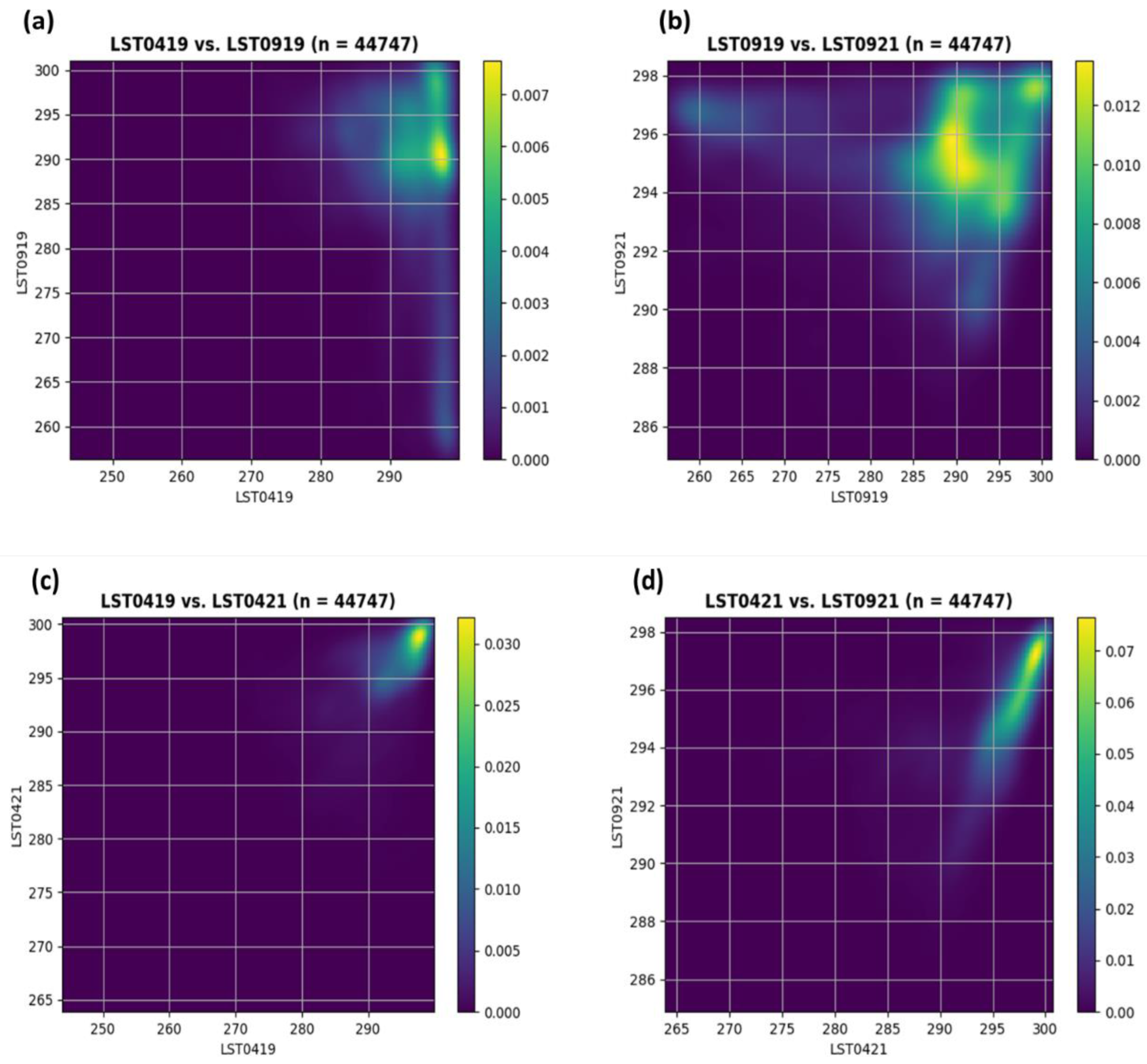
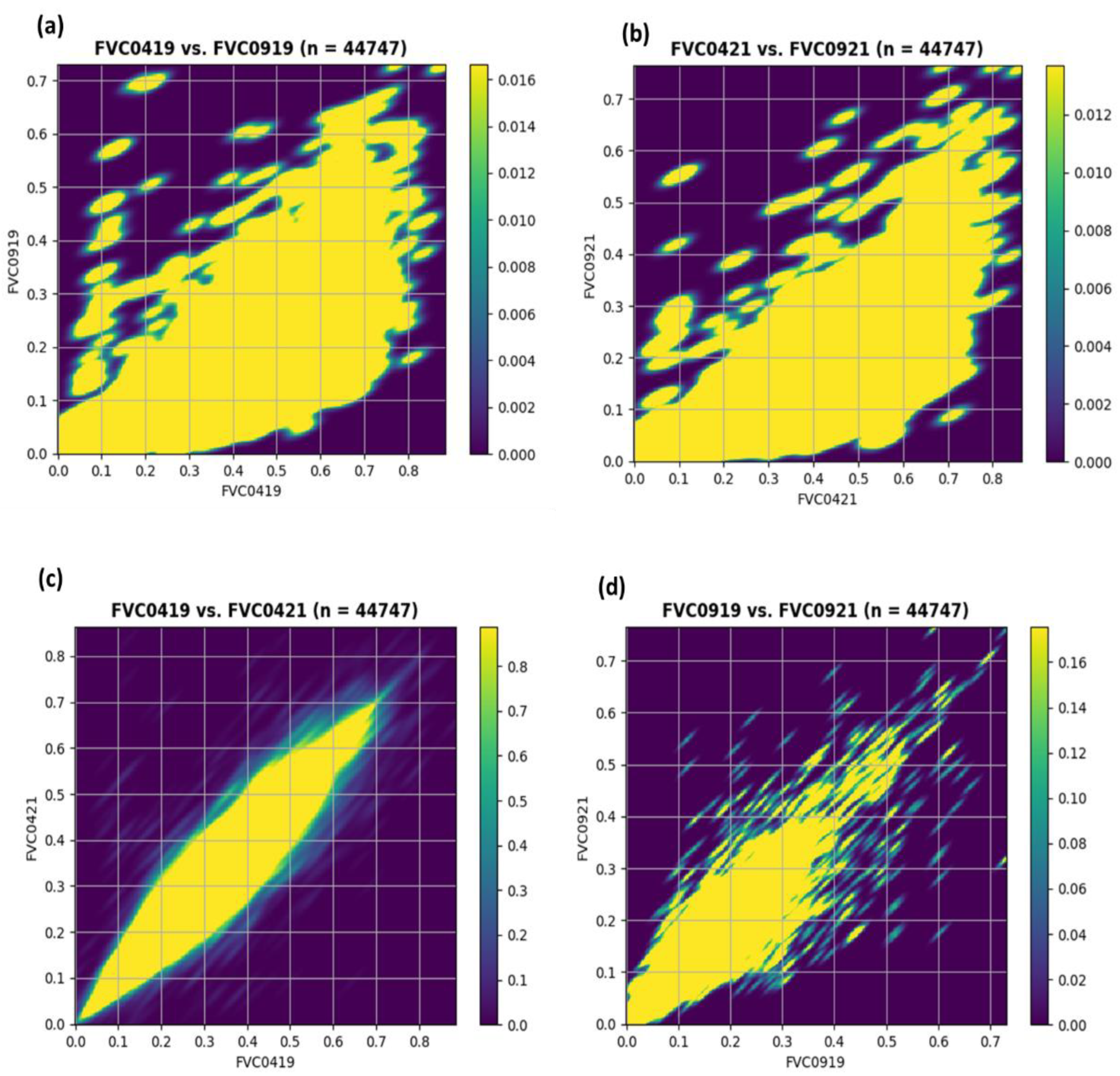
3.1.4. Correlation Analysis among Essential Climatic Variables (ECVs) under Investigation

ECVs results demonstrate a strong dual correlation of TCWV between wet and dry seasons, as presented in Figure 7a,c. This can be attributed to moisture content variation, additional synergistic modifications of the atmosphere, and variations in cloud cover since TCWV is a primary component of clouds and water vapor content. According to Halloway and Neelin [115], precipitation increases with TCWV in the tropics at different time frames, yielding a strong correlation in April. There was a significant positive correlation of TCWV between the same months in the two years, revealing that no change has occurred in this variation over time (Figure 7b,d). This implies that TCWV between the same months in the two years were influenced by the same forces and factors—for instance, an increase or decrease in precipitation and relative humidity. This corroborates with previous studies which indicated that TCWV demonstrates positive trends that are consistent with relative humidity [113,116]. Wang et al. (2016) [117] found that positive and weaker trends of TCWV are associated with the slowdown of global warming. This finding also implies that positive and stronger TCWV correlation and trends may also be attributed to accelerating global warming whose effects are adverse in arid and semiarid regions where the lower eastern region under study lies. Further, as noted by Borger et al. (2022) [116], TCWV changes correlate well with near-surface relative humidity and surface air temperature as well. This is also supported by Neelin et al. (2022) [118] who indicated that atmospheric water vapor is found within the atmospheric boundary layer and, therefore, column water vapor corelates and relates with near relative humidity as well as near surface dew point temperature.
LST demonstrates a negligible to marginally weak positive correlation in April and September 2019 (Figure 8a,b), which has a consistent pattern between September 2019 and 2021 (Figure 8d). In April 2019 and 2021, a strong positive correlation occurred, similar to April and September 2021 (Figure 8c,d). LST correlation may arise due to changes in vegetation cover between the dry and rainy seasons, vegetation and land use characteristic coverage, anthropization, and atmospheric conditions as evidenced by changes in cloud cover, which might result in uncertainties. Studies have demonstrated that land cover and land use exhibit considerably the distribution and intensity of LST [119] as well as vegetation. There exists a strong correlation between LST and vegetation where low vegetation during the dry season demonstrates high LST, and dense vegetation in the rainy season exhibits low LST [120]. Additionally, increased water vapor, which controls and determines energy amount and fluxes from the earth to the atmosphere, also affects LST variations. Further, this might be influenced by cloud cover while extracting the data.
Between April and September in both years (Figure 9a,b), a curvilinear relationship existed in FVC variation. This can be explained by the gradual and inconsistent changes in moisture content, the intensity of human agricultural activities, coupled effects between agricultural activities, and climate variability between the wet (April) and dry season (September). In addition, it is worth noting that a shift in the amount of precipitation may lead as well to the readjustment of agricultural crops in the region between wet and dry seasons, hence influencing food availability. Studies have shown that climate and human activities are key driving forces of FVC in addition to moisture index [59,121,122]. There was a strong correlation between April and September in both years (Figure 9c,d), which can be attributed to differences in moisture content between the two periods, hydrothermal characteristics, and consistency of precipitation in April and a contrary situation in September. Studies indicate that FVC can increase and decrease abruptly for a short period, and it is positively correlated with precipitation and moisture index [59,121,123].

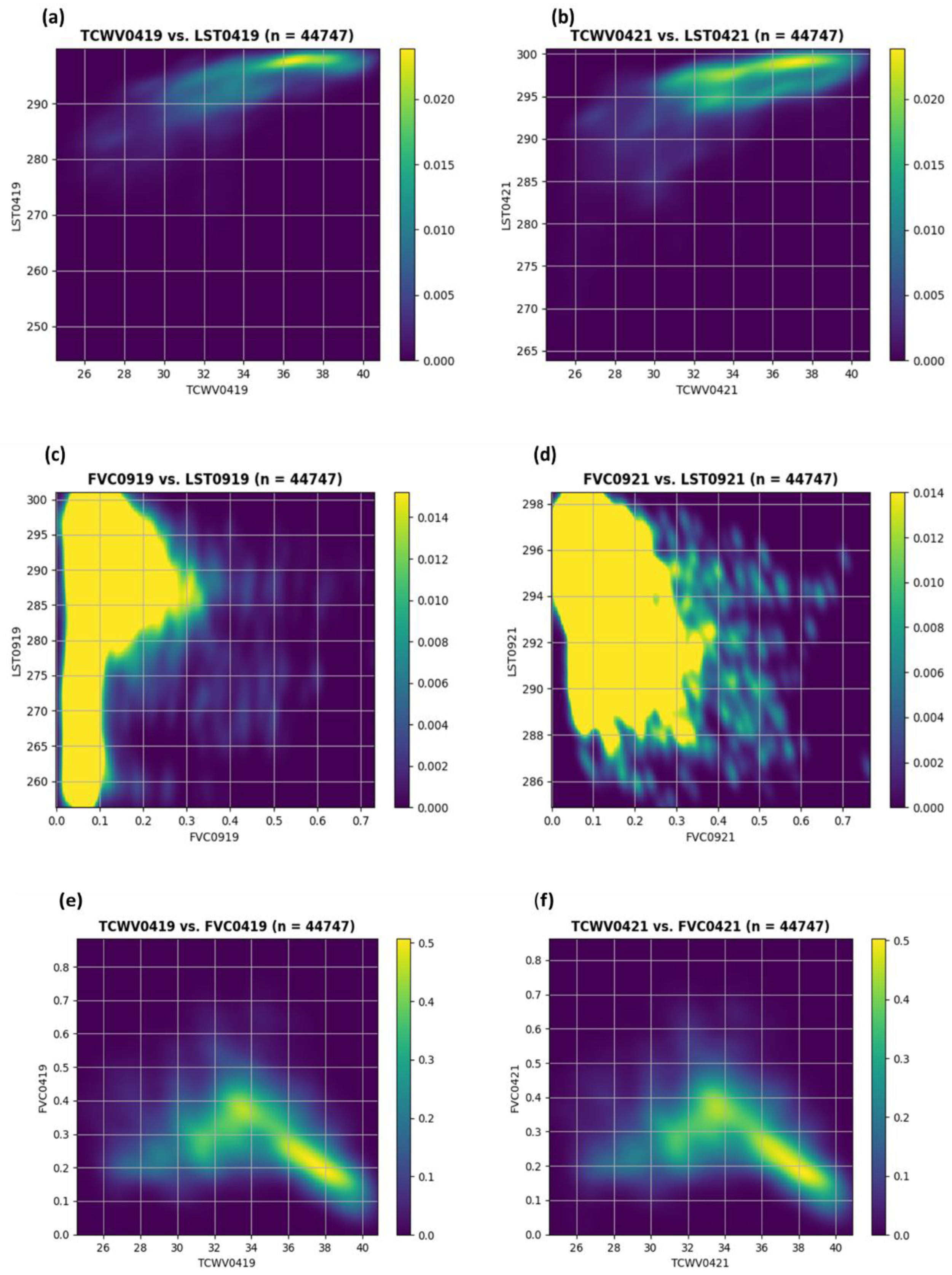
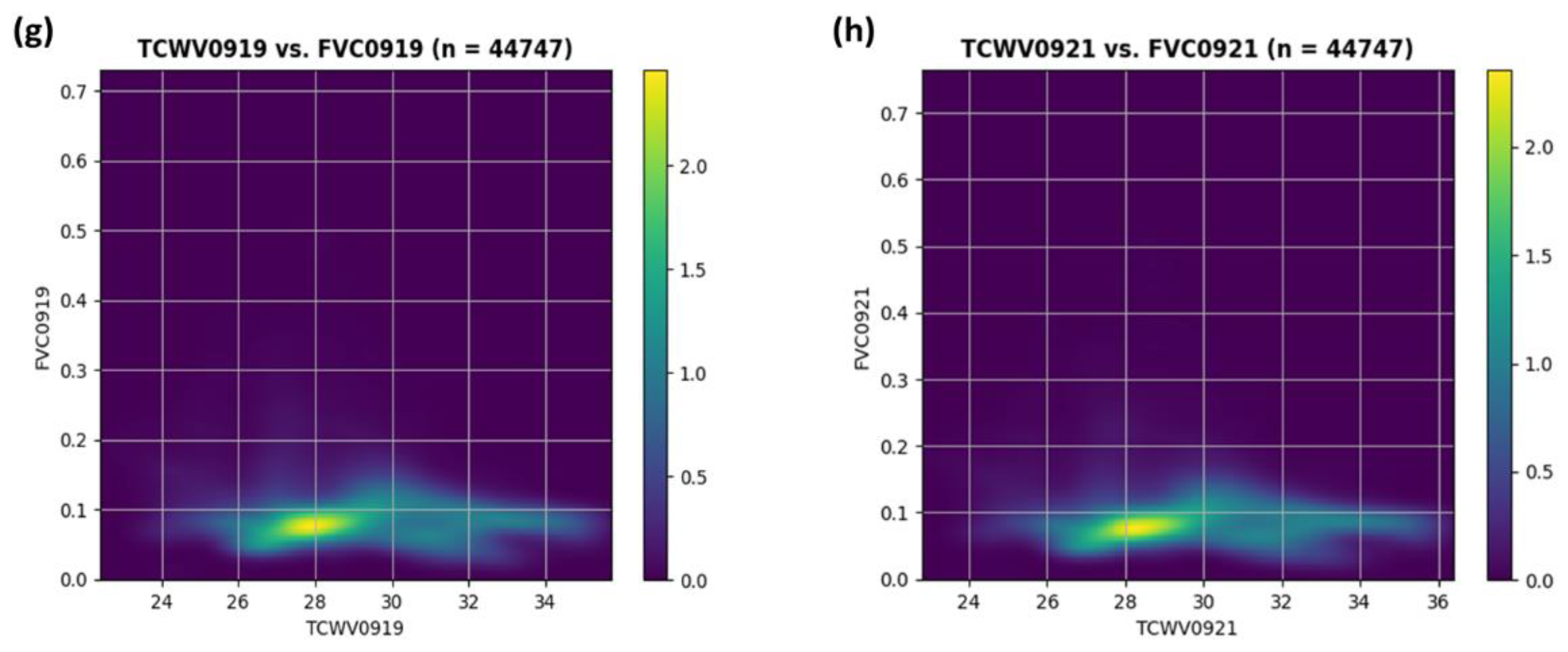
3.1.5. Density Plots for Correlation between Different Essential Climate Variables

Correlation analysis of ECVs for April and September 2019 and 2021 indicated that TCWV and LST variables displayed a moderate positive correlation between the two months and the two years, as seen in Figure 10a,b. However, Figure 10c,d demonstrate a negligible to weak negative correlation between LST and FVC. Because of the cooling effect of dense vegetation, which affects LST spatial-temporal distribution in the study area, the marginal correlation between LST and FVC was inverse, suggesting that the lower the estimated LST value is, the higher the estimated FVC value is. This may be attributed to inflection by either sparse or dense vegetation during dry and wet seasons, respectively. According to Yang et al. [124], seasonality significantly impacts FVC. For instance, in summer, the correlation with LST is expected to increase [125]. In addition, Amiri et al. [28] examined the association between land surface temperature and fractional vegetation cover and established that higher FVC corresponds to relatively lower LST values. In contrast, areas with high land surface temperatures showed a decrease in fractional vegetation cover, which is consistent with our findings of a correlation between fractional vegetation cover and land surface temperature. Similar results were found between FVC and LST during the growing season in North China [98]. Furthermore, a similar negative correlation between land surface temperature and FVC was established by [98,126] in the Island Coastal City and Fujian province in China.
Figure 10e,f revealed a double (positive and negative) correlation between TCWV and FVC in April 2019. However, some areas behaved as outliers. Moreover, Figure 10g,h showed a weak correlation between the variables in September 2021. This interpretation is confirmed by Shivers et al. [127], who found that water vapor and fractional vegetation cover do not display a robust association. This is due to low evapotranspiration rates, which typically have few or no leaves and may heighten the water vapor gradient, as well as insufficient soil moisture brought on by dry climatic conditions in September.

4. Conclusions

The results show varying patterns of the ECVs across the studied counties. For instance, land surface temperature has drastically changed over time, with Kitui and Taita Taveta counties having the highest estimates of above 20 °C in 2019. Furthermore, a significant spatial variation of TCWV was observed across the counties, with values less than 26 mm in Machakos county during the dry season of 2019, while Kitui and Taita Taveta counties had the highest estimates of greater than 36 mm during the wet season in 2021. The study also demonstrates a close relationship between ECVs and precipitation patterns as higher values were observed across the counties. During April, a wet season, FVC values were high (40–60%) across the counties, with a few exceptions where the values were high (80–100%). A varying correlation between individual (LST to LST) and different (LST to TCWV) variables between the years and seasons was clearly demonstrated by the density plots. The study demonstrates Sentinel-3 SLSTR imagery efficiency in assessing vegetation changes, land surface temperature, and total column water vapor between wet and dry seasons. Remote sensing tools provide new opportunities for investigating seasonal and annual changes in vegetation, land surface temperature, and water content, among other environmental components where subtle changes are associated with drought events occurrence. The main goals are to analyze remotely sensed data for the last three years for short-term drought detection and soil moisture loss scenarios and interpret the associated variables, which vary geographically from one geographic location to another. This paper demonstrates the potential of ECVs extracted from sentinel-3 SLSTR data for short-term drought events investigation and soil moisture fluctuation episodes in the lower eastern counties of Kenya. These findings contribute to a better understanding of short-term drought episodes and their impact on land cover dynamics. This is fundamental in enhancing our understanding of ecological changes, malfunctioning of ecosystems, ecosystems stress, and degradation of various ecosystems caused by climate change at local, regional, and global scales across arid and semi-arid environments. The study recommends climate education, awareness, and information for farmers as they prepare for the planting seasons to make informed decisions on the crops to grow in various seasons which can boost productivity for the agricultural sector and cushion people against food insecurity in the region and Kenya at large. The study is also fundamental for future climate variability preparedness in drought-prone or -risk counties, resilience planning, and policy-making more so in these regimes of climate change. Future studies will focus on comparing Sentinel-3 SLSTR products, Moderate Resolution Imaging Spectroradiometer (MODIS), Visible Infrared Imaging Radiometer Suite (VIIR), and ECOSTRESS with in situ data in drought analysis and examine other factors influencing hydrological and environmental processes and their implications under different climatic conditions.

Author Contributions

Conceptualization: P.K.M. and G.S.; methodology, G.S. and B.S.; data processing G.S.; code writing, B.S.; validation, G.S. and B.S.; formal analysis, P.K.M., G.S. and B.S.; investigation, P.K.M., G.S. and B.S.; writing—original draft preparation, P.K.M.; writing—review and editing, P.K.M., G.S., G.T., T.W. and B.S.; visualization, P.K.M., G.S., G.T., T.W. and B.S.; data interpretation, P.K.M., G.S., G.T., T.W. and B.S.; manuscript revision, G.T., T.W. and B.S. All authors have read and agreed to the published version of the manuscript.

Funding

This research received no external funding.

Data Availability Statement

The data that supported this research can be found on the Copernicus Open Access Hub (https://scihub.copernicus.eu/dhus/#/home, accessed on 11 October 2022). The python code used can be shared by the corresponding author upon request.

Acknowledgments

The authors would like to thank the editors, assistant editors, and anonymous reviewers for their valuable and constructive comments that helped enhance and improve the quality of this scientific article.

Conflicts of Interest

The authors declare no conflict of interest.

References

  1. Rossi, G. Drought Mitigation Measures: A Comprehensive Framework. In Drought and Drought Mitigation in Europe; Vogt, J.V., Somma, F., Eds.; Advances in Natural and Technological Hazards Research; Springer: Dordrecht, The Netherlands, 2000; 14p. [Google Scholar] [CrossRef]
  2. Musyimi, P.K.; Huho, J.M.; Opiyo, F.E. Understanding Drought Characteristics and Perceived Effects on Water Sources in Kenya’s Drylands: A Case Study of Makindu Sub-County. In Advancing Africa’s Sustainable Development: Proceedings of the 4th Conference on Science Advancement; Fymat, A.L., Kapalanga, J., Eds.; Cambridge Scholars Publishing: Newcastle upon Tyne, UK, 2018; pp. 324–349. ISBN 1-5275-0655-X. [Google Scholar]
  3. Payus, C.; Huey, L.A.; Adnan, F.; Rimba, A.B.; Mohan, G.; Chapagain, S.K.; Roder, G.; Gasparatos, A.; Fukushi, K. Impact of Extreme Drought Climate on Water Security in North Borneo: Case Study of Sabah. Water 2020, 12, 1135. [Google Scholar] [CrossRef] [Green Version]
  4. Tabari, H. Climate change impact on flood and extreme precipitation increases with water availability. Sci. Rep. 2020, 10, 13768. [Google Scholar] [CrossRef] [PubMed]
  5. Dai, H. Roles of Surface Albedo, Surface Temperature and Carbon Dioxide in the Seasonal Variation of Arctic Amplification. Geophys. Res. Lett. 2021, 48, e2020GL090301. [Google Scholar] [CrossRef]
  6. Wilhite, D.A.; Glantz, M.H. Understanding: The Drought Phenomenon: The Role of Definitions. Water Int. 1985, 10, 111–120. [Google Scholar] [CrossRef] [Green Version]
  7. Masson-Delmotte, V.P.; Zhai, A.; Pirani, S.L.; Connors, C.; Péan, S.; Berger, N.; Caud, Y.; Chen, L.; Goldfarb, M.I.; Gomis, M.; et al. (Eds.) Climate Change 2021: The Physical Science Basis. Contribution of Working Group I to the Sixth Assessment Report of the Intergovernmental Panel on Climate Change; Cambridge University Press: Cambridge, UK; New York, NY, USA, 2021; Available online: https://report.ipcc.ch/ar6/wg1/IPCC_AR6_WGI_FullReport.pdf (accessed on 6 December 2022).
  8. Ssenyunzi, R.C.; Oruru, B.; D’ujanga, F.M.; Realini, E.; Barindelli, S.; Tagliaferro, G.; von Engeln, A.; van de Giesen, N. Performance of ERA5 data in retrieving Precipitable Water Vapour over East African tropical region. Adv. Space Res. 2020, 65, 1877–1893. [Google Scholar] [CrossRef]
  9. Alahacoon, N.; Edirisinghe, M.; Ranagalage, M. Satellite-Based Meteorological and Agricultural Drought Monitoring for Agricultural Sustainability in Sri Lanka. Sustainability 2021, 13, 3427. [Google Scholar] [CrossRef]
  10. Varghese, D.; Radulović, M.; Stojković, S.; Crnojević, V. Reviewing the Potential of Sentinel-2 in Assessing the Drought. Remote Sens. 2021, 13, 3355. [Google Scholar] [CrossRef]
  11. Sahbeni, G. A PLSR model to predict soil salinity using Sentinel-2 MSI data. Open Geosci. 2021, 13, 977–987. [Google Scholar] [CrossRef]
  12. Zanni, S.; De Rosa, A. Remote Sensing Analyses on Sentinel-2 Images: Looking for Roman Roads in Srem Region (Serbia). Geosciences 2019, 9, 25. [Google Scholar] [CrossRef] [Green Version]
  13. Rousta, I.; Olafsson, H.; Moniruzzaman; Zhang, H.; Liou, Y.-A.; Mushore, T.D.; Gupta, A. Impacts of Drought on Vegetation Assessed by Vegetation Indices and Meteorological Factors in Afghanistan. Remote Sens. 2020, 12, 2433. [Google Scholar] [CrossRef]
  14. Sahbeni, G. Soil salinity mapping using Landsat 8 OLI data and regression modeling in the Great Hungarian Plain. SN Appl. Sci. 2021, 3, 587. [Google Scholar] [CrossRef]
  15. Borges, J.; Higginbottom, T.P.; Symeonakis, E.; Jones, M. Sentinel-1 and Sentinel-2 Data for Savannah Land Cover Mapping: Optimising the Combination of Sensors and Seasons. Remote Sens. 2020, 12, 3862. [Google Scholar] [CrossRef]
  16. Ng, W.-T.; Rima, P.; Einzmann, K.; Immitzer, M.; Atzberger, C.; Eckert, S. Assessing the Potential of Sentinel-2 and Pléiades Data for the Detection of Prosopis and Vachellia spp. in Kenya. Remote Sens. 2017, 9, 74. [Google Scholar] [CrossRef] [Green Version]
  17. Cheng, Y.; Vrieling, A.; Fava, F.; Meroni, M.; Marshall, M.; Gachoki, S. Phenology of short vegetation cycles in Kenyan rangeland from PlanetScope and Sentinel-2. Remote Sens. Environ. 2020, 248, 112004. [Google Scholar] [CrossRef]
  18. Hunt, S.E.; Mittaz, J.P.D.; Smith, D.; Polehampton, E.; Yemelyanova, R.; Woolliams, E.R.; Donlon, C. Comparison of the Sentinel-3A and B SLSTR Tandem Phase Data Using Metrological Principles. Remote Sens. 2020, 12, 2893. [Google Scholar] [CrossRef]
  19. Smith, D.; Hunt, S.E.; Etxaluze, M.; Peters, D.; Nightingale, T.; Mittaz, J.; Woolliams, E.R.; Polehampton, E. Traceability of the Sentinel-3 SLSTR Level-1 Infrared Radiometric Processing. Remote Sens. 2021, 13, 374. [Google Scholar] [CrossRef]
  20. Jonas, F.; Martin, K.; Daniel, W. Quantifying forest cover at Mount Kenya: Use of Sentinel-2 for a discrimination of tropical tree composites. Afr. J. Environ. Sci. Technol. 2020, 14, 159–176. [Google Scholar] [CrossRef]
  21. Ghulam, A.; Qin, Q.; Teyip, T.; Li, Z.-L. Modified perpendicular drought index (MPDI): A real-time drought monitoring method. ISPRS J. Photogramm. Remote Sens. 2007, 62, 150–164. [Google Scholar] [CrossRef]
  22. Jing, X.; Yao, W.-Q.; Wang, J.-H.; Song, X.-Y. A study on the relationship between dynamic change of vegetation coverage and precipitation in Beijing’s mountainous areas during the last 20 years. Math. Comput. Model. 2011, 54, 1079–1085. [Google Scholar] [CrossRef]
  23. Duveiller, G.; Lopez-Lozano, R.; Cescatti, A. Exploiting the multi-angularity of the MODIS temporal signal to identify spatially homogeneous vegetation cover: A demonstration for agricultural monitoring applications. Remote Sens. Environ. 2015, 166, 61–77. [Google Scholar] [CrossRef]
  24. Yang, R.; Yu-Lin, D.; Mao, D.; Wang, Z.; Tian, Y.; Dong, Y. Examining Fractional Vegetation Cover Dynamics in Response to Climate from 1982 to 2015 in the Amur River Basin for SDG 13. Sustainability 2020, 12, 5866. [Google Scholar] [CrossRef]
  25. Mu, B.; Zhao, X.; Zhao, J.; Liu, N.; Si, L.; Wang, Q.; Sun, N.; Sun, M.; Guo, Y.; Zhao, S. Quantitatively Assessing the Impact of Driving Factors on Vegetation in China’s 32 Major Cities. Remote Sens. 2022, 14, 839. [Google Scholar] [CrossRef]
  26. Kalnay, E.; Cai, M. Impact of urbanization and land-use change on climate. Nature 2003, 423, 528–531. [Google Scholar] [CrossRef]
  27. Cheng, K.-S.; Su, Y.-F.; Kuo, F.-T.; Hung, W.-C.; Chiang, J.-L. Assessing the effect of landcover changes on air temperature using remote sensing images—A pilot study in northern Taiwan. Landsc. Urban Plan. 2008, 85, 85–96. [Google Scholar] [CrossRef]
  28. Amiri, R.; Weng, Q.; Alimohammadi, A.; Alavipanah, S.K. Spatial–temporal dynamics of land surface temperature in relation to fractional vegetation cover and land use/cover in the Tabriz urban area, Iran. Remote Sens. Environ. 2009, 113, 2606–2617. [Google Scholar] [CrossRef]
  29. Lai, Y.-J.; Li, C.-F.; Lin, P.-H.; Wey, T.-H.; Chang, C.-S. Comparison of MODIS land surface temperature and ground-based observed air temperature in complex topography. Int. J. Remote Sens. 2012, 33, 7685–7702. [Google Scholar] [CrossRef]
  30. Zhang, D.; Tang, R.; Zhao, W.; Tang, B.; Wu, H.; Shao, K.; Li, Z.-L. Surface Soil Water Content Estimation from Thermal Remote Sensing based on the Temporal Variation of Land Surface Temperature. Remote Sens. 2014, 6, 3170–3187. [Google Scholar] [CrossRef] [Green Version]
  31. Harris, P.P.; Folwell, S.S.; Gallego-Elvira, B.; Rodríguez, J.; Milton, S.; Taylor, C.M. An Evaluation of Modeled Evaporation Regimes in Europe Using Observed Dry Spell Land Surface Temperature. J. Hydrometeorol. 2017, 18, 1453–1470. [Google Scholar] [CrossRef] [Green Version]
  32. Metz, M.; Andreo, V.; Neteler, M. A New Fully Gap-Free Time Series of Land Surface Temperature from MODIS LST Data. Remote Sens. 2017, 9, 1333. [Google Scholar] [CrossRef] [Green Version]
  33. Mustafa, E.K.; El-Hamid, H.T.A.; Tarawally, M. Spatial and temporal monitoring of drought based on land surface temperature, Freetown City, Sierra Leone, West Africa. Arab. J. Geosci. 2021, 14, 1013. [Google Scholar] [CrossRef]
  34. Mustafa, E.K.; Liu, G.; El-Hamid, H.T.A.; Kaloop, M.R. Simulation of land use dynamics and impact on land surface temperature using satellite data. GeoJournal 2021, 86, 1089–1107. [Google Scholar] [CrossRef]
  35. Grossi, M.; Valks, P.; Loyola, D.; Aberle, B.; Slijkhuis, S.; Wagner, T.; Beirle, S.; Lang, R. Total column water vapour measurements from GOME-2 MetOp-A and MetOp-B. Atmos. Meas. Tech. 2015, 8, 1111–1133. [Google Scholar] [CrossRef] [Green Version]
  36. Namaoui, H.; Kahlouche, S.; Belbachir, A.H.; Van Malderen, R.; Brenot, H.; Pottiaux, E. GPS water vapor and its comparison with radiosonde and ERA-Interim data in Algeria. Adv. Atmos. Sci. 2017, 34, 623–634. [Google Scholar] [CrossRef]
  37. Lindstrot, R.; Stengel, M.; Schröder, M.; Fischer, J.; Preusker, R.; Schneider, N.; Steenbergen, T.; Bojkov, B.R. A global climatology of total columnar water vapour from SSM/I and MERIS. Earth Syst. Sci. Data 2014, 6, 221–233. [Google Scholar] [CrossRef] [Green Version]
  38. GoK. Republic of Kenya. Economic Survey, 2013. Kenya National Bureau of Statistics (KNBS), Nairobi, Kenya. 2013. Available online: https://academia-ke.org/library/download/knbs-kenya-economic-survey-2013-january-2014/?wpdmdl=7734&refresh=62053100c470c1644507392 (accessed on 7 November 2022).
  39. Wanyama, D.; Moore, N.J.; Dahlin, K.M. Persistent Vegetation Greening and Browning Trends Related to Natural and Human Activities in the Mount Elgon Ecosystem. Remote Sens. 2020, 12, 2113. [Google Scholar] [CrossRef]
  40. Muema, E.; Mburu, J.; Coulibaly, J.; Mutune, J. Determinants of access and utilisation of seasonal climate information services among smallholder farmers in Makueni County, Kenya. Heliyon 2018, 4, e00889. [Google Scholar] [CrossRef] [Green Version]
  41. GoK. Kenya Population and Housing Census Volume I: Population by County and Sub-County. Government Printer. 2019. Available online: https://www.knbs.or.ke/?wpdmpro=2019-kenya-population-and-housing-census-volume-i-population-by-county-and-sub-county (accessed on 7 November 2022).
  42. Akuja, T.E.; Kandagor, J. A review of policies and agricultural productivity in the arid and semi-arid lands (ASALS), Kenya: The case of Turkana County. J. Appl. Biosci. 2019, 140, 14304. [Google Scholar] [CrossRef]
  43. CCKP (Climate Change Knowledge Portal). Kenya Projected Future Climate. URL. 2020. Available online: https://climateknowledgeportal.worldbank.org/country/Kenya/climate-data-projections (accessed on 10 October 2022).
  44. Marshall, M.T.; Funk, C.; Michaelsen, J. Agricultural Drought Monitoring in Kenya Using Evapotranspiration Derived from Remote Sensing and Reanalysis Data. In Remote Sensing of Drought: Innovative Monitoring Approaches; Wardlow, B.D., Anderson, M.C., Verdin, J.P., Eds.; CRC Press/Taylor & Francis: Boca Raton, FL, USA, 2012; pp. 169–193. Available online: http://digitalcommons.unl.edu/usgsstaffpub/978 (accessed on 1 September 2022).
  45. Huho, J.M.; Mashara, J.N.; Musyimi, P.K. Profiling Disasters in Kenya and their causes. Acad. Res. Int. J. 2016, 7, 290–305. Available online: http://www.savap.org.pk/journals/ARInt./Vol.7(1)/2016(7.1-30).pdf (accessed on 10 November 2022).
  46. Downing, T.; Watkiss, P.; Dyszynski, J.; Butterfield, R.; Devisscher, T.; Pye, S.; Sang, J. The Economics of Climate Change in Kenya: Final Report Submitted in Advance of COP15. 2009. Available online: https://mediamanager.sei.org/documents/Publications/SEI-ProjectReport-Downing-EconomicsOfClimateChangeKenya-2009.pdf (accessed on 2 February 2023).
  47. Ajuang, C.O.; Abuom, P.O.; Bosire, E.K.; Dida, G.O.; Anyona, D.N. Determinants of climate change awareness level in upper Nyakach Division, Kisumu County, Kenya. Springer Plus 2016, 5, 1015. [Google Scholar] [CrossRef] [Green Version]
  48. Huho, J.M. An Analysis of Rainfall Characteristics in Machakos County, Kenya. IOSR J. Environ. Sci. Toxicol. Food Technol. 2017, 11, 64–72. [Google Scholar] [CrossRef]
  49. Maguta, J.K.; Nzengya, D.M.; Mutisya, C.; Wairimu, J. Building Capacity to Cope with Climate change-induced Resource-Based Conflicts among Grassroots Communities in Kenya. In African Handbook of Climate Change Adaptation; Leal Filho, W., Oguge, N., Ayal, D., Adeleke, L., da Silva, I., Eds.; Springer: Cham, Swizerland, 2021; pp. 2611–2630. [Google Scholar] [CrossRef]
  50. Indiatsy, C.M. Analysis of Historical Monthly, Seasonal and Annual Rainfall Variability (1990–2014) in Machakos Sub County, Kenya. Int. J. Multidiscip. Curr. Res. 2018, 6, 21–41. [Google Scholar] [CrossRef] [Green Version]
  51. Musyimi, P.K.; Huho, J.M.; Nduru, G.M.; Opiyo, F.E. Assessment of Suitability of Adaptation Strategies to Water Scarcity in Makindu Sub-County, Kenya. Acad. Res. Int. 2017, 8, 115–123. Available online: http://www.savap.org.pk/journals/ARInt./Vol.8(2)/ARInt.2017(8.2-11).pdf (accessed on 10 September 2022).
  52. Khisa, G.V. Peoples’ perception on climate change and its effects on livelihood in Kitui County. Int. J. Sustain. Dev. Plan. 2018, 7, 70–81. Available online: https://isdsnet.com/ijds-v7n1-05.pdf (accessed on 10 November 2022).
  53. Mutunga, E.J.; Ndungu, C.K.; Muendo, P. Smallholder Farmers’ Perceptions and Adaptations to Climate Change and Variability in Kitui County, Kenya. J. Earth Sci. Clim. Chang. 2017, 8, 389. [Google Scholar]
  54. Mwangi, M.; Kituyi, E.; Ouma, G.; Macharia, D. Indicator Approach to Assessing Climate Change Vulnerability of Communities in Kenya: A Case Study of Kitui County. Am. J. Clim. Chang. 2020, 9, 53–67. [Google Scholar] [CrossRef] [Green Version]
  55. Ogallo, L.; Omay, P.; Kabaka, G.; Lutta, I. Report on Historical Climate Baseline Statistics for Taita Taveta, Kenya Vol. 1; IGAD Climate Prediction and Application Centre: Ngong, Kenya, 2019. [Google Scholar] [CrossRef]
  56. Autio, A.; Johansson, T.; Motaroki, L.; Minoia, P.; Pellikka, P. Constraints for adopting climate-smart agricultural practices among smallholder farmers in Southeast Kenya. Agric. Syst. 2021, 194, 103284. [Google Scholar] [CrossRef]
  57. ESA. Sentinel-3 SLSTR User Guide. 2022. Available online: https://sentinel.esa.int/web/sentinel/user-guides/sentinel-3-slstr (accessed on 1 September 2022).
  58. Coppo, P.; Ricciarelli, B.; Brandani, F.; Delderfield, J.; Ferlet, M.; Mutlow, C.; Munro, G.; Nightingale, T.; Smith, D.; Bianchi, S.; et al. SLSTR: A high accuracy dual scan temperature radiometer for sea and land surface monitoring from space. J. Mod. Opt. 2010, 57, 1815–1830. [Google Scholar] [CrossRef]
  59. Yang, J.; Zhou, J.; Göttsche, F.-M.; Long, Z.; Ma, J.; Luo, R. Investigation and validation of algorithms for estimating land surface temperature from Sentinel-3 SLSTR data. Int. J. Appl. Earth Obs. Geoinf. 2021, 91, 102136. [Google Scholar] [CrossRef]
  60. Wooster, M.; Xu, W.; Nightingale, T. Sentinel-3 SLSTR active fire detection and FRP product: Pre-launch algorithm development and performance evaluation using MODIS and ASTER datasets. Remote Sens. Environ. 2012, 120, 236–254. [Google Scholar] [CrossRef]
  61. King, J.A.; Washington, R.; Engelstaedter, S. Representation of the Indian Ocean Walker circulation in climate models and links to Kenyan rainfall. Int. J. Clim. 2020, 41, E616–E643. [Google Scholar] [CrossRef]
  62. Kustas, W.; Anderson, M. Advances in thermal infrared remote sensing for land surface modeling. Agric. For. Meteorol. 2009, 149, 2071–2081. [Google Scholar] [CrossRef]
  63. Li, Z.-L.; Tang, B.-H.; Wu, H.; Ren, H.; Yan, G.; Wan, Z.; Trigo, I.F.; Sobrino, J.A. Satellite-derived land surface temperature: Current status and perspectives. Remote Sens. Environ. 2013, 131, 14–37. [Google Scholar] [CrossRef] [Green Version]
  64. ESA. User Guides: Sentinel-3 SLSTR. 2021. Available online: https://sentinels.copernicus.eu/web/sentinel/user-guides/sentinel-3-slstr/overview/geophysical-measurements/land-surface-temperature (accessed on 1 September 2022).
  65. Meng, X.; Cheng, J.; Liang, S. Estimating Land Surface Temperature from Feng Yun-3C/MERSI Data Using a New Land Surface Emissivity Scheme. Remote Sens. 2017, 9, 1247. [Google Scholar] [CrossRef] [Green Version]
  66. Solanky, V.; Singh, S.; Katiyar, S.K. Land Surface Temperature Estimation Using Remote Sensing Data. In Hydrologic Modeling. Water Science and Technology Library, 81; Singh, V., Yadav, S., Yadava, R., Eds.; Springer: Singapore, 2018. [Google Scholar] [CrossRef]
  67. Dar, I.; Qadir, J.; Shukla, A. Estimation of LST from multi-sensor thermal remote sensing data and evaluating the influence of sensor characteristics. Ann. GIS 2019, 25, 263–281. [Google Scholar] [CrossRef] [Green Version]
  68. Vlassova, L.; Perez-Cabello, F.; Nieto, H.; Martín, P.; Riaño, D.; De La Riva, J. Assessment of Methods for Land Surface Temperature Retrieval from Landsat-5 TM Images Applicable to Multiscale Tree-Grass Ecosystem Modeling. Remote Sens. 2014, 6, 4345–4368. [Google Scholar] [CrossRef] [Green Version]
  69. Carlson, T.N.; Ripley, D.A. On the relation between NDVI, fractional vegetation cover, and leaf area index. Remote Sens. Environ. 1997, 62, 241–252. [Google Scholar] [CrossRef]
  70. Gao, L.; Wang, X.; Johnson, B.A.; Tian, Q.; Wang, Y.; Verrelst, J.; Mu, X.; Gu, X. Remote sensing algorithms for estimation of fractional vegetation cover using pure vegetation index values: A review. ISPRS J. Photogramm. Remote Sens. 2020, 159, 364–377. [Google Scholar] [CrossRef]
  71. Lawley, E.F.; Lewis, M.M.; Ostendorf, B. Evaluating MODIS soil fractional cover for arid regions, using albedo from high-spatial resolution satellite imagery. Int. J. Remote Sens. 2014, 35, 2028–2046. [Google Scholar] [CrossRef] [Green Version]
  72. Sun, Y.; Ren, H.; Zhou, G.; Zhang, T.; Zhang, C.Y.; Qin, Q. The estimation and validation of fractional vegetation cover based on GaoFen-4 satellite imagery. In Proceedings of the 2017 IEEE International Geoscience and Remote Sensing Symposium (IGARSS), Fort Worth, TX, USA, 23–28 July 2017; pp. 3495–3498. [Google Scholar] [CrossRef]
  73. Rouse, J.W.; Haas, R.H.; Schell, J.A.; Deering, D.W. Monitoring vegetation systems in the Great Plains with ERTS, In Third Earth Resources Technology Satellite–1 Syposium. Volume I: Technical Presentations; Freden, S.C., Mercanti, E.P., Becker, M., Eds.; NASA SP-351; NASA: Washington, DC, USA, 1974; pp. 309–317. [Google Scholar]
  74. Qi, J.; Marsett, R.; Moran, M.; Goodrich, D.; Heilman, P.; Kerr, Y.; Dedieu, G.; Chehbouni, A.; Zhang, X. Spatial and temporal dynamics of vegetation in the San Pedro River basin area. Agric. For. Meteorol. 2000, 105, 55–68. [Google Scholar] [CrossRef] [Green Version]
  75. Wu, C.; Murray, A.T. Estimating impervious surface distribution by spectral mixture analysis. Remote Sens. Environ. 2003, 84, 493–505. [Google Scholar] [CrossRef]
  76. Gutman, G.; Ignatov, A. The derivation of the green vegetation fraction from NOAA/AVHRR data for use in numerical weather prediction models. Int. J. Remote Sens. 1998, 19, 1533–1543. [Google Scholar] [CrossRef]
  77. Jiménez-Muñoz, J.C.; Sobrino, J.A.; Plaza, A.; Guanter, L.; Moreno, J.; Martínez, P. Comparison between fractional vegetation cover retrievals from vegetation indices and spectral mixture analysis: Case study of PROBA/CHRIS data over an agricultural area. Sensors 2009, 9, 768–793. [Google Scholar] [CrossRef] [PubMed] [Green Version]
  78. Chahine, M.T. The hydrological cycle and its influence on climate. Nature 1992, 359, 373–380. [Google Scholar] [CrossRef]
  79. Lacis, A.A.; Schmidt, G.A.; Rind, D.; Ruedy, R.A. Atmospheric CO2: Principal Control Knob Governing Earth’s Temperature. Science 2010, 330, 356–359. [Google Scholar] [CrossRef] [Green Version]
  80. Zhao, Y.; Zhou, T. Asian water tower evinced in total column water vapor: A comparison among multiple satellite and reanalysis data sets. Clim. Dyn. 2020, 54, 231–245. [Google Scholar] [CrossRef] [Green Version]
  81. Abbasi, B.; Qin, Z.; Du, W.; Fan, J.; Zhao, C.; Hang, Q.; Zhao, S.; Li, S. An Algorithm to Retrieve Total Precipitable Water Vapor in the Atmosphere from FengYun 3D Medium Resolution Spectral Imager 2 (FY-3D MERSI-2) Data. Remote Sens. 2020, 12, 3469. [Google Scholar] [CrossRef]
  82. Wypych, A.; Bochenek, B.; Różycki, M. Atmospheric Moisture Content over Europe and the Northern Atlantic. Atmosphere 2018, 9, 18. [Google Scholar] [CrossRef] [Green Version]
  83. Banimahd, S.; Zand-Parsa, S. Simulation of evaporation, coupled liquid water, water vapor and heat transport through the soil medium. Agric. Water Manag. 2013, 130, 168–177. [Google Scholar] [CrossRef]
  84. EUMeTrain. Product Tutorial on TPW Content Products. 2014. Available online: http://www.eumetrain.org/data/3/359/navmenu.php?tab=2&page=1.0.0 (accessed on 20 November 2022).
  85. Kitui County Integrated Development Plan (CIDP), 2018–2022: Kitui County Integrated Development Plan. 2018. Available online: https://repository.kippra.or.ke/handle/123456789/587 (accessed on 1 September 2022).
  86. Guha, S.; Govil, H.; Besoya, M. An investigation on seasonal variability between LST and NDWI in an urban environment using Landsat satellite data. Geomat. Nat. Hazards Risk 2020, 11, 1319–1345. [Google Scholar] [CrossRef]
  87. Mwangi, P.W.; Karanja, F.N.; Kamau, P.K. Analysis of the Relationship between Land Surface Temperature and Vegetation and Built-Up Indices in Upper-Hill, Nairobi. J. Geosci. Environ. Prot. 2018, 6, 1–16. [Google Scholar] [CrossRef] [Green Version]
  88. Panda, S.K.; Choudhury, S.; Saraf, A.K.; Das, J.D. MODIS land surface temperature data detects thermal anomaly preceding 8 October 2005 Kashmir earthquake. Int. J. Remote Sens. 2007, 28, 4587–4596. [Google Scholar] [CrossRef]
  89. Vancutsem, C.; Ceccato, P.; Dinku, T.; Connor, S.J. Evaluation of MODIS land surface temperature data to estimate air temperature in different ecosystems over Africa. Remote Sens. Environ. 2010, 114, 449–465. [Google Scholar] [CrossRef]
  90. Amantai, N.; Ding, J. Analysis on the Spatio-Temporal Changes of LST and Its Influencing Factors Based on VIC Model in the Arid Region from 1960 to 2017: An Example of the Ebinur Lake Watershed, Xinjiang, China. Remote Sens. 2021, 13, 4867. [Google Scholar] [CrossRef]
  91. Ahmed, B.; Kamruzzaman, M.; Zhu, X.; Rahman, M.S.; Choi, K. Simulating Land Cover Changes and Their Impacts on Land Surface Temperature in Dhaka, Bangladesh. Remote Sens. 2013, 5, 5969–5998. [Google Scholar] [CrossRef] [Green Version]
  92. Kok, J.F.; Ward, D.S.; Mahowald, N.M.; Evan, A.T. Global and regional importance of the direct dust-climate feedback. Nat. Commun. 2018, 9, 241. [Google Scholar] [CrossRef] [PubMed] [Green Version]
  93. Cui, Y.Y.; de Foy, B. Seasonal Variations of the Urban Heat Island at the Surface and the Near-Surface and Reductions due to Urban Vegetation in Mexico City. J. Appl. Meteorol. Clim. 2012, 51, 855–868. [Google Scholar] [CrossRef]
  94. Li, R.; Wang, C.; Wu, D. Changes in precipitation recycling over arid regions in the Northern Hemisphere. Theor. Appl. Clim. 2018, 131, 489–502. [Google Scholar] [CrossRef] [Green Version]
  95. Faramarzi, M.; Heidarizadi, Z.; Mohamadi, A.; Heydari, M. Detection of vegetation changes in relation to normalized difference vegetation index (NDVI) in semi-arid rangeland in western Iran. J. Agric. Sci. Technol. 2018, 20, 51–60. Available online: https://jast.modares.ac.ir/article-23-10153-en.pdf (accessed on 10 October 2022).
  96. Yang, T.; Ala, M.; Zhang, Y.; Wu, J.; Wang, A.; Guan, D. Characteristics of soil moisture under different vegetation coverage in Horqin Sandy Land, northern China. PLoS ONE 2018, 13, e0198805. [Google Scholar] [CrossRef] [PubMed]
  97. Ji, F.; Wu, Z.; Huang, J.; Chassignet, E.P. Evolution of land surface air temperature trend. Nat. Clim. Chang. 2014, 4, 462–466. [Google Scholar] [CrossRef]
  98. Qiao, R.; Dong, C.; Ji, S.; Chang, X. Spatial Scale Effects of the Relationship between Fractional Vegetation Coverage and Land Surface Temperature in Horqin Sandy Land, North China. Sensors 2021, 21, 6914. [Google Scholar] [CrossRef] [PubMed]
  99. Rahimzadeh-Bajgiran, P.; Omasa, K.; Shimizu, Y. Comparative Evaluation of the Vegetation Dryness Index (VDI), the Temperature Vegetation Dryness Index (TVDI) and the Improved TVDI (iTVDI) for Water Stress Detection in Semi-Arid Regions of Iran. ISPRS-J. Photogramm. Remote Sens. 2012, 68, 1–12. [Google Scholar] [CrossRef]
  100. Holzman, M.E.; Rivas, R.; Piccolo, M.C. Estimating Soil Moisture and the Relationship with Crop Yield Using Surface Temperature and Vegetation Index. Int. J. Appl. Earth Obs. Geoinf. 2014, 28, 181–192. [Google Scholar] [CrossRef]
  101. Areffian, A.; Eslamian, S.; Sadr, M.K.; Khoshfetrat, A. Monitoring the Effects of Drought on Vegetation Cover and Ground Water Using MODIS Satellite Images and ANN. KSCE J. Civ. Eng. 2021, 25, 1095–1105. [Google Scholar] [CrossRef]
  102. EUMETSAT. Available online: https://navigator.eumetsat.int/product/EO:EUM:DAT:MSG:FVC-SEVIRI/print.2017 (accessed on 29 May 2023).
  103. Musau, M.; Mugo, J. Anthropogenic influences on species composition and diversity dryland forest fragments Kitui, Eastern Kenya. East Afr. Agric. For. J. 2021, 84, 181–194. Available online: https://www.kalro.org/www.eaafj.or.ke/index.php/path/issue/view/44 (accessed on 7 December 2022).
  104. UNEP. Global Environment Outlook. Environment for Development. Nairobi, Kenya, 2007. Available online: https://wedocs.unep.org/handle/20.500.11822/7646;jsessionid=166F1A4FA202BB68319E13938C492226 (accessed on 7 December 2022).
  105. Archibald, S.; Scholes, R.J. Leaf green-up in a semi-arid African savanna separating tree and grass responses to environmental cues. J. Veg. Sci. 2007, 18, 583–594. Available online: http://www.jstor.org/stable/4499264 (accessed on 10 January 2023).
  106. Guo, B.; Zhang, J.; Meng, X.; Xu, T.; Song, Y. Long-term spatio-temporal precipitation variations in China with precipitation surface interpolated by ANUSPLIN. Sci. Rep. 2020, 10, 1–17. [Google Scholar] [CrossRef] [Green Version]
  107. Nguyen, T.T. Fractional Vegetation Cover Change Detection In Megacities Using Landsat Time-Series Images: A Case Study Of Hanoi City (Vietnam) During 1986–2019. Geogr. Environ. Sustain. 2019, 12, 175–187. [Google Scholar] [CrossRef]
  108. Zhang, S.; Chen, H.; Fu, Y.; Niu, H.; Yang, Y.; Zhang, B. Fractional Vegetation Cover Estimation of Different Vegetation Types in the Qaidam Basin. Sustainability 2019, 11, 864. [Google Scholar] [CrossRef] [Green Version]
  109. Xie, L.; Meng, X.; Zhao, X.; Fu, L.; Sharma, R.P.; Sun, H. Estimating Fractional Vegetation Cover Changes in Desert Regions Using RGB Data. Remote Sens. 2022, 14, 3833. [Google Scholar] [CrossRef]
  110. Sahbeni, G.; Pleynet, J.B.; Jarocki, K. A spatiotemporal analysis of precipitation anomalies using rainfall Gini index between 1980 and 2022. Atmos. Sci. Lett. 2023, 24, e1161. [Google Scholar] [CrossRef]
  111. Taylor, C.; Lambin, E.F.; Stephenne, N.; Harding, R.J.; Essery, R. The Influence of Land Use Change on Climate in the Sahel. J. Clim. 2002, 15, 3615–3629. [Google Scholar] [CrossRef]
  112. Duguay-Tetzlaff, A.; Bento, V.A.; Göttsche, F.M.; Stöckli, R.; Martins, J.P.A.; Trigo, I.; Olesen, F.; Bojanowski, J.S.; Da Camara, C.; Kunz, H. Meteosat Land Surface Temperature Climate Data Record: Achievable Accuracy and Potential Uncertainties. Remote Sens. 2015, 7, 13139–13156. [Google Scholar] [CrossRef] [Green Version]
  113. Trenberth, K.E.; Caron, J.M. The Southern Oscillation Revisited: Sea Level Pressures, Surface Temperatures, and Precipitation. J. Clim. 2000, 13, 4358–4365. [Google Scholar] [CrossRef]
  114. Trenberth, K.E. Changes in precipitation with climate change, Contribution to CR Special 25’ Climate services for sustainable development. Clim. Res. 2011, 47, 123–138. [Google Scholar] [CrossRef] [Green Version]
  115. Holloway, C.; Neelin, J.D. Temporal Relations of Column Water Vapor and Tropical Precipitation. J. Atmos. Sci. 2010, 67, 1091–1105. [Google Scholar] [CrossRef]
  116. Borger, C.; Beirle, S.; Wagner, T. Analysis of global trends of total column water vapour from multiple years of OMI observations. Atmos. Chem. Phys. 2022, 22, 10603–10621. [Google Scholar] [CrossRef]
  117. Wang, J.; Dai, A.; Mears, C. Global Water Vapor Trend from 1988 to 2011 and Its Diurnal Asymmetry Based on GPS, Radiosonde, and Microwave Satellite Measurements. J. Climate 2016, 29, 5205–5222. [Google Scholar] [CrossRef]
  118. Neelin, J.D.; Martinez-Villalobos, C.; Stechmann, S.N.; Ahmed, F.; Chen, G.; Norris, J.M.; Kuo, Y.-H.; Lenderink, G. Precipitation Extremes and Water Vapor. Curr. Clim. Chang. Rep. 2022, 8, 17–33. [Google Scholar] [CrossRef]
  119. Gomes, Y.B.; Caracristi, I. Seasonal analysis on land surface temperature (LST) and normalized difference vegetation index (NDVI) variations in the Iguatu semi-arid hinterland, ceará. Int. J. Hydrol. 2021, 5, 289–294. [Google Scholar] [CrossRef]
  120. Marajh, L.; He, Y. Temperature Variation and Climate Resilience Action within a Changing Landscape. Remote Sens. 2022, 14, 701. [Google Scholar] [CrossRef]
  121. Mao, P.; Zhang, J.; Li, M.; Liu, Y.; Wang, X.; Yan, R.; Shen, B.; Zhang, X.; Shen, J.; Zhu, X.; et al. Spatial and temporal variations in fractional vegetation cover and its driving factors in the Hulun Lake region. Ecol. Indic. 2022, 135, 108490. [Google Scholar] [CrossRef]
  122. Xin, Z.B.; Xu, J.X.; Zheng, W. Spatiotemporal variations of vegetation cover on the Chinese Loess Plateau (1981–2006): Impacts of climate changes and human activities. Sci. China Ser. D Earth Sci. 2008, 51, 67–78. [Google Scholar] [CrossRef]
  123. Küçük, Ç.; Koirala, S.; Carvalhais, N.; Miralles, D.G.; Reichstein, M.; Jung, M. Characterizing the Response of Vegetation Cover to Water Limitation in Africa Using Geostationary Satellites. J. Adv. Model. Earth Syst. 2022, 14, e2021MS002730. [Google Scholar] [CrossRef] [PubMed]
  124. Yang, G.; Pu, R.; Zhang, J.; Zhao, C.; Feng, H.; Wang, J. Remote sensing of seasonal variability of fractional vegetation cover and its object-based spatial pattern analysis over mountain areas. ISPRS J. Photogramm. Remote Sens. 2013, 77, 79–93. [Google Scholar] [CrossRef]
  125. Li, M.; Zhong, S.; Luo, Y.; Liu, Q.; Li, X. A Study of the Change in Surface Parameters during the Last Four Decades in the MuUs Desert Based on Remote Sensing Data. Remote Sens. 2022, 14, 4025. [Google Scholar] [CrossRef]
  126. Li, Y.L.; Wang, X.Q.; Chen, Y.Z.; Wang, M.M. The correlation analysis of land surface temperature and fractional vegetation coverage in Fujian province. J. Geo-Inf. Sci. 2019, 21, 445–454. Available online: http://www.dqxxkx.cn/EN/10.12082/dqxxkx.2019.180316 (accessed on 10 January 2023).
  127. Shivers, S.W.; Roberts, D.A.; McFadden, J.P.; Tague, C. An analysis of atmospheric water vapor variations over a complex agricultural region using airborne imaging spectrometry. PLoS ONE 2019, 14, e0226014. [Google Scholar] [CrossRef]
Figure 1. Map of Kenya with four lower eastern counties understudy. Source of the map: Environmental Systems Research Institute (ESRI) Basemap, ArcMap 10.3, and administrative borders source (https://data.humdata.org/dataset/cod-ab-ken? accessed on 10 October 2022). Projection: Universal Transverse Mercator (UTM) coordinate system using World Geodetic System (WGS) 1984 datum assigned to North UTM Zone 37.
Remotesensing 15 03041 g001
Figure 2. Methodological diagram used to process Sentinel-3 SLSTR data and extract ECVs.
Remotesensing 15 03041 g002
Figure 3. LST (ad), FVC (eh), TCWV (il) from Kitui county in April and September of 2019 and 2021.
Remotesensing 15 03041 g003
Figure 4. LST (ad), FVC (eh), TCWV (il) from Machakos county in April and September of 2019 and 2021.
Remotesensing 15 03041 g004
Figure 5. LST (ad), FVC (eh), TCWV (il) from Makueni county in April and September 2019 and 2021.
Remotesensing 15 03041 g005
Figure 6. LST (ad), FVC (eh), TCWV (il) from Taita Taveta county in April and September 2019 and 2021.
Remotesensing 15 03041 g006
Figure 7. Density plots for correlation of TCWV for April and September in 2019 and 2021. (a) TCWV for April 2019 versus TCWV for September 2019, (b) TCWV for April 2019 versus TCWV for April 2021, (c) TCWV for April 2021versus TCWV for September 2021, (d) TCWV for September 2019 versus TCWV for September 2021.
Remotesensing 15 03041 g007
Figure 8. Density plots for correlation of LST for April and September in 2019 and 2021. (a) LST for April 2019 versus LST for September 2019, (b) LST for September 2019 versus LST for September 2021, (c) LST for April 2019 versus LST for 2021, (d) LST for April 2021 versus LST for September 2021.
Remotesensing 15 03041 g008
Figure 9. Density plots for correlation of FVC for April and September in 2019 and 2021. (a) FVC for April 2019 versus FVC for September 2019, (b) FVC for April 2021 versus FVC for September 2021, (c) FVC for April 2019 versus FVC for April 2021, (d) FVC for September 2019 versus FVC for September 2021.
Remotesensing 15 03041 g009
Figure 10. Density plots for correlation of ECVs for April and September in 2019 and 2021. (a) TCWV for April 2019 versus LST for April 2019, (b) TCWV for April 2021 versus LST for April 2021, (c) FVC for September 2019 versus LST for September 2019, (d) FVC for September 2021 versus LST for September 2021. Density plots for correlation between TCWV and FVC for April and September 2019 and 2021. (e) TCWV for April 2019 versus FVC for April 2019, (f) TCWV for April 2019 versus FVC for April 2021 (g) TCWV for September 2019 versus FVC for September 2019, (h) TCWV for September 2021 versus FVC for September 2021.
Remotesensing 15 03041 g010aRemotesensing 15 03041 g010b
Table 1. Properties of Sentinel-3 SLSTR Level-2 products.
Product IDSensing DateProduct TypeSatellite
S3B_SL_2_LST____20190404T195009_20190404T195208_20200819T213324_0119_024_013_5940_LR1_R_NT_0044 April 2019SL_2_LSTS3B
S3B_SL_2_LST____20190925T193849_20190925T194049_20200821T053318_0119_030_184_5940_LR1_R_NT_00425 September 2019SL_2_LSTS3B
S3B_SL_2_LST____20210402T195015_20210402T195214_20210404T053006_0119_051_013_5940_LN2_O_NT_0042 April 2021SL_2_LSTS3B
S3A_SL_2_LST____20210928T194837_20210928T195036_20210930T091149_0118_077_013_5940_LN2_O_NT_00428 September 2021SL_2_LSTS3A
Disclaimer/Publisher’s Note: The statements, opinions and data contained in all publications are solely those of the individual author(s) and contributor(s) and not of MDPI and/or the editor(s). MDPI and/or the editor(s) disclaim responsibility for any injury to people or property resulting from any ideas, methods, instructions or products referred to in the content.

