Article

A Simple Real LST Reconstruction Method Combining Thermal Infrared and Microwave Remote Sensing Based on Temperature Conservation

1
College of Resource Environment and Tourism, Capital Normal University, Beijing 100048, China
2
Beijing Laboratory of Water Resources Security, Capital Normal University, Beijing 100048, China
3
Laboratory Cultivation Base of Environment Process and Digital Simulation, Beijing 100048, China
*
Author to whom correspondence should be addressed.
Remote Sens. 2023, 15(12), 3033; https://doi.org/10.3390/rs15123033
Submission received: 18 May 2023 / Revised: 6 June 2023 / Accepted: 7 June 2023 / Published: 9 June 2023
(This article belongs to the Special Issue Remote Sensing for Soil Moisture and Vegetation Parameters Retrieval)

Abstract

:
The land surface temperature (LST), defined as the radiative skin temperature of the ground, plays a critical role in land surface systems, from the regional to the global scale. The commonly utilized daily Moderate Resolution Imaging Spectroradiometer (MODIS) LST product at a resolution of one kilometer often contains missing values attributable to atmospheric influences. Reconstructing these missing values and obtaining a spatially complete LST is of great research significance. However, most existing methods are tailored for reconstructing clear-sky LST rather than the more realistic cloudy-sky LST, and their computational processes are relatively complex. Therefore, this paper proposes a simple and effective real LST reconstruction method combining Thermal Infrared and Microwave Remote Sensing Based on Temperature Conservation (TMTC). TMTC first fills the microwave data gaps and then downscales the microwave data by using MODIS LST and auxiliary data. This method maintains the temperature of the resulting LST and microwave LST on the microwave pixel scale. The average Mean Absolute Error (MAE), Root Mean Square Error (RMSE), and R2 of TMTC were 3.14 K, 4.10 K, and 0.88 for the daytime and 2.34 K, 3.20 K, and 0.90 for the nighttime, respectively. The ideal MAE of the TMTC method exhibits less than 1.5 K during daylight hours and less than 1 K at night, but the accuracy of the method is currently limited by the inversion accuracy of microwave LST and whether different LST products have undergone time normalization. Additionally, the TMTC method has spatial generality. This article establishes the groundwork for future investigations in diverse disciplines that necessitate real LSTs.

Graphical Abstract

1. Introduction

The land surface temperature (LST) is a crucial parameter for studying the interaction between the Earth’s surface and the atmosphere, and it is considered a priority measurement by the International Geosphere–Biosphere Program (IGBP) [1,2]. Obtaining spatiotemporal continuous and complete LST over a large area is essential for analyzing thermal environment changes in terrestrial systems and addressing the issues related to human development and climate change.
Satellite remote sensing is well-suited for providing global-scale LST observations with continuous spatiotemporal coverage. LST derived from remote-sensing observations can be categorized into three types based on satellite characteristics: (1) polar-orbiting satellite LST, such as the Moderate Resolution Imaging Spectroradiometer (MODIS) LST [3] and Landsat LST [4,5]; (2) geostationary orbit satellite LST, including the Geostationary Operational Environmental Satellite (GOES LST), Spinning Enhanced Visible and Infrared Imager (SEVIRI) LST, and Himawari LST; and (3) passive microwave (PMW) LST, which utilizes data from sensors such as the AMSR. Among all the satellite-derived LST products, MODIS LST is the most widely used, serving as input for various applications, such as soil moisture estimation, air temperature analysis, net radiation calculation, gross primary production modeling, urban heat island studies, and ecological indices’ computation [6,7,8,9,10,11,12,13,14]. However, MODIS LST is affected by clouds and other atmospheric factors, resulting in incomplete spatial coverage. In regions such as the Chinese mainland and the United States, more than half of the pixels lack observed LST values on average, thus significantly reducing the availability of MODIS LST data.
To address this limitation, the reconstruction of missing LSTs can be categorized into clear-sky LST reconstruction and real LST reconstruction. According to the clear-sky LST, target pixels receive the same shortwave solar radiation as nearby unpolluted pixels. A real LST, also called an all-weather LST or a cloudy-sky LST, considers the effects of cloud cover on the pixels, resulting in a deviation in the net radiation flux. The two kinds of LST represent the LST in cloud-covered conditions, with clear-sky LST being an assumed value and cloudy-sky LST being closer to the real value.
Clear-sky LST reconstruction methods can be classified into four categories: (1) temporal-correlation-based methods [15,16,17,18,19], (2) spatial-correlation-based methods [20,21], (3) auxiliary-information-based methods [22,23], and (4) hybrid methods [24,25,26,27,28,29,30,31]. Among these, temporal-correlation-based methods have limitations in capturing LST extremes, spatial-correlation-based methods have limited performance in large-area reconstructions, and auxiliary-information-based methods depend on the uncertainty of auxiliary data, while hybrid methods combine the strengths of different approaches and are currently the most commonly used for clear-sky LST reconstruction.
In recent years, there has been significant research attention on reconstructing cloudy-sky LST that is closer to the real situation. Various methods have been proposed, broadly falling into five categories:
(1)
The first category of methods is based on statistical regression, such as multiple linear regression and random forest [32,33]. In the selection of regression factors, these approaches consider surface variables, including the vegetation index and surface albedo, as well as the influence of clouds on solar radiation received by the land surface, such as the cloud cover duration and solar radiation factor.
(2)
The second category of methods is based on the surface energy balance (SEB). These methods involve two steps: first, reconstructing the clear-sky LST of the target pixel, and then calculating the relationship between the LST difference and the shortwave radiation difference between the target pixel and similar pixels based on SEB. This allows for the determination of a temperature correction value for the target pixel, which is added to the clear-sky LST to obtain the real LST [34,35,36].
(3)
The third category of methods is based on the temporal component decomposition model of LST. These methods decompose the daily instantaneous LST into components such as the annual temperature cycle (ATC), diurnal temperature cycle (DTC), and sometimes the weather temperature component (WTC). The MODIS LST observations are used to estimate the parameters of the ATC and DTC models, reconstruct the ATC and DTC curves, and ultimately obtain the real LST [37,38].
(4)
The fourth category of methods is those that use reanalysis data, including Global/China Land Data Assimilation System (GLDAS/CLDAS) data and European Centre for Medium-Range Weather Forecasts (ECMWF) Reanalysis 5th Generation (ERA5) reanalysis data. These datasets are generated through data-assimilation techniques that combine physical models and observational data to simulate real surface conditions with complete spatial coverage and high temporal resolution. Various fusion methods have been proposed, such as using the Enhanced Spatial and Temporal Adaptive Reflectance Fusion Model (ESTARFM) to fuse MODIS LST and reanalysis LST [39]; or assimilating MODIS LST into a time-evolving model based on ERA5 data, using the Kalman filter algorithm, followed by bias correction using SEB theory [40].
(5)
The fifth category of methods is those that use passive microwave (PMW). Microwave data have the advantage of penetrating clouds and providing more complete LST information in space. The fusion of microwave LST with thermal infrared LST can achieve complementary advantages. There are three main approaches within this category: directly fusing coarse-scale microwave LST with fine-scale thermal infrared LST [41]; downscaling the microwave data and combining it with MODIS LST to obtain real LST [42]; or filling the orbital gaps in the microwave data, followed by downscaling and fusion with MODIS LST, while considering auxiliary information [43,44,45]. Recently, a deep-learning framework proposed by Wu achieved good results by fusing microwave and thermal infrared data to obtain an all-weather LST [46].
However, each of the mentioned methods has its limitations. The statistical regression-based method is constrained by the uncertainty of the regression factors. The SEB-based method, while having physical meaning, relies on a multitude of environmental variables and is sensitive to the quality of input parameters. The ATC- and DTC-based methods may introduce biases when image pixels lack observations for any of the four MODIS overpass times. The accuracy of reanalysis data-based LST reconstruction methods is generally low in sparsely distributed and complex terrain areas. The PMW-based method may have lower accuracy, but it matches the actual surface conditions better [47]. The method of fusing microwave and thermal infrared data using a deep-learning framework offers strong nonlinear fitting capability but comes with increased computational time.
Therefore, the aim of this paper is to propose a simple and effective real LST reconstruction method combining Thermal Infrared and Microwave Remote Sensing Based on Temperature Conservation (TMTC). Considering that microwave LST is closer to the real situation, we designed the TMTC to keep the temperature constant at the microwave pixel scale before and after the LST reconstruction. Moreover, the dataset required for the method is easily accessible, and the data processing and computation process is simple and fast.

2. Materials and Methods

2.1. Research Area

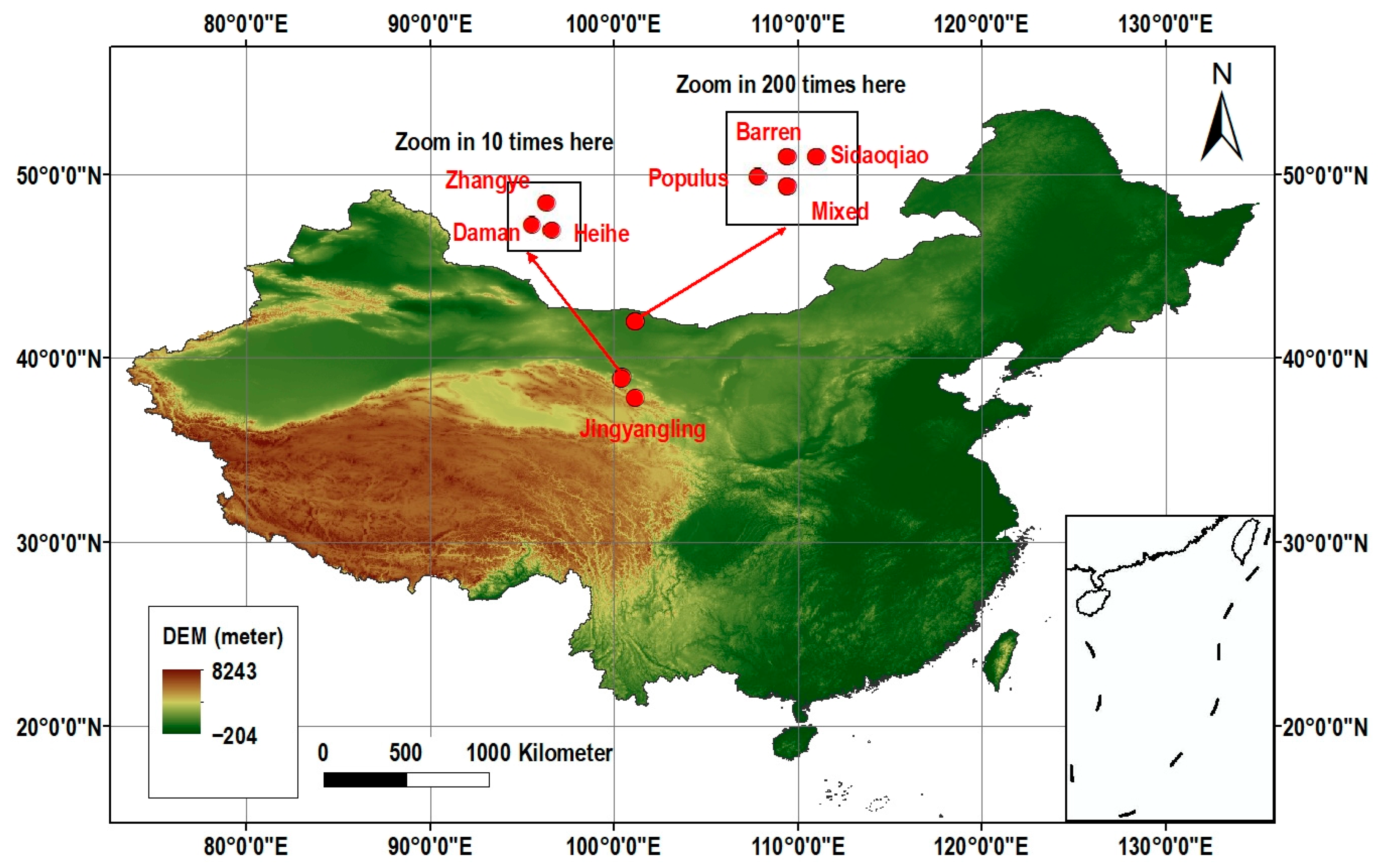
We selected the regions with ground validation stations as our study area, including the Heihe River Basin in China and the Mainland United States. The Heihe River Basin is located in Western China, approximately between 98° to 101°30′E longitude and 38° to 42°N latitude. It represents the largest inland river basin in the western part of Gansu and Inner Mongolia. It is characterized by arid conditions, scarce and concentrated precipitation, intense solar radiation, and significant diurnal temperature variations. The mainland of the United States is situated in North America, between approximately 24°N and 49°N latitude and between 67°W and 125°W longitude. The climate conditions vary across the country, ranging from arid and semi-arid in the Southwest to humid subtropical in the Southeast, with continental and maritime influences in different regions.

2.2. Obtaining and Preprocessing Data

The study employed satellite observations and station measurements. The following is a detailed introduction.

2.2.1. Satellite Data

In this study, we utilized the MODIS/Aqua daily level 3 LST dataset (MYD11A1, Collection 6). This particular dataset offers a spatial resolution of 1 km and is derived from MODIS bands 31 and 32, employing the split-window algorithm [3]. Our selection focused on MYD11A1, which captures daytime and nighttime observations at approximately local times of 13:30 and 1:30, respectively.
We also utilized passive microwave LST data from the Advanced Microwave Scanning Radiometer 2 (AMSR2), which is carried by the Aqua satellite manufactured by the National Aeronautics and Space Administration (NASA) of the United States. AMSR2 is a microwave radiometer with multiple frequencies that is designed to measure faint microwave emissions originating from the Earth’s surface and atmosphere. The AMSR2 level 3 high-resolution LST product was selected, which stores the daily LST derived from level 1B data at a spatial resolution of 10 km.
For obtaining normalized difference vegetation index (NDVI) data, we opted for the MODIS/Aqua 16-day vegetation index product (MYD13A2, Collection 6) with 1 km resolution. Within the MYD13A2 product, there are a total of 23 NDVI datasets available, covering the entire year of 2015. As the NDVI product is not available on a daily basis, this paper utilized the NDVI obtained on the day closest to the target day to represent the NDVI of the target date.
The Shuttle Radar Topography Mission (SRTM) Digital Elevation Data were employed for the digital elevation model (DEM). The SRTM dataset offers consistent elevation at a 90 m resolution. In order to achieve the desired resolution, we resized the DEM data from 90 m to 1 km by using nearest-neighbors interpolation.
The satellite data can be obtained from the websites provided in References [48,49,50]. We downloaded, projected, mosaicked, and cropped the MODIS LST, MODIS NDVI, and SRTM DEM datasets by using Google Earth Engine [51], and we processed the AMSR LST accordingly, using MATLAB 2021.

2.2.2. In Situ Data

Since the method in this paper is used to reconstruct real LST, it was necessary to use ground site measurements to verify the results. We used the Heihe sites in the Chinese mainland and the surface radiation budget network (SURFRAD) sites in the US as ground verification sites.
The Heihe River Basin, located in Western China, had diverse natural landscapes and was an ideal location for conducting research on land surface hydrological and ecological processes. The Heihe integrated observatory network was first established in 2007, during the Watershed Allied Telemetry Experimental Research (WATER) experiment, and was completed in 2013, during the Heihe Watershed Allied Telemetry Experimental Research (HiWATER) experiment. The Heihe stations monitored surface fluxes, soil moisture, wind speed, etc. The maximum collection rate of the measuring instrument can be once every 10 min. This study utilized measurements from eight Heihe River stations in 2015 (Appendix A Table A1 and Figure A1). These monitoring data were provided by the Heihe Plan Data Management Center of the National Natural Science Foundation of China [52,53].
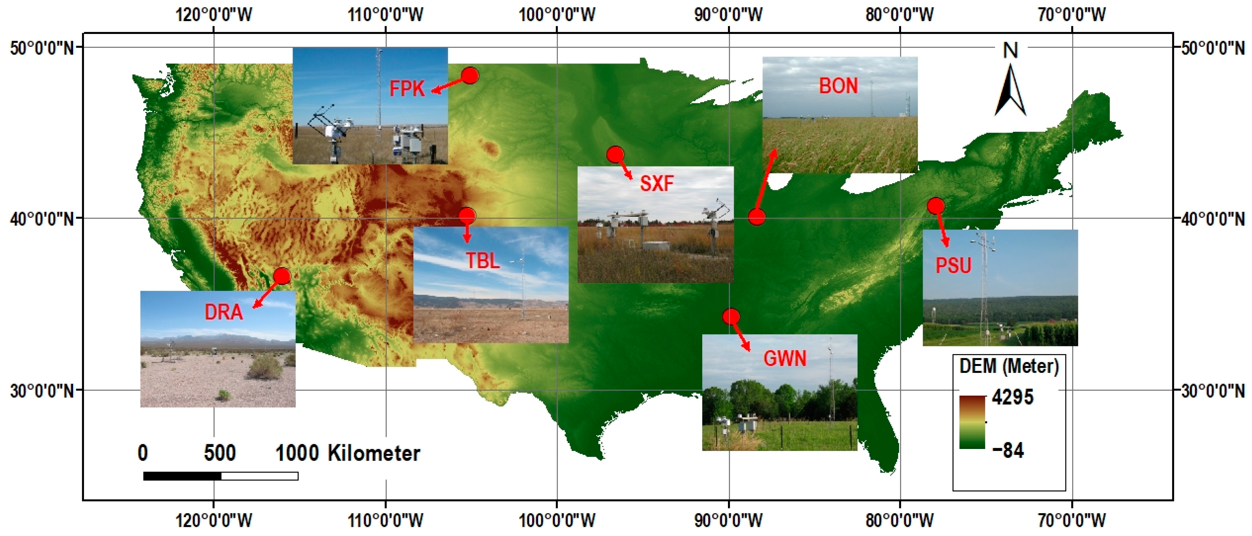
In addition to the Heihe sites, the SURFRAD sites were also used in the discussion section of this article. National Oceanic and Atmospheric Administration (NOAA) support enabled SURFRAD to be established. The SURFRAD sites give high-quality measurements that have been available every minute since 2009. A total of six SURFRAD sites were selected, and the corresponding information and photos can be found in Appendix A Table A2 and Figure A2.
It is necessary to convert all outgoing and incoming radiation from both Heihe and SURFRAD into LST before using them.
L S T = L o 1 ε b × L i ε b × σ 1 / 4
where L o denotes the observed longwave radiation from upwelling, L i denotes the observed longwave radiation from downwelling, and σ denotes the Stefan–Boltzmann constant ( 5.67 × 10 8   W m 2 K 4 ). Moreover, based on narrowband-to-broadband linear conversion, we can calculate surface broadband emissivity, ε b , using the following equation:
ε b = 0.2122 ε 29 + 0.3859 ε 31 + 0.4029 ε 32
where ε 29 , ε 31 , and ε 32 denote MODIS bands 29, 31, and 32 narrow-band emissivities, respectively. For the above two sets of site measurements, Heihe data were used in the accuracy assessment, and SURFRAD data were used in the discussion.

2.3. Method

In order to reconstruct the daily seamless real LST with 1 km spatial resolution in a large area, this study proposed a real LST reconstruction method combining Thermal Infrared and Microwave Remote Sensing Based on Temperature Conservation (TMTC).
The TMTC method combined microwave AMSR2 LST with thermal infrared MODIS LST and utilized the clear-sky LST obtained in previous studies to obtain the daily seamless real LST [25]. The method was divided into two steps: The first step involved filling in the orbital gaps and missing values in the microwave data AMSR2 LST. In the second step, the seamless 10 km AMSR2 LST obtained in the first step was downscaled to 1 km LST, while keeping the temperature unchanged at each AMSR2 pixel scale before and after reconstruction. The specific implementation of the two-step TMTC method is described below.

2.3.1. TMTC Step 1: AMSR2 LST Gap Filling

Microwave observation can penetrate the clouds to observe the real surface temperature. However, due to the influence of orbital gap, there are missing values. Therefore, the first step of the TMTC method was to fill in the gap with the microwave AMSR2 LST product with a spatial resolution of 10 km (Figure 1).
Taking a target pixel with no AMSR2 LST observation during the daytime as an example, if this pixel had AMSR2 LST observations on the previous and following day, Equation (3) was used to calculate its value.
L S T o b j e c t = m e a n ( L S T o b b ) m e a n ( L S T b e s ) × L S T b e f o r e + m e a n ( L S T o b a ) m e a n ( L S T a f s ) × L S T a f t e r / 2
L S T o b j e c t denotes the LST of the target pixel, L S T b e f o r e is the LST of the target pixel on the previous day, and L S T a f t e r is the LST of the target pixel on the following day. Moreover, m e a n ( L S T o b b ) denotes the mean LST on the target date of all pixels that have LST observations available for both the target date and the previous day’s images, and m e a n ( L S T b e s ) denotes the mean LST on the previous day of all pixels that have LST observations available for both the target date and the previous day’s images. Similarly, m e a n ( L S T o b a ) denotes the mean LST on the target date of all pixels that have LST observations available for both the target date and the following day’s images, and m e a n ( L S T a f s ) is the mean LST on the following day. If the target pixel has an AMSR2 LST observation available only on the previous day, it is calculated using Equation (4). If the observation is available only on the following day, it is calculated using Equation (5).
L S T o b j e c t = m e a n ( L S T o b b ) m e a n ( L S T b e s ) × L S T b e f o r e
L S T o b j e c t = m e a n ( L S T o b a ) m e a n ( L S T a f s ) × L S T a f t e r
The variables in Equations (4) and (5) have the same meanings as those in Equation (3). Finally, if the target pixel has no observation available on either the previous or the following day, the AMSR2 monthly average LST product is used for gap-filling, according to Equation (6).
L S T o b j e c t = m e a n ( L S T o b m ) m e a n ( L S T m o s ) × L S T m o n t h
Similar to the three formulas above, L S T m o n t h represents the value of the target pixel of the AMSR2 monthly average LST product, m e a n ( L S T m o s ) represents the average LST of all intersecting pixels between the target date LST and the monthly average LST on the monthly average LST image, and m e a n ( L S T o b m ) represents the average LST of these intersecting pixels on the target date LST image. By using the AMSR2 LST data of adjacent dates and the same month for all target pixels (the calculation method for nighttime LST was the same as for daytime), the missing LST values for all pixels can be calculated, and all the orbital gaps can be filled to obtain a seamless and complete 10 km resolution daily real LST.

2.3.2. TMTC Step 2: AMSR2 LST Downscaling

The first step of the TMTC method provided seamless daily 10 km LSTs. The second step involved the use of MODIS LST and the 1 km seamless clear-sky LST to downscale the LST from a 10 km to 1 km resolution. Figure 2 illustrates the specific process.
Taking an example of an AMSR2 LST pixel on the target date, if all 100 MODIS LST pixels covered by this pixel were known, that is, all the 100 pixels had MODIS LST observations, their MODIS LSTs would be directly taken as the final result. If all 100 MODIS LST pixels within the AMSR2 pixel were unknown, that is, all were cloudy-sky pixels without MODIS LST observations, then each cloudy-sky pixel, i, was calculated using Equation (7).
L S T r e a l 1 ( i ) = 100 × L S T B M E ( i ) i = 1 100 L S T B M E ( i ) × L S T r e a l 10
L S T r e a l 1 ( i ) represents the 1 km resolution real LST of the i-th cloudy-sky pixel to be solved; and L S T r e a l 10 represents the 10 km real LST, which is calculated in the first step. L S T B M E ( i ) represents the clear-sky LST of the i-th pixel obtained from the Bayesian maximum entropy (BME) method [25], and i = 1 100 L S T B M E ( i ) represents the sum of clear-sky LST values of the 100 cloudy-sky pixels. In fact, L S T r e a l 10 can be understood as the average LST of the 100 cloudy-sky pixels, and 100 × L S T B M E ( i ) i = 1 100 L S T B M E ( i ) can be understood as the weight of the i-th pixel.
The above two scenarios described the cases where all MODIS pixels within an AMSR2 pixel are either known clear-sky pixels or unknown cloudy-sky pixels. The last scenario is when some MODIS pixels within an AMSR2 pixel were clear-sky and others were cloudy-sky. Assuming there are m clear-sky pixels with MODIS LST observations, there are 100-m unknown cloudy-sky pixels. The equation for calculating the LST of the i-th cloudy-sky pixel is given as follows.
L S T r e a l 1 ( i ) = ( 100 m ) × L S T B M E ( i ) i = 1 100 m L S T B M E ( i ) × L S T r e a l 10 × 100 j = 1 m L S T M O D ( j ) 100 m
Similarly, L S T r e a l 1 ( i ) denotes the 1 km real LST of the i-th cloudy-sky pixel to be solved; L S T r e a l 10 is the LST value of the AMSR pixel; L S T M O D ( j ) is the MODIS LST value of the j-th clear-sky pixel; j = 1 m L S T M O D ( j ) is the sum of MODIS LST values of m clear pixels; i = 1 100 m L S T B M E ( i ) is the sum of clear-sky LST values of 100-m cloudy-sky pixels; and L S T r e a l 10 × 100 j = 1 m L S T M O D ( j ) 100 m , to the right of the multiplication sign, denotes the mean LST of the 100-m cloudy-sky pixels. Moreover, ( 100 m ) × L S T B M E ( i ) i = 1 100 m L S T B M E ( i ) , to the left of the multiplication sign, denotes the LST weight of the i-th cloudy-sky pixel.
Here is a brief introduction to the BME method mentioned above. The BME clear-sky LST reconstruction method involved inputting hard data, soft data with uncertainty, and a covariance model into the BME algorithm. For the hard data input, we utilized the difference between the MODIS observed LST and the mean LST of a 15-day period. The soft data input consisted of a Gaussian distribution of LSTs calculated using auxiliary information such as NDVI and DEM. Subsequently, the daily spatial covariance coefficients were calculated. Finally, these three types of data were fed into the BME method to obtain the reconstructed BME clear-sky LST. The calculation process closely followed Zhang’s work [25].
In summary, the downscaling method in the second step of TMTC first judged each AMSR LST pixel. When all 100 MODIS LST pixels within the AMSR pixel were clear-sky pixels, the MODIS LSTs were directly used as the resulting LSTs. When all 100 MODIS LST pixels were cloudy-sky pixels, Equation (7) was used to calculate the reconstructed LST. When some of the 100 MODIS LST pixels were clear-sky and some were cloudy-sky pixels, Equation (8) was used to calculate the reconstructed LST. It can be seen that when all or part of the 100 MODIS pixels within an AMSR pixel were cloudy-sky pixels, the reconstructed mean LST of these 100 pixels was equal to the LST of the AMSR pixel. The steps for daytime and nighttime were the same, and 1 km seamless daily real LSTs for both daytime and nighttime were obtained using the TMTC method.
The TMTC method combined microwave LST and thermal infrared LST data. Under clear-sky conditions, the MODIS LST with higher accuracy was directly used, while under cloudy-sky conditions, the TMTC method used the magnitude of the clear-sky LST values to distribute the high and low fluctuations of the resulting LSTs, while maintaining the average LST temperature of each AMSR2 pixel unchanged. The assumptions of the TMTC method included the following: (1) the assumption of precise synchronization of observation times between AMSR2 LST and MODIS LST (MYD11A1) twice a day; and (2) the assumption of acceptable accuracy for the 10 km AMSR2 LST product and the 1 km MODIS LST product.

3. Results

3.1. Spatial Display of Results LSTs

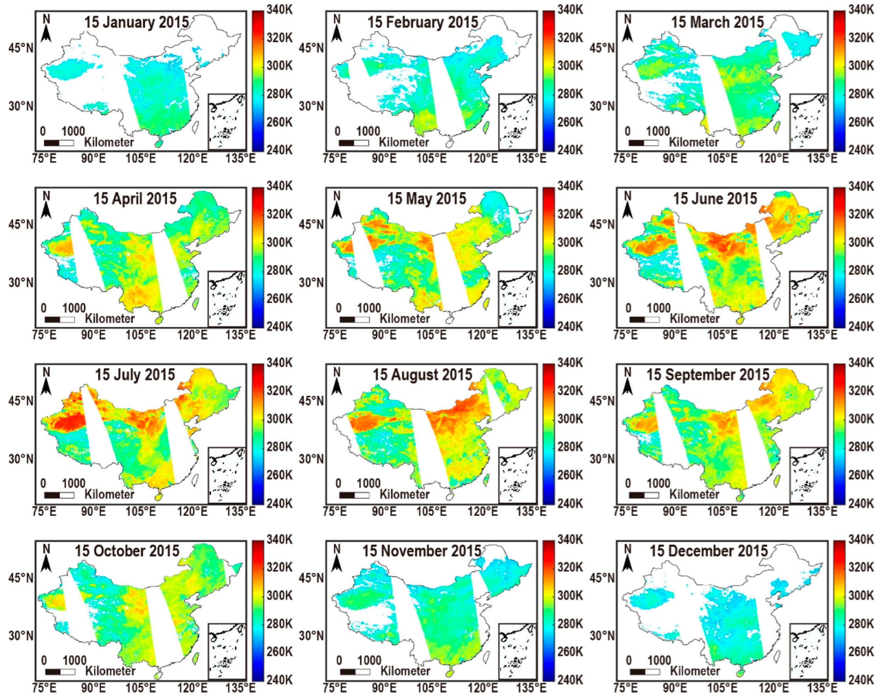
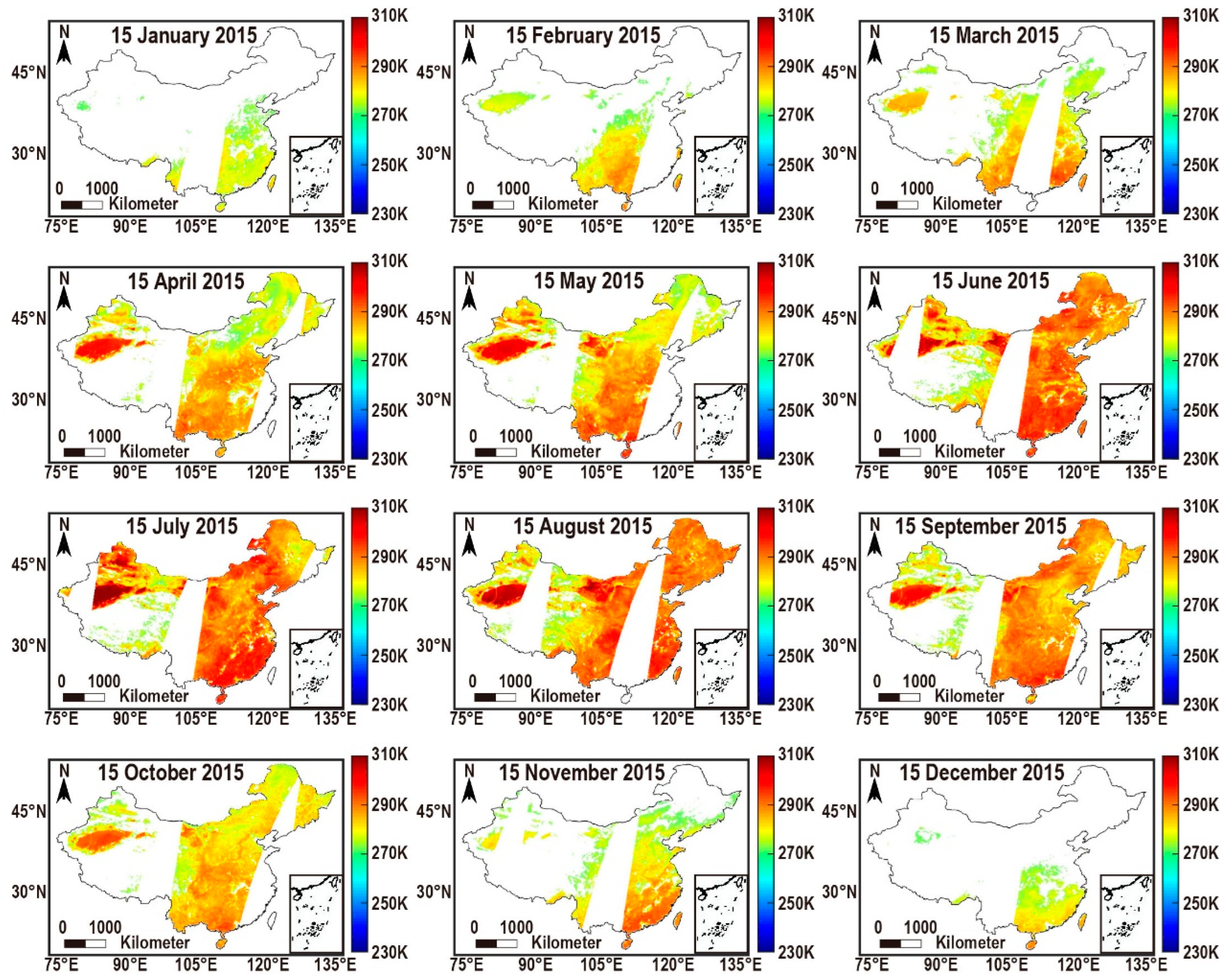
The AMSR2 orbital gaps were evenly spaced but appeared at different locations on different dates (Figure 3 and Figure 4). In fact, due to the orbital path of GCOM-W1/AMSR2, the observation data were segmented into “granules”, which were defined as half orbits between the North Pole and the South Pole. The ascending granule scene was scanned from the southernmost to the northernmost half-orbit, corresponding to daytime observations (Figure 3), while the descending granule scene was scanned from the northernmost to the southernmost half-orbit, corresponding to nighttime observations (Figure 4). One ascending granule and one descending granule combined to form an orbital path. AMSR2 had 233 different orbital paths that seamlessly covered the globe, with nearly 15 paths with gaps covering the globe each day. The satellite had a revisiting cycle of 16 days, meaning that the interval time to revisit the same location was 16 days. That is to say, the positions of orbital gaps on adjacent two days were different. Therefore, the TMTC method proposed in this study first used the observations on adjacent two days before and after to fill the gaps. Then, if there was still a small mumber of gaps, the average monthly data were used to fill in the gaps.
In the Chinese mainland, the missing rate of observations due to AMSR2 orbital gap accounted for about 25% to 50%, which was lower than the missing rate caused by cloud coverage in MODIS observations, and the missing distribution of the former was uniform, while that of the latter was not. In other words, the missing quantities and distributions of the microwave LST and thermal infrared LST are different, and there is a complementary relationship between them. Therefore, it is feasible to combine these two types of LST to reconstruct a seamless real LST.
Figure 5 and Figure 6 show the daytime and nighttime LST distribution of 2015 for the 15th day of every month, as reconstructed by TMTC, corresponding to Figure 3 and Figure 4, respectively. As can be seen from the completeness, the TMTC method can fill in the missing pixels 100%, realizing the seamless spatial reconstruction of real LST. The reconstructed LST showed no obvious seam marks at the gaps, indicating a natural transition effect of TMTC method. In addition, the TMTC method had a good ability to describe spatial heterogeneity, and the spatial distribution of the reconstructed LST corresponded to the annual variation of LST in the Chinese mainland.

3.2. Accuracy Assessment

In this study, we employed several evaluation metrics to assess the performance of the TMTC method. These metrics included the Mean Absolute Error (MAE), which measures the average absolute difference between the predicted and actual LSTs; Root Mean Square Error (RMSE), which calculates the square root of the average of the squared differences between the predicted and actual LSTs; and Coefficient of Determination (R2), which represents the proportion of the variance in the actual LSTs that can be explained by the predicted LSTs. The term “predicted LSTs” mentioned in the aforementioned accuracy assessment refers to the reconstructed real LSTs obtained through the TMTC method. Conversely, the term “actual LSTs” refers to the ground-truth LSTs collected on-site for validation purposes.
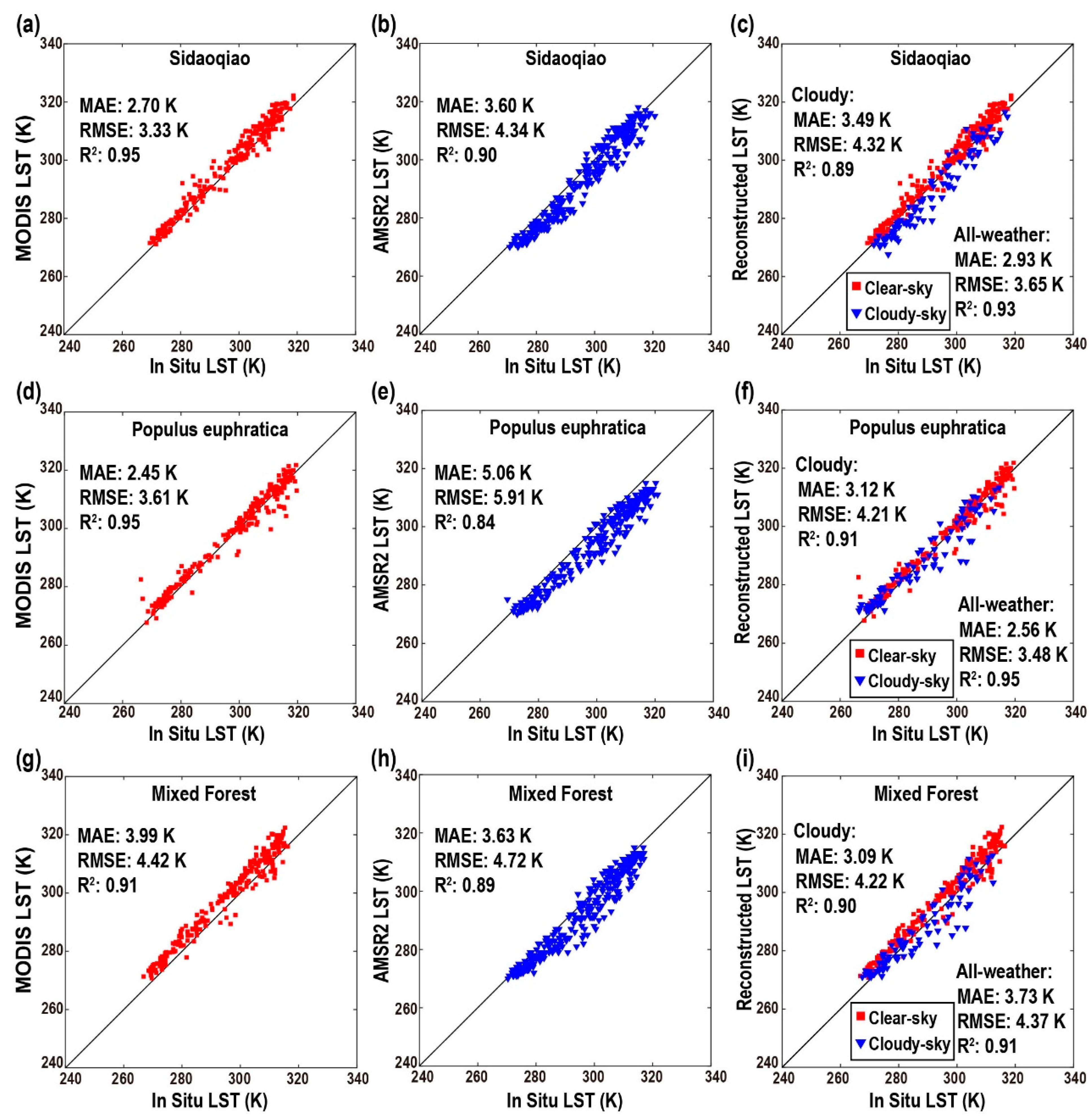
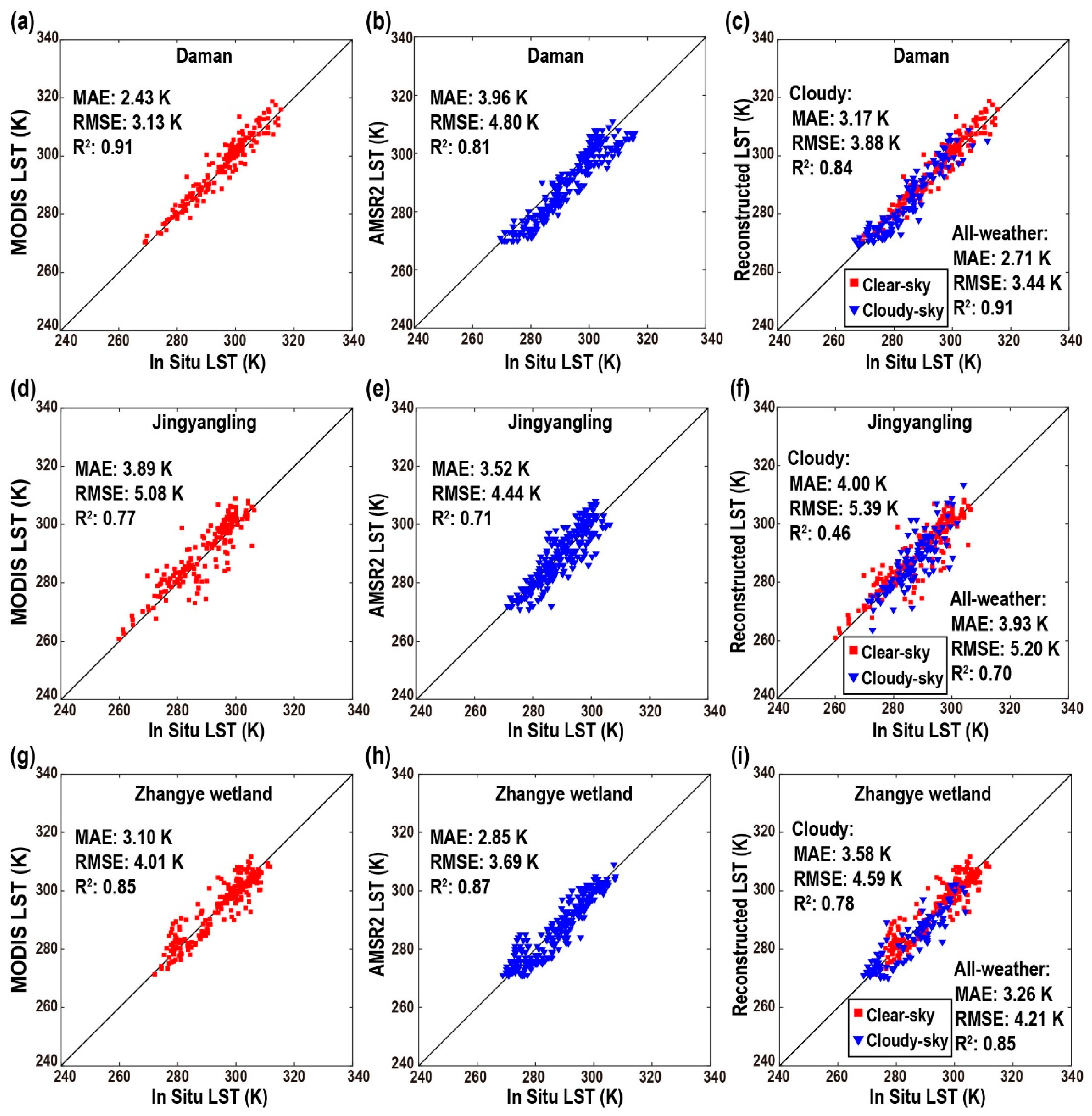
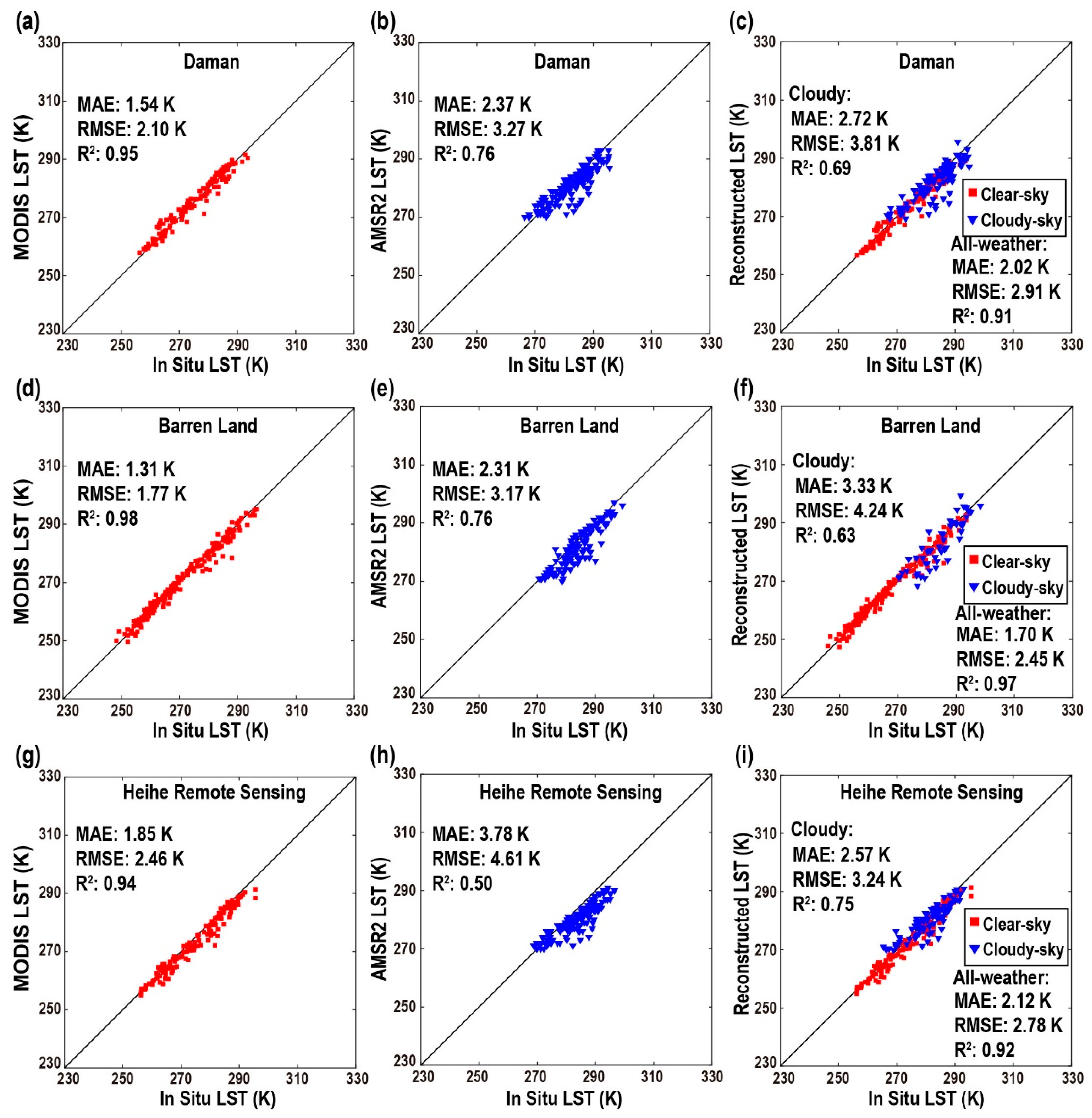
Since the TMTC method reconstructed the real LST, it was necessary to verify the results by using actual measurements from ground stations. In this section, we selected measurements from the Heihe stations in the Chinese mainland for validation, and their detailed introduction and processing method can be found in Section 2.2.2. Due to data quality issues, six stations were selected for validation during the daytime and nighttime each. The daytime stations were Sidaqiao, Populus euphratica, Mixed Forest, Daman, Jingyangling, and Zhangye wetland (Figure 7 and Figure 8), while the nighttime stations were Sidaqiao, Populus euphratica, Mixed Forest, Daman, Barren Land, and Heihe Remote Sensing (Figure 9 and Figure 10). The first four stations were the same for both daytime and nighttime, while the last two stations were different.
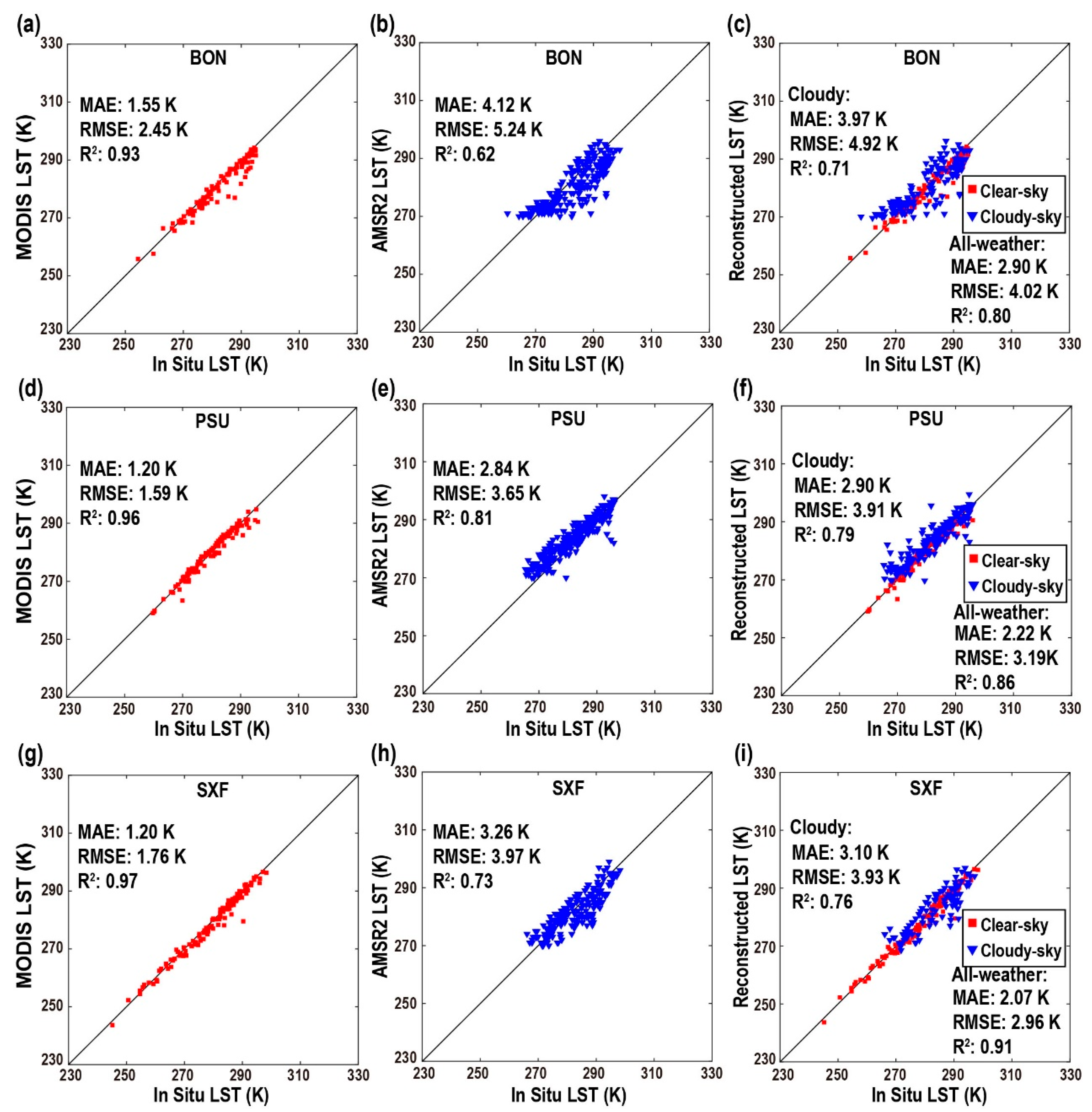
The accuracy of all scatter plots was calculated using the in situ LST value as the reference value. Each row in the plots represented a single station, and one dot represented the the daytime in 2015. Taking Sidaoqiao Station as an example, Figure 7a shows the scatter plot of MODIS LST versus in situ LST during the clear-sky dates in 2015, with the corresponding MAE, RMSE, and R2. Figure 7b shows the scatter plot of AMSR2 LST versus in situ LST during the daytime when microwave observations are available at the site, and the corresponding MAE, RMSE, and R2 are given. Figure 7c displays the scatter plot of all reconstructed real LST and in situ LST after using the TMTC method. Among them, the red square points represented clear-sky points, which were directly equal to the MODIS LST values in the TMTC method. The blue triangle points represented cloudy-sky points, which were equal to the reconstructed real LST values in the TMTC method. The MAE, RMSE, and R2 in the upper left corner of the figure were the accuracy of these blue triangle points, that is, the accuracy of all non-clear-sky pixels. The MAE, RMSE, and R2 located in the lower right corner in the figure showed the accuracy of the combined blue and red points, that is, the overall accuracy of all clear-sky and non-clear-sky pixels, representing the overall accuracy of the TMTC method at this station throughout the year.
Therefore, the first column of Figure 7 and Figure 8 represented the accuracy of MODIS LST product, the second column represented the accuracy of AMSR LST product, and the third column represented the accuracy of reconstructed real LST using the TMTC method. The average MAE, RMSE, and R2 of MODIS LST for the six selected stations were 3.09 K, 3.93 K, and 0.89, respectively. The corresponding accuracy of AMSR2 LST was 3.77 K, 4.65 K, and 0.84, indicating that the error of AMSR2 LST was larger than that of MODIS LST. The cloudy-sky mean MAE, RMSE, and R2 of the six sites were 3.41 K, 4.44 K, and 0.80, respectively, and the all-weather mean MAE, RMSE, and R2 were 3.19 K, 4.06 K, and 0.88, respectively. The accuracy of cloud was closer to that of AMSR2 LST, while the all-weather accuracy was affected by both MODIS and AMSR2. For Jingyangling Station (Figure 8d–f), the errors between MODIS versus the in situ value and AMSR2 versus the in situ value were both large, and the accuracy of cloud-sky and all-weather was the lowest, which was caused by the special situation of abnormal values in the site measurements. During the daytime, the ranking of all-weather accuracy for various land-cover types from high to low was Populus euphratica, tamarix, maize, mixed forest, reed, and alpine meadow.
The meaning of the nighttime scatter plots was the same as that of the daytime scatter plots (Figure 9 and Figure 10). The average MAE, RMSE, and R2 of the MODIS LST were 1.98 K, 2.48 K, and 0.95, respectively, while the corresponding accuracies of AMSR2 LST were 2.58 K, 3.37 K, and 0.73, respectively. The MODIS accuracy was higher for the nighttime than the daytime, while the AMSR2’s MAE and RMSE accuracies were also higher for the nighttime than the daytime, but its R2 was lower for the nighttime than the daytime. Both daytime and nighttime MODIS LST accuracies were significantly higher than those of AMSR2 LST. The nighttime average MAE, RMSE, and R2 of the six stations were 2.89 K, 3.74 K, and 0.71 for cloudy conditions and 2.24 K, 2.92 K, and 0.94 for all-weather conditions. The lower accuracy of AMSR2 LST for the nighttime resulted in the lower accuracy of the cloudy-sky LST calculated using the TMTC. However, the all-weather accuracy for the nighttime was high due to the high MODIS LST accuracy and the large number of clear-sky days at these sites for the nighttime.
During the nighttime, the ranking of the all-weather LST accuracy of various land-cover categories from high to low was barren land, mixed forest, tamarix, grassland, Populus euphratica, and maize. It can be seen that mixed forest and tamarix had high accuracy both for the daytime and nighttime. In addition, the daytime relative accuracies of maize and Populus euphratica were higher than those for the nighttime.

4. Discussion

4.1. Accuracy in Other Regions

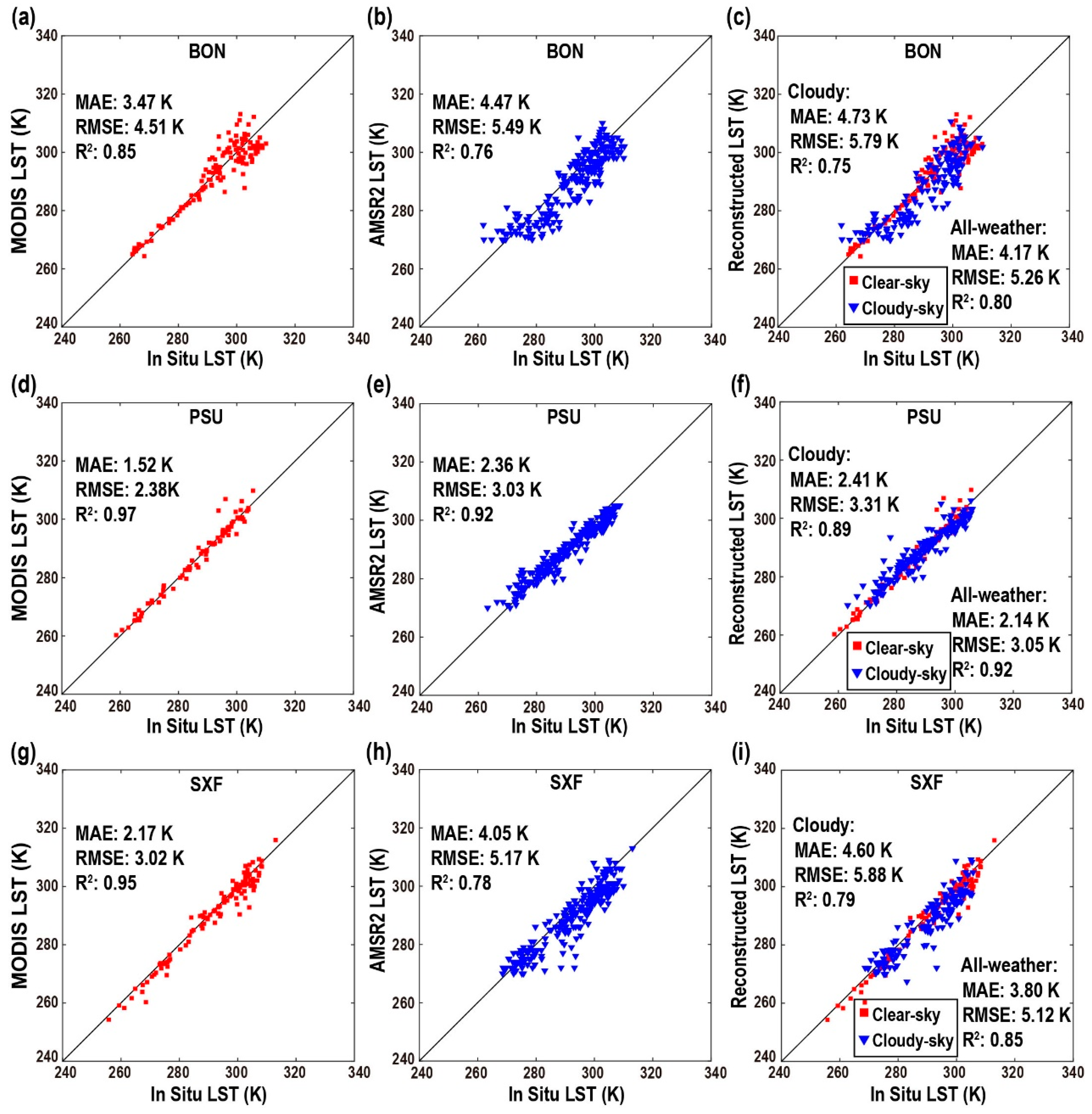
In the Section 3, the model was already validated in the Chinese mainland region. This section aimed to verify the spatial generality and practicability of the TMTC method by conducting accuracy validation in the United States. Six SURFRAD sites were selected for this purpose: GWN, TBL, FPK, BON, PSU, and SXF. The land-cover types for GWN, TBL, and FPK were grasslands, while those for BON, PSU, and SXF were croplands.
The scatter plots for daytime (Figure 11 and Figure 12) and nighttime (Figure 13 and Figure 14) had the same meaning as Figure 7, Figure 8, Figure 9 and Figure 10. During the daytime, the average MAE, RMSE, and R2 for the MODIS LST at the six sites were 2.37 K, 3.21 K, and 0.92, respectively, while the corresponding values for the AMSR2 LST were 3.36 K, 4.24 K, and 0.85. The accuracy of MODIS LST was higher than that of AMSR2 LST. The average MAE, RMSE, and R2 for cloudy conditions were 3.63 K, 4.70 K, and 0.83, respectively, while the corresponding values for all-weather conditions were 3.09 K, 4.13 K, and 0.88, respectively. At the BON site in Figure 12, both the MODIS LST and the AMSR2 LST had relatively large errors, resulting in the lowest accuracy for both cloudy-sky and all-weather LST reconstructed by TMTC among the six sites. Regarding types of land cover, the accuracy of grasslands was higher than that of croplands. Moreover, the accuracies of the MODIS, the AMSR2 and the reconstructed LSTs showed no outliers at all sites, indicating that the SURFRAD measurements had smaller and more stable errors than the Heihe measurements.
During the nighttime, the average MAE, RMSE, and R2 of the MODIS LST at the six sites (Figure 13 and Figure 14) were 1.56 K, 2.25 K, and 0.94, respectively, while the corresponding accuracy values for AMSR2 LST were 3.75 K, 4.47 K, and 0.66. The MODIS accuracy was higher for the nighttime than for the daytime, while the AMSR2 accuracy was lower at night than during the day. However, the accuracy of both MODIS LSTs during the daytime and nighttime was significantly higher than that of AMSR2 LST, as is consistent with the results for the Chinese mainland. The average MAE, RMSE, and R2 for cloudy conditions were 3.27 K, 4.33 K, and 0.70, respectively, while the corresponding values for all-weather conditions were 2.43 K, 3.47 K, and 0.86, respectively. The accuracy of the cloudy-sky LST for the nighttime was low, and the R2 of the all-weather LST was also slightly lower than that of the daytime, and this was caused by the lower AMSR2 LST accuracy for the nighttime. During the nighttime, the accuracy of cropland classification exhibited a generally higher level compared to that of grassland, which was different from daytime. This was because the reconstructed cloudy and all-weather accuracy were jointly affected by the accuracy of MODIS and AMSR2. For the daytime, the accuracy of grassland was slightly higher, while for the nighttime, the accuracy of cropland was slightly higher.
Overall, based on the ground-station validation accuracy, during the daytime, the MODIS LST validation accuracy in the US was higher than in the Chinese mainland, while the AMSR2 LST validation accuracy was similar in both regions, and the reconstructed cloudy and all-weather LST accuracies were also similar between the two regions. There were no anomalous values observed in the US station measurements. During the nighttime, the MODIS LST validation accuracy was similar between the two regions, while the AMSR2 LST validation accuracy was lower in the US than in the Chinese mainland, resulting in lower reconstructed cloudy and all-weather LST accuracy in the US than in the Chinese mainland. In general, in both regions, the MODIS validation accuracy was higher than that of the AMSR2, the MODIS validation accuracy was higher during the nighttime than during the daytime, and the AMSR2 validation accuracy was lower during the nighttime than during the daytime. The accuracy of the TMTC method in reconstructing cloudy LST was mainly affected by the accuracy of AMSR2, while the all-weather LST accuracy was simultaneously affected by the accuracy of both MODIS and AMSR2. It can be seen from the verification results that the TMTC method has spatial generality and practicability.

4.2. Simplified TMTC

The TMTC method proposed in this study required the use of the clear-sky LST reconstructed using the BME method. Since all methods for reconstructing the clear-sky LST are complex, this section proposes a real LST reconstruction method that does not rely on clear-sky LST data, called the Simplified TMTC method, and compares its accuracy with that of the TMTC method.
The Simplified TMTC method was similar to the TMTC method. In the first step, the gap-filling of microwave LST remained unchanged. In the second step, the regression LST was used instead of the clear-sky LST; that is, TMTC used the clear-sky LST to downscale microwave LST, while the Simplified TMTC used the regression LST to downscale microwave LST. The regression-based LST was obtained by performing a multiple linear regression between MODIS LST and four independent variables, namely NDVI, DME, longitude, and latitude, and all were processed to 1 km resolution. As these four independent variables had complete spatial coverage, the resulting regression LST was also spatially complete and could be used to replace clear-sky LST.
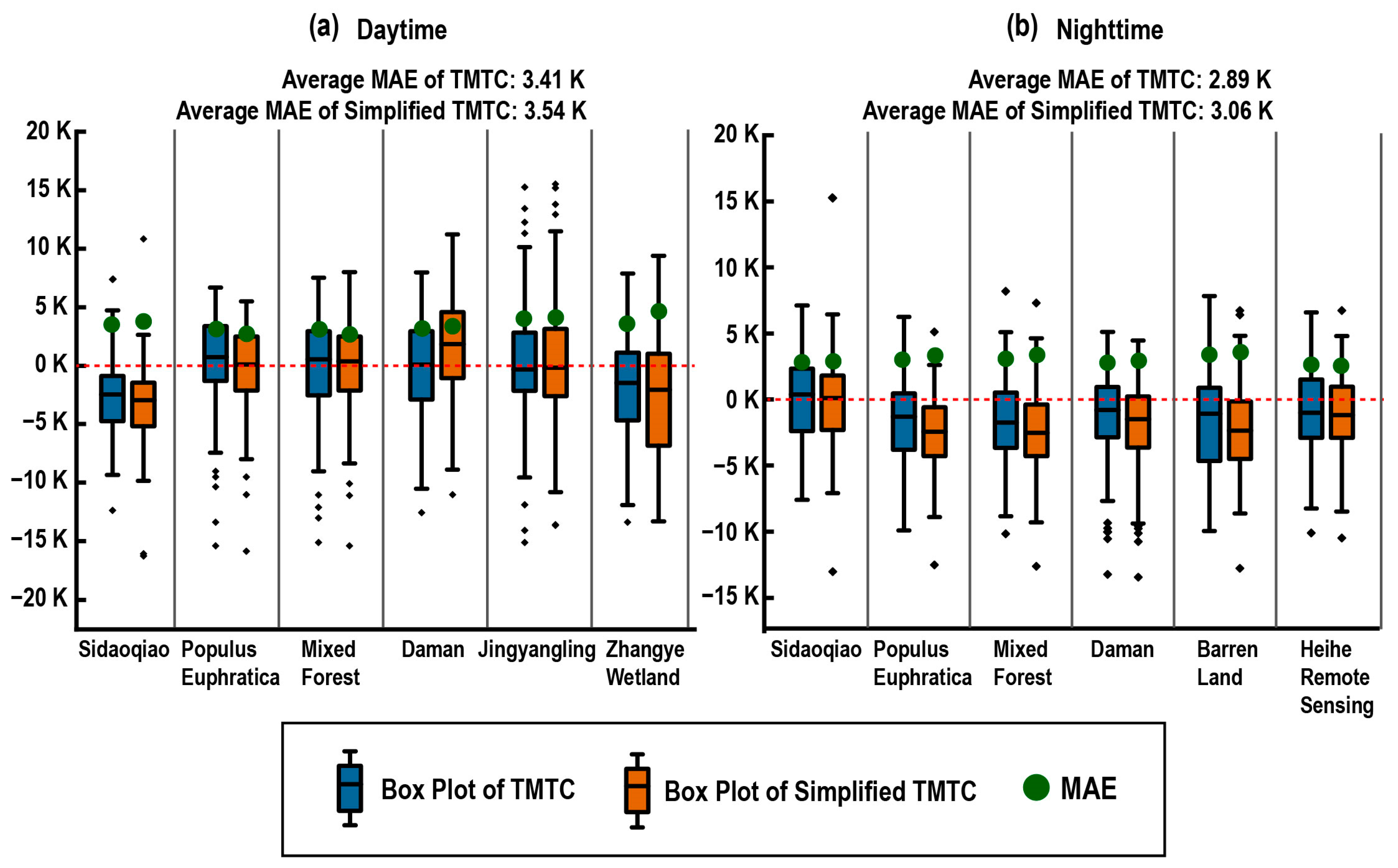
We compared the accuracy of the Simplified TMTC and the TMTC by using the measurements at six sites for both daytime and nighttime in Heihe in 2015 (Figure 15). Overall, the Simplified TMTC method was slightly less accurate than the TMTC method, with a difference of 0.13 K in MAE during the daytime and 0.17 K in MAE during the nighttime. The Simplified TMTC method had higher accuracy at the Populus euphratica and mixed forest stations for the daytime, while the TMTC method had higher accuracy at the other stations, with box plots distributed closer to 0 K. In addition, the average MAE of both methods was over 3 K for the daytime, while TMTC’s MAE was less than 3 K for the nighttime, and Simplified TMTC’s MAE was over 3 K. Therefore, the Simplified TMTC method that does not rely on clear-sky LST data was simpler in regard to its steps but slightly less accurate than the TMTC method.

4.3. Exploration of the Accuracy Improvement (Ideal Accuracy of TMTC)

The real LST reconstructed by the TMTC method was validated using measurements from actual monitoring stations. The average MAE and RMSE for a total of 12 stations, including the six Heihe stations in China and six SURFRAD stations in the US, during the daytime were 3.14 K and 4.10 K, respectively, with corresponding ranges of 2.14 K to 4.17 K and 3.05 K to 5.26 K. During the nighttime, the average MAE and RMSE for the 12 stations were 2.34 K and 3.20 K, respectively, with corresponding ranges of 1.70 K to 3.41 K and 2.45 K to 4.02 K. In previous studies on reconstructing real LST, Duan achieved an RMSE of 3.46 K to 4.36 K, using data from four stations in the Heihe region, while Zeng obtained an MAE of 3 K to 6 K, using data from six SURFRAD stations in the United States. Therefore, the TMTC method demonstrates comparable or slightly higher accuracy than that of previous research [35,44].
Most of the errors in the TMTC method were caused by the temporal coincidence of MODIS and AMSR2 LST observations. The error test in Section 3.2 and Section 4.1 included errors due to time inconsistency, while this section aimed to calculate the ideal accuracy that could be achieved by the TMTC method under the condition that MODIS and AMSR2 have completely consistent observation times. Since the temporal normalization process was complex, this section used the aggregated MODIS LST to simulate the AMSR2 LST for accuracy validation, which can be regarded as the ideal situation, wherein the observation time of MODIS and AMSR2 was completely consistent. Since the Simplified TMTC method had a simpler calculation process and a similar accuracy to the TMTC method, it was used instead of the TMTC method in this section.
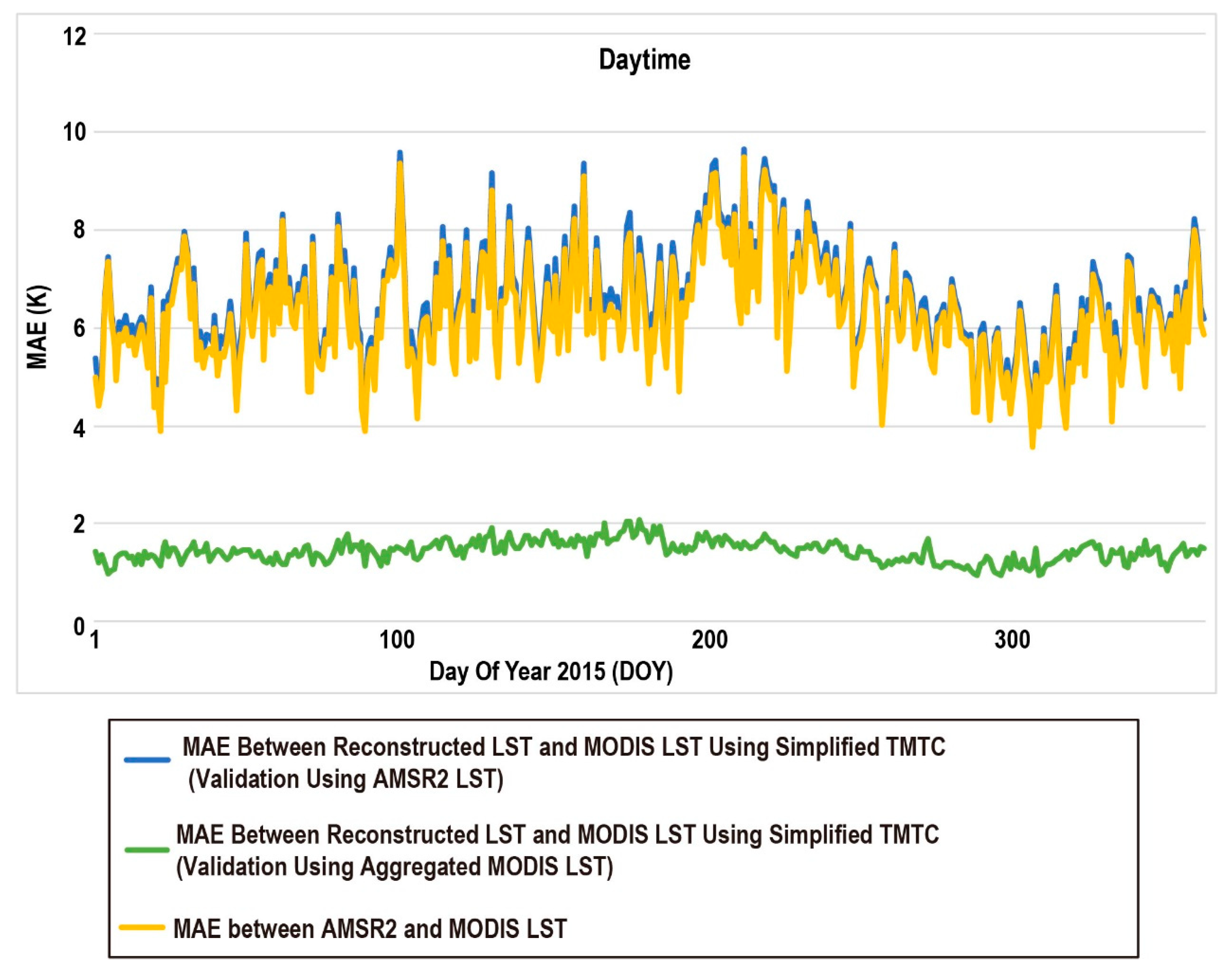
The specific steps of the validation were as follows: (1) Taking the daytime of a certain day in 2015 as an example, the 1 km resolution MODIS LST was aggregated into 10 km resolution LST, using the mean aggregation method. The aggregated MODIS LST was obtained by taking the average LST value of each 10 × 10 pixel window as the LST value of each pixel after aggregation. The positions of all 10 × 10 windows in the MODIS image corresponded to the positions of AMSR2 pixels. (2) The pixels that had values in both the AMSR2 image and the aggregated MODIS image were selected as the experimental pixels. (3) The three types of MAE were calculated for each experimental pixel. The first type of MAE represented the difference between the AMSR2 LST and the aggregated MODIS LST, which represented the error between the two datasets. The second type of MAE was calculated by using the Simplified TMTC method to downscale the aggregated MODIS LST to 1 km LST and calculating the MAE between the downscaled LST and the original MODIS LST. The third type of MAE was calculated by using the Simplified TMTC method to downscale the 10 km AMSR2 LST to 1 km LST and calculating the MAE between the downscaled LST and the original MODIS LST.
Figure 16 presented the time series of the three types of MAEs during daytime for all 365 days in 2015. All three MAEs were evaluated using the MODIS LST as the reference. The first MAE (yellow line) reflected the degree of proximity between the AMSR2 LST and MODIS LST. The second MAE (green line) reflected the ideal accuracy of the Simplified TMTC method, which can be considered as the accuracy when the observation times of AMSR2 and MODIS are completely synchronized. The third MAE (blue line in Figure 16) reflected the degree of proximity between the reconstructed 1 km real LST, using the Simplified TMTC method, and the MODIS LST under actual conditions.
The average MAE of the yellow line over 365 days was 6.25 K, indicating a large difference between daytime AMSR2 LST and MODIS LST values. This was mainly caused by the inconsistency in observation time and differences in the inversion accuracy of the two LST products. The blue line had an average MAE of 6.49 K, which was similar to the precision of the yellow line, indicating that, in practical applications, the accuracy of the downscaled AMSR2 LST is related to its proximity to the MODIS LST. That is, the closer the AMSR2 LST and MODIS LST observations are, the closer the reconstructed LST using the Simplified TMTC method will be to the MODIS LST. The green line had an average MAE of 1.43 K, representing the ideal accuracy achievable by the Simplified TMTC method. The aggregated MODIS LST can be regarded as a simulated AMSR2 LST, which has a consistent observation time with MODIS LST, and its inversion accuracy is greater than that of the real AMSR2 LST. The overall high accuracy of the green line suggests that the method of using auxiliary information (such as seamless clear-sky LST in TMTC and seamless regression LST in Simplified TMTC) to weight the AMSR2 LST for reconstruction of the real LST is reasonable.
In the nighttime, the same validation was performed (Figure 17). The yellow line showed the MAE between the original AMSR2 LST and MODIS LST, with a mean value of 4.66 K over 365 days. The blue line reflected the MAE between the reconstructed LST using the Simplified TMTC method and the MODIS LST, with a mean value of 4.74 K over 365 days, which is also very close to the yellow-line accuracy. The green line represented the MAE between the MODIS LST and the reconstructed LST, using the Simplified TMTC method, by downscaling the simulated LST, with a mean value of 0.79 K over 365 days, indicating that the ideal accuracy for the nighttime can be within 1 K. As the average LST during the nighttime is lower than that during the daytime, the three MAE values for the nighttime were correspondingly lower than those for the daytime.
In summary, it can be seen that the inversion accuracy of the AMSR2 LST product, the inversion accuracy of the MODIS LST product, and especially the closeness of the observation time between AMSR2 LST and MODIS LST largely affected the accuracy of the TMTC method. In future studies, we recommend improving the accuracy of MODIS LST and AMSR2 LST, especially by implementing prior time normalization for both LST products. This approach will greatly enhance the accuracy of the TMTC method. The ideal accuracy of the TMTC method reaches less than 1.5 K during the day and less than 1 K at night.

5. Conclusions

In this study, we proposed a real LST reconstruction method combining Thermal Infrared and Microwave Remote Sensing Based on Temperature Conservation (TMTC). This method combined microwave AMSR2 LST and thermal infrared MODIS LST and kept the temperature of the resulting LST and microwave LST unchanged on the microwave pixel scale. By using this method, the seamless daily real LST with a spatial resolution of 1 km in the Chinese mainland in 2015 was reconstructed. During the validation stage, the accuracy of the TMTC method was evaluated using the in situ measurements. The average MAE, RMSE, and R2 were 3.14 K, 4.10 K, and 0.88 for the daytime and 2.34 K, 3.20 K, and 0.90 for the nighttime, respectively. Then, we proposed a Simplified TMTC method which does not rely on the reconstructed clear-sky LST values, and its MAE for the daytime and nighttime were 0.13 K and 0.17 K higher than that of the TMTC method, respectively. The differences of product accuracy and observation time between AMSR2 and MODIS LST were the main factors affecting the accuracy of TMTC method.
The TMTC has the following advantages: (1) It can combine microwave data and thermal infrared data, while keeping the result LST and microwave LST consistent in pixel scale. (2) Compared with the commonly used real LST reconstruction methods based on surface energy conservation, the calculation process of this method is simple, and it can quickly reconstruct a complete real LST in a large area with acceptable accuracy.
There are also some limitations to this method: (1) The reconstructed LST by using the TMTC method may have small spatial noise due to the lack of temporal normalization between AMSR2 LST and MODIS LST, resulting in large differences between the MODIS clear-sky LST and the reconstructed cloudy-sky LST within certain AMSR2 pixels. (2) The accuracy of the method is influenced by the accuracy of the microwave AMSR2 LST product, which has a relatively low accuracy, with an RMSE of 3–6 K, thus limiting the improvement of the method’s accuracy.
The TMTC method can be used to reconstruct 1 km spatial resolution real LST over large areas, providing a basis for the spatiotemporal analysis of LST and its related applications. In addition, exploring the time normalization of AMSR2 LST and MODIS LST products can improve the accuracy of the method and make the fusion of microwave and thermal infrared remote sensing more reliable, which is a direction for future research.

Author Contributions

Conceptualization, Y.Z. and X.L.; data curation, Y.Z.; formal analysis, Y.Z.; funding acquisition, X.L.; investigation, Y.Z.; methodology, Y.Z. and X.L.; project administration, X.L.; resources, Y.Z.; software, Y.Z.; supervision, X.L.; validation, Y.Z.; visualization, Y.Z.; writing—original draft, Y.Z.; writing—review and editing, Y.Z., X.L., K.Z., L.W., S.C. and P.S. All authors have read and agreed to the published version of the manuscript.

Funding

This research was funded by the Natural Science Foundation of China, grant number 42271487 and grant number 41930109; and Beijing Outstanding Young Scientist Program, grant number BJJWZYJH01201910028032.

Data Availability Statement

All the satellite data utilized in this study are publicly available in public repositories.

Conflicts of Interest

The authors declare no conflict of interest.

Appendix A

Table A1. Eight land surface temperature (LST) stations opted from the Heihe integrated observatory network.
Station NameLat (N)/Lon (W)Altitude (m)Landscape
Sidaoqiao42.00/101.14873Tamarix
Populus euphratica41.99/101.12876Populus euphratica
Mixed Forest41.99/101.13874Populus euphratica and Tamarix
Daman38.86/100.371556Maize
Jingyangling37.84/101.123750alpine meadow
Zhangye wetland38.98/100.451460Reed
Barren Land41.99/101.13878bare land
Heihe Remote Sensing38.83/100.481560Grassland
Figure A1. Distribution of eight Heihe stations in the Chinese mainland.
Remotesensing 15 03033 g0a1
Table A2. Six LST stations opted from the surface radiation budget network (SURFRAD).
Station NameLat (N)/Lon (W)Altitude (m)StateSurface Type 1
Bondville (BON)40.05/88.37213IllinoisCroplands
Table Mountain (TBL)40.13/105.241689ColoradoGrasslands
Fort Peck (FPK)48.31/105.10634MontanaGrasslands
Goodwin Creek (GWN)34.25/89.8798MississippiWoody Savannas
Penn State (PSU)40.72/77.93376PennsylvaniaCroplands
Sioux Falls (SXF)43.73/96.62473South DakotaCroplands
1 Annual International Geosphere–Biosphere Program (IGBP) classification.
Figure A2. A display of six SURFRAD stations.
Remotesensing 15 03033 g0a2

References

  1. Li, Z.-L.; Wu, H.; Duan, S.-B.; Zhao, W.; Ren, H.; Liu, X.; Leng, P.; Tang, R.; Ye, X.; Zhu, J.; et al. Satellite Remote Sensing of Global Land Surface Temperature: Definition, Methods, Products, and Applications. Rev. Geophys. 2023, 61, e2022RG000777. [Google Scholar] [CrossRef]
  2. Li, Z.-L.; Tang, B.-H.; Wu, H.; Ren, H.; Yan, G.; Wan, Z.; Trigo, I.F.; Sobrino, J.A. Satellite-derived land surface temperature: Current status and perspectives. Remote Sens. Environ. 2013, 131, 14–37. [Google Scholar] [CrossRef] [Green Version]
  3. Wan, Z. New refinements and validation of the collection-6 MODIS land-surface temperature/emissivity product. Remote Sens. Environ. 2014, 140, 36–45. [Google Scholar] [CrossRef]
  4. Roy, D.P.; Wulder, M.A.; Loveland, T.R.; Woodcock, C.E.; Allen, R.G.; Anderson, M.C.; Helder, D.; Irons, J.R.; Johnson, D.M.; Kennedy, R. Landsat-8: Science and product vision for terrestrial global change research. Remote Sens. Environ. 2014, 145, 154–172. [Google Scholar] [CrossRef] [Green Version]
  5. Parastatidis, D.; Mitraka, Z.; Chrysoulakis, N.; Abrams, M. Online global land surface temperature estimation from Landsat. Remote Sens. 2017, 9, 1208. [Google Scholar] [CrossRef] [Green Version]
  6. Bisht, G.; Bras, R.L. Estimation of net radiation from the MODIS data under all sky conditions: Southern Great Plains case study. Remote Sens. Environ. 2010, 114, 1522–1534. [Google Scholar] [CrossRef]
  7. Wu, C.; Munger, J.W.; Niu, Z.; Kuang, D. Comparison of multiple models for estimating gross primary production using MODIS and eddy covariance data in Harvard Forest. Remote Sens. Environ. 2010, 114, 2925–2939. [Google Scholar] [CrossRef]
  8. Xu, H. A remote sensing index for assessment of regional ecological changes. China Environ. Sci. 2013, 33, 889–897. [Google Scholar]
  9. Zhu, W.; Lű, A.; Jia, S. Estimation of daily maximum and minimum air temperature using MODIS land surface temperature products. Remote Sens. Environ. 2013, 130, 62–73. [Google Scholar] [CrossRef]
  10. Kloog, I.; Nordio, F.; Coull, B.A.; Schwartz, J. Predicting spatiotemporal mean air temperature using MODIS satellite surface temperature measurements across the Northeastern USA. Remote Sens. Environ. 2014, 150, 132–139. [Google Scholar] [CrossRef]
  11. Karthikeyan, L.; Mishra, A.K. Multi-layer high-resolution soil moisture estimation using machine learning over the United States. Remote Sens. Environ. 2021, 266, 112706. [Google Scholar] [CrossRef]
  12. Chen, S.; Yang, Y.; Deng, F.; Zhang, Y.; Liu, D.; Liu, C.; Gao, Z. A high-resolution monitoring approach of canopy urban heat island using a random forest model and multi-platform observations. Atmos. Meas. Tech. 2022, 15, 735–756. [Google Scholar] [CrossRef]
  13. Li, X.; Wigneron, J.-P.; Fan, L.; Frappart, F.; Yueh, S.H.; Colliander, A.; Ebtehaj, A.; Gao, L.; Fernandez-Moran, R.; Liu, X.; et al. A new SMAP soil moisture and vegetation optical depth product (SMAP-IB): Algorithm, assessment and inter-comparison. Remote Sens. Environ. 2022, 271, 112921. [Google Scholar] [CrossRef]
  14. Liao, Y.; Shen, X.; Zhou, J.; Ma, J.; Zhang, X.; Tang, W.; Chen, Y.; Ding, L.; Wang, Z. Surface urban heat island detected by all-weather satellite land surface temperature. Sci. Total Environ. 2022, 811, 151405. [Google Scholar] [CrossRef] [PubMed]
  15. Pede, T.; Mountrakis, G. An empirical comparison of interpolation methods for MODIS 8-day land surface temperature composites across the conterminous Unites States. ISPRS J. Photogramm. Remote Sens. 2018, 142, 137–150. [Google Scholar] [CrossRef]
  16. Pham, H.T.; Kim, S.; Marshall, L.; Johnson, F. Using 3D robust smoothing to fill land surface temperature gaps at the continental scale. Int. J. Appl. Earth Obs. Geoinf. 2019, 82, 101879. [Google Scholar] [CrossRef]
  17. Kang, J.; Tan, J.; Jin, R.; Li, X.; Zhang, Y. Reconstruction of MODIS land surface temperature products based on multi-temporal information. Remote Sens. 2018, 10, 1112. [Google Scholar] [CrossRef] [Green Version]
  18. Xu, Y.; Shen, Y. Reconstruction of the land surface temperature time series using harmonic analysis. Comput. Geosci. 2013, 61, 126–132. [Google Scholar] [CrossRef]
  19. Crosson, W.L.; Al-Hamdan, M.Z.; Hemmings, S.N.; Wade, G.M. A daily merged MODIS Aqua–Terra land surface temperature data set for the conterminous United States. Remote Sens. Environ. 2012, 119, 315–324. [Google Scholar] [CrossRef]
  20. Neteler, M. Estimating daily land surface temperatures in mountainous environments by reconstructed MODIS LST data. Remote Sens. 2010, 2, 333–351. [Google Scholar] [CrossRef] [Green Version]
  21. Yang, J.; Wang, Y.; August, P. Estimation of land surface temperature using spatial interpolation and satellite-derived surface emissivity. J. Environ. Inform. 2004, 4, 37–44. [Google Scholar] [CrossRef]
  22. Zeng, C.; Shen, H.; Zhong, M.; Zhang, L.; Wu, P. Reconstructing MODIS LST based on multitemporal classification and robust regression. IEEE Geosci. Remote Sens. Lett. 2014, 12, 512–516. [Google Scholar] [CrossRef]
  23. Fan, X.-M.; Liu, H.-G.; Liu, G.-H.; Li, S.-B. Reconstruction of MODIS land-surface temperature in a flat terrain and fragmented landscape. Int. J. Remote Sens. 2014, 35, 7857–7877. [Google Scholar] [CrossRef]
  24. Sun, L.; Chen, Z.; Gao, F.; Anderson, M.; Song, L.; Wang, L.; Hu, B.; Yang, Y. Reconstructing daily clear-sky land surface temperature for cloudy regions from MODIS data. Comput. Geosci. 2017, 105, 10–20. [Google Scholar] [CrossRef]
  25. Zhang, Y.; Chen, Y.; Li, Y.; Xia, H.; Li, J. Reconstructing one kilometre resolution daily clear-sky LST for China’s landmass using the BME method. Remote Sens. 2019, 11, 2610. [Google Scholar] [CrossRef] [Green Version]
  26. Li, X.; Zhou, Y.; Asrar, G.R.; Zhu, Z. Creating a seamless 1 km resolution daily land surface temperature dataset for urban and surrounding areas in the conterminous United States. Remote Sens. Environ. 2018, 206, 84–97. [Google Scholar] [CrossRef]
  27. Wu, P.; Shen, H.; Zhang, L.; Göttsche, F.-M. Integrated fusion of multi-scale polar-orbiting and geostationary satellite observations for the mapping of high spatial and temporal resolution land surface temperature. Remote Sens. Environ. 2015, 156, 169–181. [Google Scholar] [CrossRef]
  28. Yu, W.; Ma, M.; Wang, X.; Tan, J. Estimating the land-surface temperature of pixels covered by clouds in MODIS products. J. Appl. Remote Sens. 2014, 8, 083525. [Google Scholar] [CrossRef]
  29. Metz, M.; Rocchini, D.; Neteler, M. Surface temperatures at the continental scale: Tracking changes with remote sensing at unprecedented detail. Remote Sens. 2014, 6, 3822–3840. [Google Scholar] [CrossRef] [Green Version]
  30. Weiss, D.J.; Atkinson, P.M.; Bhatt, S.; Mappin, B.; Hay, S.I.; Gething, P.W. An effective approach for gap-filling continental scale remotely sensed time-series. ISPRS J. Photogramm. Remote Sens. 2014, 98, 106–118. [Google Scholar] [CrossRef] [Green Version]
  31. Ke, L.; Ding, X.; Song, C. Reconstruction of time-series MODIS LST in Central Qinghai-Tibet Plateau using geostatistical approach. IEEE Geosci. Remote Sens. Lett. 2013, 10, 1602–1606. [Google Scholar] [CrossRef]
  32. Zhang, Y.; Chen, Y.; Li, J.; Chen, X. A simple method for converting 1-km resolution daily clear-sky LST into real LST. Remote Sens. 2020, 12, 1641. [Google Scholar] [CrossRef]
  33. Zhao, W.; Duan, S.-B. Reconstruction of daytime land surface temperatures under cloud-covered conditions using integrated MODIS/Terra land products and MSG geostationary satellite data. Remote Sens. Environ. 2020, 247, 111931. [Google Scholar] [CrossRef]
  34. Yang, G.; Sun, W.; Shen, H.; Meng, X.; Li, J. An integrated method for reconstructing daily MODIS land surface temperature data. IEEE J. Sel. Top. Appl. Earth Obs. Remote Sens. 2019, 12, 1026–1040. [Google Scholar] [CrossRef]
  35. Zeng, C.; Long, D.; Shen, H.; Wu, P.; Cui, Y.; Hong, Y. A two-step framework for reconstructing remotely sensed land surface temperatures contaminated by cloud. ISPRS J. Photogramm. Remote Sens. 2018, 141, 30–45. [Google Scholar] [CrossRef]
  36. Yu, W.; Tan, J.; Ma, M.; Li, X.; She, X.; Song, Z. An effective similar-pixel reconstruction of the high-frequency cloud-covered areas of Southwest China. Remote Sens. 2019, 11, 336. [Google Scholar] [CrossRef] [Green Version]
  37. Zhang, X.; Zhou, J.; Liang, S.; Wang, D. A practical reanalysis data and thermal infrared remote sensing data merging (RTM) method for reconstruction of a 1-km all-weather land surface temperature. Remote Sens. Environ. 2021, 260, 112437. [Google Scholar] [CrossRef]
  38. Hong, F.; Zhan, W.; Göttsche, F.-M.; Lai, J.; Liu, Z.; Hu, L.; Fu, P.; Huang, F.; Li, J.; Li, H.; et al. A simple yet robust framework to estimate accurate daily mean land surface temperature from thermal observations of tandem polar orbiters. Remote Sens. Environ. 2021, 264, 112612. [Google Scholar] [CrossRef]
  39. Long, D.; Yan, L.; Bai, L.; Zhang, C.; Li, X.; Lei, H.; Yang, H.; Tian, F.; Zeng, C.; Meng, X.; et al. Generation of MODIS-like land surface temperatures under all-weather conditions based on a data fusion approach. Remote Sens. Environ. 2020, 246, 111863. [Google Scholar] [CrossRef]
  40. Jia, A.; Ma, H.; Liang, S.; Wang, D. Cloudy-sky land surface temperature from VIIRS and MODIS satellite data using a surface energy balance-based method. Remote Sens. Environ. 2021, 263, 112566. [Google Scholar] [CrossRef]
  41. Kou, X.; Jiang, L.; Bo, Y.; Yan, S.; Chai, L. Estimation of land surface temperature through blending MODIS and AMSR-E data with the Bayesian maximum entropy method. Remote Sens. 2016, 8, 105. [Google Scholar] [CrossRef] [Green Version]
  42. Shwetha, H.; Kumar, D.N. Prediction of high spatio-temporal resolution land surface temperature under cloudy conditions using microwave vegetation index and ANN. ISPRS J. Photogramm. Remote Sens. 2016, 117, 40–55. [Google Scholar] [CrossRef]
  43. Sun, D.; Li, Y.; Zhan, X.; Houser, P.; Yang, C.; Chiu, L.; Yang, R. Land surface temperature derivation under all sky conditions through integrating AMSR-E/AMSR-2 and MODIS/GOES observations. Remote Sens. 2019, 11, 1704. [Google Scholar] [CrossRef] [Green Version]
  44. Duan, S.-B.; Li, Z.-L.; Leng, P. A framework for the retrieval of all-weather land surface temperature at a high spatial resolution from polar-orbiting thermal infrared and passive microwave data. Remote Sens. Environ. 2017, 195, 107–117. [Google Scholar] [CrossRef]
  45. Xu, S.; Cheng, J. A new land surface temperature fusion strategy based on cumulative distribution function matching and multiresolution Kalman filtering. Remote Sens. Environ. 2021, 254, 112256. [Google Scholar] [CrossRef]
  46. Wu, P.; Su, Y.; Duan, S.-B.; Li, X.; Yang, H.; Zeng, C.; Ma, X.; Wu, Y.; Shen, H. A two-step deep learning framework for mapping gapless all-weather land surface temperature using thermal infrared and passive microwave data. Remote Sens. Environ. 2022, 277, 113070. [Google Scholar] [CrossRef]
  47. Mo, Y.; Xu, Y.; Chen, H.; Zhu, S. A Review of Reconstructing Remotely Sensed Land Surface Temperature under Cloudy Conditions. Remote Sens. 2021, 13, 2838. [Google Scholar] [CrossRef]
  48. Land Processes Distributed Active Archive Center (LP DAAC) Site. Available online: https://lpdaac.usgs.gov (accessed on 12 May 2023).
  49. Earth Observation Research Center, Japan Aerospace Exploration Agency Site. Available online: https://suzaku.eorc.jaxa.jp (accessed on 12 May 2023).
  50. SRTM 90m DEM Digital Elevation Database. Available online: http://srtm.csi.cgiar.org (accessed on 12 May 2023).
  51. Google Earth Engine Site. Available online: https://earthengine.google.com (accessed on 12 May 2023).
  52. Liu, S.; Li, X.; Xu, Z.; Che, T.; Xiao, Q.; Ma, M.; Liu, Q.; Jin, R.; Guo, J.; Wang, L. The Heihe Integrated Observatory Network: A basin-scale land surface processes observatory in China. Vadose Zone J. 2018, 17, 1–21. [Google Scholar] [CrossRef]
  53. Liu, S.M.; Xu, Z.W.; Wang, W.; Jia, Z.; Zhu, M.; Bai, J.; Wang, J. A comparison of eddy-covariance and large aperture scintillometer measurements with respect to the energy balance closure problem. Hydrol. Earth Syst. Sci. 2011, 15, 1291–1306. [Google Scholar] [CrossRef] [Green Version]
Figure 1. Flowchart describing the first step of a simple and effective real LST reconstruction method combining Thermal Infrared and Microwave Remote Sensing Based on Temperature Conservation (TMTC).
Remotesensing 15 03033 g001
Figure 2. Flowchart describing the second step of TMTC.
Remotesensing 15 03033 g002
Figure 3. Spatial distribution of Advanced Microwave Scanning Radiometer 2 (AMSR2) land surface temperature (LST) for the daytime on the 15th of every month in 2015.
Remotesensing 15 03033 g003
Figure 4. Spatial distribution of AMSR2 LST for the nighttime on the 15th of every month in 2015.
Remotesensing 15 03033 g004
Figure 5. Spatial distribution of the real LST for the daytime on the 15th of every month in 2015.
Remotesensing 15 03033 g005
Figure 6. Spatial distribution of the real LST for the nighttime on the 15th of every month in 2015.
Remotesensing 15 03033 g006
Figure 7. Scatter plots of the Moderate Resolution Imaging Spectroradiometer (MODIS) LST, AMSR2 LST, and reconstructed LST versus in situ LST at the three sites during daytime in 2015: (ac) Sidaoqiao, (df) Populus euphratica, and (gi) Mixed Forest.
Remotesensing 15 03033 g007
Figure 8. Scatter plots of the MODIS LST, AMSR2 LST, and reconstructed LST versus in situ LST at the three sites during daytime in 2015: (ac) Daman, (df) Jingyeling, and (gi) Zhangye wetland.
Remotesensing 15 03033 g008
Figure 9. Scatter plots of the MODIS LST, AMSR2 LST, and reconstructed LST versus in situ LST at the three sites during nighttime in 2015: (ac) Sidaoqiao, (df) Populus euphratica, and (gi) Mixed Forest.
Remotesensing 15 03033 g009
Figure 10. Scatter plots of the MODIS LST, AMSR2 LST, and reconstructed LST versus in situ LST at the three sites during nighttime in 2015: (ac) Daman, (df) Barren Land, and (gi) Heihe Remote Sensing.
Remotesensing 15 03033 g010
Figure 11. Scatter plots of the MODIS LST, AMSR2 LST, and reconstructed LST versus in situ LST at the three sites during daytime in 2015: (ac) GWN, (df) TBL, and (gi) FPK.
Remotesensing 15 03033 g011
Figure 12. Scatter plots of the MODIS LST, AMSR2 LST, and reconstructed LST versus in situ LST at the three sites during daytime in 2015: (ac) BON, (df) PSU, and (gi) SXF.
Remotesensing 15 03033 g012
Figure 13. Scatter plots of the MODIS LST, AMSR2 LST, and reconstructed LST versus in situ LST at the three sites during nighttime in 2015: (ac) GWN, (df) TBL, and (gi) FPK.
Remotesensing 15 03033 g013
Figure 14. Scatter plots of the MODIS LST, AMSR2 LST, and reconstructed LST versus in situ LST at the three sites during nighttime in 2015: (ac) BON, (df) PSU, and (gi) SXF.
Remotesensing 15 03033 g014
Figure 15. Accuracy comparison between TMTC method and Simplified TMTC method.
Remotesensing 15 03033 g015
Figure 16. Verification of the results for the Simplified TMTC method based on aggregated MODIS LST and AMSR2 LST (MAE for the daytime of 365 days in 2015).
Remotesensing 15 03033 g016
Figure 17. Verification of the results for the Simplified TMTC method based on aggregated MODIS LST and AMSR2 LST (MAE for the nighttime of 365 days in 2015).
Remotesensing 15 03033 g017
Disclaimer/Publisher’s Note: The statements, opinions and data contained in all publications are solely those of the individual author(s) and contributor(s) and not of MDPI and/or the editor(s). MDPI and/or the editor(s) disclaim responsibility for any injury to people or property resulting from any ideas, methods, instructions or products referred to in the content.