Soil Moisture Retrieval in Bare Agricultural Areas Using Sentinel-1 Images

Abstract

Soil moisture maps are essential for hydrological, agricultural and risk assessment applications. To best meet these requirements, it is essential to develop soil moisture products at high spatial resolution, which is now made possible using the free Sentinel-1 (S1) SAR (Synthetic Aperture Radar) data. Some soil moisture retrieval techniques using S1 data relied on the use of a priori weather information in order to increase the precision of soil moisture estimates, which required access to a weather-forecasting framework. This paper presents an improved and fully autonomous solution for high-resolution soil moisture mapping in bare agricultural areas. The proposed solution derives a priori weather information directly from the original Sentinel images, thus bypassing the need for a weather forecasting framework. For soil moisture estimation, the neural network technique was implemented to ensure the optimum integration of radar information. The neural networks were trained using synthetic data generated by the modified Integral Equation Model (IEM) model and validated on real data from two study sites in France and Tunisia. The main findings showed that the use of a radar signal averaged over grids of a few km${}^2$ in addition to radar signal at plot scale instead of a priori weather information provides good soil moisture estimations. The accuracy is even slightly better compared to the accuracy obtained using a priori weather information.

1. Introduction

Understanding the water cycle is crucial for various natural phenomena, such as floods, landslides, and droughts, which pose significant risks to human lives [1]. Soil surface characteristics, particularly moisture content and surface roughness, play a vital role in water cycle monitoring [2,3,4,5,6]. While ground measurements can accurately estimate these parameters, they are often time-consuming, labor-intensive, and limited in spatial representation [7]. Observations collected through remote sensing from space provide effective resources for tracking and mapping changes across vast regions both spatially and over time, which is needed for reliable predictions of water cycle behaviors [8]. In the case of plot-scale soil surface characteristics estimation, low spatial resolution measurements provided by sensors like SMOS, SMAP, and ASCAT are unsuitable [9]. To overcome this low spatial resolution limitation, the open source and free-of-charge Sentinel-1A and -1B Synthetic Aperture Radar (SAR) sensors operating in the C-band have been introduced, offering high spatial resolution soil surface characteristics mapping [10].

In areas with sparse vegetation cover, Synthetic Aperture Radar (SAR) data operating in the C-band have emerged as a valuable tool for estimating soil moisture. Among the models employed to simulate the SAR signal, the Integral Equation Model (IEM), a physical model developed by Fung [11], has gained considerable attention. Fung’s IEM possesses the advantage of not requiring site-specific calibration, as it can consistently be used to simulate backscattering coefficients based on radar configuration (frequency, polarization, and incidence angle) and soil parameters (soil moisture and soil roughness). However, Fung’s IEM has shown discrepancies between simulated and observed SAR data [12]. The IEM accurately replicates radar scatter on smooth surfaces. However, it under-performs on rough surfaces, where it predicts a more uniform response with incidence angle than what is observed in C- and X-band signals. Baghdadi et al. [13,14] addressed this challenge by proposing a semi-empirical calibration for the IEM. This calibration was designed to enhance the precision of simulated backscattering values by accounting for the difficulties in measuring the correlation length input parameter. Furthermore, it has been shown that for bare soil fields and at high incidence angles, surface roughness has a more significant impact on the radar signal in the C-band than soil surface moisture (SSM) [15]. Consequently, estimating soil moisture from SAR data without considering the contribution of the root mean surface height (HRMS) would lead to imprecise soil moisture estimations with underestimation for low HRMS values and overestimation for higher values [16].

When comparing state-of-the-art soil moisture estimation approaches, we observe notable differences among them. These variations are primarily attributed to the machine learning approach used for each soil moisture estimation model. Exploring a different approach, Nativel et al. [17] proposed a methodology that combines their improved change detection index with an artificial neural network (ANN) trained on Sentinel-1 and Sentinel-2 data and data from the International Soil Moisture Network (ISMN) to enhance soil moisture retrieval accuracy at a 1 km scale. The findings indicate a marked enhancement in soil moisture predictions employing the hybrid algorithms, specifically, the change detection algorithm coupled with a neural network. Compared to utilizing either the neural network or the change detection alone, the hybrid approach boosts the correlation by 54% and 33%, respectively, highlighting its superior efficacy. Chung et al. [18] trained an ANN model on Sentinel-1 SAR imagery to estimate soil moisture content Their model was trained using a variety of hydrological components, including soil texture, topography, and precipitation data using a leave-one-out approach. The ANN model that uses all the previously cited hydrological components exhibited superior performance in terms of accuracy compared to ANNs trained only on some components. In the testing phase, when only topographical factors were added, the RMSE on soil moisture improved slightly to 7.39 vol.%. With the inclusion of soil attributes, the RMSE decreased further to 6.57 vol.%. The best performance, however, was observed when all data features were used, resulting in the lowest RMSE of 5.79 vol.%. Underlining the efficacy of their approach, Hamze et al. [7] focused on integrating L-band derived soil roughness into C-band Synthetic Aperture Radar (SAR) data to improve soil moisture retrieval. Their approach involved training different categories of neural networks on synthetic data generated by the calibrated IEM to estimate the soil roughness from PALSAR data (L-band) and the soil moisture from Sentinel-1 data (C-band) using the estimated soil roughness. The introduction of L-band-derived soil roughness into the inversion approach led to an important reduction in the RMSE of the estimated soil moisture (approximately 2.0 vol.%). Lastly, Mirsoleimani et al. [19] investigated the potential of Sentinel-1 SAR data for estimating bare soil surface moisture over an agricultural area in Iran. Using radar backscattering models and an inversion technique based on neural networks, they found that the calibrated IEM model yielded slightly higher accuracy in estimating the soil moisture than the modified Dubois model, with an RMSE on soil moisture of 3 vol.% with the calibrated IEM and 3.3 vol.% with the modified Dubois.

One of the prevailing approaches being employed to estimate surface soil moisture from SAR data involves the inversion of backscatter simulation models using machine learning algorithms, specifically neural networks [7,17,18,19]. The backscatter models are used to build a synthetic database of simulated backscattering coefficients for various soil conditions and sensor attributes; then, neural networks are trained to estimate soil moisture on this synthetic database [14]. A key enhancement to this approach has been the use of a priori weather information in order to partition the estimation domain into dry or wet conditions, leading to the application of one of two distinct neural networks, each specifically trained for either dry to wet (between 4 and 30 vol.%) or very wet (between 20 and 40 vol.%) soil conditions [16].

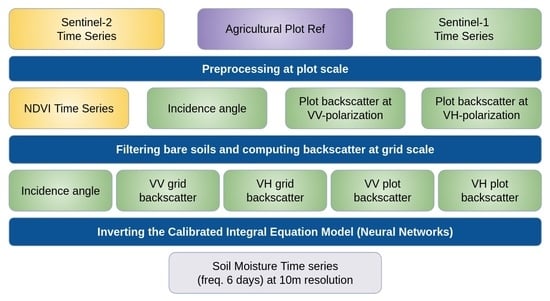
Our study builds upon the approach introduced by El Hajj et al. [16] and presents a fully autonomous solution based on Sentinel-1 (S1) images (without external data such as precipitation for example) to overcome the need for a priori weather information. In previous versions of the algorithm, weather data like precipitation and temperature were vital inputs used to guide the inversion algorithm in the estimation of soil moisture. The improved algorithm, proposed in this study, now relies on the average S1 radar signal, which is calculated on bare soil pixels and those with little vegetation within large areas of a few km${}^2$ each (10 km × 10 km grid cells). The hypothesis is inspired by the research of Bazzi et al. [20,21], establishing a strong correlation between the radar signal of bare or lightly vegetated soils and precipitation, with an increase in radar signal following heavy rainfall. Thus, a high signal corresponds to high soil moisture within the study area, which is mainly due to heavy rains. By utilizing the backscattering coefficients at the grid scale (a few km${}^2$), we can deduce the weather conditions used for the estimation domain partitioning without the need for a priori weather information. The second main objective is to study the potential of incorporating soil roughness estimates into the soil moisture estimation procedure, thereby analyzing the accuracy of surface soil moisture estimation when accounting for the influence of surface roughness on radar backscattering. The added value of using grid data and soil roughness estimates was studied in comparison to the previous models on the synthetic dataset generated by the calibrated IEM [13] and on a real dataset taken from two study sites where in situ soil moisture and soil roughness measurements are available.

2. Dataset Description and Problem Statement

In this section, we provide a detailed description of the two datasets used in our study. The first is the synthetic dataset obtained from the well-calibrated radar backscattering model IEM (Integral Equation Model). The second dataset is a real dataset obtained from field measurements conducted in Montpellier, France, and Kairouan, Tunisia. The performances of four neural network configurations using these two datasets are then compared in order to identify the strengths and limitations of each configuration.

2.1. Synthetic Dataset

The synthetic dataset is a collection of generated backscattering coefficients obtained from the calibrated IEM. The primary goal is to utilize a part of this dataset for training different machine learning configurations. The second part of this dataset will be used in the evaluation phase of our radar signal inversion approaches, providing a reliable benchmark for performance comparison.

2.1.1. Calibrated Radar Backscattering IEM

Recent studies showed that the calibrated IEM outperforms other well-known algorithms like Dubois, IEM, and Oh in terms of accurately reproducing radar signals [19,22,23,24]. As a result, this model was chosen for implementation in our study. For bare agricultural areas, the calibrated IEM calculates the backscattering coefficient ($\sigma$) by incorporating the sensor’s attributes (incidence angle, polarization, and radar wavelength) along with the soil’s parameters (soil moisture and soil roughness).

The radar backscattering coefficient for bare agricultural soil can be formulated as follows:

$$\sigma =IEM(\theta ,\lambda ,Pol,MV,HRMS)$$

(1)

where the sensor attributes are:

• $\sigma$ is the radar backscatter coefficient (no unit);
• $\theta$ is the incidence angle (°);
• $\lambda$ is the radar wavelength (cm);
• $Pol$ is the polarization (VV or VH; Sentinel-1 configuration).

The soil parameters:

• $MV$ is the soil moisture value (vol.%);
• $HRMS$ is the height root mean square of soil roughness (cm).

In our study, we estimate the soil moisture from the radar backscattering coefficients (single or dual polarization) and HRMS (measured or otherwise estimated). Thus, this inverse problem can be formulated as follows:

$$MV=IE{M}^{-1}(\sigma ,\theta ,HRMS)$$

(2)

In the case where the soil roughness is unknown, the inputs to the neural networks are the SAR data:

$$MV=IE{M}^{-1}(\sigma ,\theta )$$

(3)

Thus, inversion of the radar signal to estimate soil moisture does not necessarily require knowledge of the roughness. Inaccurate estimates of soil moisture would be obtained, however, in the case where the roughness value is unknown.

2.1.2. Range of Input Parameters

The input parameter values needed to build a relevant synthetic dataset were chosen to represent the same range of values as the parameters of real sensors and soils in agricultural areas. These inputs were used to generate backscattering coefficients using the calibrated IEM. The radar wavelength was set to 5.5 cm representing the Sentinel-1 radar wavelength. The incidence angle ($\theta$) ranged from 20° to 45° with a step size of 1°. For each incidence angle, soil roughness (HRMS) was considered from a generated list of values, ranging from 0.5 to 3.8 cm with a step size of 0.1 (34 values). For each ($\theta$, $HRMS$) combination, the soil moisture spanned from 4 to 40 vol.% with a step size of 2 vol.%.

Given that the SAR signal can show a strong increase with changes in soil moisture, especially after heavy rainfall [20], calculating the average radar signal over large areas (watershed or a given grid of several km²) using bare agricultural soils is useful, as it represents the general soil moisture conditions over the study area (very wet, wet to dry). In this study, as input to our soil moisture estimation algorithm, we use information at the plot level (marked with a “p”, VVp and VHp) and information at the grid level (marked with a “g”, VVg and VHg). For grid synthetic data, we followed the following scheme: We start by fixing the grid soil moisture MVg between 4 and 40 vol.%. Next, for a given MVg value and each combination of incidence angle and soil roughness within the chosen ranges, 100 samples of soil moisture at plot scale were generated using a bounded normal distribution with a mean value equal to the soil moisture at grid scale and a standard deviation of 10 vol.%. The generated MVp samples were constrained within the range [MVg − 10, MVg + 10], and the soil moisture at the plot scale was filtered to retain only those between 4 and 40 vol.%. Thus, in addition to MVp values, we can also have MVg values as input in our inversion algorithm.

2.1.3. Synthetic Dataset Generation

Once the synthetic inputs are generated, we run the calibrated IEM to generate the backscatter coefficients for the grid level using the grid soil moisture values (${\sigma }_{V{V}_g}$, ${\sigma }_{V{H}_g}$) or for the plot level using the soil moisture at plot scale (${\sigma }_{V{V}_p}$, ${\sigma }_{V{H}_p}$). Then, an absolute error corresponding to the SAR observation accuracy was added to the simulated backscattering coefficients to obtain a more realistic synthetic dataset. For Sentinel-1, this error is defined by the absolute radiometric accuracy, which is equal to 0.70 dB and 1.0 dB for VV and VH polarizations, respectively [10]. Accordingly, for each element of our dataset, five noise samples were randomly selected from the zero-mean Gaussian noise distribution with a standard deviation of 0.7 and 1.0 dB, respectively, for VV and VH. The randomly selected noise values were then added to the IEM’s simulated $\sigma$ at both scales (plot and grid). Finally, our noisy synthetic dataset, in VV and VH polarizations, is composed of about 8 million elements.

Table 1. Example of synthetic data generated by the calibrated IEM using Sentinel-1 wavelength.

IEM Inputs				IEM Outputs
$\theta$	HRMS	MVg	MVp	${\sigma }_{{\mathit{VV}}_{\mathit{p}}}$	${\sigma }_{{\mathit{VH}}_{\mathit{p}}}$	${\sigma }_{{\mathit{VV}}_{\mathit{g}}}$	${\sigma }_{{\mathit{VH}}_{\mathit{g}}}$
20.0	0.5	4.0	6.56	−12.16	−27.58	−9.30	−21.21
20.0	0.5	4.0	6.45	−10.72	−24.56	−9.06	−19.27
20.0	0.5	4.0	10.76	−10.21	−24.82	−8.77	−20.32
…	…	…	…	…	…	…	…
45.0	3.8	40.0	36.98	−6.04	−15.49	−7.67	−17.01
45.0	3.8	40.0	32.38	−6.36	−17.66	−8.60	−17.55
45.0	3.8	40.0	38.40	−4.78	−15.53	−6.40	−17.39

shows an example of the possible combinations of our input parameters in an eight-column data format. Each row represents a unique data combination defined by a given radar incidence angle ($\theta$), surface roughness, and soil moisture at plot and grid scales. ${\sigma }_{V{V}_p}$ and ${\sigma }_{V{H}_p}$ were simulated using ($\theta$, $HRMS$, $MVp$), while ${\sigma }_{V{V}_g}$ and ${\sigma }_{V{H}_g}$ were simulated using ($\theta$, $HRMS$, $MVg$).

In this study, half of the synthetic dataset is used for training the neural networks, and the other half is used for their evaluation; the evaluation half is referred to as the validation dataset.

2.2. Real Dataset

In this part, we introduce our real dataset from two distinct study areas in Montpellier, France, and Kairouan, Tunisia. This dataset offers diverse environmental conditions with associated satellite data and field measurements. The satellite data contain the backscatter coefficients in VV and VH polarizations calculated from Sentinel-1 ascending orbit images. In addition, field measurements provide measured soil moisture (MVp) and surface roughness (HRMS) collected at reference fields. The proposed machine learning configurations for soil moisture estimations are evaluated using the in situ measured soil moisture in the two study sites.

2.2.1. Montpellier Dataset

Study Area

The first real dataset is collected in a study site located in the Occitanie region of France as shown in Figure 1. Figure 1 illustrates the delineated parcels within the study area following the application of a Normalized Difference Vegetation Index (NDVI) threshold filter of less than 0.4. Utilizing Sentinel-2 (S2) images, NDVI values were calculated for each individual parcel across the entire timeline of our research period. Subsequently, Figure 1 shows only the parcels possessing for at least one date an NDVI value less than 0.4. With a relatively flat terrain topography, the study area is composed mainly of forest, vineyards, grasslands, and agricultural fields (mainly wheat). The climate of the study site is Mediterranean with a rainy season between mid-October and March and an average annual cumulative rainfall of approximately 750 mm. The average air temperature varies between 2.9 and 29.3 °C. The topsoil texture of the agricultural fields is loam.

Sentinel-1 Images

Over the French study site, 28 Sentinel-1 images (S1) acquired between 15 April 2016 and 26 June 2018 were used. The Sentinel-1 (S1) images are downloadable from the Copernicus website (https://scihub.copernicus.eu/dhus/#/home, accessed on 1 November 2022). The 28 S1 ascending orbit images used were acquired in IW imaging mode with the VV and VH polarizations. The S1 images were calibrated using the S1 toolbox developed by the ESA (European Spatial Agency). The calibration aims to convert the digital number values of S1 images into backscattering coefficients ($\sigma$) in a linear unit. Thus, for each polarization, the average signal of all pixels in each plot is computed to obtain a single representative value for each reference plot (${\sigma }_p$). Then, to build real SAR signals at grid scale (${\sigma }_g$), for each S1 acquisition and polarization, the average backscatter coefficient is computed using all agricultural pixels with low NDVI values (below 0.4).

Sentinel-2 Images

All available Sentinel-2 (S2) optical images over each study site/year were downloaded from the Theia website (https://www.theia-land.fr/, accessed on 1 November 2022). S2 images cover the same time span of the S1 acquisitions for each site/year. Cloud-free optical images are available at a frequency of approximately two images per month. The S2 images provided by Theia are corrected for atmospheric interference and thus are called Level-2A products. S2 images were mainly used to calculate the NDVI time series for each reference field.

In Situ Measurements

In situ measurements of soil moisture and surface roughness were collected during 28 field surveys between 15 April 2016 and 26 June 2018. These fields correspond to bare or partially vegetated soils (NDVI lower than 0.4). Soil moisture at plot scale (MVp) was measured within a window of 2 h with respect to the Sentinel-1 acquisition date. For each reference plot, 20 to 30 measurements of volumetric soil moisture were conducted in the top 5 cm of soil by means of a calibrated TDR (Time Domain Reflectometry) probe. The study utilizes ML2x model theta probes from ThetaProbe, dealing with the challenges associated with TDR moisture measurement quality quantification. In line with the findings of Walker et al. [25], it has been confirmed that TDR measurements, especially when facilitated by 10 and 15 cm waveguides, align closely with gravimetric results, delivering an accuracy of around ± 2.5 vol.%.

All soil moisture measurements within each plot were averaged to provide a mean value for each plot. The range of the soil moisture value is between 4.5 and 32.5 vol.%. In addition, the soil roughness parameter HRMS was determined using a needle profilometer with a length of 1 m and a needle spacing of 1 cm. For each reference plot, five parallel roughness profiles along the SAR line of sight were recorded, and another five were perpendicular to the line. Thus, by processing the roughness profile, the HRMS was derived. In our study, the recorded HRMS values of the reference plots varied between 0.5 and 4.0 cm. It is important to note that the parcels are not irrigated.

Finally, our French dataset is composed of 198 elements with radar backscattering coefficients (in VV and VH) and in situ measurements of soil moisture (MVp) and surface roughness (HRMS). Each element of this real dataset represents a reference plot with an associated MVp value, incidence angle and mean backscattering coefficients in VV and VH. The incidence angles of our reference plots vary from 39° to 41°. This dataset was only used to validate our soil moisture estimates.

2.2.2. Kairouan Dataset

Study Area

The second real dataset was collected over a study area located in the Kairouan Governorate of Tunisia, as shown in Figure 2, in central Tunisia. The climate in this region is semi-arid, with an average annual rainfall of approximately 300 mm/year, characterized by a rainy season lasting from October to May, with the two rainiest months being October and March. The mean temperature in Kairouan City is 19.2 °C (minimum of 10.7 °C in January and maximum of 38.6 °C in August). The landscape is mainly flat, and the vegetation is dominated by agricultural production (cereals, olive groves, fruit trees, market gardens, and bare soils).

Sentinel-1 Images

A total of 17 Sentinel-1 images were acquired between 6 December 2015 and 30 March 2017 over this study area in ascending mode. The same processing of S1 images was performed as that for the Montpellier study site.

Sentinel-2 Images

The same processing of S2 images was performed as that for the Montpellier study site.

In Situ Measurements

Ground campaigns were carried out at the same time as the 17 Sentinel-1 acquisitions. The ground measurements made on the reference fields involved the characterization of the soil moisture using a theta-probe instrument. On average, 35 bare soil reference fields were selected at each Sentinel-1 visit. For each reference field, approximately 20 handheld theta-probe measurements were made at a depth of 5 cm. The samples were taken from various locations in each reference field within a two-hour time frame between 15:40 and 17:40, coinciding with the time of each S1 acquisition. The volumetric moisture ranged between 4.0 and 32.0 vol.%. Soil roughness measurements were not available for the Kairouan dataset as opposed to the Montpellier dataset. It is important to note that the Kairouan parcels are frequently irrigated. Finally, our Tunisian dataset is composed of 201 elements with radar backscattering coefficients (in VV and VH) and in situ measurements of soil moisture (MVp). The incidence angles of our reference plots vary from 39.5° to 39.9°. This dataset was only used to validate our soil moisture estimates.

In summary, the synthetic dataset will serve as a benchmark for training and evaluating various machine learning configurations through a wide range of backscattering coefficients obtained from the calibrated IEM. Additionally, the real dataset offers a comprehensive and diverse set of environmental conditions, satellite data, and field measurements from two distinct study areas in Montpellier, France, and Kairouan, Tunisia. By comparing the soil moisture estimated from the sensor attributes and the in situ soil moisture, our study can evaluate the machine learning configurations on veritable data. The field measurements obtained from both study areas provide us with real data on soil attributes, enabling us to ensure that the satellite data analysis is grounded in reality and is providing an accurate representation of the soil attributes being studied.

3. Methodology

In this section, we introduce our experimental setups for inverting Sentinel-1 signals in order to estimate soil moisture. First, inversion models are described. Then, the model architecture and the process of model training and optimization are presented. Finally, the different input/output configurations of the inversion model as well as the precision metrics used for the models evaluation are detailed.

3.1. Inversion Algorithm

This study focuses on estimating soil moisture content using radar backscattering coefficients as input data (inverse Equations (2) and (3)). Therefore, the problem is formulated as developing a model that can effectively estimate soil moisture levels based on the provided radar backscattering coefficients, enabling a better understanding and monitoring of soil moisture dynamics. In fact, the inversion model uses the neural network technique trained on the synthetic dataset described in the previous section in order to inverse the radar signal. The trained neural networks are then used to estimate soil moisture using the real backscatter computed from Sentinel-1 images.

Given an input vector of S1 radar measurements, we want to learn the function $\mathcal{N}$ that maps the radar measurements to soil moisture values MV. This problem can be formulated as:

$$MV=\mathcal{N}(\sigma ,\theta ,HRMS;w)+ϵ$$

(4)

where the the inputs are $\sigma$—the radar backscatter coefficient (dB) at VV and VH polarizations (Sentinel-1 configuration) provided by the satellite images and spatially averaged at plot (VVp and VHp) or grid scales (VVg and VHg), $\theta$—the associated incidence angle (°), and $HRMS$—the soil roughness value (if available). In the vector $w=\left(w,b\right)$, w denotes the weights and b denotes the bias of the neural network $\mathcal{N}$. $ϵ$ denotes the estimation error. One of the objectives of this study is to find the best attribute configuration with the minimum $ϵ$.

The adopted neural network architecture is composed of two hidden layers. The first layer is associated with a linear activation function, while the second hidden layer uses a tangent sigmoid activation function. Both hidden layers contain 20 neurons each [16]. In fact, after comparing this neural network with other machine learning models (gradient-boosted decision tree and multi-layer perceptron), we found that the added value of changing the machine learning model can be ignored in relation to the added value of changing the machine learning model’s attributes. Let $W_1, W_2,$ and $W_3$ be the weight matrices of dimensions $20\times n, 20\times 20,$ and $1\times 20$, respectively, and let $b_1, b_2,$ and $b_3$ be the bias vectors of dimensions $20\times 1, 20\times 1,$ and $1\times 1$, respectively. For the first hidden layer, we use a linear transfer function, which is denoted as $g_1(·)$. For the second hidden layer, we use a tangent sigmoid transfer function, which is denoted as $g_2(·)$, and for the last layer, we use the identity function, which is denoted as $h(·)$. The forward pass can be formulated as:

(a)

First hidden layer (linear transfer function):

$$z_1=W_{1}x+b_1,a_1=g_1\left(z_1\right),a_1=z_1$$

(5)

(b)

Second hidden layer (tangent sigmoid transfer function):

$$z_2=W_2{a}_1+b_2,a_2=g_2\left(z_2\right),a_2=tanh\left(z_2\right)$$

(6)

(c)

Output layer:

$$z_3=W_3{a}_2+b_3,\widehat{y}=h\left(z_3\right)$$

(7)

where x is the input vector containing the sensor attributes values and $\widehat{y}$ is the estimated output.

The optimization problem aims to minimize a loss function $L(\widehat{y},y)$, where $\widehat{y}$ is the estimated output and y is the observed output. We want to find the optimal weight matrices $(W_1,W_2,W_3)$ and bias vectors $(b_1,b_2,b_3)$ that minimize the loss function:

$$w^{*}=arg\underset{w}{min}L(\widehat{y},y)$$

(8)

with $w=(W_1,W_2,W_3,b_1,b_2,b_3)$.

This is typically achieved through an iterative process such as gradient descent, which updates the weights and biases based on the gradients of the loss function with respect to the model parameters. In our case the optimization technique used is the Levenberg–Marquardt (LM) algorithm [26] (see Appendix A). The Levenberg–Marquardt (LM) algorithm is a popular optimization technique that combines the features of gradient descent and the Gauss–Newton method, making it particularly suitable for solving nonlinear least-squares problems (see Appendix A). The LM algorithm is applied to our neural networks ($\mathcal{N}$) for training by minimizing the sum of squared errors (SSE) loss function. The Levenberg–Marquardt algorithm is an optimization algorithm that does not require a learning step but uses instead an adaptive damping factor, which has a default value of 1. This quasi-Newton optimization approach assumes that the function being optimized can be locally approximated by a second-order Taylor series. The process generally begins with an initial guess, employs the Jacobian matrix to determine the steepest descent direction, and utilizes the Hessian matrix to calculate the descent step to the next point. This process continues until there is no improvement in the loss value by at least ${10}^{-4}$.

3.2. Evaluated Sentinel-1 Configurations

Various configurations aimed at optimizing soil moisture estimation accuracy were evaluated. These configurations involve the integration of Sentinel-1 polarizations, partitioning the estimation domain into dry and wet conditions, incorporating a Sentinel-1 large-scale signal thanks to the grid backscatter coefficients, and training neural networks with soil roughness estimates.

• Configuration 1: Analyze the effect of Sentinel-1 polarizations

Three inversion Sentinel-1 configurations were tested: (1) VV polarization alone; (2) VH polarization alone; and (3) both VV and VH polarizations. In this configuration, the soil roughness parameter HRMS is ignored. They can be formulated as:

$$\begin{array}{c}Config\_1\_VV:MVp=\mathcal{N}({\sigma }_{V{V}_p},\theta ;w)+ϵ\\ Config\_1\_VH:MVp=\mathcal{N}({\sigma }_{V{H}_p},\theta ;w)+ϵ\\ Config\_1\_VV\_VH:MVp=\mathcal{N}({\sigma }_{V{V}_p},{\sigma }_{V{H}_p},\theta ;w)+ϵ\end{array}$$

(9)

• Configuration 2: Separate the MVp estimation domain into two separate domains: one for dry to slightly wet and one for very wet

Using the same polarizations as in the previous configuration, we separate our MVp solution search domain into two domains: one with a search for a solution for dry to slightly wet soil conditions and one for a solution for wet to very wet soil conditions. This configuration needs a priori information on MVp (a priori dry to slightly wet or very wet). Partitioning the estimation domain into distinct dry and wet conditions and training dedicated neural networks for each domain may significantly enhance soil moisture estimation accuracy [16]. By focusing on domain-specific patterns and relationships, the specialized neural networks can capture the complexities associated with soil moisture variations more effectively. In the case of a priori dry to slightly wet soil, $\mathcal{N}$ will be built up using the synthetic training dataset elements with MVp between 4 and 30 vol.%. Contrarily, in the case of a priori very wet soil conditions, $\mathcal{N}$ will be developed using the synthetic training dataset elements with MVp between 20 and 40 vol.%. An overlap of 10 vol.% on MVp is considered between the dry to slightly wet and the very wet training datasets of $\mathcal{N}$. During the evaluation, the dry $\mathcal{N}$ is applied on attributes with MVp < 25, while the wet $\mathcal{N}$ is applied on attributes with MVp ≥ 25. The 25 vol.% moisture threshold is the midpoint between the two moisture ranges applied to the neural network for dry/wet and very wet conditions. Both this midpoint value and the selected ranges are grounded in field observations where soils are usually very wet following substantial rainfall, typically recording humidity between 25 and 40 vol.%. The dry to wet conditions correspond to soil after an absence of precipitation (dry for the summer following a prolonged lack of rain and wet generally in the autumn or winter after a relatively short duration without rain). In an operational context, the choice between ${\mathcal{N}}_{dry}$ or ${\mathcal{N}}_{wet}$ is determined by meteorological data, primarily focusing on precipitation. For example, if there has been significant rainfall one or two days before the S1 acquisition, the ${\mathcal{N}}_{wet}$ would be used; otherwise, the ${\mathcal{N}}_{dry}$ is applied. In this configuration, the soil roughness parameter HRMS is ignored.

This is formulated as:

$$\begin{array}{c}Config\_2\_VV:MV{p}_{dry}={\mathcal{N}}_{dry}({\sigma }_{V{V}_p},\theta ;w)+{ϵ}_{dry}\\ MV{p}_{wet}={\mathcal{N}}_{wet}({\sigma }_{V{V}_p},\theta ;w)+{ϵ}_{wet}\\ Config\_2\_VH:MV{p}_{dry}={\mathcal{N}}_{dry}({\sigma }_{V{H}_p},\theta ;w)+{ϵ}_{dry}\\ MV{p}_{wet}={\mathcal{N}}_{wet}({\sigma }_{V{H}_p},\theta ;w)+{ϵ}_{wet}\\ Config\_2\_VV\_VH:MV{p}_{dry}={\mathcal{N}}_{dry}({\sigma }_{V{V}_p},{\sigma }_{V{H}_p},\theta ;w)+{ϵ}_{dry}\\ MV{p}_{wet}={\mathcal{N}}_{wet}({\sigma }_{V{V}_p},{\sigma }_{V{H}_p},\theta ;w)+{ϵ}_{wet}\end{array}$$

(10)

• Configuration 3: Assess the added value of using the grid information in addition to plot scale

In this configuration, we hypothesize that incorporating backscatter coefficients at the grid scale into the soil moisture estimation process, in addition to backscatter coefficients at the plot scale, can improve the accuracy of MVp estimation, potentially offering an alternative to the domain-separated approach which necessitates weather data for selecting the appropriate neural network (dry to slightly wet or very wet). This hypothesis assumes that integrating grid coefficients can inform $\mathcal{N}$ about the soil moisture status in the study area, enabling the inversion model to adapt to both dry and wet soil characteristics. We also chose to use both polarizations as its the most precise configurations. There are two subcases of configuration 3, which are formulated as:

$$\begin{array}{c}Config\_3\_grid:MVp={\mathcal{N}}_{MVp}({\sigma }_{V{V}_p},{\sigma }_{V{H}_p},{\sigma }_{V{V}_g},{\sigma }_{V{H}_g},\theta ;w)+{ϵ}_{MVp}\\ Config\_3\_grid\_MVg:M{V}_g={\mathcal{N}}_{MVg}({\sigma }_{V{V}_g},{\sigma }_{V{H}_g},\theta ;w)+{ϵ}_{MVg}\\ MV{p}_{dry}={\mathcal{N}}_{dry}({\sigma }_{V{V}_p},{\sigma }_{V{H}_p},{\sigma }_{V{V}_g},{\sigma }_{V{H}_g},\theta ;w)+{ϵ}_{dry}\\ MV{p}_{wet}={\mathcal{N}}_{wet}({\sigma }_{V{V}_p},{\sigma }_{V{H}_p},{\sigma }_{V{V}_g},{\sigma }_{V{H}_g},\theta ;w)+{ϵ}_{wet}\end{array}$$

(11)

Equation (11) gives a detailed presentation of the neural networks and their inputs used in configuration 3. In $Config\_3\_grid$ only ${\mathcal{N}}_{MVp}$ was used; this network was trained using the backscatter coefficients for VV and VH polarizations on the grid and plot scales. In $Config\_3\_grid\_MVg$, three $\mathcal{N}$ were used: ${\mathcal{N}}_{MVg}$ is trained to estimate $MVg$ using the backscatter coefficients for VV and VH on the grid scale, and the $MVg$ value estimated from ${\mathcal{N}}_{MVg}$ will serve as a dry/wet domain separator. If the estimated $MVg<25$ vol.%, the config will use ${\mathcal{N}}_{dry}$ in order to estimate $MVp$; otherwise, it will use ${\mathcal{N}}_{wet}$. The second and third $\mathcal{N}$ values were trained using the backscatter coefficients for VV and VH polarizations on the grid and plot scales: ${\mathcal{N}}_{dry}$ uses backscatter coefficients on $MVp<30$ vol.% and ${\mathcal{N}}_{wet}$ uses backscatter coefficients on $MVp>20$ vol.%. In this configuration, the soil roughness parameter HRMS is ignored.

• Configuration 4: Analyze the added value of using soil roughness estimates

In this last configuration, we hypothesize that training neural networks with soil roughness estimates, in conjunction with incorporating grid backscatter coefficients and partitioning estimation domains, can potentially improve soil moisture estimation accuracy. This hypothesis suggests that by accounting for the complex relationships between soil moisture, surface roughness, and backscatter signals, neural networks can better capture the intricacies of soil moisture variations across various surface conditions. There are two subcases of configuration 4, which are formulated as:

$$\begin{array}{c}Config\_4\_grid:HRMS={\mathcal{N}}_{HRMS}({\sigma }_{V{V}_p},{\sigma }_{V{H}_p},{\sigma }_{V{V}_g},{\sigma }_{V{H}_g},\theta ;w)+{ϵ}_{HRMS}\\ MVp={\mathcal{N}}_{MVp}({\sigma }_{V{V}_p},{\sigma }_{V{H}_p},{\sigma }_{V{V}_g},{\sigma }_{V{H}_g},HRMS,\theta ;w)+{ϵ}_{MVp}\\ Config\_4\_grid\_MVg:M{V}_g={\mathcal{N}}_{MVg}({\sigma }_{V{V}_g},{\sigma }_{V{H}_g},\theta ;w)+{ϵ}_{MVg}\\ HRM{S}_{dry}={\mathcal{N}}_{HRM{S}_{dry}}({\sigma }_{V{V}_p},{\sigma }_{V{H}_p},{\sigma }_{V{V}_g},{\sigma }_{V{H}_g},\theta ;w)+{ϵ}_{HRM{S}_{dry}}\\ HRM{S}_{wet}={\mathcal{N}}_{HRM{S}_{wet}}({\sigma }_{V{V}_p},{\sigma }_{V{H}_p},{\sigma }_{V{V}_g},{\sigma }_{V{H}_g},\theta ;w)+{ϵ}_{HRM{S}_{wet}}\\ MV{p}_{dry}={\mathcal{N}}_{dry}({\sigma }_{V{V}_p},{\sigma }_{V{H}_p},{\sigma }_{V{V}_g},{\sigma }_{V{H}_g},HRM{S}_{dry},\theta ;w)+{ϵ}_{dry}\\ MV{p}_{wet}={\mathcal{N}}_{wet}({\sigma }_{V{V}_p},{\sigma }_{V{H}_p},{\sigma }_{V{V}_g},{\sigma }_{V{H}_g},HRM{S}_{wet},\theta ;w)+{ϵ}_{wet}\end{array}$$

(12)

In $Config\_4\_grid$ two $\mathcal{N}$ values were used. ${\mathcal{N}}_{HRMS}$ was trained to estimate the soil roughness using the backscatter coefficients for VV and VH polarizations on the grid and plot scales, while ${\mathcal{N}}_{MVp}$ was trained to estimate the soil moisture using the backscatter coefficients for VV and VH polarizations on the grid and plot scales in addition to soil roughness. Furthermore, to account for the uncertainties on HRMS estimated from SAR images [7] in the training phase, a zero-mean Gaussian noise was added to HRMS with a standard deviation of 0.5. The estimated $HRMS$ value from ${\mathcal{N}}_{HRMS}$ is used to estimates $MVp$.

In $Config\_4\_grid\_MVg$, five $\mathcal{N}$ were used; like in $Config\_3\_grid\_MVg$, ${\mathcal{N}}_{MVg}$ is used to separate the estimation domain of $HRMS$ and $MVp$ into two domains: dry–wet/very wet using the same thresholds on $MVg$ as $Config\_3$. Then, $HRMS$ is estimated according to dry or wet conditions (${\mathcal{N}}_{HRM{S}_{dry}}$ or ${\mathcal{N}}_{HRM{S}_{wet}}$), and then, this estimate of HRMS is used in the network to estimate MVp (${\mathcal{N}}_{dry}$ or ${\mathcal{N}}_{wet}$).

Note that configurations 1 and 2 have already been tested by El Hajj et al. [16] and that in our study, they serve as benchmarks for configurations 3 and 4.

3.3. Evaluation Metrics

The first evaluation metric used is the root mean squared error (RMSE). RMSE is a valuable metric in soil moisture estimation due to its comprehensive assessment of accuracy, emphasis on larger errors, and clear interpretability. Its consideration of larger discrepancies ensures significant errors are addressed. It can be formulated as:

$$\mathrm{RMSE}=\sqrt{\frac{1}{N}\sum _{i=1}^N{(y_i-{\widehat{y}}_i)}^2}$$

(13)

with N representing the number of data, $y_i$ denoting the observed value for the i-th data point, and ${\widehat{y}}_i$ denoting the estimated value for the i-th data point.

The second evaluation metric used is bias. The bias metric serves as an important evaluation tool due to its interpretability and ability to quantify systematic error. By measuring the average difference between estimated and observed values, the bias metric offers valuable insights into the model’s overall performance. This metric enables us to identify and understand the extent to which a model consistently overestimates or underestimates the target variable:

$$\mathrm{Bias}=\frac{1}{N}\sum _{i=1}^N({\widehat{y}}_i-y_i)$$

(14)

The third evaluation metric used is the mean absolute percentage error (MAPE). MAPE is an essential evaluation metric that provides a clear understanding of a model’s prediction accuracy in terms of relative error. It computes the average percentage differences between estimated and observed values:

$$\mathrm{MAPE}=\frac{1}{N}\sum _{i=1}^N\left|\frac{y_i-{\widehat{y}}_i}{y_i}\right|$$

(15)

4. Result Analysis

In this section, the effectiveness of the configurations described in the Methodology section will be compared on both the synthetic validation set (half the dataset that was not used for training) and the real dataset. This comprehensive evaluation will allow us to assess the performance of each configuration under controlled and real-world conditions, thereby providing a better understanding of their applicability and potential limitations. By examining the outcomes of these configurations, we aim to determine the most effective configurations for optimizing soil moisture estimation accuracy.

4.1. Using Synthetic Validation Set

All the configurations previously discussed are ranked using the three mentioned metrics and displayed as a bar plot leaderboard in Figure 3. For configuration 1, which focused on the effect of Sentinel-1 polarization, the combined use of VV and VH polarizations yielded a more accurate estimation compared to using either polarization individually with an RMSE decrease of about 0.7 vol.% for VH and 0.35 vol.% for VV, as shown in Figure 3. In configuration 2 (with a priori information on MVp), which involved separating the estimation domain into dry and wet conditions using a weather forecasting framework, improved accuracy was observed in comparison to configuration 1, particularly when both VV and VH polarizations were utilized, with an RMSE decrease of 0.4 vol.%. For configuration 3, which assessed the added value of using the radar signal computed at the grid scale, the two subcases (Config_3_grid and Config_3_grid_MVg) show that directly estimating MVp with grid information produces the same performance as estimating MVg and then partitioning the MVp to dry and wet using the estimated MVg. However, the three precision metrics show a clear improvement in $MVp$ accuracy using the grid-scale information compared to configurations 1 and 2 except for configuration 2 when both polarizations are used, where we obtain an RMSE that improves only of about 0.2 vol.%. Lastly, in configuration 4, which analyzed the added value of using soil roughness estimates, the integration of soil roughness estimates did not improve the $MVp$ estimation accuracy in comparison to configuration 3. Figure 3 shows that we obtain the same order of magnitude on all three precision metrics between configurations 3 and 4: about 3.5 vol.% on RMSE and 14% on MAPE.

Thus, the evaluation of these configurations suggests that the combined use of VV and VH polarizations, separating the MVp estimation domain into dry and wet conditions yields better results than the configuration without a priori information on MVp (configuration 1). The incorporation of a radar signal computed at grid scale using the bare agricultural soils included in each grid cell replaces the priori information on the soil moisture conditions, which were extracted in general using expert knowledge from meteorological data [16]. The added value of soil roughness estimates is negligible compared to other configurations without the use of roughness information.

4.1.1. Performance of Used $\mathcal{N}$ as a Function of the Soil Moisture

In this part, model sensitivities to soil moisture are analyzed on the synthetic validation set. Figure 4 shows the three precision metrics (Bias, RMSE and MAPE) calculated for intervals of soil moisture values as boxplots. In configurations 1 and 2, the percentile values reveal a general increase in RMSE values as the MVp level increases. The RMSE passes of about 2 vol.% for MVp in the range 4 to 7.5 vol.% to about 5 vol.% for MVp in the range 37.5 to 40 vol.%, indicating a decline in soil moisture estimation accuracy as the soil moisture levels increase, as shown in Figure 4. Many studies have shown that the radar signal increases with soil moisture for SM values ranging between 5 vol.% and approximately 30 vol.% (e.g., [5]). In Baghdadi et al. [27], the behavior of radar signals as a function of SM under very wet soil conditions (SM > 30 vol.%) was analyzed. The results showed that under conditions of high moisture (SM between 27 and 41 vol.%), the radar signal is stable when SM ranges between 27 and 32 vol.%, and that it decreases beyond this threshold. The latter declines by about 4 dB, when SM increases from 32 to 41 vol.%. As the radar signal begins to decrease with soil moisture when the moisture is above approximately 30 vol.%, an accurate estimation of moisture becomes impossible. For instance, the radar signal for a soil at about 40 vol.% is of the same order of magnitude as that for a soil with a moisture of 25 vol.%. However, the MAPE shows that despite the increase in the RMSE, the performance of the soil moisture estimations is improved as the soil moisture level increases. For example, the MAPE for the level [32.5, 37.5[ was about 10% less than that for low soil moisture values between 4 vol% and 7.5 vol%. This suggests that the soil moisture estimation accuracy is influenced by the soil moisture levels. In configurations 3 and 4, without a priori information on MVp in order to estimate the soil moisture, the percentile values demonstrate an improvement in soil moisture estimation accuracy compared to configurations 1 and 2. In fact, for seven of the eight MVp ranges, the difference between the 25% and 75% percentiles is smaller for configurations 3 and 4 than for configurations 1 and 2 on all metrics, showing that not only configurations 3 and 4 are more precise but also more stable. Finally, in configuration 4, where the estimated HRMS is used to optimize the MVp estimates, the percentile values reveal a very slight improvement in soil moisture estimation accuracy compared with the other configurations. The bias metric shows that all configurations tend to overestimate soil moisture for MVp under 32.5 vol.% and start to underestimate soil moisture values above 32.5 vol.%.

4.1.2. Performance of Used $\mathcal{N}$ as a Function of the Soil Roughness Value

In this section, we evaluate how the best subcase of each configuration reacts to soil roughness variations on the synthetic validation dataset. The precision metrics computed over diverse soil roughness ranges are presented as boxplots in Figure 5. For all configurations, the percentile values show high RMSE and MAPE values for low (HRMS < 1.5 cm) and high soil roughnesses (HRMS ≥ 2.5 cm); they also show the lowest scores for HRMS range between 1.5 and 2.5 cm Figure 5. The bias shows that all configurations tend to underestimate MVp for low roughnesses (HRMS < 1.5 cm) and overestimate MVp for high roughnesses (HRMS ≥ 2.5); this suggests that the soil moisture estimation accuracy is influenced by soil roughness and that the best HRMS range for estimating MVp is between 1.5 and 2.5 cm, as shown in Figure 5. In configurations 3 and 4 without a priori information on MVp, the percentile values demonstrate an improvement in soil moisture estimation accuracy compared to configurations 1 and 2, especially for HRMS ≥ 1.5. Finally, in configuration 4, the percentile values reveal a slightly greater improvement in soil moisture estimation accuracy than in other configurations, thus affirming that $\mathcal{N}$ might benefit from training using soil roughness estimates.

4.2. Using Real Dataset

In this section, we present the results of our evaluation on the real dataset, which originates from the Kairouan region in Tunisia and the Occitanie region in France. The bar chart, referenced in Figure 6, displays the rankings for the previously discussed configurations, using data from the real dataset. The results of configurations 1 and 2 align with our findings from the synthetic dataset, where the combination of both polarizations significantly improves estimation accuracy compared to using each polarization individually (Figure 6). The use of both polarization reduces the RMSE on MVp estimates of about 0.5 vol.% in the case of configuration 1 and of about 0.35 vol.% for configuration 2. In addition, the use of two polarizations considerably reduces bias, as shown in Figure 6. The results of configuration 3 suggest that incorporating grid information optimizes soil moisture estimation accuracy compared to the first configuration. Also, the accuracy analysis on the MVp estimates obtained by configuration 3 shows slightly better accuracy gain compared to configuration 2, confirming that we can achieve higher accuracy using grid information without the need for a priori weather. The integration of roughness estimates (configuration 4) shows a relatively minor improvement in soil moisture estimates compared to configurations 2 and 3. These results are consistent with the synthetic dataset results.

4.2.1. Performance of Used $\mathcal{N}$ as a Function of the Soil Moisture

In this part, model sensitivities to soil moisture are analyzed on real data. Figure 7 presents bias, RMSE and MAPE scores as percentile values for our better configurations (conf_1_VV_VH, conf_2_VV_VH, conf_3_grid_MVg, and conf_4_grid) across various soil moisture levels ranging from very dry to very wet conditions. For all configurations, the percentile values reveal a general decrease in RMSE and MAPE values as the MVp increases in the MVp range lower than 17.5 vol.% (from very dry to slightly wet soils). Then, we observe a change in trend as the MVp level increases from 17.5 vol.% (slightly wet) to 32.5 (wet), as shown in Figure 7. Furthermore, the bias percentile values show that our model is prone to a slight overestimation in dry soil conditions and high underestimation in wet soil conditions (bias reaches 10 vol.% for MVp higher than 32.5 vol.%). Separately, Figure 7 shows that configurations 3 and 4 give better scores from very dry to wet conditions (best overall percentiles on all scores) and that configuration 1 gives the best scores on very wet conditions.

4.2.2. Performance of Used $\mathcal{N}$ as a Function of the Soil Roughness

This part focuses on examining the sensitivities of the model to soil roughness using real data. Figure 8 displays percentile values of bias, RMSE, and MAPE scores for the best four configurations across different soil moisture levels. Soil moisture estimates appear to be unaffected by variations in soil roughness, since the bias metric demonstrates relatively balanced bias scores across all soil roughness ranges, as shown in Figure 8. This observation holds true for every configuration tested. Consequently, soil roughness does not introduce any significant bias into soil moisture assessment. The dependence between the accuracy on the estimation of MVp and the soil roughness is less well marked with the real data because only a few measurements have roughnesses lower than 1 cm or higher than 3 cm. Indeed, it is only on the small and strong roughnesses that we could observe a strong dependence on the radar signal in the C-band [28].

5. Discussion

In this part, we discuss the limitations of our S1 signal inversion procedures. The first limitation concerns the accuracy of our model results, which may be due to an incorrect choice to use a dry network instead of a wet network (configurations 2, 3, and 4). This issue arises in cases where some fields are irrigated, such as in the Kairouan study site. Indeed, for an irrigated site, the moisture of a plot can be very low (if not irrigated) or very high (if the plot is irrigated), while the radar signal at the grid scale is probably low if only a few plots are irrigated or very high if most of the plots are irrigated at a very close time (this is unlikely). Thus, the soil moisture of recently irrigated plots could be underestimated during the summer. The dry NN will be used during this time of year even if some plots are irrigated because most of the other plots are not irrigated (MVg is generally lower than 20 vol.%). This underestimation will occur since the dry NN will have difficulty estimating moisture above 20 vol.%. Figure 9 shows this underestimation of soil moisture for recently irrigated plots in the Kairouan study site, while the dry NN performs well for plots with moisture lower than 20 vol.%.

For agricultural soil, the backscattered radar signal is heavily influenced by factors such as soil roughness, dielectric properties (including moisture content and soil composition), and characteristics of the vegetation (such as biomass, vegetation water content, and geometry of vegetation elements). Following a rainfall or irrigation event, the soil moisture eventually increases, which corresponds to an increase in the radar signal. Irrigation not only alters soil moisture but also the surface roughness, as it generally leads to a slight decrease in soil roughness. However, the effect of irrigation on roughness is typically not taken into account because (1) this slight decrease in roughness is challenging to measure, and (2) this minor decrease in roughness will have a significantly smaller effect on the radar signal compared to the effect caused by the substantial increase in soil moisture. Hence, for a given S1 date where the soils are mostly dry (lack of rainfall for a long time), the dry network will be used in configurations 2, 3 and 4 in order to estimate the soil moisture even if some fields are very wet after a recent irrigation event. Similarly, for configurations 3 and 4 with the use of MVg estimates in input to $\mathcal{N}$ for estimating MVp, the low and medium values of estimated MVg corresponding to dry to slightly wet soil conditions even with some irrigated fields in each grid cell will inform the network that will estimate MVp that overall, we are in dry to moderately wet soil conditions (at grid scale), while for some fields, the moisture content can be very high because they have been irrigated very recently. Thus, the presence of irrigated fields could lead to a strong underestimation of MVp for irrigated fields. The bias values in Figure 10 and Figure 11 are stronger for Kairouan (irrigated site). For example, MVP is underestimated by about 10 vol.% in very wet conditions (MVP between 27.5 and 32.5 vol.%) for Kairouan against 7 vol.% for Montpellier (non-irrigated site). In addition, Figure 11 shows that configurations 2, 3 and 4 demonstrate better performance on non-irrigated parcels (lower bias and RMSE with respect to the median value).

The second limitation pertains to the generation of our dataset. The data generation process involves fixing grid soil moisture (MVg) values between 4 and 40 vol.% and then generating 100 samples of soil moisture at the plot scale (MVp) for each combination of incidence angle and soil roughness. These samples are created using a bounded normal distribution with a mean value equal to the grid soil moisture and a standard deviation of 10 vol.%. The generated MVp samples are constrained within the range [MVg − 10, MVg + 10], and soil moisture at the plot scale is filtered to retain only values between 4 and 40 vol.%. Capping the values in this manner can lead to an unbalanced dataset, as MVg values below 14 and above 30 do not have MVp samples centered on MVg with a standard deviation of 10. This constraint results in a limited representation of soil moisture variability for these particular MVg ranges. Consequently, the dataset becomes skewed, with certain soil moisture ranges being underrepresented. This imbalance negatively impacts the model’s performance, particularly in scenarios where soil moisture values fall within the underrepresented ranges, potentially leading to biased or inaccurate results.

The results obtained with configuration 4 which uses an estimation of the roughness in input to $\mathcal{N}$ to estimate the soil moisture are not very conclusive because of the limiting Sentinel-1 sensor’s instrumental characteristics for mapping the soil roughness (C-band, VV and VH polarizations, incidence angles between 25° and 45°). Numerous results show that the radar signal in the C-band is strongly dependent on surface roughness mainly for low levels of roughness [11,13]. The studies showed that the sensitivity of the radar signal to surface roughness increases with the incidence angle. Baghdadi et al. [13] have shown that high incidence angles (45°) are best suited to the discrimination between smooth and rough areas. Furthermore, when the incidence angle is low (between 20° and 35°), the backscattering coefficient rapidly attains its maximum value for roughness values around 1 cm (HRMS values of less than 1 cm are rare in agricultural areas). Therefore, for agricultural applications, soil-roughness mapping is not feasible using C-band SAR data at a low incidence angles due to the rapid saturation of the radar signal. Concerning the polarization effect, we observe theoretically and from experimental studies a higher dynamic to soil roughness for HH and VH than with VV polarization [5,11,12]. This literature review shows that Sentinel-1 data are not optimal for a good estimation of soil roughness. Thus, an unreliable estimate of roughness in $\mathcal{N}$ does not provide an improvement in moisture estimation compared to the case where soil roughness is not considered a parameter of $\mathcal{N}$.

The radar signal, which depends on various radar parameters (polarization, incidence angle, and frequency), is also correlated, for bare soils, with soil surface roughness and moisture content [11]. In an inversion approach, we are led to estimate the two soil parameters MV and HRMS or only one of the two parameters if we have information on the second parameter. Estimating both soil parameters requires two input channels. The ideal way would be to have at least two decorrelated channels: for example, two different incidence angles (one low 25° and one high 45°) or two different radar frequencies (C and L for example). This is not possible because the available SAR sensors are mono-wavelength and acquire, on a given date, a backscattered signal at a single incidence angle. However, on a given date, Sentinel-1 acquires data at the C-band and at only one incidence (the incidence angle value depends on the position of the pixel in the image) but with two polarizations VV and VH. As VV and VH are not completely decorrelated for the estimation of soil parameters, the use of both VV and VH in the inversion approach of SAR images does not always allow a good optimization of the estimated values of MVp and HRMS. This ambiguity in the estimation of the couple (MVp, HRMS) can sometimes occur mainly in the case of soils with a low HRMS value and high MVp value or vice versa.

In this study, as in previous studies before it, the incorporation of coarse soil moisture information over a given site is of great interest to improve the estimation of soil moisture. In [16,29], the introduction of expert knowledge on the soil moisture (dry to wet soils or very wet soils) using meteorological data (e.g., precipitations, temperature) reduced the errors on the soil moisture estimates by one-third. By adding a priori information on the humidity, the inversion of the radar signal is performed on half of the space (MVp, HRMS), thus reducing the ambiguity in the retrieval problem. This paper has successfully tested the use of a feature computed from Sentinel-1 input data instead of using meteorological data which are not always free, open access, and available in real time, thus making the inversion chain completely independent. This feature is highly correlated with rainfall and corresponds to the average of the Sentinel-1 signal at large scale (grid cells of 5 km × 5 km). In fact, Bazzi et al. [20,30]) showed that the S1 backscattering signal averaged over a few km${}^2$ (using the bare agricultural pixels) is strongly correlated with rainfall and can be used as an indicator for the soil moisture content at the date of passage of S1.

6. Conclusions

This study aimed to develop a fully autonomous solution (without external data such as precipitation, for example) for high-resolution soil moisture mapping in bare agricultural areas using Sentinel-1 data, while eliminating the need for a priori weather information, which is sometimes required for better accuracy on soil moisture estimates. Algorithms based on neural networks were trained on a synthetic dataset generated by the radar backscattering model IEM and validated using real data from two study sites in Montpellier (France) and Kairouan (Tunisia). The results showed that our proposed algorithms were able to estimate soil moisture with high accuracy. The use of the backscattering coefficients at plot scale as well as those at grid scale defined by the average of all bare soil pixel values within each grid cell allowed for the inference of global soil moisture conditions at a large scale.

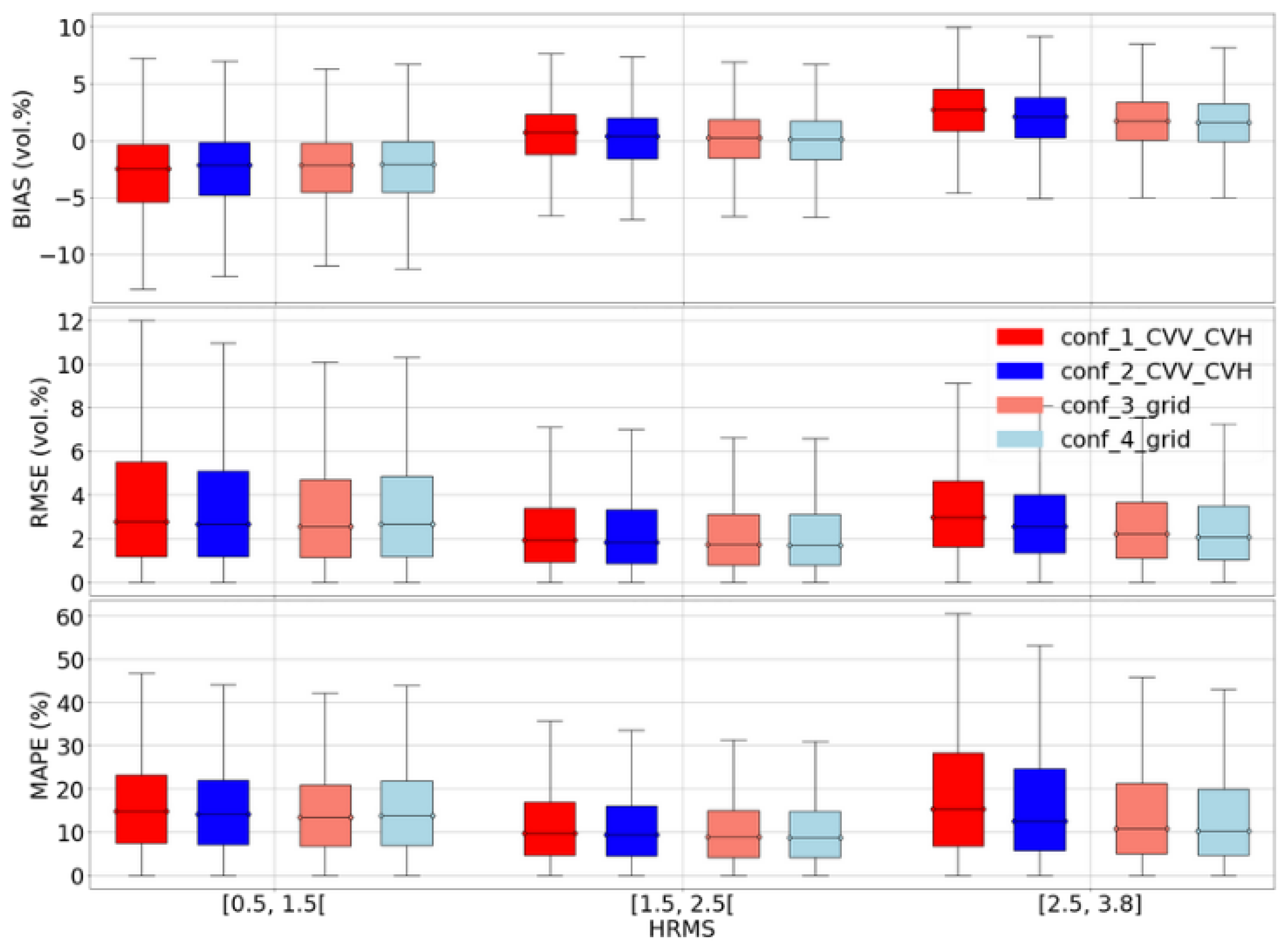
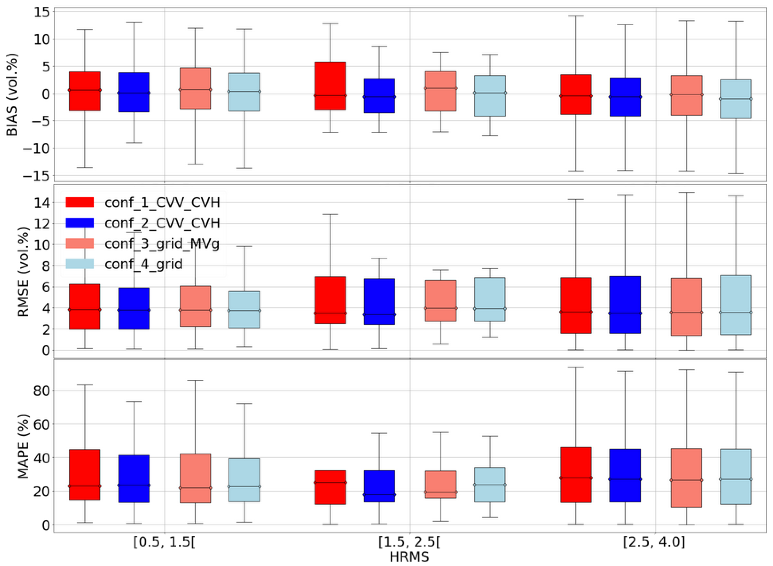
Combining VV and VH polarizations (configuration 1) consistently improves accuracy compared to using either polarizations individually. Separating the estimation domain into dry and wet conditions (configuration 2) highlights the importance of using a priori information on the global soil moisture state in the study site, yielding even better results when both VV and VH polarizations are used, with about 14% gain using the synthetic dataset and 5% gain on the real dataset in RMSE compared to the best configuration without domain separation. Incorporating grid information (configuration 3) optimizes accuracy without the need for weather information with about an 18% gain on the synthetic dataset (slightly better than the configuration that separates the estimation domain using weather information) and a 5% gain on the real dataset in RMSE compared to the first configuration. Finally, while integrating soil roughness estimates (configuration 4) does slightly enhance estimation accuracy, the improvements are negligible as to the complexity of the architecture (five NNs compared to just one). Overall, the combined use of VV and VH polarizations and incorporating grid information offers the best soil moisture estimation accuracy. This approach led to an RMSE on soil moisture of 3.5 vol.% on the synthetic dataset and 5.9 vol.% using the real dataset. These performances are similar to accuracies obtained with the top-performing configuration that leverages a priori weather information. The use of soil roughness estimates provides a marginal contribution to the inversion process.

Our Sentinel-1 signal inversion procedures have revealed limitations. Firstly, the accuracy of the inversion model based on the use of grid information or incorporating a priori information on soil moisture (dry to slightly wet condition or very wet condition) can be compromised due to the inappropriate choice of a dry or wet network for estimating soil moisture, especially in areas with irrigation practices. Secondly, the results from configuration 4, which estimates soil roughness, are inconclusive due to the instrumental characteristics of the Sentinel-1 sensor. Indeed, the C-band of Sentinel-1 is not the optimum wavelength for soil roughness mapping as well as the incidence angles which are lower than 40–45° for a wide part of Sentinel-1 images. Lastly, the high dependence of the radar signal on both soil roughness and moisture content leads to an ambiguity in the estimation of soil moisture when the inversion model estimates only the soil moisture without taking into account roughness or when the inversion model cannot estimate correctly both soil roughness and moisture content (SAR layers in the input are insufficient). Despite these limitations, integrating coarse soil moisture information (average moisture over large areas) has been demonstrated to improve soil moisture estimation at the plot scale.

The scope of this study was purposefully limited to bare soil to ensure a streamlined analysis by eliminating the effect of vegetation on the signal radar over agricultural plots. Having successfully conducted an analysis with bare soil, the methodology could be improved by utilizing the Water Cloud Model (WCM), which incorporates not only bare soil conditions but also vegetated soil. This model efficiently caters to scenarios involving both bare and vegetated soils. With this expansion, we could potentially apply our method broadly to estimate soil moisture on agricultural plots regardless of whether they are bare or vegetated. This constitutes a promising avenue for future research and applications.

References

1. Chaudhary, M.T.; Piracha, A. Natural Disasters-Origins, Impacts, Management. Encyclopedia 2021, 1, 1101–1131. [Google Scholar] [CrossRef]
2. Baghdadi, N.; Zribi, M. Characterization of Soil Surface Properties Using Radar Remote Sensing. Land Surf. Remote Sens. Cont. Hydrol. 2016, 1–39. [Google Scholar] [CrossRef]
3. Ulaby, F.T.; Moore, R.K.; Fung, A.K. Microwave Remote Sensing: Active and Passive. Volume I: Microwave Remote Sensing Fundamentals and Radiometry. In International Microwave Remote Sensing Fundamentals and Radiometry; Artech House: Norwood, MA, USA, 1981. [Google Scholar]
4. Dubois, P.C.; van Zyl, J.; Engman, T. Measuring Soil Moisture with Imaging Radars. Int. IEEE Trans. Geosci. Remote Sens. 1995, 33, 915–926. [Google Scholar] [CrossRef] [Green Version]
5. Holah, N.; Baghdadi, N.; Zribi, M.; Bru, A.; King, C. Potential of ASAR/ENVISAT for the characterization of soil surface parameters over bare agricultural fields. Remote Sens. Environ. 2005, 96, 78–86. [Google Scholar] [CrossRef] [Green Version]
6. Mattia, F.; Satalino, G.; Pauwels, V.R.N.; Loew, A. Soil moisture retrieval through a merging of multi-temporal L-band SAR data and hydrologic modeling. Hydrol. Earth Syst. Sci. 2009, 13, 343–356. [Google Scholar] [CrossRef] [Green Version]
7. Hamze, M.; Baghdadi, N.; El Hajj, M.; Zribi, M.; Bazzi, H.; Cheviron, B.; Faour, G. Integration of L-Band Derived Soil Roughness into a Bare Soil Moisture Retrieval Approach from C-Band SAR Data. Remote Sens. 2021, 13, 2102. [Google Scholar] [CrossRef]
8. Tang, Q.H.; Gao, H.; Lu, H.; Lettenmaier, D. Remote sensing: Hydrology. Prog. Phys. Geogr. 2009, 33, 490–509. [Google Scholar] [CrossRef]
9. Knipper, K.R.; Hogue, T.S.; Franz, K.J.; Scott, R.L. Downscaling SMAP and SMOS soil moisture with moderate-resolution imaging spectroradiometer visible and infrared products over southern Arizona. Int. J. Appl. Remote Sens. 2017, 11, 026021. [Google Scholar] [CrossRef] [Green Version]
10. Schwerdt, M.; Schmidt, K.; Tous Ramon, N.; Klenk, P.; Yague-Martinez, N.; Prats-Iraola, P.; Zink, M.; Geudtner, D. Independent System Calibration of Sentinel-1B. Remote Sens. 2017, 9, 511. [Google Scholar] [CrossRef] [Green Version]
11. Fung, A.K. Microwave Scattering and Emission Models and Their Applications; Artech House: Boston, MA, USA, 1994. [Google Scholar]
12. Zribi, M.; Taconet, O.; Le Hégarat-Mascle, S.; Vidal-Madjar, D.; Emblanch, C.; Loumagne, C.; Norm, M. Backscattering behavior and simulation comparison over bare soils using SIRC/XSAR and ERASME 1994 data over Orgeval. Remote Sens. Environ. 1997, 59, 256–266. [Google Scholar] [CrossRef]
13. Baghdadi, N.; King, C.; Chanzy, A.; Wingneron, J.-P. An empirical calibration of IEM model based on SAR data and measurements of soil moisture and surface roughness over bare soils. Int. J. Remote Sens. 2002, 23, 4325–4340. [Google Scholar] [CrossRef]
14. Baghdadi, N.; Gherboudj, I.; Zribi, M.; Sahebi, M.; Bonn, F.; King, C. Semi-empirical calibration of the IEM backscattering model using radar images and moisture and roughness field measurements. Int. J. Remote Sens. 2004, 25, 3593–3623. [Google Scholar] [CrossRef]
15. Chen, K.-S.; Wu, T.-D.; Tsang, L.; Li, Q.; Shi, J.; Fung, A.K. Emission of rough surfaces calculated by the integral equation method with comparison to three-dimensional moment method simulations. IEEE Trans. Geosci. Remote Sens. 2003, 41, 90–101. [Google Scholar] [CrossRef]
16. El Hajj, M.; Baghdadi, N.; Zribi, M.; Bazzi, H. Synergic use of Sentinel-1 and Sentinel-2 images for operational soil moisture mapping at high spatial resolution over agricultural areas. Remote Sens. 2017, 9, 1292. [Google Scholar] [CrossRef] [Green Version]
17. Nativel, S.; Ayari, E.; Rodriguez-Fern, N.; Baghdadi, N.; Madelon, R.; Albergel, C.; Zribi, M. Hybrid Methodology Using Sentinel-1/Sentinel-2 for Soil Moisture Estimation. Remote Sens. 2022, 14, 2434. [Google Scholar] [CrossRef]
18. Chung, J.; Lee, Y.; Kim, J.; Jung, C.; Kim, S. Soil Moisture Content Estimation Based on Sentinel-1 SAR Imagery Using an Artificial Neural Network and Hydrological Components. Remote Sens. 2022, 14, 465. [Google Scholar] [CrossRef]
19. Reza Mirsoleimani, H.; Sahebi, M.; Baghdadi, N.; El Hajj, M. Bare Soil Surface Moisture Retrieval from Sentinel-1 SAR Data Based on the Calibrated IEM and Dubois Models Using Neural Networks. Sensors 2019, 19, 3209. [Google Scholar] [CrossRef] [Green Version]
20. Bazzi, H.; Baghdadi, N.; El Hajj, M.; Zribi, M. Potential of Sentinel-1 Surface Soil Moisture Product for Detecting Heavy Rainfall in the South of France. Sensors 2019, 19, 802. [Google Scholar] [CrossRef] [PubMed] [Green Version]
21. Bazzi, H.; Baghdadi, N.; Ienco, D.; El Hajj, M.; Zribi, M.; Belhouchette, H.; Escorihuela, M.J.; Demarez, V. Mapping Irrigated Areas Using Sentinel-1 Time Series in Catalonia, Spain. Remote Sens. 2019, 11, 1836. [Google Scholar] [CrossRef] [Green Version]
22. Choker, M.; Baghdadi, N.; Zribi, M.; El Hajj, M.; Paloscia, S.; Verhoest, N.; Lievens, H.; Mattia, F. Evaluation of the Oh 1836,Dubois and IEM models using large dataset of SAR signal and experimental soil measurements. Water 2017, 9, 38. [Google Scholar] [CrossRef] [Green Version]
23. Baghdadi, N.; Saba, E.; Aubert, M.; Zribi, M.; Baup, F. Comparison between backscattered TerraSAR signals and simulations from the radar backscattering models IEM, Oh, and Dubois. IEEE Geosci. Remote Sens. Lett. 2011, 8, 1160–1164. [Google Scholar] [CrossRef]
24. Baghdadi, N.; Zribi, M. Evaluation of Radar Backscatter Models IEM, OH and Dubois Using Experimental Observations. Int. J. Remote Sens. 2006, 27, 3831–3852. [Google Scholar] [CrossRef]
25. Walker, J.P.; Willgoose, G.R.; Kalma, J.D. In situ measurement of soil moisture: A comparison of techniques. J. Hydrol. 2004, 293, 85–99. [Google Scholar] [CrossRef]
26. Levenberg, K. A Method for the Solution of Certain Non-linear Problems in Least Squares. Q. Appl. Math. 1994, 2, 164–168. [Google Scholar] [CrossRef] [Green Version]
27. Baghdadi, N.; Zribi, M.; Loumagne, C.; Ansart, P.; Anguela, T.P. Analysis of TerraSAR-X data and their sensitivity to soil surface parameters over bare agricultural fields. Remote Sens. Environ. 2008, 112, 4370–4379. [Google Scholar] [CrossRef] [Green Version]
28. Baghdadi, N.; King, C.; Bourguignon, A.; Remond, A. Potential of ERS and RADARSAT data for surface roughness monitoring over bare agricultural fields: Application to catchments in Northern France. Int. J. Remote Sens. 2002, 23, 3427–3442. [Google Scholar] [CrossRef]
29. Baghdadi, N.; Gaultier, S.; King, C. Retrieving surface roughness and soil moisture from SAR data using neural network. Can. J. Remote Sens. 2002, 28, 701–711. [Google Scholar] [CrossRef]
30. Bazzi, H.; Baghdadi, N.; Fayad, I.; Zribi, M.; Belhouchette, H.; Demarez, V. Near Real-Time Irrigation Detection at Plot Scale Using Sentinel-1 Data. Remote Sens. 2020, 12, 1456. [Google Scholar] [CrossRef]
Figure 1. Locator map of the Montpellier study area in the Occitanie region of France. In green are the bare reference fields on which soil moisture and roughness measurements were collected.
Remotesensing 15 03502 g001
Figure 2. Locator map of the Kairouan study area in the Kairouan Governorate of Tunisia. In green are the bare reference fields on which soil moisture measurements are collected.
Remotesensing 15 03502 g002
Figure 3. Accuracy metrics (bias, RMSE and MAPE) on soil moisture estimates of the 4 configurations using the synthetic validation set.
Remotesensing 15 03502 g003
Figure 4. N sensitivities on soil moisture ranges for the synthetic validation set. Only the best subcase of each configuration is plotted, conf_3_grid and conf_4_grid were plotted without a priori information on MVp.
Remotesensing 15 03502 g004
Figure 5. N sensitivities on soil roughness (HRMS) for the synthetic validation set. Only the best subcase of each configuration is plotted, conf_3_grid and conf_4_grid were plotted without a priori information on MVp.
Remotesensing 15 03502 g005
Figure 6. Accuracy metrics (Bias, RMSE and MAPE) on soil moisture estimates of the 4 configurations using the real dataset.
Remotesensing 15 03502 g006
Figure 7. Model sensitivity on soil moisture for the real dataset. Only the best subcase of each configuration is plotted, case_3_grid_MVg and conf_4_grid were plotted without a priori information on MVp.
Remotesensing 15 03502 g007
Figure 8. Model sensitivity across different soil roughness ranges for the real dataset. Only the best subcase of each configuration is plotted; case_3_grid_MVg and conf_4_grid were plotted without a priori information on MVp.
Remotesensing 15 03502 g008
Figure 9. Difference between estimated and measured soil moisture on recently irrigated plots (green points) and non-irrigated plots (red points) in Kairouan site. The Config_3_grid_MVg neural networks were used to estimate the soil moisture.
Remotesensing 15 03502 g009
Figure 10. Model sensitivity on soil moisture for the Montpellier dataset. Only the best subcase of each configuration is plotted, case_3_grid_MVg and conf_4_grid were plotted without a priori information on MVp.
Remotesensing 15 03502 g010
Figure 11. Model sensitivity on soil moisture for the Kairouan dataset. Only the best subcase of each configuration is plotted, case_3_grid and conf_4_grid were plotted without a priori information on MVp.
Remotesensing 15 03502 g011