Article

The Correction Method of Water and Fresnel Reflection Coefficient for Soil Moisture Retrieved by CYGNSS

1
Chengdu Institute of Surveying and Investigation, Chengdu 610081, China
2
Urban Informatization Surveying and Mapping Engineering Technology Research Center of Sichuan, Chengdu 610081, China
3
The Third Geographical Information Mapping Institute of Natural Resources Ministry, Chengdu 610100, China
4
School of Geodesy and Geomatics, Wuhan University, Wuhan 430079, China
5
Hubei Luojia Laboratory, Wuhan 430079, China
*
Author to whom correspondence should be addressed.
Remote Sens. 2023, 15(12), 3000; https://doi.org/10.3390/rs15123000
Submission received: 8 April 2023 / Revised: 20 May 2023 / Accepted: 6 June 2023 / Published: 8 June 2023
(This article belongs to the Special Issue GNSS-R Earth Remote Sensing from SmallSats)

Abstract

:
Spaceborne GNSS-R technology is a new remote sensing method for soil moisture monitoring. Focusing on the significant influence of water on the surface reflectivity of CYGNSS, this paper improved the removal method of water influence according to the spatial resolution of CYGNSS data. Due to the disturbance effect of the incident angle, microwave frequency and soil type on the Fresnel reflection coefficient in surface reflectivity, a normalization method of Fresnel reflection coefficient was proposed after analyzing the data characteristics of variables in the Fresnel reflection coefficient. Finally, combined with the soil moisture retrieval method of linear equation, the accuracy was compared and verified by using measured data, SMAP products and official CYGNSS products. The results indicate that the normalization method of the Fresnel reflection coefficient could effectively reduce the influence of relevant parameters on the Fresnel reflection coefficient, but the normalization effect became worse at large incident angles (greater than 65°). Compared with the official CYGNSS product, the retrieval accuracy of optimized soil moisture was improved by 10%. The method proposed in this paper will play an important reference role in the study of soil moisture retrieval using spaceborne GNSS-R data.

Graphical Abstract

1. Introduction

Soil moisture is of great value in understanding plant physiological activities, hydrometeorological processes, global energy exchange and agricultural production [1,2,3]. The distribution information of accurate soil moisture is not only of great significance for scientific research, but can also serve a number of practical applications. Spaceborne GNSS Reflectometry (GNSS-R) is an emerging remote sensing technology for reflecting soil moisture over a large area due to its advantages of a wide signal source, large data volume, short revisit time, low cost and low power consumption, etc. Its frequency band and high spatial-temporal resolution can effectively compensate for the shortcomings of optical remote sensing, which is easily obscured by clouds, and the low spatial resolution of microwave remote sensing products [4,5,6,7,8,9,10].
Since the UK TechDemoSat-1 (TDS-1) and Cyclone Global Navigation Satellite System (CYGNSS) satellites provide spaceborne GNSS-R data for free, the retrieval of soil moisture for spaceborne GNSS-R has gradually become a research hotspot. In order to effectively characterize the relationship between the surface reflectivity of CYGNSS and soil moisture, and thus obtain high accuracy retrieval results for soil moisture, a large number of modeling algorithms have been applied, such as linear models [11,12,13,14], machine learning [15,16,17] and deep learning [18], etc.
The reflection signal carrying water body information will weaken the sensitivity of the surface reflectivity of CYGNSS to soil moisture, and thus reduce the accuracy of soil moisture retrieval. Related studies have shown that a 25 m wide body of water can significantly affect the surface reflectivity of CYGNSS [11]. Therefore, Chew et al. [19], Wan et al. [20] and Zhu et al. [21] performed the removal of the water body effect on CYGNSS observations by means of external data sources such as the Global Surface Water Explorer (GSWE) and the water data of SMAP. The Fresnel reflection coefficient is one of the major component variables of CYGNSS surface reflectivity, and is directly related to the angle of incidence and the soil dielectric constant. The influence of the correlation parameters in the Fresnel reflection coefficient on CYGNSS surface reflectivity can be effectively weakened, which can improve the accuracy of soil moisture retrieval [22]. Al-Khaldi et al. [23] proposed the normalization method of the incident angle to correct the surface reflectivity of CYGNSS, and the results proved that the method could attenuate the effect of the incident angle in the Fresnel reflection coefficient. In addition, this method was also applied to the soil moisture product algorithm of CYGNSS developed by Chew et al. [11,23].
As the sampling frequency of CYGNSS increases, its spatial resolution changes and thus the original method for removing the influence of water bodies will mistakenly pick data carrying valid information. The Fresnel reflection coefficient is composed of the incident angle and the soil dielectric constant, which is directly related to the microwave frequency, soil temperature, soil type composition and soil moisture [24]. Current research has focused on attenuating the effects of incident angle and soil moisture on the Fresnel reflection coefficient, further resulting in a lack of complete analysis of the relevant influences in the Fresnel reflection coefficient and the establishment of a unified model to attenuate the effects of these parameters. Therefore, this paper first improved the removal method of observations affected by water bodies based on the analysis of CYGNSS data. Then, the variable response of the Fresnel reflection coefficient was analyzed in detail and the normalization method was proposed. Finally, the accuracy of soil moisture retrieval using CYGNSS was improved by combining the method of soil moisture retrieval with a linear model. After the introduction, Section 2 describes an overview of the study area and the adopted dataset. Section 3 presents proposed methods and the retrieval method of soil moisture. The results of the proposed method and soil moisture retrieval are displayed and appraised in Section 5. The discussion for results of the study is given in Section 5. Finally, the main conclusions for this study are given in Section 6.

2. Study Area and Data Source

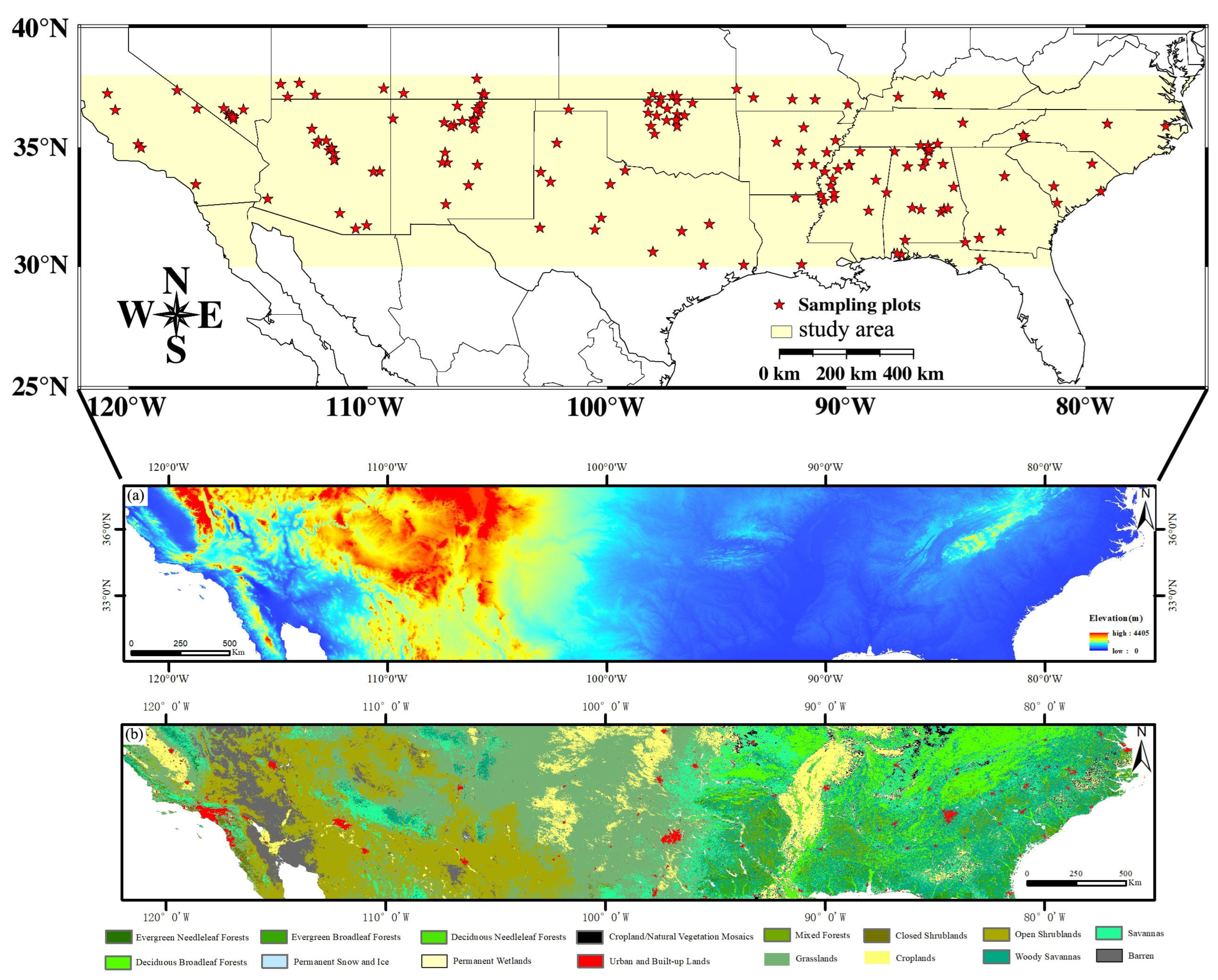
2.1. Study Area and Ground Measurements

The study area was located in the southern United States, covering 26 states with a geographical range of 75°~122°W and 30°~38°N (Figure 1). The region covers a vast area, with subtropical, temperate continental and tropical climates in the southeast, central and southwest. The southeast is warm and humid, the middle is cold in winter and hot in summer and the southwest has a large annual temperature difference of up to 25 °C. The topography of the entire region is high in the west and low in the east, and there is a clear topographic divide (100°W) in the middle of the region. The western part of this topographic divide is dominated by plateaus and mountains, while the eastern part is plains (Figure 1a). Based on the LC_Type1 (Scheme of global vegetation classification for IGBP) band of the MCD12Q1 product of MODIS, a map of vegetation cover types in the study area was obtained, as shown in Figure 1b.
The measured soil moisture data used in the study area were freely available to the public in terms of volumetric water content (m3/m3) and were derived from the International Soil Moisture Observation Network (ISMN; http://ismn.geo.tuwien.ac.at/networks, accessed on 6 November 2021). In this study, four monitoring networks, ARM, SCAN, SNOTEL and USCRN in ISMN, with a total of 160 measured monitoring points, were used from July 2019 to December 2021, with a soil moisture depth of 5 cm. Among these measurement stations of soil moisture, meaningless stations with values less than 0 cm3/cm3 or greater than 1 cm3/cm3 were excluded.

2.2. CYGNSS Data

CYGNSS is a constellation of eight satellites, each of which has four channels; i.e., thirty-two observations per second can be received. Due to the increase in CYGNSS sampling frequency after July 2019 (i.e., with 500 ms non-coherent accumulation), the resolution of CYGNSS is 3.5 × 0.5 km at this time. The CYGNSS data used in this study are the L1-level data of version 3.0 from July 2019 to December 2021, which can be downloaded from the official CYGNSS website (https://cygnss.engin.umich.edu/data-products/ (accessed on 6 November 2021)). To improve the quality of CYGNSS data, standard quality control and empirical quality control were performed [19]. The higher launch power of the GPS Block IIF satellite introduces uncertainty at peak power [25]. Removing these data will reduce the overall data volume by 30%. Therefore, this part of the data was chosen to be retained in this study. The power received by CYGNSS consists of both incoherent and coherent scattering components [26]. Most studies have been based on the assumption that the incoherent component is ignored and only the coherent scattering component is retained [11,12,14,20]. Therefore, based on the land scattering model of GNSS-R, the surface reflectivity Γ(θ) of CYGNSS can be readily derived, following the assumption that the coherent component dominates:
Γ ( θ ) = P r ( R t + R r ) 2 ( 4 π ) 2 P t G t G r λ 2
where Pr and Pt are, respectively, the reflected power received by the receiver and the transmitted power. λ is the carrier signal wavelength. Rr and Rt are, respectively, the distances from the receiver and transmitter to the specular reflection point. Gt and Gr are the transmitting antenna gain and receiving antenna gain, respectively.

2.3. SMAP Data

Soil Moisture Active and Passive (SMAP) is an Earth observation mission carrying an L-band radiometer and radar, which provides soil moisture and freeze–thaw data with a time-resolution of 2–3 days from NASA (https://nsidc.org/data/smap/smap-data.html (accessed on 6 November 2021)). In this study, soil moisture data (L3_SM_P) of SMAP L3 were used, which were obtained by retrieval using the Single Channel Algorithm (SCA) with a spatial resolution of 36 km. The time period was selected from July 2019 to December 2021. SMAP was divided into two types of data: daily 6:00 a.m. (descending orbit) and 18:00 p.m. (ascending orbit). It has been shown that the surface temperature homogenization at 6:00 a.m. is better than that at 18:00 p.m., and the retrieval accuracy is higher than that at 18:00 [27]. In this study, both descending orbit and ascending orbit data were incorporated and averaged to obtain soil moisture data of SMAP.

2.4. Water Body Data
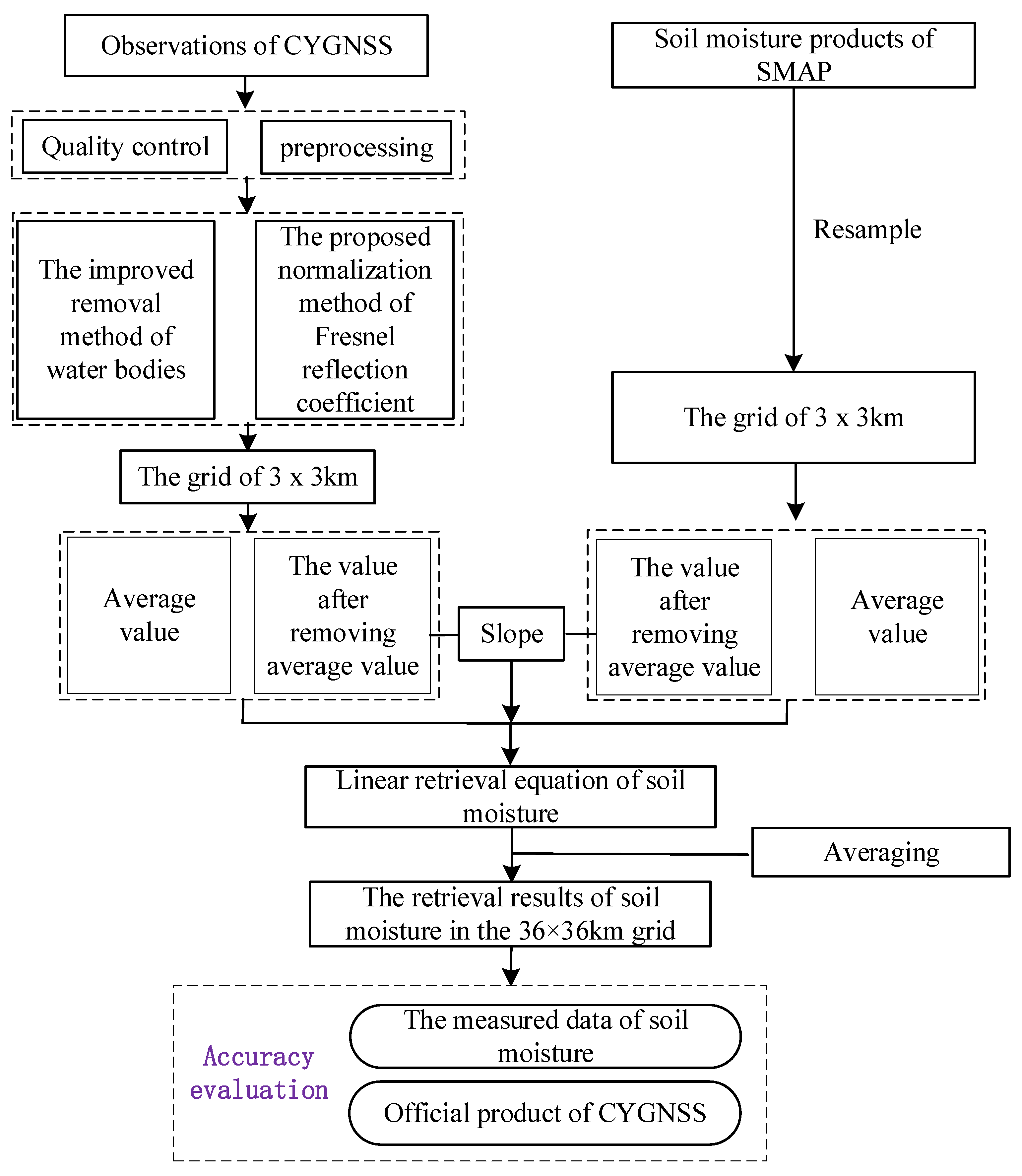
The water body data of GSWE came from a 30 m dataset produced based on optical images from Landsat satellites [28], with global coverage. GSWE released several sub-datasets, including Occurrence, Change, Seasonality, Recurrence, etc. Each sub-dataset consisted of a 10° × 10° grid with a total range of 60°S~80°N and 180°W~180°E. The “Seasonality” product was selected for this study, and the individual pixel values were classified on a scale of 1 to 12, indicating how many months of the year were inundated with water. In this case, all values greater than 1 were labeled as water bodies to facilitate the exclusion of observations influenced by water bodies. Since this study was in the southern region of the United States, a total of 12 Seasonality data were selected for the range of 30°N to 50°N and 130°W to 70°W. A Seasonality product from these data was shown in Figure 2. Due to the special and static nature for the time-resolution of Landsat data, the produced GSWE dataset could not be synchronized with the observation time of CYGNSS. However, this dataset could remove the observations affected by water bodies to some extent.

3. Methodology

In this study, the procedure for the retrieval of soil moisture using CYGNSS based on proposed methods was illustrated in Figure 3. The first step involved the quality control and processing of data used, such as CYGNSS, SMAP and GSWE. The surface reflectivity derived from CYGNSS was corrected using an improved method of water removal and the normalization method of the Fresnel reflection coefficient. A linear regression equation of soil moisture was established by combining the resampled soil moisture product of SMAP with the corrected surface reflectivity. Finally, the results of soil moisture were obtained by averaging the retrieved soil moisture, and the accuracy was comparatively verified based on the measured data, SMAP products and CYGNSS products.

3.1. Removal of Water

The current solution for observations influenced by water bodies is to exclude observations that carry information about water bodies [19,20]. A square grid of 7 × 7 km to exclude observations influenced by water bodies was designed by Chew et al. [19], based on the “Seasonality” product from GSWE data. According to the research of Chew et al. [19], an improved method for removing observations affected by water bodies in a 3 × 3 km square grid was proposed by analyzing the characteristics of CYGNSS data. The process was as follows:
Step 1: Based on the latitude and longitude of the specular reflection point from CYGNSS, its corresponding location in the “Seasonality” product was searched.
Step 2: A square grid of 3 × 3 km was created, with this corresponding location as the center.
Step 3: When there was a value marked as 1 (i.e., there is a water body) in this 3 × 3 km square grid, then the point was eliminated, i.e., the specular reflection point was eliminated.
Step 4: The above process was repeated to complete the removal of specular reflection points affected by water bodies.
The removal diagram of the observations affected by the water was shown in Figure 4:

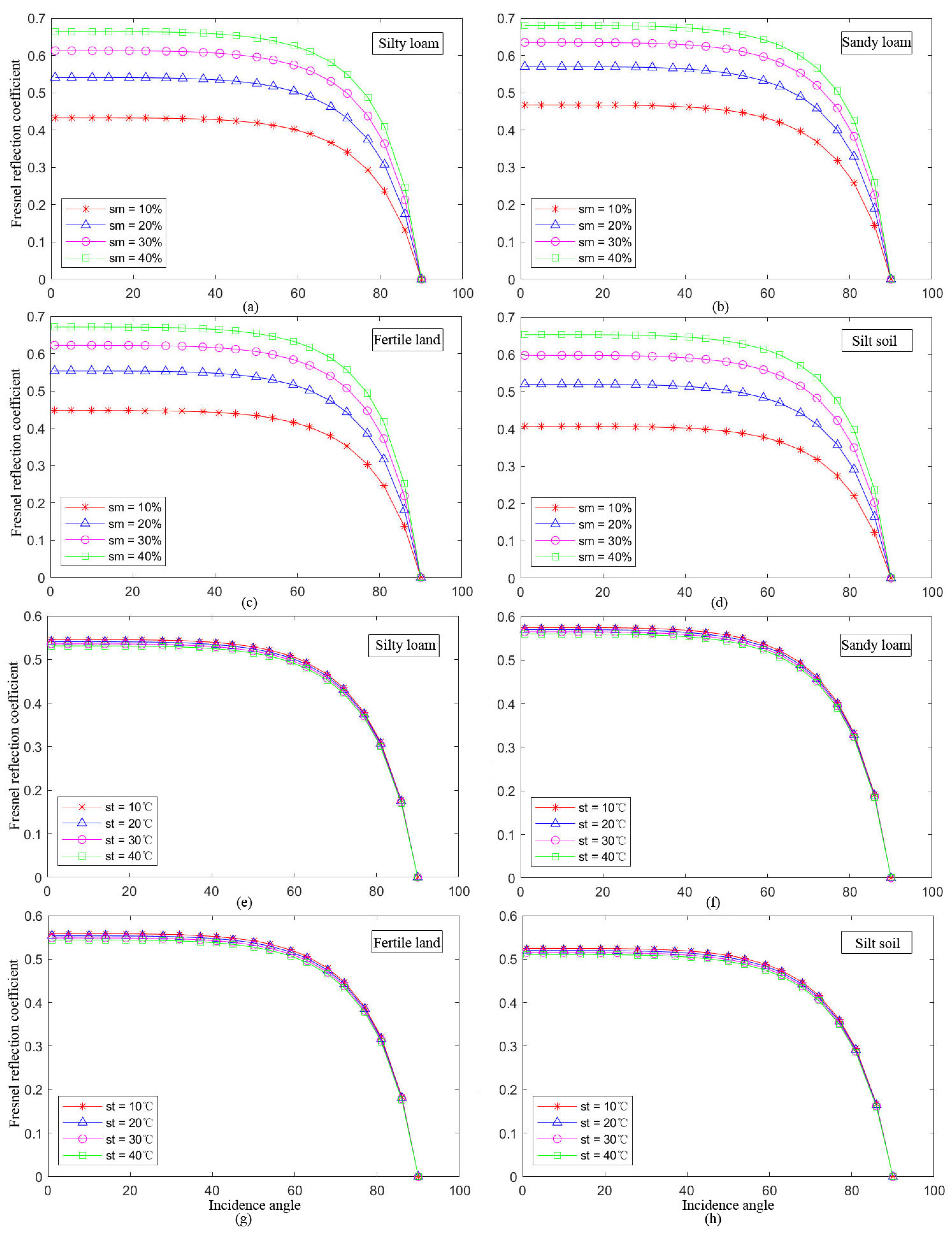
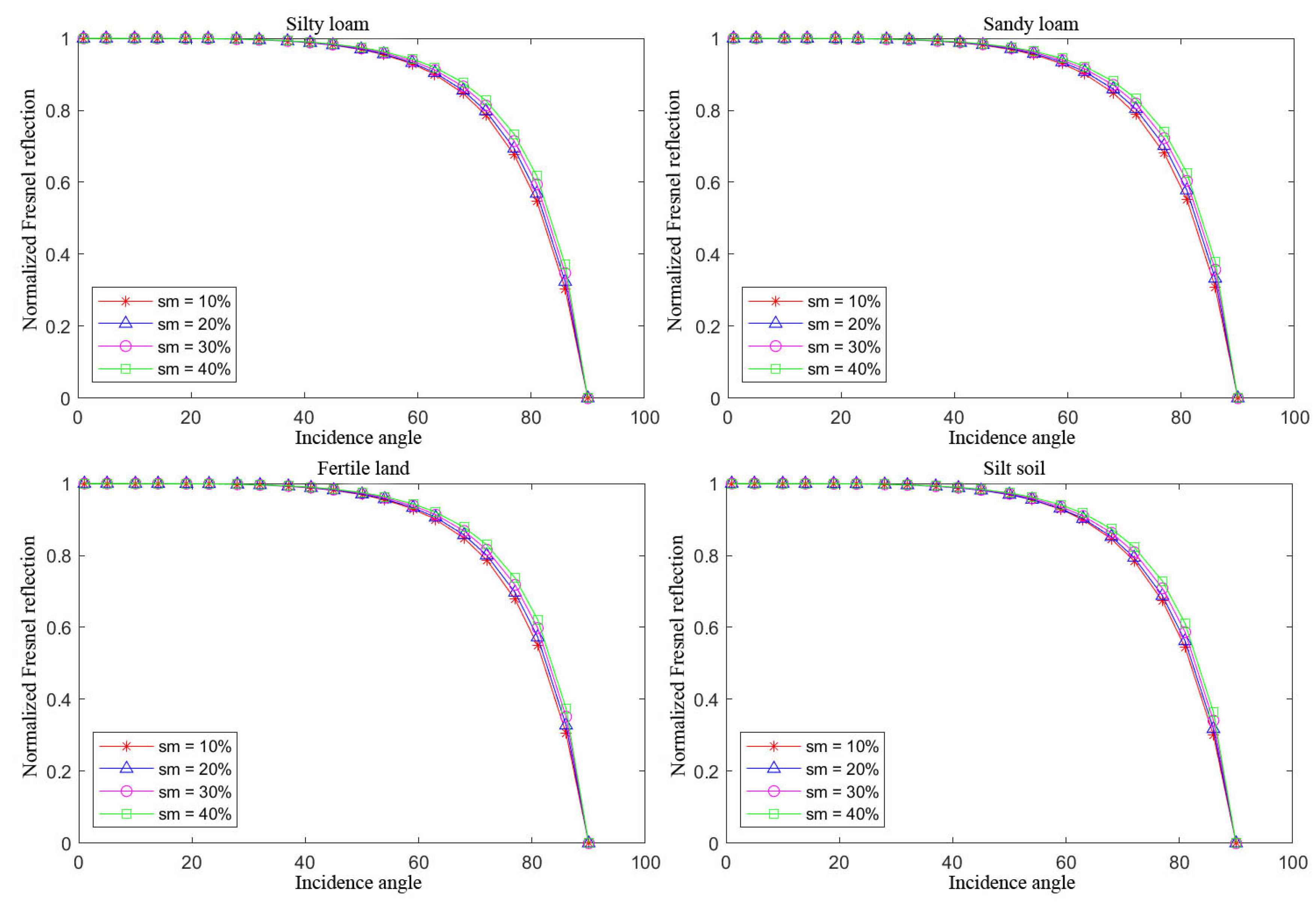
3.2. The Normalization of the Fresnel Reflection Coefficient

According to the Kirchhoff approximation, the surface reflectivity Γ(θ) of CYGNSS can be further expressed as [29,30,31]:
Γ ( θ ) = R l r ( θ ) 2 γ exp ( ( 2 k σ cos θ ) 2 )
γ is the vegetation attenuation term; exp ( ( 2 k σ cos θ ) 2 ) is the attenuation term of surface roughness; and Rlr(θ) is the Fresnel reflection coefficient, which is a function of the incident angle θ and the soil dielectric constant ε [32]. ε is calculated by the Dobson model [24], which is adapted to the frequency range of 0.3–1.3 Ghz and 1.4–18 Ghz and consists of microwave frequency, soil temperature, soil type composition and soil moisture:
ε s o i l α = 1 + p b p s ε s α 1 + m v β ε f w α m v 1 α
β = 1.2748 0.00519 P s a n d 0.00152 P c l a y
where Pb and Ps are the bulk density of soil and the density of the solid medium in soil, respectively. α is generally 0.65, and εfw and εs are the permittivity of free water and solid soil, respectively. mv is soil moisture. Psand and Pclay represent the sand and clay contents of soil (%), respectively.
According to Formulas (3) and (4), the response of these relevant variables to the Fresnel reflection coefficient was shown in Figure 5. Soil type parameters refer to the table of physical parameters published by the Dobson model [24] (Table 1).
From Figure 5a–d, it can be seen that the Fresnel reflection coefficients obtained from different soil moisture values varied greatly under the condition of constant soil temperature and the same soil type. For a constant soil temperature and the same soil moisture, the Fresnel reflection coefficient corresponding to different soil types was also different. The above results indicate that differences in the soil type and soil moisture can lead to changes in the Fresnel reflection coefficient. Figure 5e–h show the response of the Fresnel reflection coefficient for a constant value of soil moisture and different soil temperatures. It can be observed that the changes in Fresnel reflection coefficients obtained from soil temperature differences were small relative to those caused by changes in soil moisture. Of course, differences in the Fresnel reflection coefficient between soil types are always present. Moreover, in Figure 5, the Fresnel reflection coefficient becomes smaller and smaller, with an increasing incident angle regardless of the differences in soil moisture, temperature and soil type, indicating that the incident angle plays a very important role.
In this study, a normalization method of the Fresnel reflection coefficient was proposed to reduce the influence of relevant parameters on the Fresnel reflection coefficient, and thus reduced the surface reflectivity error of CYGNSS caused by the Fresnel reflection coefficient and improved the accuracy of soil moisture retrieval. The process of establishing this method consisted of four steps in total.
Step 1: A database of Fresnel reflection coefficients with incident angle as the independent variable was created by freely combining values in the range of soil moisture, soil temperature, soil type and incident angle. Soil moisture, soil temperature and incident angle were limited to [1, 100], [1, 60] and [1, 90], respectively. The increments for these three parameters were set as 1%, 1 °C and 1°, respectively. Soil types referred to the physical parameters of the Dobson model (Table 1). Microwave frequency was set to 1.57542 GHz. Through the combination of the above variables, a total of 2,160,000 Fresnel reflection coefficient values in the range of incident angles from 1 to 90° were formed.
Step 2: Based on the combination of variables in Step 1, a database of a total of the values of 2,160,000 Fresnel reflection coefficients with an incident angle of 0° was additionally composed.
Step 3: Based on the database created in Step 1 and Step 2, the correction variable was obtained using the following equation:
R l r ( θ ) c o r = R l r ( θ ) / R l r ( 0 )
where Rlr(θ)cor is the corrected Fresnel reflection coefficient, Rlr(θ) is the Fresnel reflection coefficient obtained from Step 1 and Rlr(0) is the Fresnel reflection coefficient for an incident angle of 0° in Step 2.
Step 4: With incident angle as the independent variable and corrected Fresnel reflection coefficient values of 2,160,000 as the dependent variable, the functional relationship between corrected Fresnel reflection coefficient and incident angle (1–90°) was established. A functional expression for the angle of incidence was as follows:
f ( θ ) = a · exp ( b · θ ) + c
where a, b and c are all empirical parameters, which can be obtained by solving the parameters using the least square method.

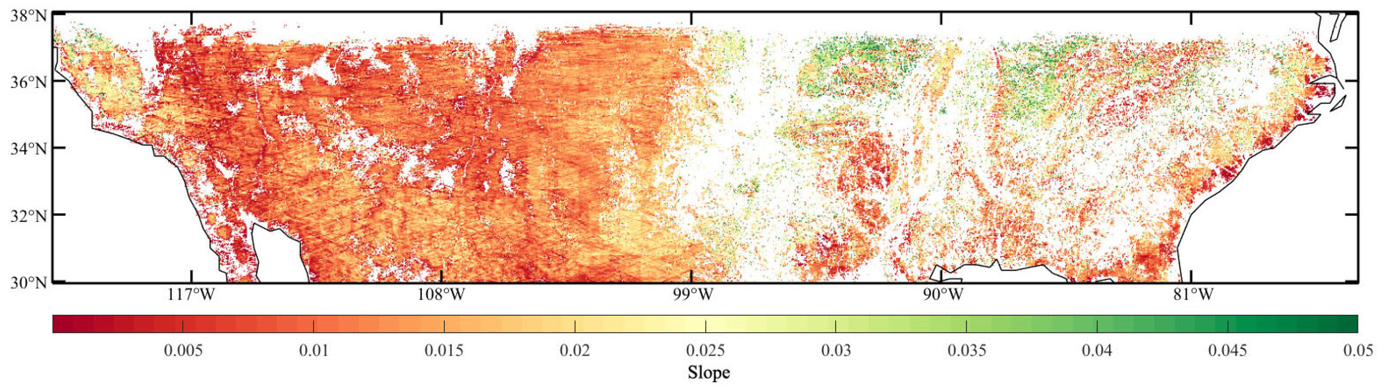
3.3. The Retrieval Algorithm of Soil Moisture

In this study, the soil moisture retrieval algorithm of the linear regression equation proposed by Chew et al. [11] was based on the assumption that the surface reflectivity obtained from CYGNSS data is linearly correlated with the soil moisture of SMAP, and this linear correlation presents spatial variation and does not vary with time. The spatial resolution of CYGNSS is much smaller than the SMAP product, and the surface reflectivity varies depending on land cover and topography. Therefore, to effectively attenuate the effects of vegetation cover and topography, surface reflectivity corrected by the proposed method and soil moisture products of SMAP were sampled on a 3 × 3 km grid using the nearest neighbor sampling method [33,34,35], and thus soil moisture was retrieved. Among them, the nearest neighbor sampling method did not change the original pixel values of the SMAP products during resampling. The SMAP products of the 36 × 36 km grid were sampled into the 3 × 3 km grid, i.e., all 3 × 3 km grids within a 36 × 36 km grid have the same values. The expression was as follows:
S M C Y G N S S , t = β · ( Γ t Γ c a l ¯ ) + S M S M A P , c a l ¯
SMCYGNSS,t is the soil moisture retrieved with CYGNSS, Γ t is the corrected surface reflectivity of CYGNSS and Γ c a l ¯ and S M S M A P , c a l ¯ are the mean values of corrected surface reflectivity from CYGNSS and soil moisture products of SMAP during the modeling time, respectively. β is the slope, representing the slope of the SMAP products and corrected surface reflectivity after removing S M S M A P , c a l ¯ and Γ c a l ¯ at the modeling time. If there were less than three sampling points of CYGNSS in a 3 × 3 km grid, the β of the grid was not calculated. The value of β will be used to estimate the soil moisture during the validation period. Soil moisture retrieval was performed for the 3 × 3 km grid according to the above process, and then the soil moisture result of 3 × 3 km were aggregated and averaged to the 36 × 36 km grid. The mean values for soil moisture of all 3 × 3 km within the 36 × 36 km grid were used as the retrieval values of soil moisture of the final 36 × 36 km grid.

4. Results

4.1. The Correction Results of the Fresnel Reflection Coefficient

Figure 6 shows the responses of four soil types at the same soil temperature and different soil moisture after the normalization method of Fresnel reflection coefficient. It can be seen that the effect of differences in the soil moisture and soil type on the Fresnel reflectance coefficient was significantly weakened compared to the previous one, indicating that the surface reflectivity of CYGNSS corrected by the proposed method can significantly attenuate the effect of factors related to the Fresnel term. However, when the incident angle was larger (greater than 65°), the normalization effect became less effective. Excessive incident angles can significantly affect the quality of CYGNSS data [11,23], and this method used should keep the incident angle less than 65°.

4.2. Estimation of Soil Moisture

Based on the study area and data, data from July 2019 to December 2020 (modeling time) were used for modeling, and data from 2021 (validation time) were used to retrieve the soil moisture (Figure 7). Accuracy was evaluated in terms of unbiased root-mean-square error (ubRMSE) and Pearson correlation coefficient (R) based on soil moisture data from measured sites. Figure 7 provides the retrieval maps of soil moisture for any time in the four seasons: spring, summer, fall and winter. It can be seen that the western region showed a significantly lower soil moisture phenomenon in four seasons in 2021, while the eastern part was relatively much wetter. Based on the occurrence of the phenomenon of annual drought in the western United States in 2021 (US Drought Monitor, USDM), the retrieval results of soil moisture in this study were more consistent with the actual situation.
The sites where the retrieved soil moisture was in good agreement with the measured data are shown in Figure 8. It can be seen that the retrieval results of soil moisture at these four stations were dense, and all of them could capture the changes in measured soil moisture and reflect the changes in low and high values of soil moisture.

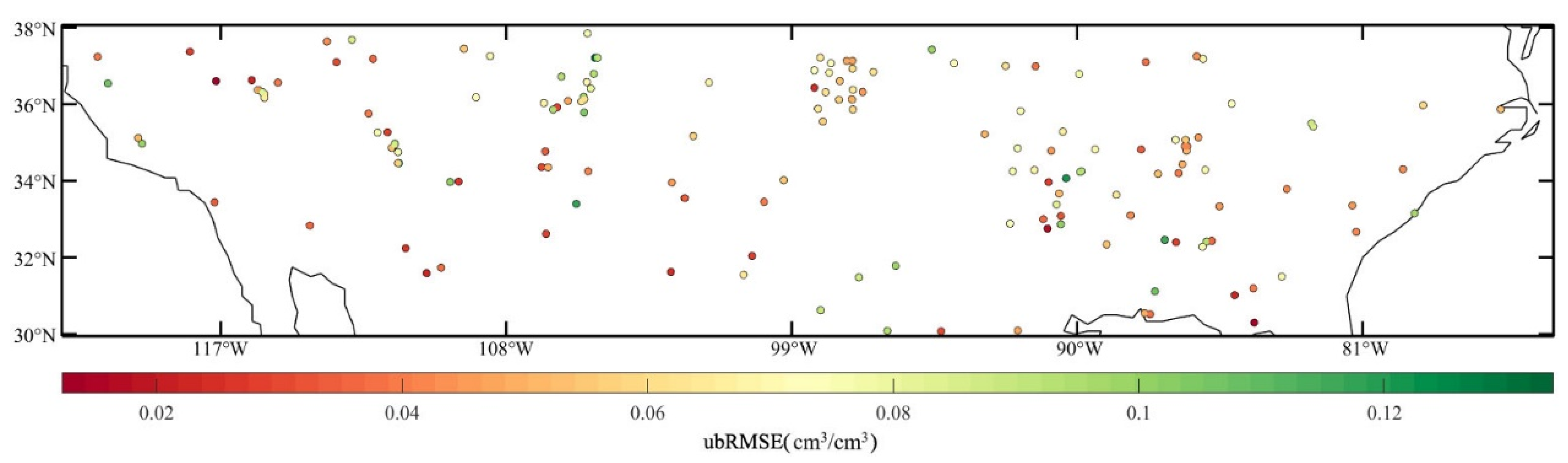
4.3. Validation of Soil Moisture

The data from the measured sites were based on the results of point measurements, and the soil moisture results were obtained in this study for a 36 × 36 km grid. It is reasonable to use the average value of measured soil moisture in a large area grid as the true value, but there is a lack of such a design for a soil moisture station. Therefore, related studies have used the values of a single measured site to verify the accuracy of soil moisture retrieval [11,14,20]. The accuracy validation of soil moisture results using the retrieval method of this study was executed based on the data measured in the study area. Table 2 and Table 3 provide statistics on the accuracy comparison between the SMAP and the soil moisture retrieval results using the method of this study, based on the data of each measured site within the experimental area.
The average ubRMSE for the retrieval results of soil moisture in this study was 0.061 cm3/cm3 at 160 measured stations, with an average correlation of 0.4. However, SMAP products presented a better retrieval performance for the soil moisture (ubRMSE = 0.056 cm3/cm3, R = 0.55). In ubRMSE, the median and mean values of soil moisture retrieved by the method used in this study in the four monitoring networks were worse than those of SMAP, with relatively large standard deviations. The same was true in the correlation. Areas with low or no variation in soil moisture during the validation time resulted in a lower correlation, possibly because the effect of random noise was amplified. The soil moisture values retrieved by CYGNSS may have had more noise than those of SMAP due to the lack of complete coverage of the soil moisture time series in part of the grid.
In order to show the effectiveness of the method in this study, the accuracy indexes for the CYGNSS product (i.e., UCAR/CU) and the results of this study at the common measured sites were systematically counted [19] (Table 4 and Table 5). Since the UCAR/CU product was only updated until August 2020, a comparison of the accuracy metric results from this study and the accuracy metric results from the paper by Chew et al. [19] was performed.
Compared with the UCAR/CU product, the accuracy of the soil moisture results obtained by this study was significantly improved, with the average ubRMSE of SCAN, SNOTEL and USCRN improved by 3.5%, 19% and 10%, respectively. The average ubRMSE at 88 measured sites was improved by 10%. The standard deviation and median had smaller values relative to those of UCAR/CU, indicating that the accuracy of this study remained more stable. In terms of correlation, the results of this study were the same as those of UCAR/CU. Furthermore, the median of the results of two measured networks (SNOTEL and USCRN) was relatively high, and the overall standard deviation was larger.

5. Discussion

From Figure 7, there were more blank points in the retrieval map of soil moisture in this study, which may be due to the lack of values in the 3 × 3 km grid, resulting in blank values when 3 × 3 km was aggregated to 36 × 36 km. Therefore, the number of surface reflectivity points of CYGNSS contained in each grid at the 3 km spatial resolution in the modeling time was counted (Figure 9). The number of grids with surface reflectivity points fewer than 20, between 20 and 40, between 40 and 80, and greater than 80 accounted for 40%, 19.7%, 29.3% and 11% of the total number of grids, respectively. As shown in Figure 9, a large number of null values appeared in the central and eastern parts of the study area; the western part presented more grids with fewer surface reflectivity points; grids with fewer than 20 grid points accounted for 40% of the total number of grids in the study area during the modeling time. The absence of values for surface reflectivity points of CYGNSS made the retrieved soil moisture results show the phenomenon of a blank value, probably because some of the surface reflectivity points of CYGNSS were removed by the method of a water body, especially in the central and eastern regions, as well as in the seaward regions, where a large number of water bodies exist. However, after analyzing the results without using the removal method of water bodies, it was found that this method was not the main reason for the appearance of few reflection points and null places, but rather the non-coherent accumulation times of CYGNSS receivers and the irregular distribution of specular reflection points resulted in the sparse spatial distribution of surface reflectivity points of CYGNSS at 3 km spatial resolution and the low distribution of observation points.
The slope was calculated based on the SMAP product and the corresponding surface reflectivity of CYGNSS after removing the average value. A temporal resolution of 2~3 days for SMAP and the property of random distribution of CYGNSS would reduce the number of mutually matched values. Meanwhile, if there were fewer than three matching values in the modeling time, the corresponding slope was not calculated. However, the number of grids with fewer than three in this part was 1% of the total number of grids. Therefore, the slope of the linear equation is another reason for the existence of blank values in the retrieval results of soil moisture (Figure 10).
The soil moisture results obtained in this study varied across the measured soil moisture networks (Table 2 and Table 3), and these were projected onto maps for further analysis, as shown in Figure 11 and Figure 12. The ubRMSE for most of the measured sites were below the mean value of 0.061 cm3/cm3, accounting for about 60% of the total; the rest were maintained between 0.061 cm3/cm3 and 0.100 cm3/cm3; the measured sites with an accuracy greater than 0.1 cm3/cm3 accounted for 7% of the total. The distribution of sites of soil moisture retrieval larger than 0.1 cm3/cm3 showed that these sites were basically in the forest. The lush vegetation has a significant effect on the reflectance signal, as shown by the lower value of surface reflectivity of CYGNSS, which subsequently reduced the sensitivity to soil moisture. Counting the sites with ubRMSE below 0.061 cm3/cm3, most of them were in low vegetation areas such as grasslands and wetlands, indicating that the retrieval method in this study still maintains a certain sensitivity to soil moisture in areas with low vegetation cover. In the measured soil moisture network, especially the SNOTEL network, all the results of soil moisture retrieval had poor accuracy performance in this network. The analysis revealed that the sites of the SNOTEL network are mainly located in high altitude and heavily vegetated areas. Due to vegetation and high altitude, the accuracy of the area where the measured network is located was poor. Compared with the correlation between SMAP and the measured data, the correlation between this study and the measured data was mainly distributed between 0.4 and 0.8, indicating that the correlation was weak. The effect of factors such as vegetation and high altitude resulted in little variation in the soil moisture, which may account for the low correlation.

6. Conclusions

With the advantages of wide signal sources, many sampling points and high spatial-resolution for spaceborne GNSS-R, the removal of the influence of water bodies and the correction of the Fresnel reflection coefficient could effectively improve the accuracy of soil moisture retrieved by CYGNSS. According to the problem of water impact, in this paper an improved method to remove the influence of water bodies was proposed. A normalization method for the Fresnel reflection coefficient was proposed to correct the surface reflectivity of CYGNSS data by analyzing the change in the Fresnel reflection coefficient under different influencing factors. Finally, based on the linear algorithm, the results of the retrieved soil moisture were obtained, and the accuracy was compared and verified by the product data and the measurement data.
The improved method of water removal proposed in this paper can effectively remove observations affected by water bodies. The normalization method of the Fresnel reflection coefficient could effectively attenuate the effect of influencing factors on the Fresnel reflection coefficient, but at larger incident angles (greater than 65°) the normalization effect became worse. Compared with the results of the official CYGNSS product, the average ubRMSE of soil moisture retrieved by the method in this paper was improved by 10%, and the correlation was similar overall. Based on all measured data, the average ubRMSE for retrieval results of soil moisture in this paper was 0.061 cm3/cm3, with an average correlation of 0.4.
The direct removal of observations affected by water bodies is currently the most common approach, which leads to a reduction in the number of sampling points. Retaining observations and studying more efficient removal models are future research topics. The normalization method of the Fresnel reflection coefficient only considers typical soil types. Due to the complexity of soil composition in the natural environment, a unified correction model will be developed in the future by collecting more data.

Author Contributions

Q.W., J.S. (Jiaojiao Sun) and J.S. (Jinguang Shang) collected the original data; Q.W. and X.C. jointly designed the study and wrote the manuscript; X.C. and J.S. (Jiaojiao Sun) helped with the revision and discussion; T.J. and Z.L. provided supervision. All authors have read and agreed to the published version of the manuscript.

Funding

This work was supported by the National Natural Science Foundation of China (No. 42104037), the China Postdoctoral Science Special Foundation (No. 2022T150487), the Natural Science Foundation of Hubei Province for Distinguished Young Scholars (No. 2022CFA090), the Special Fund of Hubei Luojia Laboratory (No. 220100001), the Natural Science Foundation of Hubei Province of China (No. 2022CFB146), the Key Laboratory of Marine Environmental Survey Technology and Application, the Ministry of Natural Resource (No. MESTA-2020-B007) and the Special Fund of Hubei Luojia Laboratory (No. 220100003).

Data Availability Statement

The CYGNSS data used in this study were derived from official CYGNSS website (https://cygnss.engin.umich.edu/data-products/, accessed on 6 November 2021), Soil Moisture Active and Passive (SMAP) data used in this study came from NASA (https://nsidc.org/data/smap/smap-data.html, accessed on 6 November 2021).

Conflicts of Interest

The authors declare no conflict of interest.

References

  1. Entekhabi, D.; Rodriguez-Iturbe, I.; Castelli, F. Mutual interaction of soil moisture state and atmospheric processes. J. Hydrol. 1996, 184, 3–17. [Google Scholar] [CrossRef]
  2. Entekhabi, D.; Asrar, G.R.; Betts, A.K.; Beven, K.J.; Bras, R.L.; Duffy, C.J.; Dunne, T.; Koster, R.D.; Lettenmaier, D.P.; McLaughlin, D.B.; et al. An agenda for land surface hydrology research and a call for the second international hydrological decade. Bull. Am. Meteorol. Soc. 1999, 80, 2043–2058. [Google Scholar] [CrossRef]
  3. Leese, J.; Jackson, T.; Pitman, A.; Dirmeyer, P. GEWEX/BAHC international workshop on soil moisture monitoring, analysis, and prediction for hydrometeorological and hydroclimatological applications. Bull. Am. Meteorol. Soc. 2001, 82, 1423–1430. [Google Scholar] [CrossRef]
  4. Shi, J.C.; Du, Y.; Du, J.Y.; Jiang, L.M.; Chai, L.N.; Mao, K.B.; Xu, P.; Ni, W.J.; Xiong, C.; Liu, Q.; et al. Progresses on microwave remote sensing of land surface parameters. Sci. China Earth Sci. 2012, 55, 1052–1078. [Google Scholar] [CrossRef]
  5. Bu, J.W.; Yu, K.G. Sea surface rainfall detection and intensity retrieval based on GNSS-reflectometry data from the CYGNSS mission. IEEE Trans. Geosci. Remote Sens. 2021, 60, 5802015. [Google Scholar] [CrossRef]
  6. Zhang, S.C.; Ma, Z.M.; Li, Z.M.; Zhang, P.F.; Liu, Q.; Nan, Y.; Zhang, J.J.; Hu, S.W.; Feng, Y.X.; Zhang, H.B. Using CYGNSS Data to Map Flood Inundation during the 2021 Extreme Precipitation in Henan Province, China. Remote Sens. 2021, 13, 5181. [Google Scholar] [CrossRef]
  7. Li, X.; Yang, D.; Yang, J.; Zheng, G.; Han, G.; Nan, Y.; Li, W. Analysis of coastal wind speed retrieval from CYGNSS mission using artificial neural network. Remote Sens. Environ. 2021, 260, 112454. [Google Scholar] [CrossRef]
  8. Guo, F.; Chen, W.J.; Zhu, Y.F.; Zhang, X.H. A GNSS-IR Soil Moisture Inversion Method Integrating Phase, Amplitude and Frequency. Geomat. Inf. Sci. Wuhan Univ. 2022, 1, 11. [Google Scholar]
  9. Ghiasi, Y.; Duguay, C.R.; Murfitt, J.; van der Sanden, J.J.; Thompson, A.; Drouin, H.; Prévost, C. Application of GNSS interferometric reflectometry for the estimation of lake ice thickness. Remote Sens. 2020, 12, 2721. [Google Scholar] [CrossRef]
  10. Ghiasi, Y.; Farzaneh, S.; Parvazi, K.; Duguay, C.R. Amplitue Estimation of Dominant Tidal Constituents Using Gnss Interferometric Reflectometry Technique. In Proceedings of the 2021 IEEE International Geoscience and Remote Sensing Symposium IGARSS, Brussels, Belgium, 11–16 July 2021; pp. 8546–8549. [Google Scholar]
  11. Chew, C.C.; Small, E.E. Soil moisture sensing using spaceborne GNSS reflections: Comparison of CYGNSS reflectivity to SMAP soil moisture. Geophys. Res. Lett. 2018, 45, 4049–4057. [Google Scholar] [CrossRef] [Green Version]
  12. Clarizia, M.P.; Pierdicca, N.; Costantini, F.; Floury, N. Analysis of CYGNSS data for soil moisture retrieval. IEEE J. Sel. Top. Appl. Earth Obs. Remote Sens. 2019, 12, 2227–2235. [Google Scholar] [CrossRef]
  13. Chen, S.Z.; Yan, Q.Y.; Jin, S.G.; Huang, W.M.; Chen, T.X.; Jia, Y.; Liu, S.C.; Cao, Q. Soil Moisture Retrieval from the CyGNSS Data Based on a Bilinear Regression. Remote Sens. 2022, 14, 1961. [Google Scholar] [CrossRef]
  14. Yan, Q.Y.; Huang, W.M.; Jin, S.G.; Jia, Y. Pan-tropical soil moisture mapping based on a three-layer model from CYGNSS GNSS-R data. Remote Sens. Environ. 2020, 247, 111944. [Google Scholar] [CrossRef]
  15. Eroglu, O.; Kurum, M.; Boyd, D.; Gurbuz, A.C. High spatio-temporal resolution CYGNSS soil moisture estimates using artificial neural networks. Remote Sens. 2019, 11, 2272. [Google Scholar] [CrossRef] [Green Version]
  16. Jia, Y.; Jin, S.G.; Chen, H.L.; Yan, Q.Y.; Savi, P.; Jin, Y.; Yuan, Y. Temporal-spatial soil moisture estimation from CYGNSS using machine learning regression with a preclassification approach. IEEE J. Sel. Top. Appl. Earth Obs. Remote Sens. 2021, 14, 4879–4893. [Google Scholar] [CrossRef]
  17. Hu, Y.F.; Wang, J.; Li, Z.H.; Peng, J.B. Land Surface Soil Moisture along Sichuan-Tibet Railway Corridor Retrieved by Spaceborne Global Navigation Satellite SystemReflectometry. Earth Sci. 2022, 47, 2058–2068. [Google Scholar]
  18. Nabi, M.M.; Senyurek, V.; Gurbuz, A.C.; Kurum, M. Deep Learning-Based Soil Moisture Retrieval in CONUS Using CYGNSS Delay–Doppler Maps. IEEE J. Sel. Top. Appl. Earth Obs. Remote Sens. 2022, 15, 6867–6881. [Google Scholar] [CrossRef]
  19. Chew, C.C.; Small, E.E. Description of the UCAR/CU soil moisture product. Remote Sens. 2020, 12, 1558. [Google Scholar] [CrossRef]
  20. Wan, W.; Ji, R.; Liu, B.J.; Li, H.; Zhu, S.Y. A two-step method to calibrate CYGNSS-derived land surface reflectivity for accurate soil moisture estimations. IEEE Geosci. Remote Sens. Lett. 2020, 19, 2500405. [Google Scholar] [CrossRef]
  21. Zhu, Y.F.; Guo, F.; Zhang, X.H. Effect of surface temperature on soil moisture retrieval using CYGNSS. Int. J. Appl. Earth Obs. Geoinf. 2022, 112, 102929. [Google Scholar] [CrossRef]
  22. Wu, X.R.; Ma, W.X.; Xia, J.M.; Bai, W.H.; Jin, S.G.; Calabia, A. Spaceborne GNSS-R soil moisture retrieval: Status, development opportunities, and challenges. Remote Sens. 2020, 13, 45. [Google Scholar] [CrossRef]
  23. Al-Khaldi, M.M.; Johnson, J.T.; O’Brien, A.J.; Balenzano, A.; Mattia, F. Time-series retrieval of soil moisture using CYGNSS. IEEE Trans. Geosci. Remote Sens. 2019, 57, 4322–4331. [Google Scholar] [CrossRef]
  24. Dobson, M.C.; Ulaby, F.T.; Hallikainen, M.T.; EI-rayes, M.A. Microwave dielectric behavior of wet soil part II: Dielectric mixing models. IEEE Trans. Geosci. Remote Sens. 1985, 23, 35–46. [Google Scholar] [CrossRef]
  25. Voosen, P. Satellites see hurricane winds despite military signal tweaks. Science 2019, 364, 1019. [Google Scholar] [CrossRef]
  26. Camps, A. Spatial Resolution in GNSS-R Under Coherent Scattering. IEEE Geosci. Remote Sens. Lett. 2020, 17, 32–36. [Google Scholar] [CrossRef] [Green Version]
  27. O’Neill, P.; Chan, S.; Njoku, E.; Jackson, T.; Bindlish, R. Algorithm Theoretical Basis Document L2 & L3 Soil Moisture (Passive) Data Products; Jet Propulsion Laboratory: Pasadena, CA, USA, 2014.
  28. Pekel, J.F.; Cottam, A.; Gorelick, N.; Belward, A.S. High-resolution mapping of global surface water and its long-term changes. Nature 2016, 540, 418–422. [Google Scholar] [CrossRef]
  29. Tsang, L.; Newton, R.W. Microwave emissions from soils with rough surfaces. J. Geophys. Res. Ocean. 1982, 87, 9017–9024. [Google Scholar] [CrossRef]
  30. Carreno-Luengo, H.; Luzi, G.; Crosetto, M. Sensitivity of CyGNSS bistatic reflectivity and SMAP microwave radiometry brightness temperature to geophysical parameters over land surfaces. IEEE J. Sel. Top. Appl. Earth Obs. Remote Sens. 2018, 12, 107–122. [Google Scholar] [CrossRef]
  31. Carreno-Luengo, H.; Luzi, G.; Crosetto, M. Above-ground biomass retrieval over tropical forests: A novel GNSS-R approach with CyGNSS. Remote Sens. 2020, 12, 1368. [Google Scholar] [CrossRef]
  32. Zavorotny, V.U.; Voronovich, A.G. Scattering of GPS signals from the ocean with wind remote sensing application. IEEE Trans. Geosci. Remote Sens. 2000, 38, 951–964. [Google Scholar] [CrossRef] [Green Version]
  33. Cui, C.; Xu, J.; Zeng, J.; Chen, K.; Bai, X.; Lu, H.; Chen, Q.; Zhao, T. Soil moisture mapping from satellites: An intercomparison of SMAP, SMOS, FY3B, AMSR2, and ESA CCI over two dense network regions at different spatial scales. Remote Sens. 2018, 10, 33. [Google Scholar] [CrossRef] [Green Version]
  34. Kim, H.; Parinussa, R.; Konings, A.G.; Wagner, W.; Cosh, M.H.; Lakshmi, V.; Zohaib, M.; Choi, M. Global-scale assessment and combination of SMAP with ASCAT (active) and AMSR2 (passive) soil moisture products. Remote Sens. Environ. 2018, 204, 260–275. [Google Scholar] [CrossRef]
  35. Ma, H.; Zeng, J.; Chen, N.; Zhang, X.; Cosh, M.H.; Wang, W. Satellite surface soil moisture from SMAP, SMOS, AMSR2 and ESA CCI: A comprehensive assessment using global ground-based observations. Remote Sens. Environ. 2019, 231, 111215. [Google Scholar] [CrossRef]
Figure 1. Location and measured points of the study area. (a) Topographic map, (b) soil type map.
Remotesensing 15 03000 g001
Figure 2. The diagram of “Seasonality” product data of GSWE (0 represents no data).
Remotesensing 15 03000 g002
Figure 3. Flowchart of this study.
Remotesensing 15 03000 g003
Figure 4. Schematic diagram of the removal method for observations affected by water bodies.
Remotesensing 15 03000 g004
Figure 5. Response of the Fresnel reflection coefficient under different conditions: sm is soil moisture, and st is soil temperature ((ad) are response maps with soil temperature as a constant value, (eh) are response maps with soil moisture as a constant value).
Remotesensing 15 03000 g005
Figure 6. The response of normalized Fresnel reflection coefficient for the same soil temperature, different soil moisture and different soil types (sm is soil moisture, and the different lines represent different soil moisture contents).
Remotesensing 15 03000 g006
Figure 7. Soil moisture maps retrieved using the method of this study for different periods and represent (a) 4 January 2021, (b) 2 March 2021, (c) 4 August 2021 and (d) 26 November 2021, respectively.
Remotesensing 15 03000 g007
Figure 8. Examples of soil moisture retrieved by this study that agree well with the measured data at the measured sites (CYGNSS are the retrieval results of this study, and in situ represents measured soil moisture data; SM is soil moisture).
Remotesensing 15 03000 g008
Figure 9. The map of CYGNSS points in the 3 km grid during the modeling time.
Remotesensing 15 03000 g009
Figure 10. Slope map at the 3 km grid during the modeling time.
Remotesensing 15 03000 g010
Figure 11. The ubRMSE map for the retrieved soil moisture in this study.
Remotesensing 15 03000 g011
Figure 12. The correlation comparison between the SMAP product and retrieved soil moisture.
Remotesensing 15 03000 g012
Table 1. Physical parameters of typical soil types.
Sandy LoamFertile LandSilty LoamSilt Soil
Psand (%)51.5241.9630.635.02
Pclay (%)13.428.5313.4847.38
Psilt (%)35.0649.5155.8947.6
Ps2.662.72.592.56
Pb (g/cm3)1.60061.57811.5751.4758
Table 2. Accuracy comparison of SMAP product and this study based on measured site data.
Number of SitesubRMSE (cm3/cm3)
MedianStandard DeviationMean
CYGNSSSMAPCYGNSSSMAPCYGNSSSMAP
ALL(160)0.0570.0510.0260.0240.0610.056
ARM(15)0.6330.0500.0110.0080.0580.049
SCAN(75)0.0500.0460.0220.0200.0550.050
SNOTEL(32)0.0780.0730.0320.0270.0810.070
USCRN(38)0.0480.0460.0250.0210.0560.050
Table 3. Correlation comparison of soil moisture for SMAP and this study based on measured site data.
Number of SitesR
MedianStandard DeviationMean
CYGNSSSMAPCYGNSSSMAPCYGNSSSMAP
ALL(160)0.4500.6240.3100.2860.400.550
ARM(15)0.7100.8280.1100.0630.6770.824
SCAN(75)0.4570.6240.2780.2880.3800.558
SNOTEL(32)0.2410.3660.2910.2640.1800.300
USCRN(38)0.5100.6700.2260.1910.4400.638
Table 4. Accuracy comparison for the results of this study and the UCAR/CU product.
Number of SitesubRMSE (cm3/cm3)
MedianStandard DeviationMean
CYGNSSUCAR/CUCYGNSSUCAR/CUCYGNSSUCAR/CU
ALL(88)0.0510.0570.0230.0240.0510.06
SCAN(49)0.0510.0530.0220.0210.0550.057
SNOTEL(8)0.0700.0910.0150.0170.0760.097
USCRN(31)0.0440.0540.0230.0240.0510.057
Table 5. Correlation comparison for the results of this study and the UCAR/CU product.
Number of SitesR
MedianStandard DeviationMean
CYGNSSUCAR/CUCYGNSSUCAR/CUCYGNSSUCAR/CU
ALL(88)0.4670.5100.2500.2360.4100.470
SCAN(49)0.4880.6000.2460.2000.4270.500
SNOTEL(8)0.1260.0950.2420.1910.1310.186
USCRN(31)0.5000.4700.2240.2330.4400.457
Disclaimer/Publisher’s Note: The statements, opinions and data contained in all publications are solely those of the individual author(s) and contributor(s) and not of MDPI and/or the editor(s). MDPI and/or the editor(s) disclaim responsibility for any injury to people or property resulting from any ideas, methods, instructions or products referred to in the content.

