1. Introduction
Traffic sign detection and recognition is an essential component of automated driving assistance systems, which can provide critical road guidance information. As illustrated in
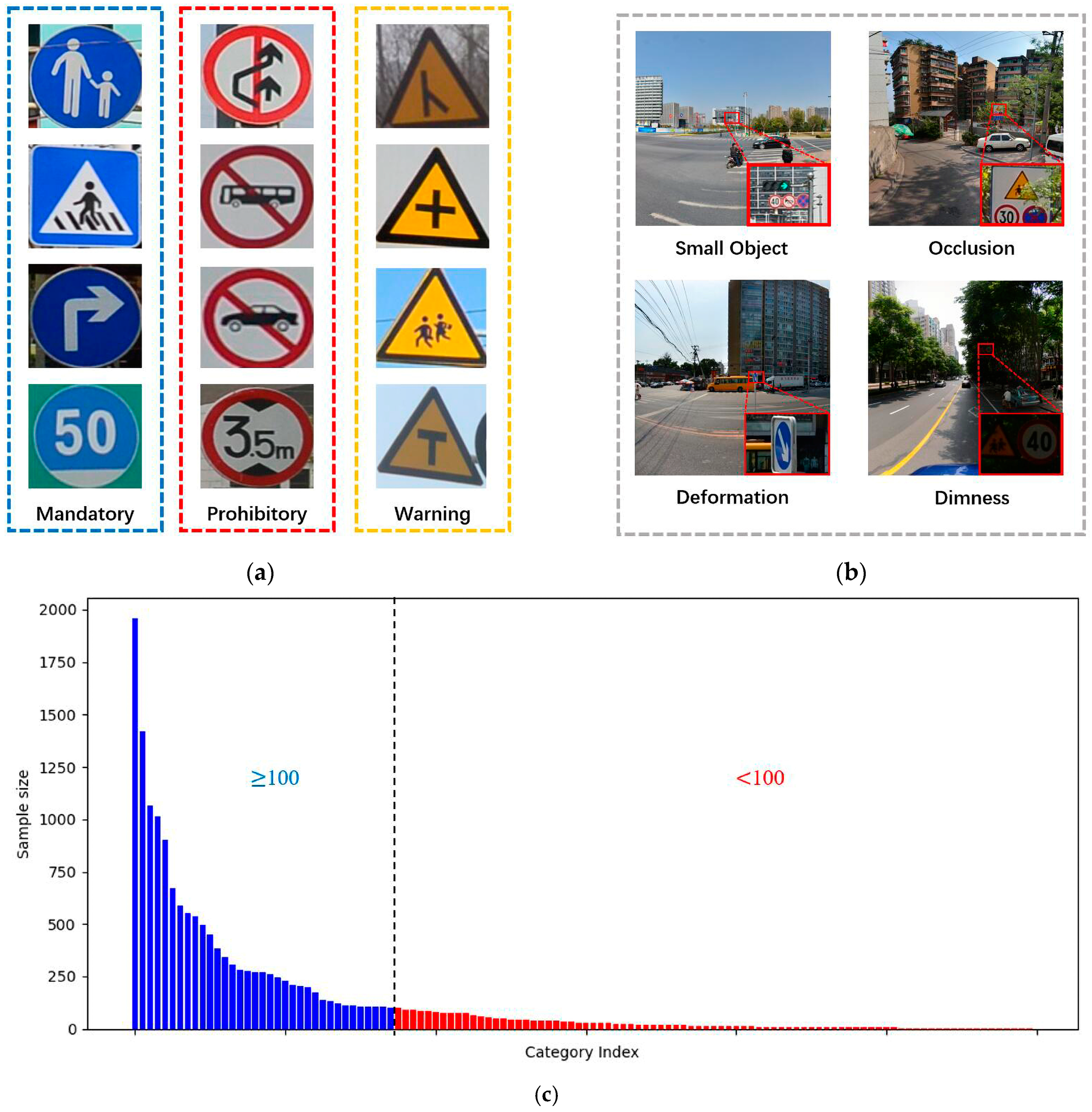
Figure 1a, traffic signs are typically classified into three types: warning, prohibitory, and mandatory. Each of these categories can be further subdivided to provide a more detailed range of guidance information, such as road types, prohibitions, speed limits, and height limits. Traffic sign detection and recognition require the precise location and classification of traffic signs in the vehicle image.
Traffic signs are designed with distinct shapes such as squares, circles, and triangles, as well as distinct red, yellow, and blue colors to highlight the sign. Traditional detection and recognition methods are thus achieved by designing manual feature descriptors for traffic sign detection and recognition. The use of sliding windows to find high-probability regions in an image containing traffic signs is one example [
1]. Researchers have also attempted to determine adaptive segmentation thresholds for traffic sign extraction and classification by computing histograms of images [
2,
3]. Color space has also been used, for example, in segmentation in HSV [
4]. Researchers extracted SURF feature points from signs and used corroding images to match them [
5]. In some studies, more complex feature descriptors, such as coarse localization of signs based on the Hough transform [
6], were used for sign extraction. Traditional digital morphology-based methods typically necessitate clear images with high-resolution signs and no anomalies to interfere, making them difficult to apply in complex real-world scenarios.
Researchers added machine learning algorithms for refinement based on digital morphology to improve the model’s robustness. Traditional HOG features were combined with SVM for traffic sign detection and classification [
7,
8]. The researchers attempted to segment the images based on color features and then used SVM to implement classification on the segmented regions [
9,
10,
11]. Since many traffic signs are circular in shape, the researchers used the circular Hough transform to detect the signs and then classified them using SVM [
12,
13]. Although the support vector machine improves detection and recognition accuracy, it is still heavily reliant on manual features. As a result, the improved model, while capable of more accurate and detailed classification, struggles to deal with the anomalies depicted in
Figure 1b.
Object detection algorithms based on convolutional neural networks have become a better choice for academics due to the extensive use of high-performance computer systems. However, smaller traffic signs are difficult to detect and classify accurately as the detailed features of small targets are difficult to transfer to the deeper feature maps. Some researchers have used image super-resolution algorithms to enhance the detection of small targets [
14,
15]. Since attention mechanisms can drive the network to focus more on channel and spatial feature acquisition, adding attention mechanisms to the model can also improve the model’s ability to extract semantic features [
16,
17,
18,
19,
20].
From different viewpoints, traffic signs produce images of varying scales, and changes in scale can also affect detector performance. Researchers attempted to incorporate deformable convolution into the network, which can adjust the perceptual field adaptively [
19,
21,
22]. Because the backbone generates feature maps of varying sizes during layer-by-layer downsampling, some researchers have fused feature information from various scales by constructing feature pyramids in order to improve the model’s extraction of multi-scale features [
22,
23,
24,
25,
26,
27,
28,
29,
30].
Some researchers have improved model performance without changing the detector by using pre-processing techniques, such as image enhancement based on probabilistic models [
31], highlighting edge features of traffic signs [
32], and enhancing the hue of dark areas of images [
33]. In addition, on-board cameras typically take high-resolution images for sensing the vehicle’s surroundings but increase the search range for traffic signs. Therefore, an attempt has been made in some studies to construct a coarse-to-fine framework, which is used to reduce computational costs and improve model performance [
34,
35,
36]. Background information is frequently ignored, but some researchers have improved model accuracy by using background detail features of neighboring signs [
37,
38]. In addition, spiking neural networks (SNN) are used to improve existing traffic sign detection and recognition algorithms [
39,
40,
41], which can extract time-related features and have higher computational efficiency on hardware platforms.
To obtain accurate indication information, we must classify traffic signs down to the smallest category, which requires the algorithm to accurately identify up to several hundred sign categories. As shown in
Figure 1c, there is a great difference in sample size between the traffic sign classes. This will result in classes with larger sample sizes having better classification accuracy, while classes with sparse samples perform poorly [
42]. Existing studies usually only identify traffic signs according to three categories: prohibited, warning, and mandatory, or remove categories with a sample size of less than 100. However, each category of traffic sign is designed to convey important guidance information. Therefore, the detection and recognition of traffic signs need to be implemented in as comprehensive a range of categories as possible.
On-board cameras can continuously capture traffic signs, but most existing studies only use information from a single image. Missed detections or misclassifications due to anomalies such as occlusion and deformation are typically present in only a few frames, but incorrect detection of a single sign can also pose a serious hazard, negatively impacting the environment, infrastructure, and human life. Some researchers have attempted to improve detector performance using image sequences in previous studies [
43,
44,
45,
46], but this often necessitates an additional training process and consumes more computational resources. Meanwhile, successive detections can result in redundant results.
In general, the main contributions of this paper are summarized as follows:
- (1)
We propose a hierarchical classification model (HCM) based on the natural distribution characteristics of traffic signs, which is used for the classification of traffic signs in full classes. Meanwhile, the HCM significantly reduces the degree of imbalance between classes without changing the sample size.
- (2)
To deal with missing or misleading information caused by anomalies, this study designed a multi-frame information aggregation module (MIM) to extract the detection sequence of traffic signs, which is based on the embedding generated by the HCM. The temporal sequence of detection information can deal with the shortcomings of a single image, reducing false detections caused by anomalies.
- (3)
We validated our method using two open-source datasets, TT100K and ONCE. The HCM-improved YOLOv5 achieves a mAP of 79.0 in full classes, exceeding existing state-of-the-art methods. Experiments using ONCE show that MIM further improves the performance of the model by integrating multi-frame information.
2. Methods
The image sequence
captured by the on-board camera is used as input in this work, and we need to detect and recognize traffic signs for each frame. Specifically, we need to detect the bounding box
of each traffic sign and recognize the specific category
. The central coordinates, width, and length of the bounding box are noted as
,
,
, and
, respectively.
In conclusion, our work can be summarized as Equation (1).
and
in the formula are the set of traffic sign categories and the set of time, respectively.
is the number of traffic signs in the image
.
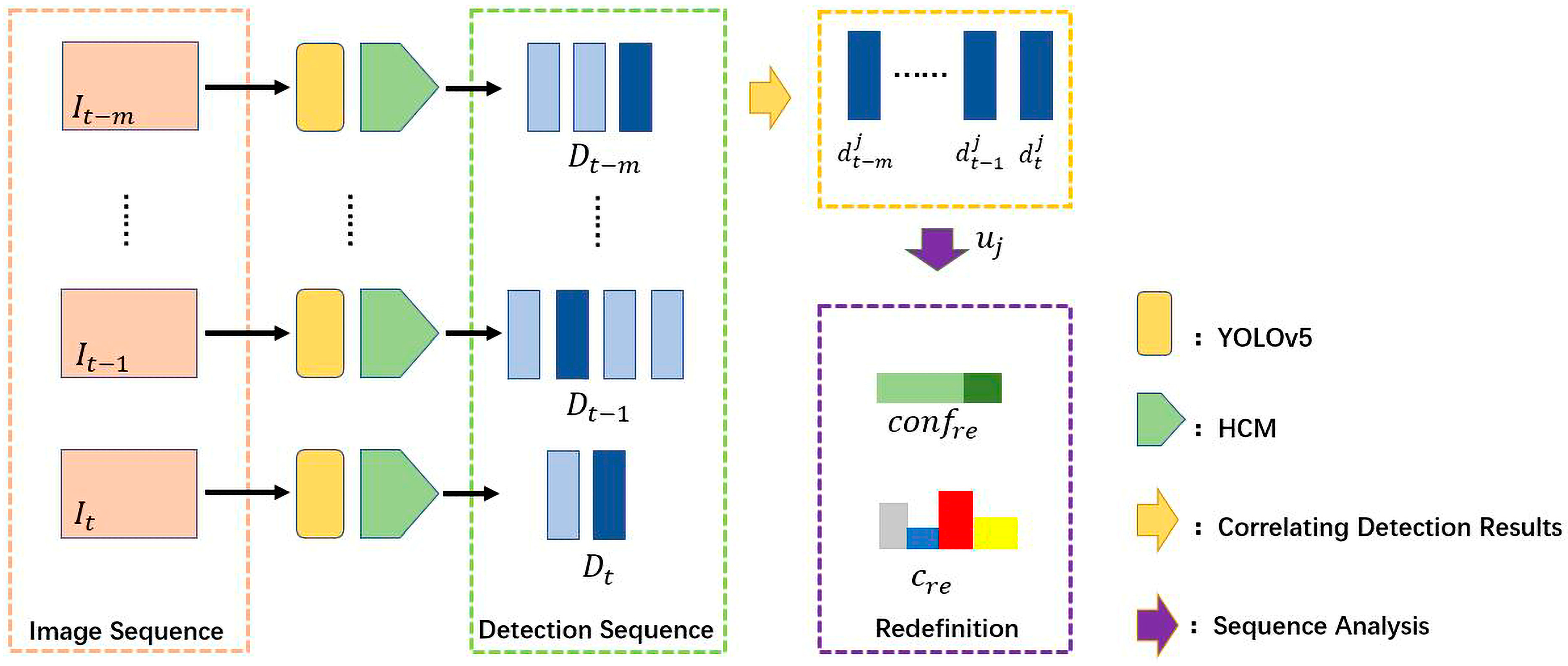
Figure 2 illustrates the overall framework of our method. While the vehicle moves, the on-board camera catches street scenes, creating a temporal sequence of photos
. The processing steps of our algorithm can be summarized as follows:
Step 1: We use the previous frames as reference frame set for a given image inside .
Step 2: Based on the image and all reference frames, YOLOv5 generates a number of candidate regions through detection.
Step 3: The hierarchical classification module (HCM) implements the specific classification of candidate areas.
Step 4: Based on the embedding extracted by the HCM, the multi-frame information integration module (MIM) searches for associated boxes in reference frames.
Step 5: MIM analyzes the detection sequences generated by the association operation, which is used for category and confidence redefinition.
2.1. Detector
Object detection is used to locate targets in an image and perform category recognition. Yet, because of small objects, large-scale changes, and long-tailed distributions, it is challenging to accomplish robust detection by merely applying a generic object detection algorithm. At the same time, the algorithm’s inference speed is a crucial assessment criterion in order to interpret sign information in a timely manner on rapidly moving cars.
Object detection can be divided into two categories, depending on the framework: one-stage and two-stage. Object detection algorithms with two stages generate regional proposals first, then classify each proposed region. A considerable number of regions of interest are generated via region proposals. For example, R-CNN [
47] creates approximately 2000 proposed regions in each input image. Because each proposed region needs independent feature extraction and classification, two-stage object detection necessitates considerable inference space and time costs.
In contrast to the classification and regression of proposed regions, one-stage object detection typically divides the image into a number of grids, each containing a number of a priori boxes. Following that, based on the feature maps provided by the backbone network, the algorithm predicts the position and class of objects within each grid [
48]. Compared to the two-stage algorithm, the one-stage object detection uses a more direct global regression and classification. The one-stage framework allows for fast inference as there are not a large number of candidate regions to be computed independently.
In addition to the speed of inference, the accuracy of the model is an important consideration. The scale fluctuations of traffic signs and small objects result in generic object detection methods that are frequently hard to recognize robustly. MS-COCO [
49] defines objects with an area of fewer than 32 × 32 pixels as small objects. The sparse appearance of small objects makes it difficult for the algorithm to distinguish between background and object, and it also places higher challenges on the model’s detection accuracy [
50]. During the feature extraction process, the backbone network can generate feature maps of different sizes to represent information at various scales. Shallow feature maps contain more detailed spatial features, while deeper feature maps represent more abstract semantic features. To address the performance decrease caused by scale factors, researchers designed the feature pyramid network (FPN) for fusing feature information at multiple scales by concatenating or summing elements between feature maps.
For reasons of inference speed and detection accuracy, the detection and recognition of traffic signs require a one-stage object detection algorithm that adapts to the multi-scale variation. Following comparison, YOLOv5 is selected as the detector in this research. As a member of the yolo series of object detection algorithms, YOLOv5 not only inherits the conventional quick detection capabilities but also applies a number of tactics to mitigate the detrimental impacts of scale variation and small objects. Specifically, benefiting from a unique residual structure and spatial pyramidal pooling, YOLOv5 has excellent multi-scale feature extraction capabilities, which help to extract traffic sign features at different distances. The creation of a bi-directional feature pyramid structure improves information transfer across features at different scales and the model’s retention of detailed features in the image. At the same time, traffic signs have distinct shapes and color qualities that set them out from the background, so YOLOv5 can be used to precisely locate traffic signs in an image.
In the real world, traffic signs suffer from a sample imbalance between categories, which has a direct impact on the dataset. Although object detection algorithms contain both localization and classification capabilities, the long-tailed distribution of traffic signs frequently results in significant a reduction in the algorithm’s classification performance. YOLOv5 achieves multi-classification in the head by modifying the feature map size, but the imbalanced distribution of data has a substantial impact on the model’s detection and classification performance. Therefore, YOLOv5 is not suitable for both the detection and recognition of traffic signs, but traffic sign localization can be effectively solved by using a single classification that distinguishes the traffic signs from the background.
Given the input image sequence , we will utilize YOLOv5 to locate the traffic signs in the image. For one of the images , the detector will obtain bounding boxes and the corresponding confidence, denoted as . The bounding box is represented by the term in the equation, which contains the length, width, and centroid coordinates of the box, while the other component is used to describe the confidence of the detection, . By processing the entire image sequence with YOLOv5, we can obtain a detection sequence .
2.2. Hierarchical Classification Model
Although YOLOv5 as a detector can effectively address the problem of localizing traffic signs in photos, robust classification is difficult to obtain. The difficulty in categorization is due to the fact that there are hundreds of kinds of traffic signs and that the distribution of samples is significantly imbalanced. In general, YOLOv5 needs a new classification module that is able to achieve accurate classification for all classes in the case of long-tailed distributions. Moreover, as there is often more than one traffic sign in an image, the classification model should avoid using complex structural designs, which can lead to long processing times for a single image.
The dataset of traffic signs generally suffers from an uneven distribution of samples, which reflects the distribution in realistic scenarios. The mandatory category of signs, which is typically used to guide lane information, has a large sample size, while the warning category of signs has an extremely limited sample size. Despite the fact that there are hundreds of traffic sign classifications, a few common categories account for the vast majority of samples in the dataset. Based on the sample size, we divided the traffic sign categories in TT100K into three categories: large, medium, and small. Categories with fewer than 10 samples were labeled as small, those with more than 50 samples were labeled as large, and the remaining categories were labeled as medium.
Table 1 depicts the percentage of sample size and the percentage of number of categories for these three types of signs. The category with a large sample size accounts for only 20.6% of all categories but has 43.9% of the sample size. In contrast, the low sample size category accounts for more than half of all categories but has a sample size of only 12.2%.
When faced with imbalanced sample sizes, previous research has often used either under-sampling or oversampling to balance the sample size. Both strategies are data-level approaches, but under-sampling yields less data for model training, whereas oversampling lengthens training time and may result in model overfitting [
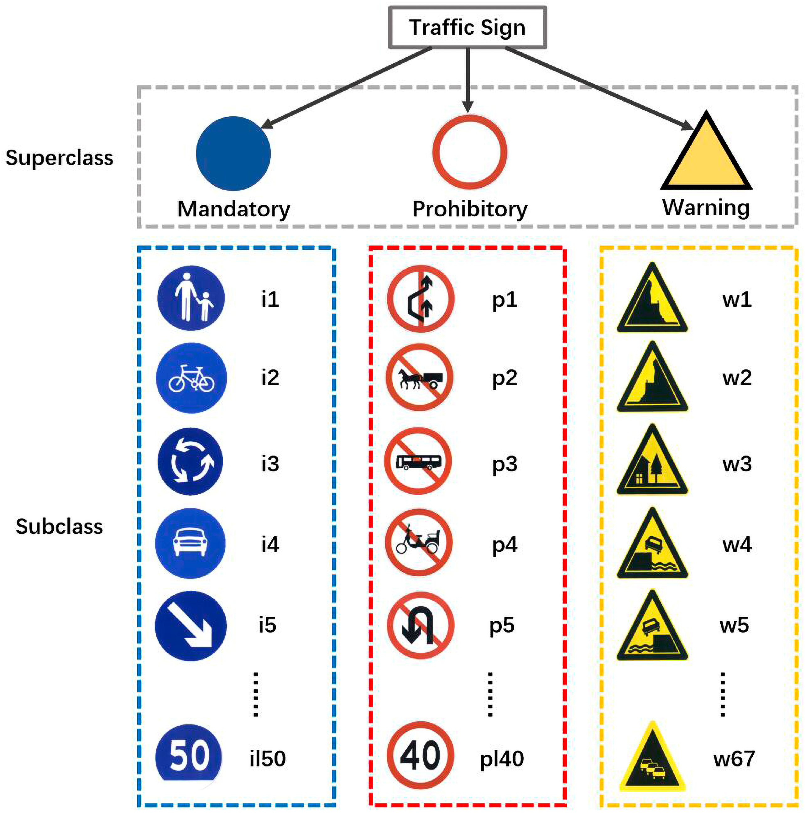
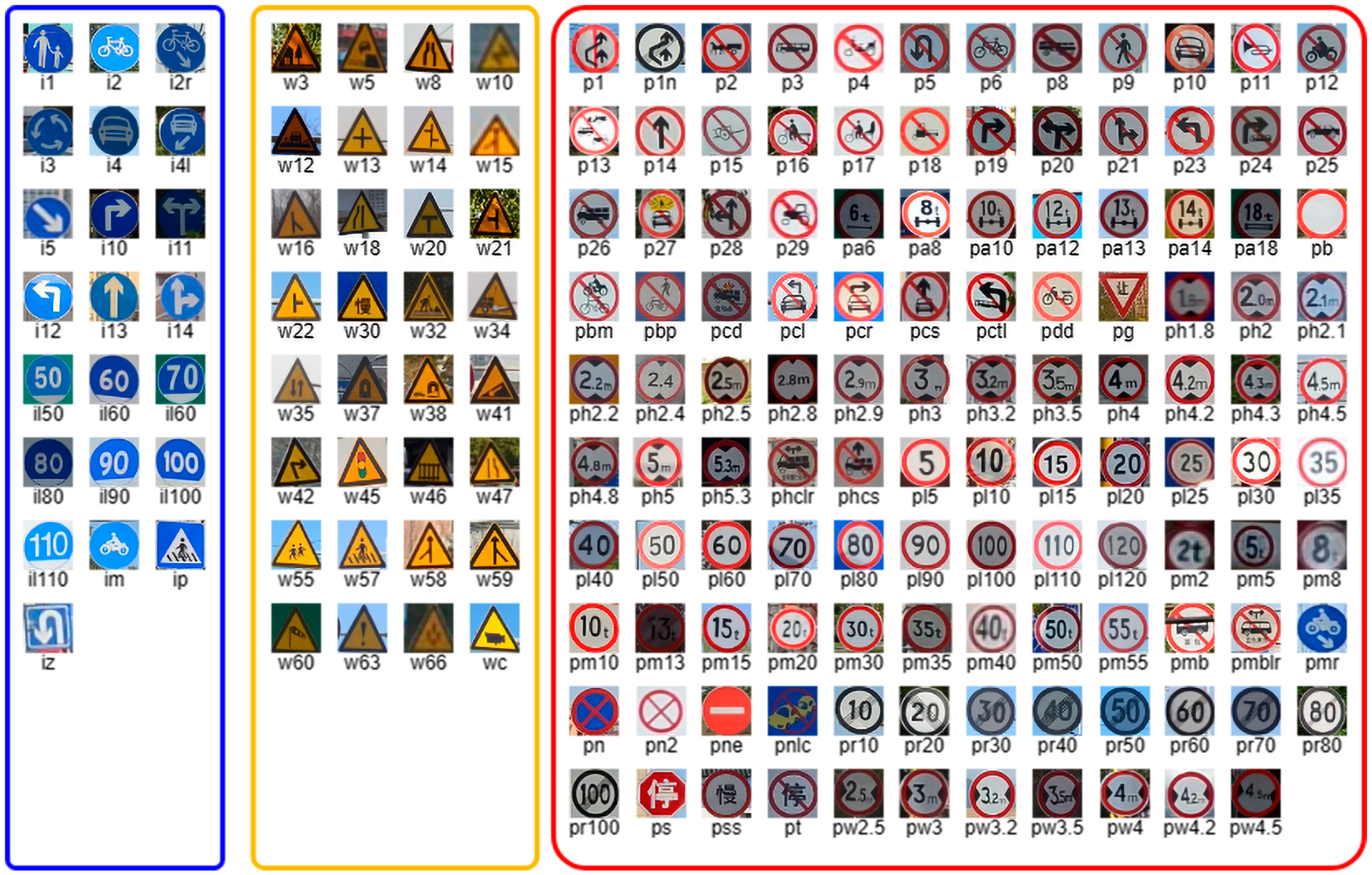
42]. Unlike data augmentation, we employ a grouping strategy to classify traffic sign categories. Traffic signs are classified into three superclasses: warning, prohibitory, and mandatory, with a number of specialized subclasses within each superclass. As illustrated in
Figure 3, the superclasses range significantly in color and shape. For example, prohibitory signs have a red circular border, but warning signs have triangular and yellow features. This significant difference in features makes it easy for the classification algorithm to achieve better classification accuracy on the superclasses. The difficulty in classification is to precisely identify subclasses with a long-tailed distribution. However, we discovered that the majority of the mandatory signs are seen in classes with a large sample size, whereas the warning signs are typically found in classes with a small sample size. While the overall sample distribution exhibits a significant long-tailed distribution, the difference in sample size between subclasses within a superclass is much smaller. Thus, grouping can improve the overall performance of the classification model by reducing the degree of imbalance without changing the sample size.
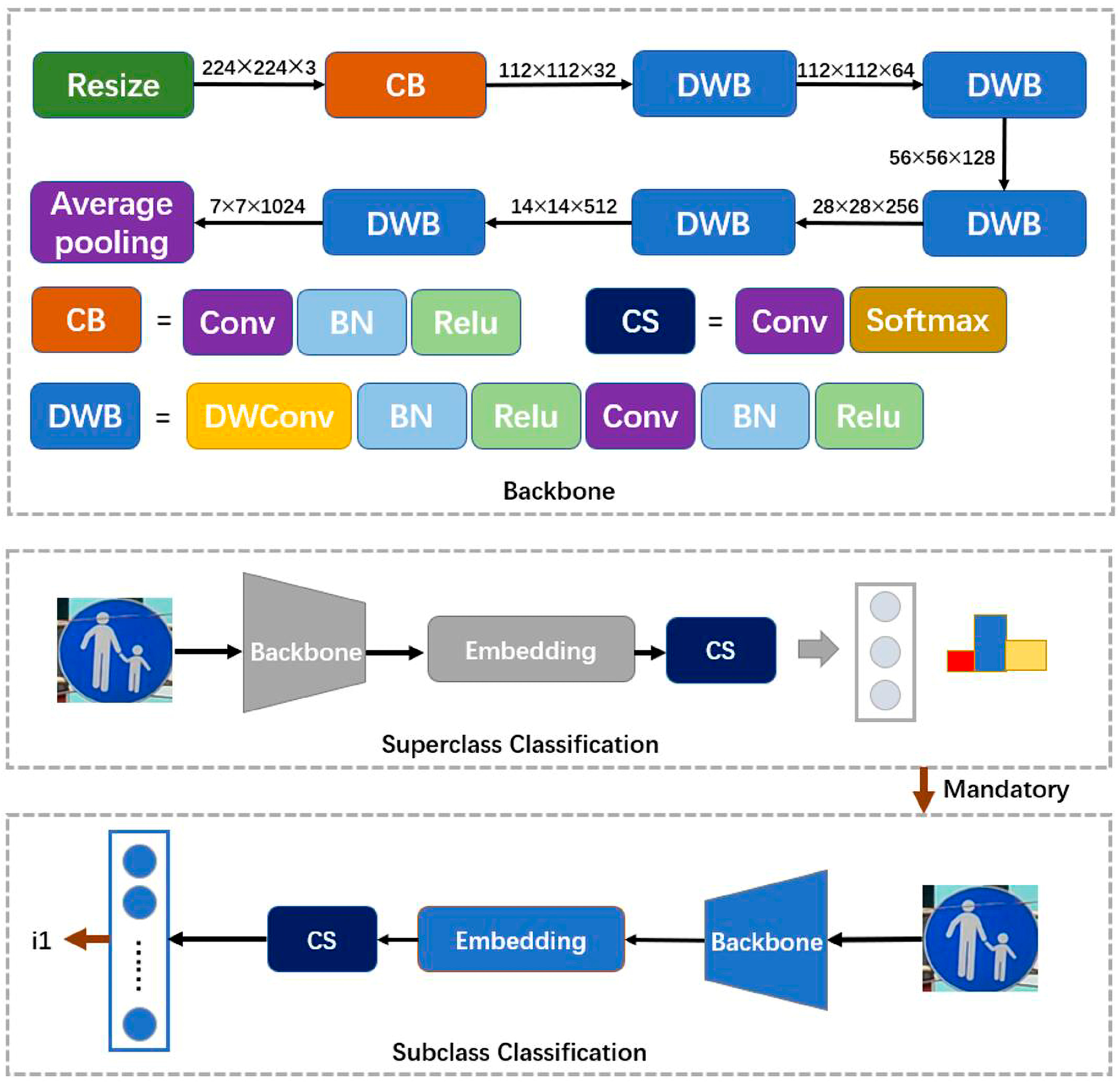
Based on the grouping results, a lightweight hierarchical classification module (HCM) was built and used to identify superclasses and subclasses. Although classifiers tailored to each superclass can be created, this typically slows down inference. Therefore, the HCM is made up of four structurally identical sub-networks, one of which serves as a superclass classifier and the other three for subclass recognition within the superclass. Each subnetwork can be divided into two parts: the backbone and the classification component (CS). The extraction of deep semantic features is required for a number of candidate regions provided by YOLOv5. We built a lightweight backbone based on MobileNet to accomplish quick feature extraction. The input images were initially rescaled to 224 × 224 × 3. Following that, we extracted features using lightweight convolutional components. To extract features, we then constantly downsample the input image based on the convolutional component. This procedure is as follows: given a candidate region , the backbone generates a high-dimensional embedding through progressive downsampling, .
Following traffic sign feature extraction, we combine the convolution and softmax functions to generate a classification component . Convolution is used for classification rather than fully connected layers because the number of parameters in fully connected layers increases dramatically as the number of classes to be classified increases, increasing space and time consumption. We first determine the convolution kernel depending on the number of categories, then change the feature embedding to a feature map of the desired size using convolution operations, and lastly use the softmax function to produce the classification result , or .
As shown in
Figure 4, HCM begins prediction by identifying superclasses, following which the relevant subclass classifier is chosen for a specific classification. Simultaneously, there are model training requirements. We adjust the number of classifications by changing the convolution kernel parameter
in the classification component
. Take the superclass classifier as an example, where the classification component generates a feature map of size 1 × 3 for the identification of the three superclasses. After completing the structural design of the HCM, we use a cross-entropy loss function for model training. The
and
in Equation (2) denote the ground truth and predicted value, respectively.
For one of the frames
, we first extract all the candidate regions from the detection result
. Afterwards, the HCM identifies each candidate region
independently. Following the classification results, we supplement
with specific categories and embeddings. After processing by HCM,
can be expressed by Equation (3).
2.3. Multi-Frame Information Integration Module
Although the combination of YOLOv5 and HCM can mitigate the detrimental effects of scale variation and long-tailed distribution, occlusion and deformation issues in real-world scenarios can still result in missed detections and misclassification. However, we discovered that traffic signs are typically captured multiple times by the in-vehicle camera, and the majority of the detection and recognition results are correct, while occlusion and deformation are only present in a few frames. To use information from multiple frames, the multi-frame information integration module (MIM) first correlates detection results between frames using the embedding generated by the HCM and then uses the output from previous frames to improve model performance. The accumulation of detection results from multiple frames can compensate for a single frame’s lack of information, reducing the number of missed detections and misclassifications. Besides that, comparing inter-frame detection outputs can be used to eliminate redundant results produced during the continuous detection state.
2.3.1. Correlating Detection Results
Before association, we need to filter the image sequence. The previous
frames
in image sequence
are utilized as a reference frame set for a given picture
, where the number of
is connected to the number of times the traffic sign appears in the image sequence. Following that, MIM needs to find associated detections in the reference frame, which necessitates applying high-dimensional embeddings. Although several methods for obtaining embedding have been proposed in previous works [
51,
52], embeddings generated using HCM can avoid additional computational resource consumption while achieving association.
The HCM generates a high-dimensional embedding of traffic signs, which is useful for distinguishing between different types of traffic signs but difficult to differentiate between instances of the same type. To that purpose, we extract the feature embedding
and the centroid coordinates of the bounding box, which are used for the traffic sign’s distinguishing feature set
,
. Following that, we created a function
to determine the similarity between two traffic signs. Specifically, we first designed
, a function for quantifying the similarity of embeddings based on cosine similarity. Equation (4) can be used to calculate the corresponding embedding similarity given two distinguishing features,
and
.
Following that, we created
, a similarity computation function based on the Euclidean distance. Due to the large range of the Euclidean distance,
needs to perform a normalizing operation, as indicated in Equation (7).
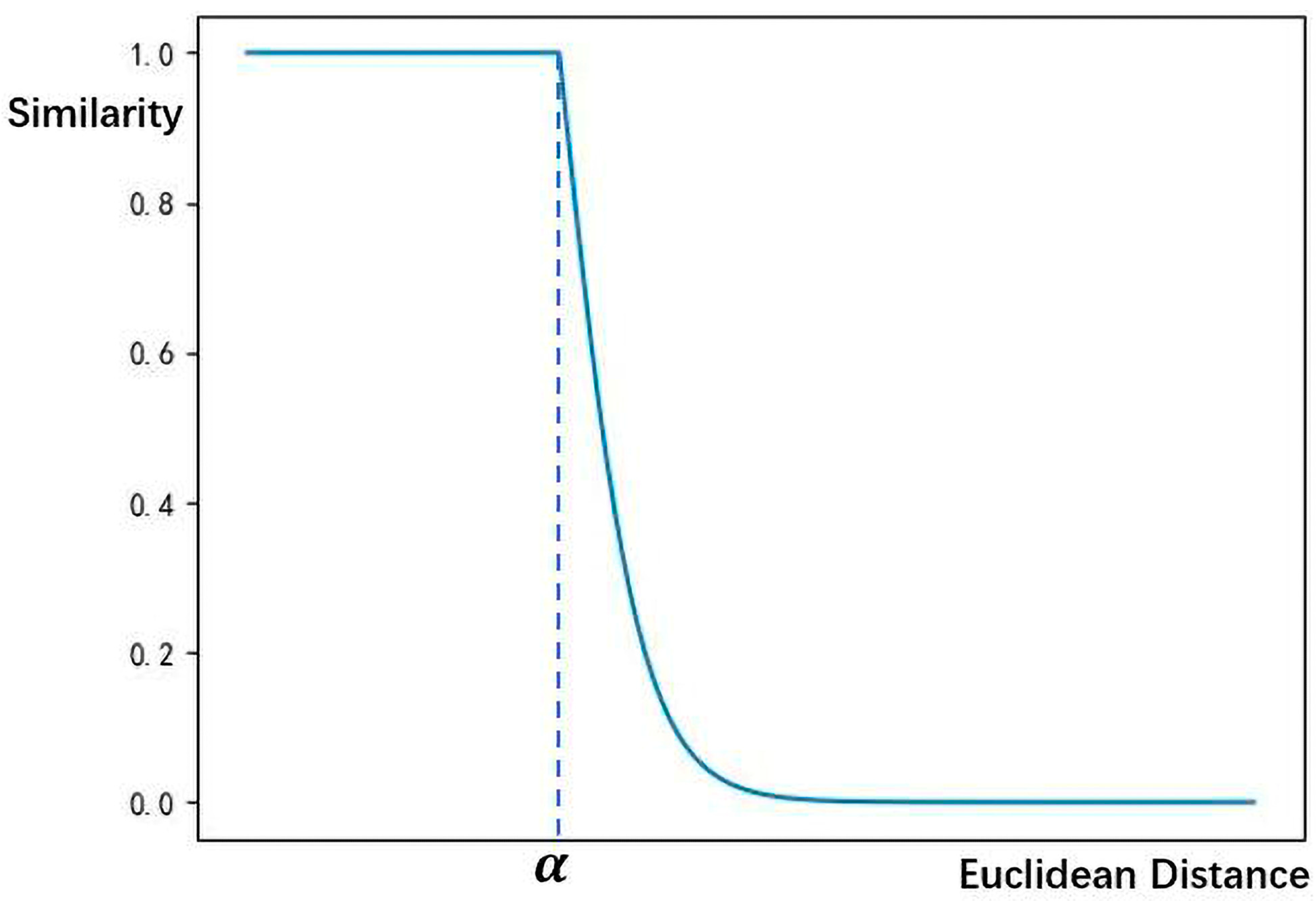
To enable an adjustable normalization calculation of the Euclidean distance, a hyperparameter
is set in
to reflect the centroid offset of the traffic sign instance between frames. As shown in
Figure 5, the computed similarity is greatest when the Euclidean distance is less than
. We also utilize another hyperparameter
to alter the Euclidean distance range of interest. Lastly, Equation (8) depicts the weighted sum integration of similarity information from embedding and Euclidean distance.
Since the function
achieves result association mostly through embedding, the weight parameters should be set so that
is greater than
.
Figure 6 shows two examples of how similarity information from both aspects can be used to distinguish among different traffic signs. For a distinguishing feature
in current frame
,
, the similarity is calculated based on the function
for the results in the reference frame
. As stated in Equation (9), the procedure will produce a set of similarity scores. Afterwards, we extracted the maximum similarity scores
and the corresponding distinguishing feature
based on Equations (10) and (11), respectively.
If exceeds the similarity threshold , the detection result corresponding to becomes the association result in , which is denoted as . Similarly, we seek association results that satisfy the requirements in all reference frames. After that, the detection result is included to generate the sequence of detection results . Lastly, for all traffic signs in the current frame , we can extract the set of detection results .
2.3.2. Sequence Analysis
In real-world circumstances, traffic signs have anomalies such as occlusion and deformation, which can lead to false detection or misclassification by the detector. Fundamentally, the anomalies cause the image’s information to be absent or deceptive. As anomalies are typically present in only a few frames, the lack of information in a single image can be compensated for by employing several detections, which can enhance the model’s performance even further.
Based on the findings of the preceding analysis, MIM redefines categories and confidences based on the sequence of detection results, as illustrated in
Figure 7. To count the confidence of category
in the sequence, we construct a statistical function
, denoted as Equation (12). After that, Equation (13) is used to calculate the category with the highest cumulative confidence in the sequence
. Finally, the category with the highest confidence becomes the redefinition category
, while the redefinition confidence
is calculated by Equation (14).
To eliminate detection results with poor confidence, a hyperparameter
is applied. When the confidence
is greater than
, the categories and confidence levels in
are replaced by the redefined results. The final result can be expressed by Equation (15). Based on the same process, we redefine all detection results in current frame
.
Overall, by integrating information from multiple detections, sequence analysis mitigates the unfavorable impact of abnormalities. While the majority of the results in the detection sequence are correct, the redefinition results from sequence analysis can correct for a small number of classification errors. Simultaneously, deformation might occur at viewpoints near traffic signs, which usually results in low confidence in the results. When employing multiple detections, the confidence level can be enhanced by leveraging high-confidence information from previous results, resulting in fewer missed detections.
3. Results
3.1. Dataset
We deal with specific kinds of traffic signs in this study; however, a portion of the traffic sign datasets are only labeled with three categories: warning, prohibitory, and mandatory [
53,
54]. In contrast, TT100K [
55] and ONCE [
56] are better candidates because their annotation information is more detailed.
TT100K contains 10,000 images with a resolution of 2048 × 2048. At the same time, the data annotation is further refined into 232 specific categories, as shown in
Figure 8. Existing studies typically remove categories with a sample size of less than 100 [
19,
57,
58,
59,
60], but we use the full traffic sign category for model training and testing. On the other hand, the ONCE dataset is an autonomous driving dataset with millions of scenes. The images in the dataset were selected from 144 h of on-board camera video, taken under different lighting and weather conditions. In order to use the temporal image data in ONCE, we annotated the ONCE test set similarly to TT100K. After removing the night data, the test set contains 13,268 time-series images with a resolution of 1920 × 1020.
3.2. Metrics
The experiment uses precision, recall, and
F1 score as metrics to evaluate the overall performance of the detector, as indicated in Equations (16)–(18).
F1 is the arithmetic mean of precision and recall.
where true positives (
TP) are the number of samples that are actually positive and classified as positive by the classifier; false positives (
FP) are the number of samples that are actually negative but classified as positive by the classifier; and false negatives (
FN) are the number of samples that are actually positive but classified as negative by the classifier.
Certain evaluation criteria, such as precision, have the potential to mislead researchers [
42]. When a long-tailed distribution exists, high scores may mistakenly represent good performance. As a consequence, we use
mAP to further evaluate the model’s performance. As indicated in Equation (19),
mAP is the average of each category’s mean average precision, i.e., the average precision of all categories divided by the number of categories. This paper uses a fixed intersection-over-union (IoU) value of 0.5 for computing
mAP.
3.3. General Detector
Although newer versions of the YOLO model have been proposed, YOLOv5 still has an advantage in the detection of traffic signs. To prove this point, the stable YOLOv7 was chosen for comparison. Based on the TT100K dataset, we calculated the overall metrics for YOLOv5, YOLOv7_l, and YOLOv7_x on the single classification detection task, as shown in
Table 2.
YOLOv7 outperformed YOLOv5 in terms of AP; however, when inferring, the detection algorithm needed to determine the final output based on a confidence threshold. Based on the same confidence threshold of 0.5, YOLOv7_l outperforms YOLOv5 in terms of precision but is lower than YOLOv5 in terms of recall and F1 score. Therefore, YOLOv5 is more suitable for traffic sign detection than YOLOv7.
We tested performance using SSD, Faster RCNN, CenterNet, and YOLOv5 as baselines, which are derived from diverse architectures of target detection algorithms, to indicate that generic object detection algorithms are challenging to apply to the detection and recognition of traffic signs. SSD and YOLOv5 are typical one-stage models; Faster RCNN is a two-stage algorithm; and CenterNet is well known for its unique anchor-free architecture. Since TT100K has detailed category information, all baselines are trained using the training set of TT100K until the model converges.
First, we recorded the overall metrics of the baselines on the TT100K test set in
Table 3. The results show that CenterNet and YOLOv5, which have been proposed in recent years, outperformed SSD and Faster RCNN.
Figure 9 compares the detection results of the baselines to further analyze the reasons for the difference in performance. The traffic signs in the red boxes are typical small objects in this case, and the signs in the yellow and blue regions show deformations due to the viewpoint. According to the results, SSD and Faster RCNN, which lack the ability to fuse multi-scale information, have a high percentage of missed detections on small objects, whereas CenterNet and YOLOv5, which use a feature pyramid structure, detect much more small-object traffic signs.
At the same time, this example reflects the negative impact of the long-tailed distribution on the detector. Specifically, the traffic sign in the yellow area has some deformation, but the sample size of the corresponding category is sufficient. In contrast, the corresponding category in the blue region has a much smaller sample size. Although the traffic signs in the yellow and blue areas have similar deformations, the difference in sample size leads to completely different results.
The overall metrics do not accurately represent the model’s performance across categories with varied sample sizes. As a result, we first compute the average precision of the baseline across all categories. After that, we calculated
mAP in accordance with the difference in sample size, which is shown in
Table 4.
The results show that there is a significant difference in accuracy between the categories with an adequate sample size and those with fewer samples. YOLOv5 has a higher mAP in categories with sufficient sample size. However, for the category with fewer samples, the gap between baselines is substantially lower. As a result, YOLOv5 is not suitable for combining detection and multi-classification tasks for objects having a long-tailed distribution, such as traffic signs.
The photos in TT100K are often taken in bright light, and the majority of the samples are small. ONCE, on the other hand, records photographs in a variety of weather conditions, such as sunny, rainy, and cloudy days, but with a lower proportion of small objects than TT100K. We used the same strategy to compute the metrics for the ONCE baseline method and recorded them in
Table 5.
The test results on ONCE are basically unchanged, with the exception that Faster RCNN performs substantially better than TT100K on ONCE, showing that the small object is the primary cause for Faster RCNN’s limited performance.
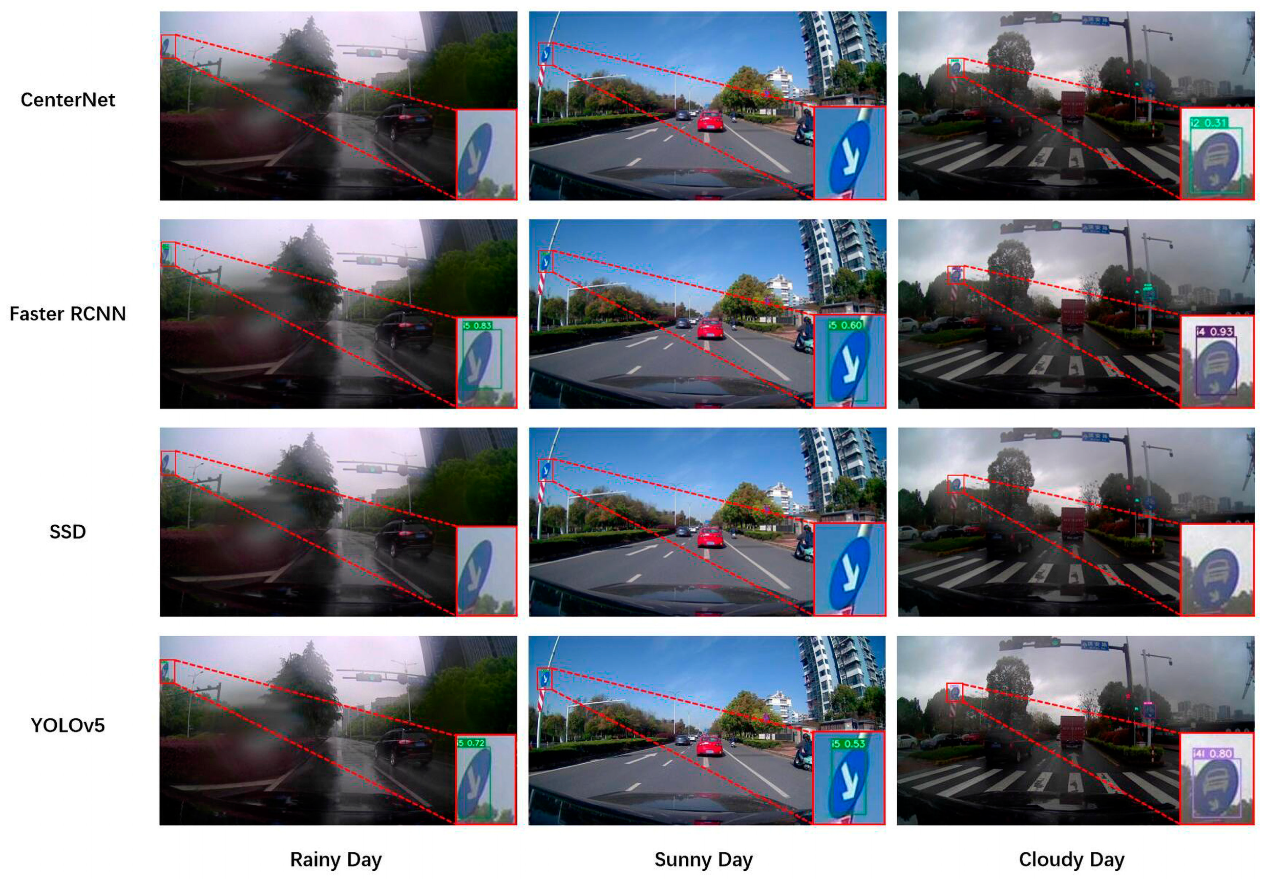
Figure 10 shows detection in three types of weather to illustrate the impact of weather on model performance. The images in the sunny environment are clear, but those in the cloudy and rainy surroundings are substantially dimmer. The effect of environmental elements is also represented in the baseline results; for example, cloudy and rainy conditions result in more missed detections or misclassifications. It was also discovered that, while Faster RCNN performed well overall, it lacked localization precision.
Based on this, we calculated the
mAP of the baseline for categories with varying sample sizes, as shown in
Table 6. The results of the tests show that the Faster RCNN outperforms SSD and CenterNet in the less-sample category. On cloudy days, the Faster RCNN performs better as a two-stage object detection method.
3.4. HCM-Based Method
This section evaluates the performance of the HCM-improved model to validate the efficacy of our method. The HCM-improved YOLOv5 is labeled as YOLOv5-HC. In the training process, the input image resolution was adjusted from 2048 × 2048 to 640 × 640 after downsampling. The initial learning rate of the model was set to 0.001, and Adam was used as the optimizer for the network training.
Since HCM is an image classification model, the TT100K training set must be cropped based on the annotations to obtain picture samples of traffic signs. HCM is composed of four separate sub-networks, one of which produces a feature map of size three for superclass recognition and is trained using all of the data in the training set. The remaining subnetworks are used for the three superclasses’ subclass identification, and each subnetwork is trained using data from the corresponding superclass. The subnetwork for mandatory sign recognition, in particular, generates a feature map of dimension 22, which corresponds to the 22 mandatory traffic sign subclasses. Similarly, to accommodate the specific number of subclasses, the sub-networks used to recognize prohibitory and warning signs will build feature maps of dimensions 119 and 32, respectively.
During the training of each sub-network, the input image was resized to 224 × 224 while Adam was set as the network’s optimizer. The network training was divided into two sections. First, we freeze the backbone weights and set the learning rate at 1e-3. Following that, training with 20 epochs is used to change the weights of the convolutional layer in the classification component. The backbone weights are unfrozen in the second stage, and the learning rate is decreased to 1 × 10⁻⁴. To finish fine-tuning the weights, the model is trained for 30 epochs.
After finishing the training, we recorded the overall metrics of YOLOv5-HC on the TT100K test set in
Table 7. The results show that YOLOv5-HC outperformed YOLOv5 by 11.16%, 14.36%, and 12.64 points in precision, recall, and
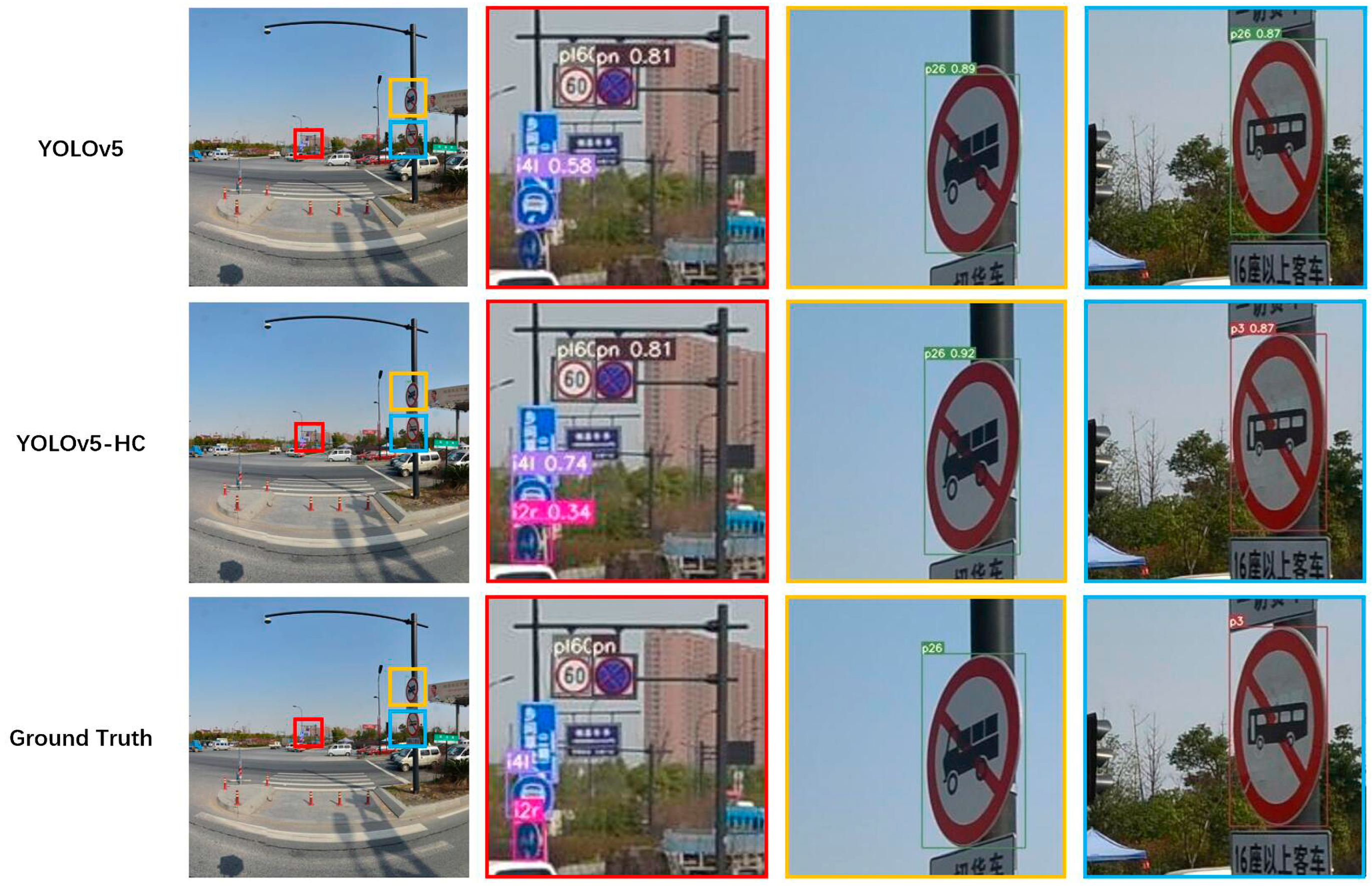
F1 score, respectively. YOLOv5-HC discovered the most complicated small object i2r in the red region shown in
Figure 11. Meanwhile, only YOLOv5-HC correctly classified the few-sample category sign in the blue region.
We computed
mAP for YOLOv5-HC on categories with varied sample sizes in order to explicitly analyze the performance of HCM on fewer sample categories, which is recorded in
Table 8. YOLOv5-HC improves accuracy across all categories. As the sample size reduces, the degree of performance improvement of HCM on YOLOv5 increases. In addition, we compared YOLOv5-HC with related methods in full classes, as shown in
Table 9. Compared to the state-of-the-art model, YOLOv5-HC has a 7.1% improvement in
mAP across all categories. Furthermore, our method has fewer model parameters.
As traffic sign identification and recognition require rapid perception information, the model’s inference speed is also an important metric. We used Nvidia 2080ti to calculate the inference speed of YOLOv5 and YOLOv5-HC, as shown in
Table 7. Despite the fact that the use of HCM increased the inference time, YOLOv5-HC still achieves an inference speed of 22.7 FPS. In terms of the balance between model accuracy and inference speed, we want to improve the accuracy of the model as much as possible while satisfying the real-time condition. Taking the autonomous driving dataset ONCE as an example, the data is sampled at a frequency of 10 FPS, so we consider that the inference speed of 22.7 FPS satisfies the real-time requirement.
3.5. MIM-Based Method
Unlike TT100K, the data in ONCE are organized temporally. While MIM is intended to be a training-free post-processing framework, we still use the model that completed the training in the previous section, but test the detector on the ONCE test set based on multiple frames of images. The MIM-improved YOLOv5-HC is labeled YOLOv5-HM.
The pre-requisite for implementing multi-image processing is to determine the number of reference frames . Based on the temporal information of the current frame, the MIM selects images before the current frame as a reference frame set. A temporal sequence that is too long would result in computational redundancy. On the other hand, a temporal sequence that is too short will miss some of the essential sign-detection information. By analyzing the images in ONCE, we set .
The MIM module first needs to correlate the detection results in the image sequence, where a number of hyperparameters need to be set. For ONCE, both and , which are used to adjust the mapping effect in , are set to 500. These two parameters’ values are determined by estimating the centroid offset of the same traffic sign instance in two successive frames. The similarity rating function uses two weights to integrate similarity information. In the experiments, and were set to 0.8 and 0.2, respectively. In addition, when the redefinition confidence calculated by the MIM was below a threshold value , the corresponding detection was removed. In the ONCE dataset, is set to 0.25.
To verify the effectiveness of the MIM, we tested the YOLOv5 and two improved versions on ONCE’s test set. According to
Table 10, the YOLOv5-HM showed the best performance in terms of overall metrics. Specifically, YOLOv5-HM improved by 0.67%, 1.32%, and 1.05% as compared to YOLOv5-HC in terms of precision, recall, and
F1 score, respectively.
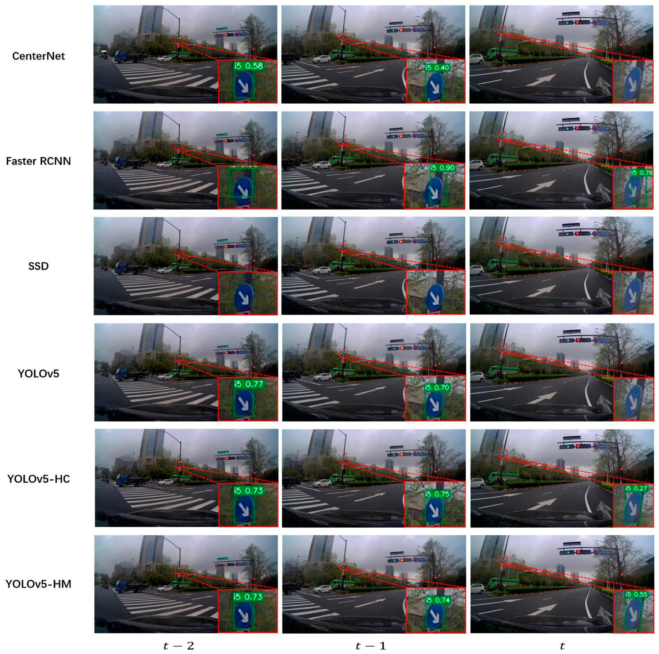
The on-board camera, as shown in
Figure 12, takes continuous photos of the same instance as the vehicle moves. Except for the SSD with poor overall performance, the remaining detectors achieved accurate detection and recognition in the first two frames. However, the majority of the detectors exhibited a missed detection at moment t due to deformation. Although the deformed traffic signs were detected by YOLOv5-HC, the result had a low confidence level. In contrast, because YOLOv5-HM utilizes detection information from multiple frames, the higher confidence in the first two frames is used in the sequence analysis to obtain a higher confidence at moment
.
To investigate the impact of MIM further, we ran
mAP calculations under various weather conditions and sample sizes, as shown in
Table 11. According to the results, YOLOv5-HM achieves an optimal value of 73.86 for the overall
mAP, an improvement of 1.07 over YOLOv5-HC. YOLOv5-HM outperforms the pre-improvement model in most sample size categories. YOLOv5-HM demonstrated the most substantial performance boost in sunny settings, with an overall
mAP improvement of 1.37. YOLOv5-HM, on the other hand, demonstrated a relatively smaller performance improvement in cloudy and rainy situations.
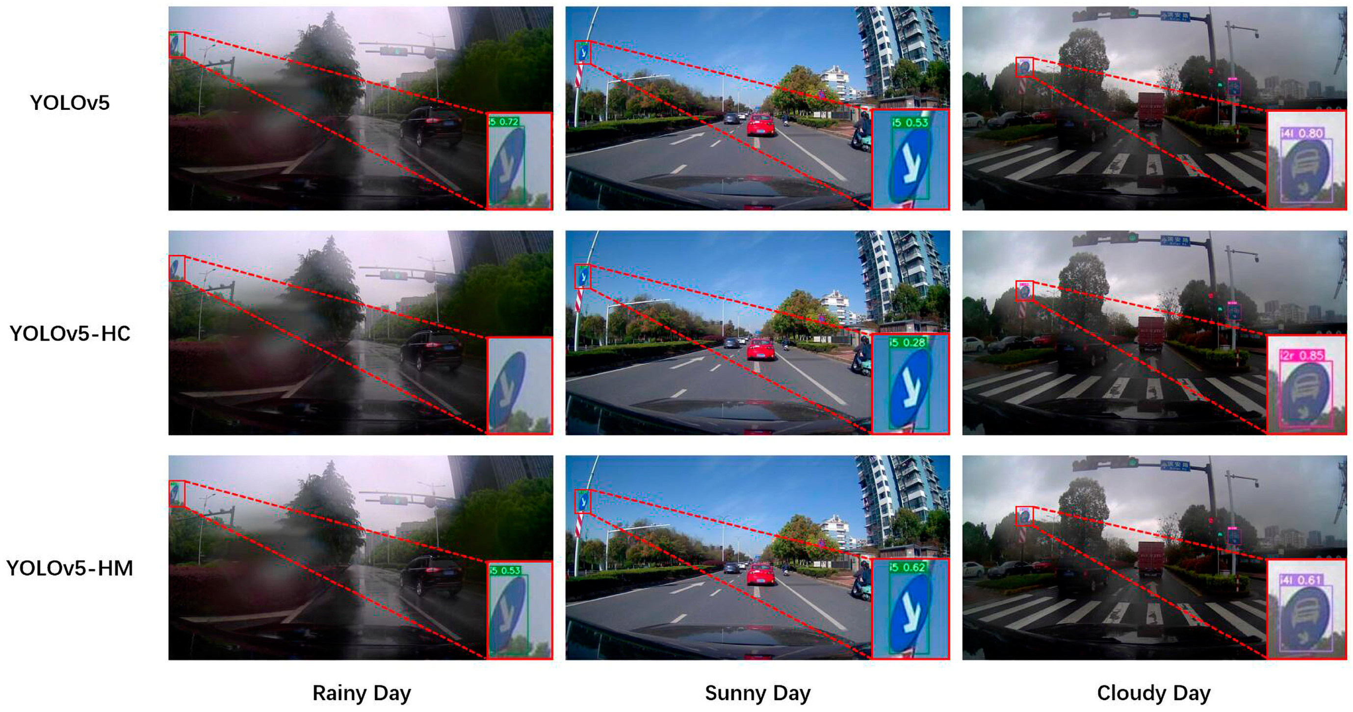
In order to indicate the impact of the improvements,
Figure 13 depicts examples of Yolov5 and the two upgraded models under various weather situations. In a rainy situation, YOLOv5-HC exhibits a missed detection due to deformation. After MIM processing, YOLOv5-HM achieves accurate detection and recognition, with a confidence of 0.53. A similar problem arises in sunny situations, where confidence is diminished due to deformation. In addition, the detector sometimes misclassifies. In the cloudy example, YOLOv5-HC misclassified the traffic sign as i2r. Since the classifications in the reference frames were all correct, YOLOv5-HM was able to correct this occasional misclassification using the detection information from multiple frames. In terms of inference speed, since MIM uses the feature embeddings extracted by the HCM, most of the increased computational effort comes from the calculation of the Euclidean distance in the association function, which hardly affects the inference time of the model.
4. Discussion
The evaluation results based on TT100K and ONCE demonstrate that the feature pyramid structure is critical in dealing with small objects and scale variations. At the same time, the test results reveal a shortcoming in the localization accuracy of the Faster RCNN, which originates from the coarseness of the feature map and the limited information offered by the candidate boxes [
48]. Furthermore, the evaluation findings on classes with varying sample sizes show that the long-tailed distribution has a considerable detrimental impact on the detector’s performance. For reasons of inference speed and detection performance, YOLOv5 becomes a better choice. The use of YOLOv5 as a single classification detector allows for more efficient localization of traffic signs due to their unique color and shape features. Detecting the most challenging case in
Figure 11 also demonstrates increased localization performance.
To cope with detector performance loss caused by unequal distribution, we propose a hierarchical classification model (HCM) that divides traffic signs into three superclasses and corresponding subclasses. This classification makes use of the distribution characteristics of traffic signs. Specifically, mandatory signs are mostly in the category with a large sample size, whereas warning signs are mostly in the category with a small sample size. While the overall sample distribution exhibits a significant long-tailed distribution, the difference in sample size between subclasses within a superclass is much smaller.
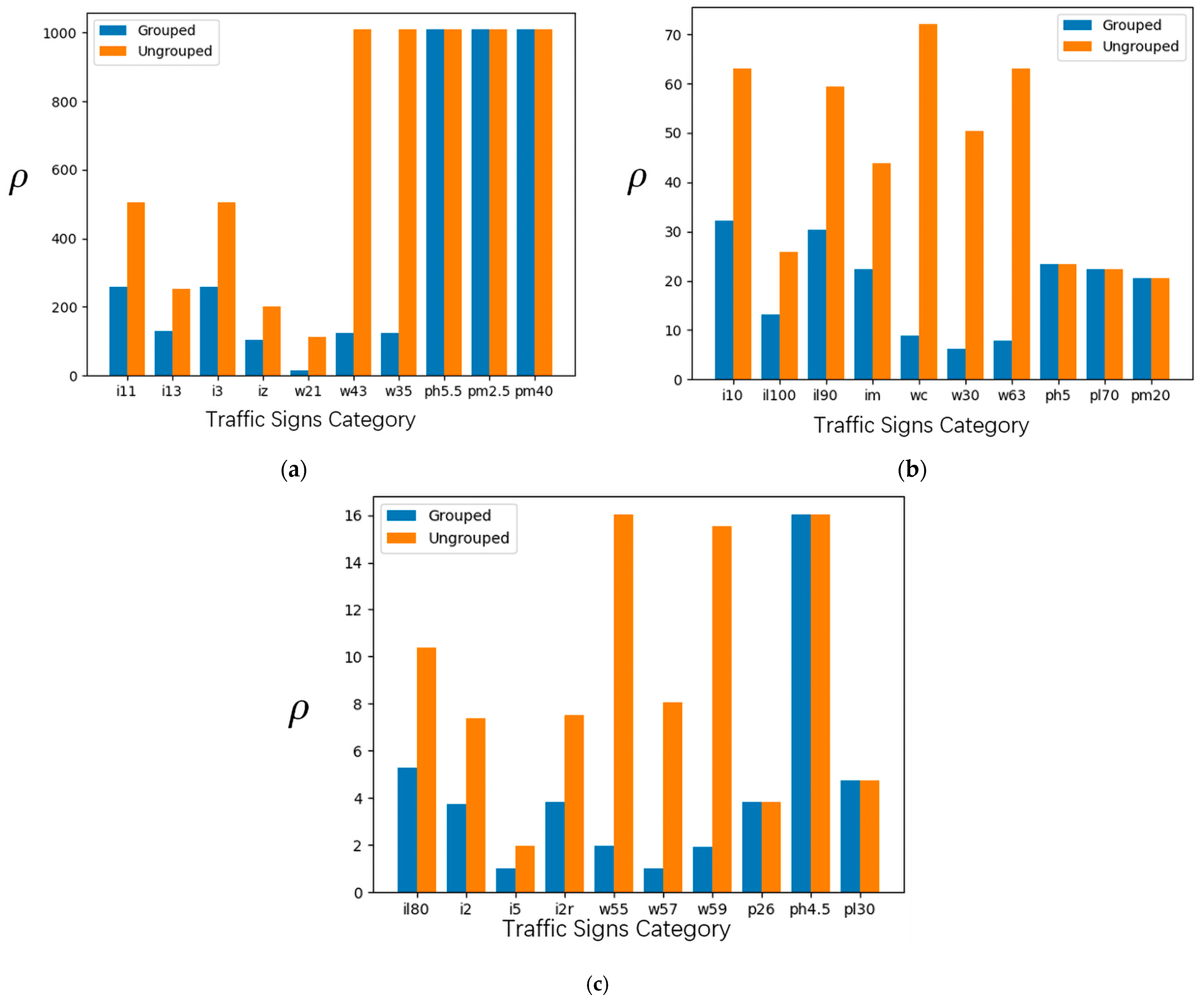
Equation (19) can be utilized to quantify the degree of imbalance in sample size between classes, which is calculated as the ratio of the maximum and minimum sample size across all categories [
42].
To clearly highlight the differences after grouping, some of the categories were randomly selected from the large, medium, and small categories.
Figure 14 indicates that after grouping, the sample distribution of traffic signs is more balanced, which is especially noticeable for warning traffic signs. Meanwhile, when the sample size falls, the reduction in
becomes bigger, resulting in more performance gains for YOLOv5-HC in the fewer sample categories. In addition, owing to its lightweight design, the HCM’s hierarchical classification structure does not considerably slow down inference speed. YOLOv5-HC is similar to the two-stage object detection algorithm, but the inference speed is much faster than Faster RCNN.
Small objects, scale variations, and long-tailed distributions are the main causes of detector performance degradation. Furthermore, real-world scenes contain anomalies such as deformation and occlusion, which frequently result in missed detections or misclassifications. Challenging cases generated by anomalies are difficult to solve since the anomalies result in missing or misleading image information. To overcome the limitations of a single image, our proposed multi-frame information integration module (MIM) integrates data from multiple detections to achieve robust detection and recognition. Meanwhile, correlation can be utilized to eliminate the redundant results produced by successive detections.
The evaluation results on the ONCE dataset demonstrate that MIM achieves a performance improvement in most cases. To further analyze the role of MIM, we varied the range of information integration by adjusting the number of reference frames. The data in
Table 12 show that as the number of reference frames increases, the performance of YOLOv5-HM gradually improves, indicating the significance of utilizing multi-frame information. However, since traffic signs in ONCE are typically photographed three times, there is no further improvement in model performance when the number of reference frames
in the experiment exceeds two.
5. Conclusions
In this paper, two novel and simple-to-implement modules are proposed to improve the performance of YOLOv5 for traffic sign detection and recognition. YOLOv5 provides outstanding localization performance for small objects and scale variations as a single classification detector. To reduce the negative impact of long-tailed distributions on classification, we propose a hierarchical classification module for the specific classification of traffic signs. Through grouping, HCM divides traffic signs into three superclasses and corresponding subclasses. The grouping takes advantage of traffic sign distributional characteristics, which can greatly reduce sample size discrepancies between classes. However, in the presence of anomalies such as occlusion and deformation, single-image-based algorithms still suffer from missing detection or misclassification. To deal with missing or misleading information caused by anomalies, this study designed a multi-frame information aggregation module to extract the detection sequence of traffic signs, which is based on the embedding generated by the HCM. The temporal sequence of detection information can deal with the shortcomings of a single image, reducing false detections caused by anomalies.
Experimental results based on TT100K show that YOLOv5-HC achieves a mAP of 79.0 in full classes, which exceeds state-of-the-art methods. At the same time, the inference speed of 22.7 FPS satisfies the real-time requirement. Furthermore, YOLOv5-HM using MIM outperformed YOLOv5-HC in terms of overall accuracy, with 0.67% improvement in precision, 1.32% improvement in recall, and 1.05 improvement in F1 score, respectively.
YOLOv5 has some shortcomings in traffic sign detection and consumes most of the computational resources. Therefore, we will improve the existing detection module in our research as more advanced object detection algorithms are proposed. Meanwhile, we will also try to improve the inference speed of the existing model using SNN, which can better balance the inference time and model accuracy. In addition, due to the uniqueness of the colors as well as the structure of the traffic signs, we also consider the use of VAE or statistical models to generate distributions that can be used for traffic sign recognition.
