

GNSS-Based Driver Assistance for Charging Electric City Buses: Implementation and Lessons Learned from Field Testing

Abstract
1. Introduction
- Our new approach to providing the ADAS system with precise vehicle pose estimates using only GNSS and internal bus sensors contributes to the area of GNSS for urban transport applications.
- A novel manoeuvre-planning algorithm that leverages affordable information sources (RTK GNSS, OpenStreetMap) and applies an optimisation technique to generate feasible trajectories under kinematic and geometric constraints in real time contributes to the area of motion planning for ADAS.
- As far as we know, this paper is the first to report the results of long-term extensive tests with a GNSS-based ADAS for buses in a real urban environment under regular daily traffic with passengers. Hence, it contributes to a better understanding of GNSS localisation as a means of supporting precise manoeuvres of city buses.
2. Related Work
3. Localisation of a City Bus with GNSS
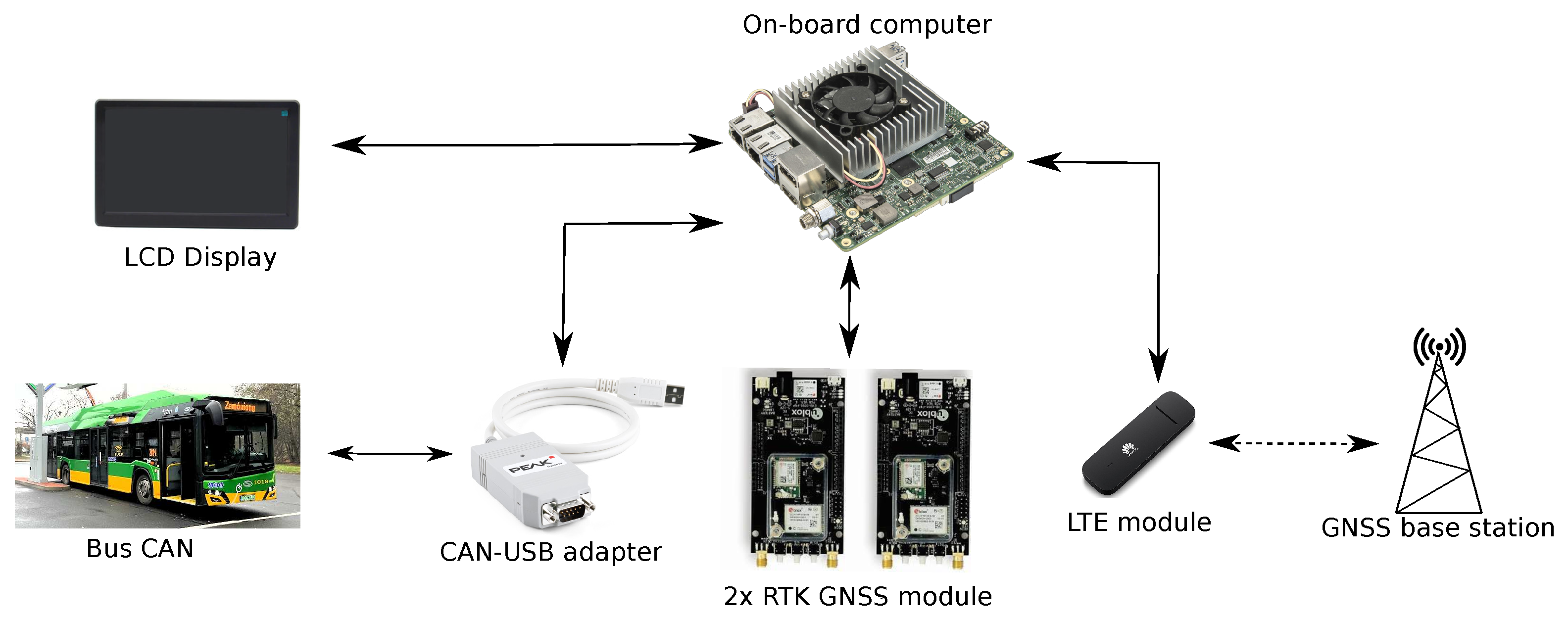
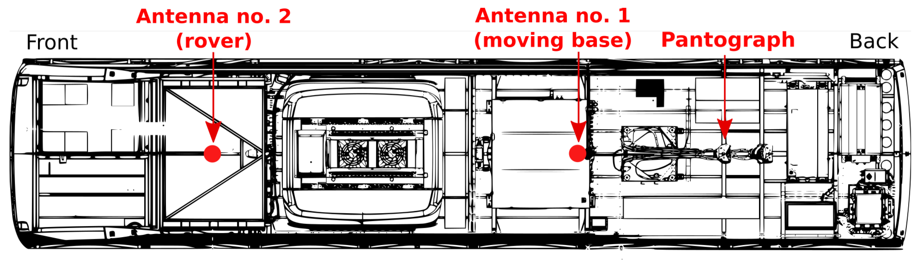
3.1. Hardware
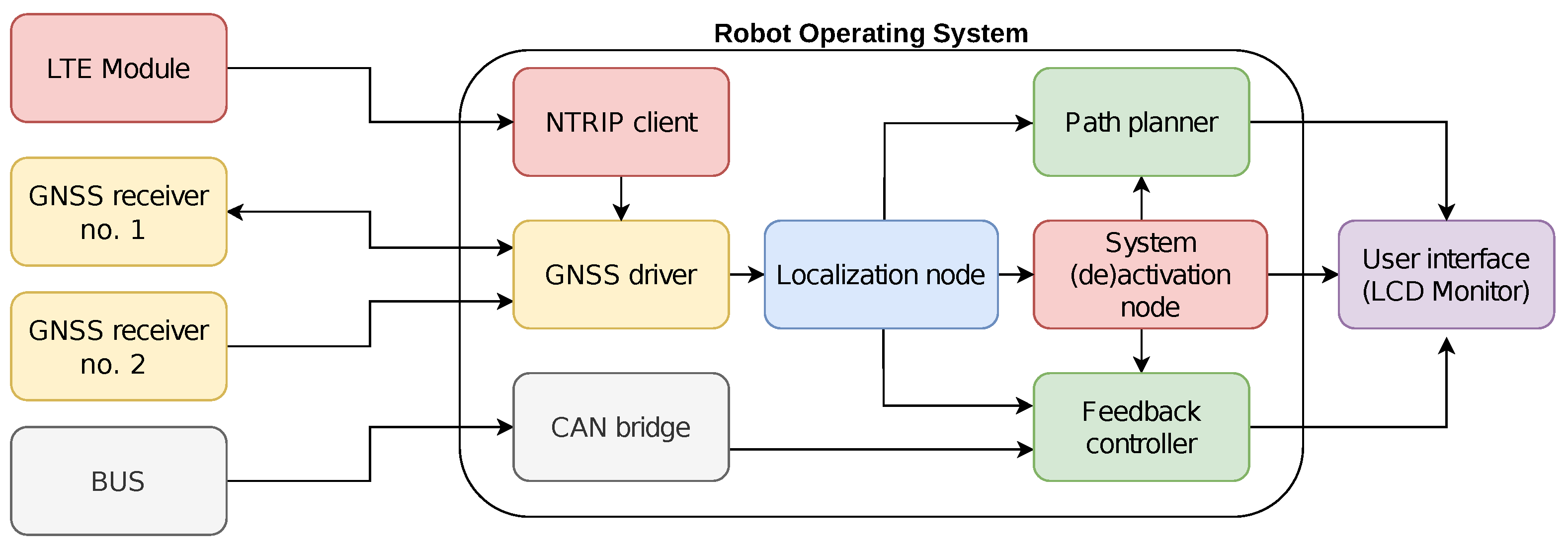
3.2. Software
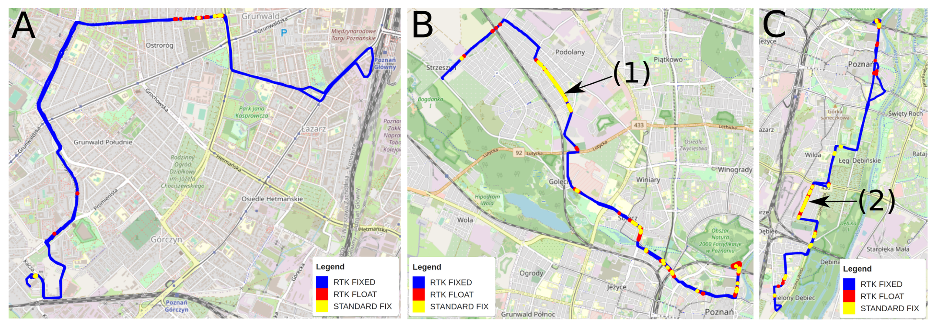
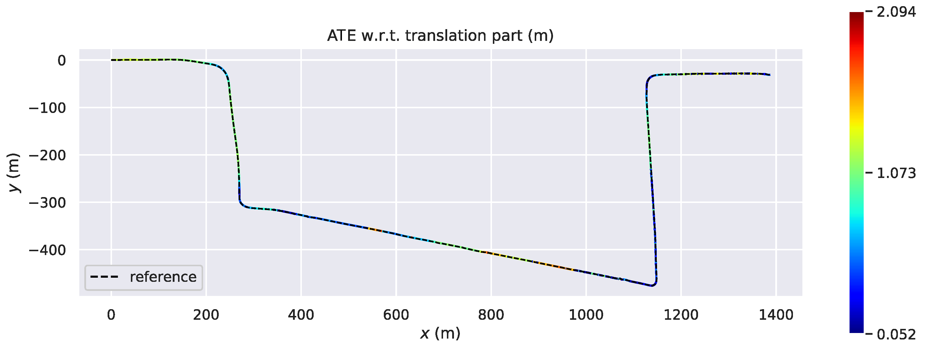
3.3. Performance Evaluation of the GNSS-Based Localisation System
4. Motion Planning and Control in ADAS for City Buses
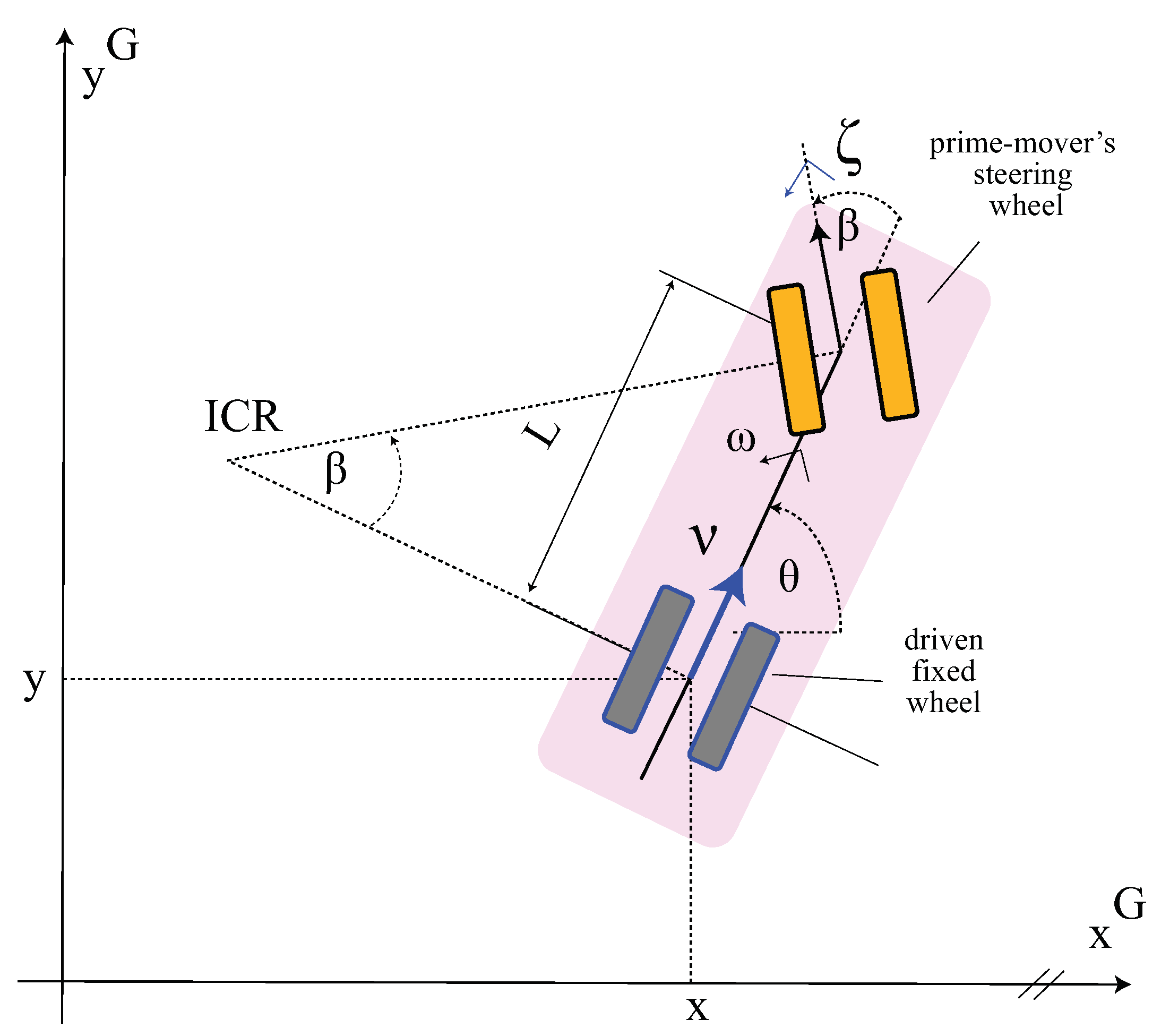
4.1. Bus Model for Low-Speed Manoeuvring
4.2. State Estimation
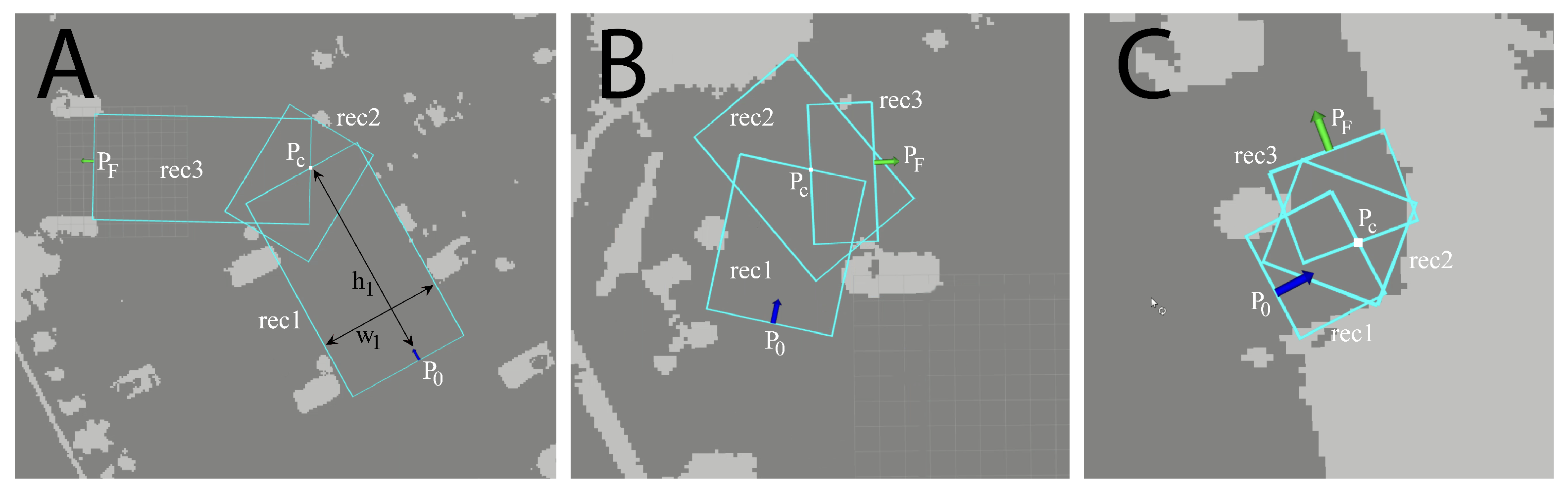
4.3. Path Planning in Restricted Areas
| Algorithm 1: Generating bounding rectangles. |
Input: initial and final configurations: and . functionCalculateWeight() while obstacle free do Expand the rectangle normal to the line segments h by . az end while return end function Calculate and lines along and . ▹ Calculate intersection point of two lines Output: The height h and weight w of each rectangles . |
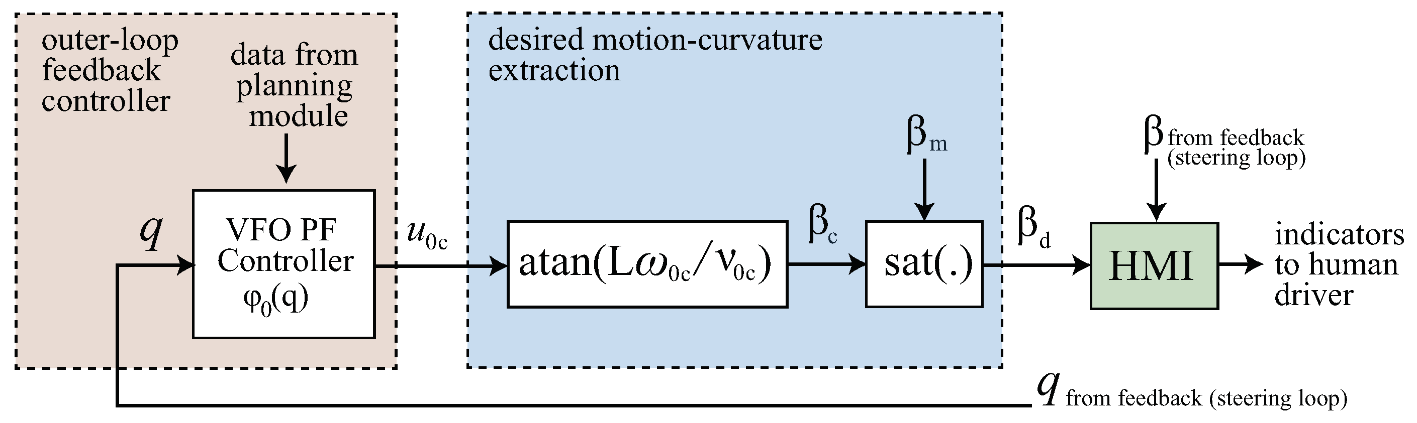
4.4. Feedback Control
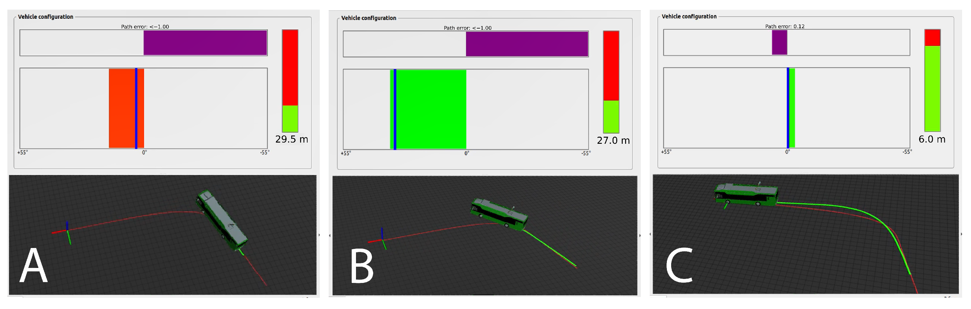
5. Human-Machine Interface in ADAS
6. Experimental Results
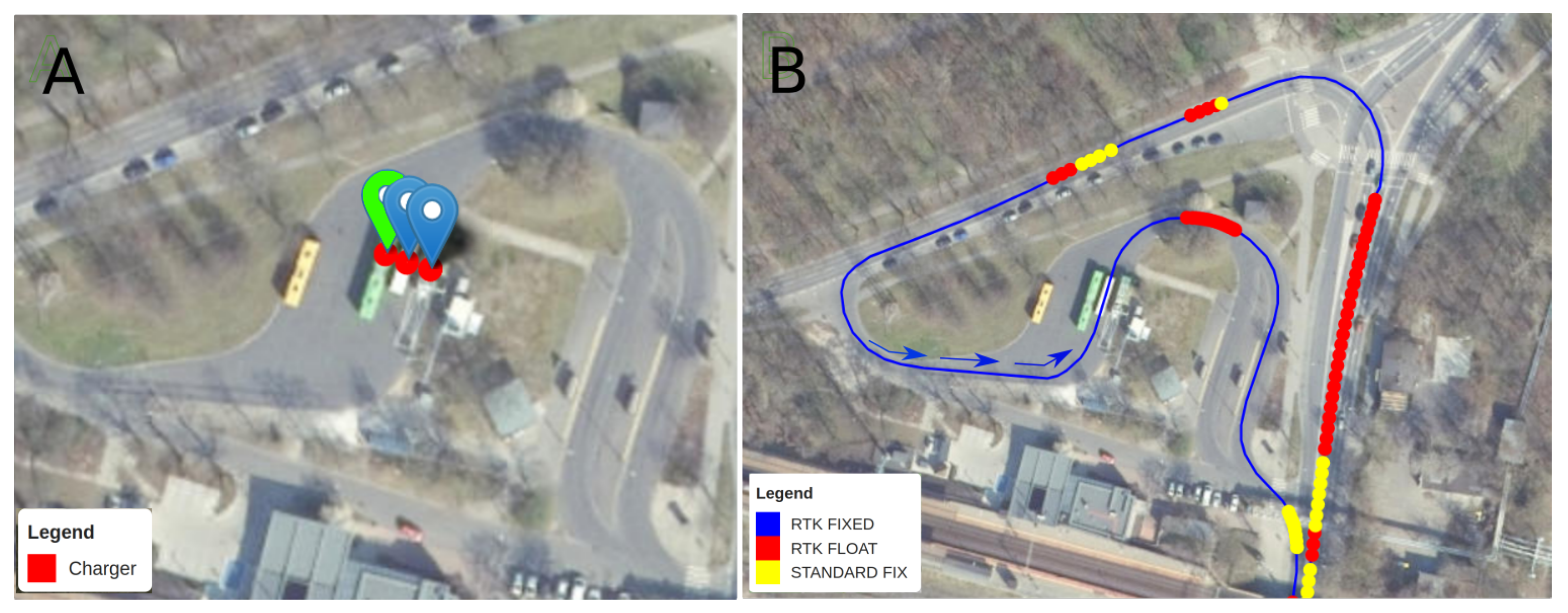
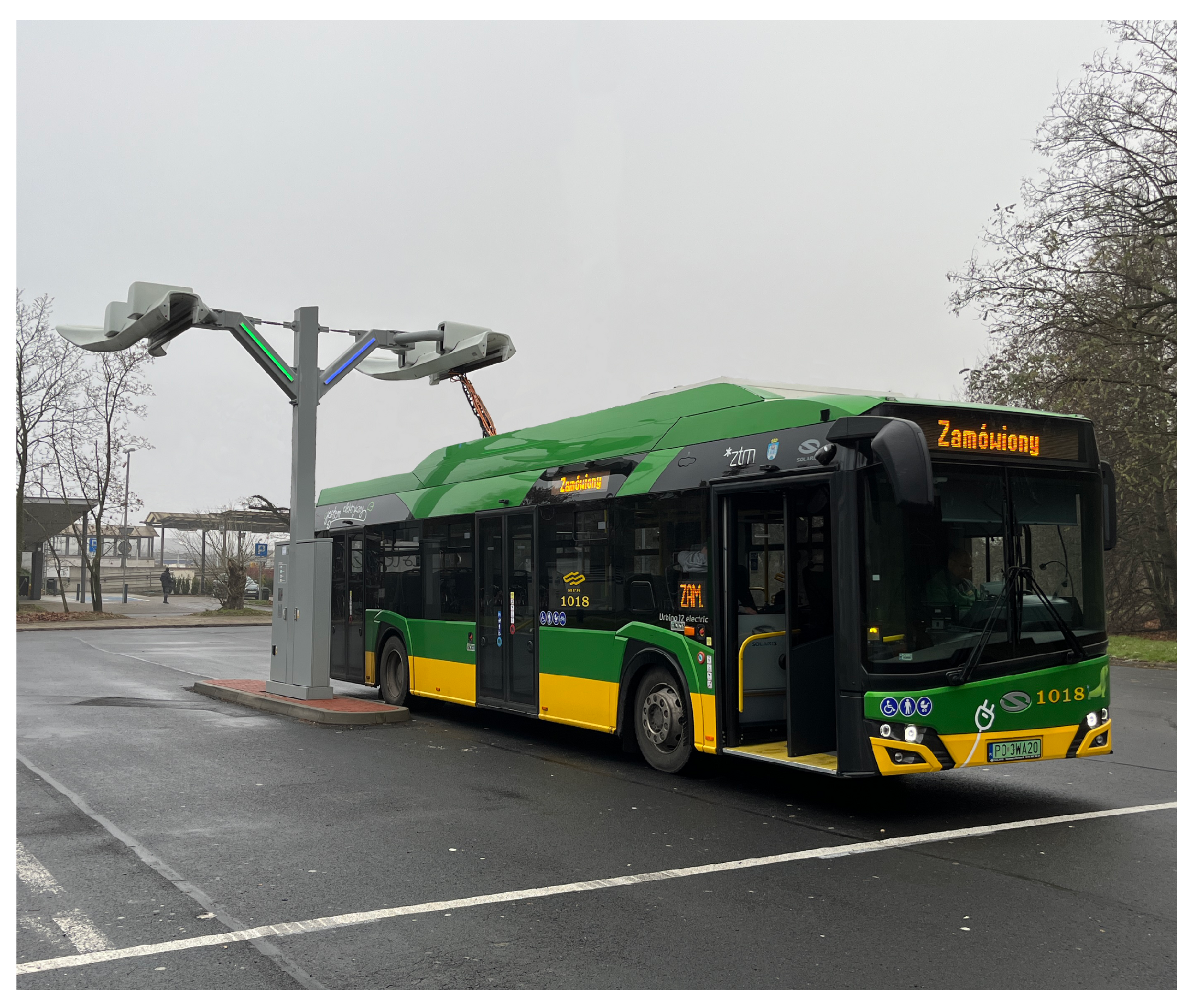
6.1. Environment and Scenario
6.2. Results of the Docking Experiments
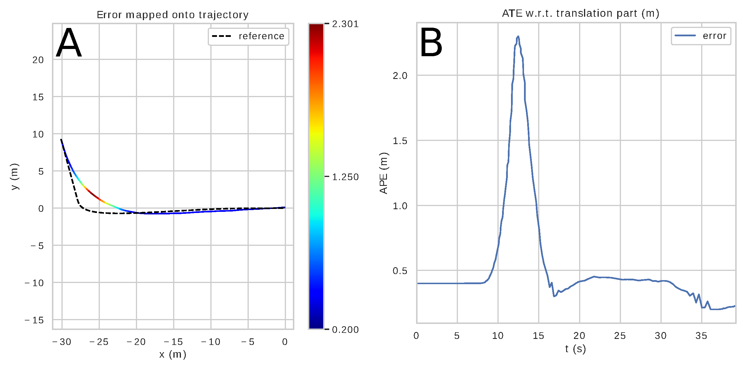
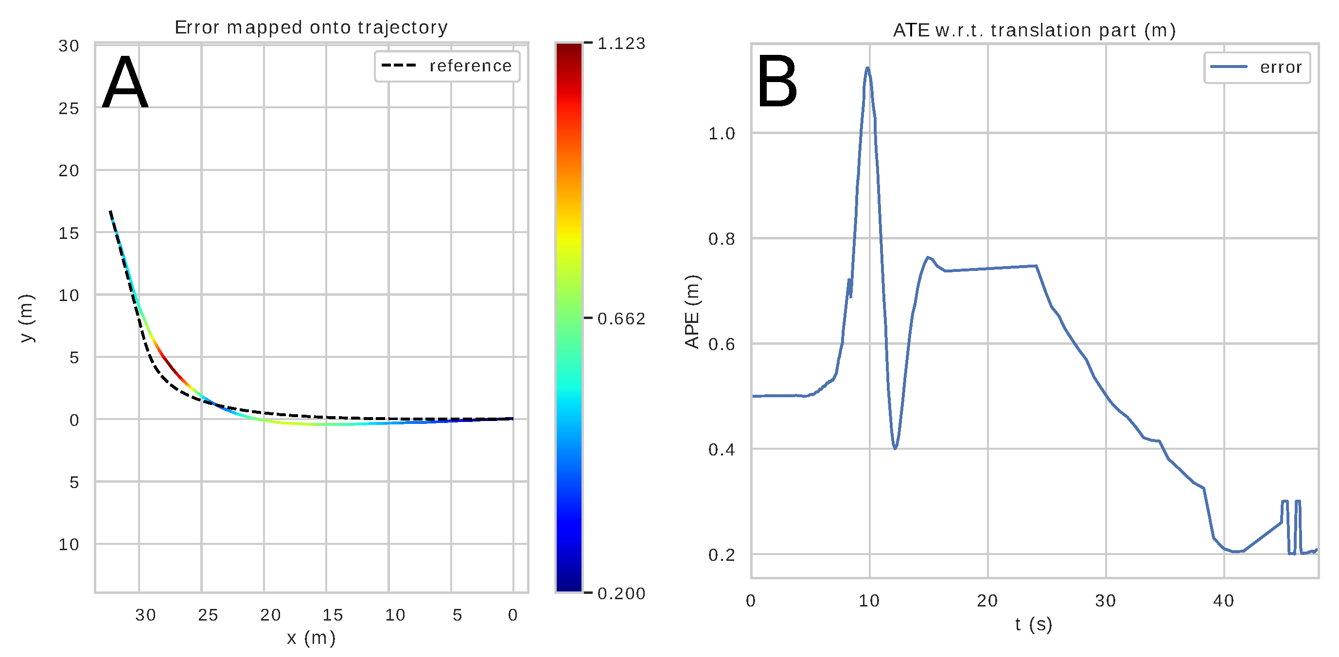
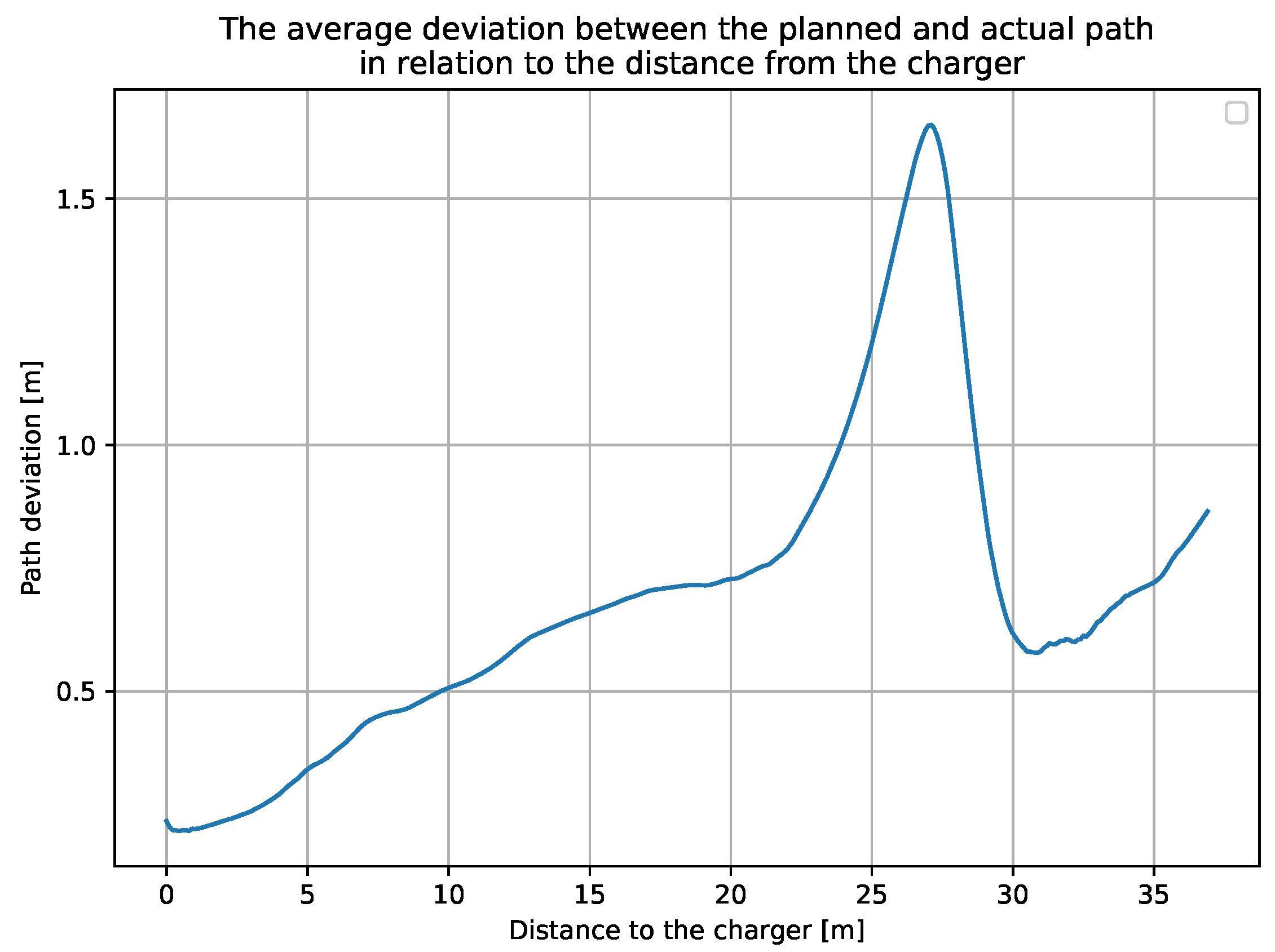
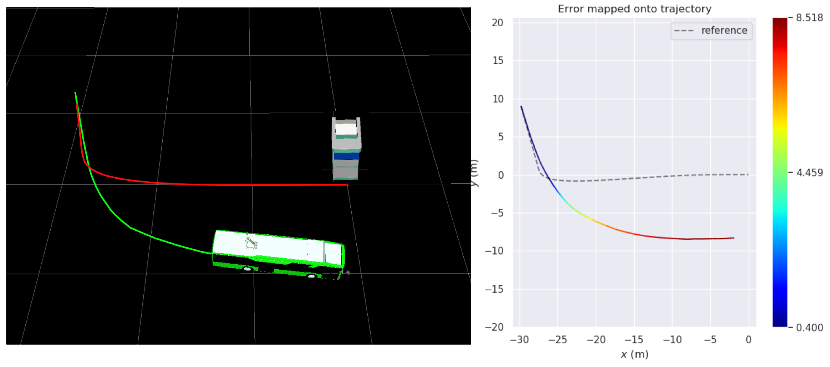
6.3. Accuracy of the Docking Manoeuvres
6.4. Failure Modes
7. Conclusions
Author Contributions
Funding
Data Availability Statement
Acknowledgments
Conflicts of Interest
References
- Vilppo, O.; Markkula, J. Feasibility of Electric Buses in Public Transport. World Electr. Veh. J. 2015, 7, 357–365. [Google Scholar] [CrossRef]
- Correa, G.; Muñoz, P.; Rodriguez, C. A comparative energy and environmental analysis of a diesel, hybrid, hydrogen and electric urban bus. Energy 2019, 187, 115906. [Google Scholar] [CrossRef]
- Michalek, M.M.; Gawron, T.; Nowicki, M.; Skrzypczynski, P. Precise Docking at Charging Stations for Large-Capacity Vehicles: An Advanced Driver-Assistance System for Drivers of Electric Urban Buses. IEEE Veh. Technol. Mag. 2021, 16, 57–65. [Google Scholar] [CrossRef]
- Shuttleworth, J. SAE Standards News: J3016 Automated-Driving Graphic Update. Available online: https://www.sae.org/news/2019/01/sae-updates-j3016-automated-driving-graphic (accessed on 4 April 2023).
- Nowak, T.; Nowicki, M.R.; Skrzypczyński, P. Vision-based positioning of electric buses for assisted docking to charging stations. Int. J. Appl. Math. Comput. Sci. 2022, 32, 583–599. [Google Scholar]
- Jiang, L.; Diao, X.; Zhang, Y.; Zhang, J.; Li, T. Review of the Charging Safety and Charging Safety Protection of Electric Vehicles. World Electr. Veh. J. 2021, 12, 184. [Google Scholar] [CrossRef]
- Deng, R.; Liu, Y.; Chen, W.; Liang, H. A Survey on Electric Buses: Energy Storage, Power Management, and Charging Scheduling. IEEE Trans. Intell. Transp. Syst. 2021, 22, 9–22. [Google Scholar] [CrossRef]
- Ma, T.Y.; Fang, Y. Survey of charging management and infrastructure planning for electrified demand-responsive transport systems: Methodologies and recent developments. Eur. Transp. Res. Rev. 2022, 14, 1866–8887. [Google Scholar] [CrossRef]
- Iclodean, C.; Cordos, N.; Varga, B.O. Autonomous Shuttle Bus for Public Transportation: A Review. Energies 2020, 13, 2917. [Google Scholar] [CrossRef]
- Bengler, K.; Dietmayer, K.; Farber, B.; Maurer, M.; Stiller, C.; Winner, H. Three Decades of Driver Assistance Systems: Review and Future Perspectives. IEEE Intell. Transp. Syst. Mag. 2014, 6, 6–22. [Google Scholar] [CrossRef]
- Ye, W.; Xu, Y.; Zhou, F.; Shi, X.; Ye, Z. Investigation of Bus Drivers’ Reaction to ADAS Warning System: Application of the Gaussian Mixed Model. Sustainability 2021, 13, 8759. [Google Scholar] [CrossRef]
- Chada, S.K.; Thomas, J.M.; Görges, D.; Ebert, A.; Teutsch, R. Ecological Adaptive Cruise Control for City Buses based on Hybrid Model Predictive Control using PnG and Traffic Light Information. In Proceedings of the IEEE Vehicle Power and Propulsion Conference (VPPC), Gijon, Spain, 25–28 October 2021; pp. 1–7. [Google Scholar]
- Yang, D.; Seo, S.W. Traffic Light Detection using Attention-Guided Continuous Conditional Random Fields. In Proceedings of the International Conference on Electronics, Information, and Communication (ICEIC), Jeju, Republic of Korea, 6–9 February 2022; pp. 1–3. [Google Scholar]
- Roszyk, K.; Nowicki, M.R.; Skrzypczyński, P. Adopting the YOLOv4 Architecture for Low-Latency Multispectral Pedestrian Detection in Autonomous Driving. Sensors 2022, 22, 1082. [Google Scholar] [CrossRef]
- Pérez, J.; Nashashibi, F.; Lefaudeux, B.; Resende, P.; Pollard, E. Autonomous Docking Based on Infrared System for Electric Vehicle Charging in Urban Areas. Sensors 2013, 13, 2645–2663. [Google Scholar] [CrossRef] [PubMed]
- Al-Saadi, M.; Mathes, M.; Käsgen, J.; Robert, K.; Mayrock, M.; Mierlo, J.V.; Berecibar, M. Optimization and Analysis of Electric Vehicle Operation with Fast-Charging Technologies. World Electr. Veh. J. 2022, 13, 20. [Google Scholar] [CrossRef]
- Petrov, P.; Boussard, C.; Ammoun, S.; Nashashibi, F. A hybrid control for automatic docking of electric vehicles for recharging. In Proceedings of the IEEE International Conference on Robotics and Automation, Saint Paul, MN, USA, 14–18 May 2012; pp. 2966–2971. [Google Scholar]
- Miseikis, J.; Ruther, M.; Walzel, B.; Hirz, M.; Brunner, H. 3D Vision Guided Robotic Charging Station for Electric and Plug-in Hybrid Vehicles. arXiv 2017, arXiv:1703.05381. [Google Scholar]
- Gu, Y.; Hsu, L.T.; Kamijo, S. Towards lane-level traffic monitoring in urban environment using precise probe vehicle data derived from three-dimensional map aided differential GNSS. IATSS Res. 2018, 42, 248–258. [Google Scholar] [CrossRef]
- Lee, W.; Cho, H.; Hyeong, S.; Chung, W. Practical Modeling of GNSS for Autonomous Vehicles in Urban Environments. Sensors 2019, 19, 4236. [Google Scholar] [CrossRef] [PubMed]
- Viandier, N.; Marais, J.; De Verdalle, E.; Prestail, A. Positioning urban buses: GNSS performances. In Proceedings of the 8th International Conference on ITS Telecommunications, Phuket, Thailand, 24–24 October 2008; pp. 51–55. [Google Scholar] [CrossRef]
- Yang, Y.; Yan, J.; Guo, J.; Kuang, Y.; Yin, M.; Wang, S.; Ma, C. Driving Behavior Analysis of City Buses Based on Real-Time GNSS Traces and Road Information. Sensors 2021, 21, 687. [Google Scholar] [CrossRef]
- Swaminathan, H.B.; Sommer, A.; Becker, A.; Atzmueller, M. Performance Evaluation of GNSS Position Augmentation Methods for Autonomous Vehicles in Urban Environments. Sensors 2022, 22, 8419. [Google Scholar] [CrossRef]
- Kuutti, S.; Fallah, S.; Katsaros, K.; Dianati, M.; Mccullough, F.; Mouzakitis, A. A Survey of the State-of-the-Art Localization Techniques and Their Potentials for Autonomous Vehicle Applications. IEEE Internet Things J. 2018, 5, 829–846. [Google Scholar] [CrossRef]
- Zhu, N.; Marais, J.; Bétaille, D.; Berbineau, M. GNSS Position Integrity in Urban Environments: A Review of Literature. IEEE Trans. Intell. Transp. Syst. 2018, 19, 2762–2778. [Google Scholar] [CrossRef]
- Marais, J.; Meurie, C.; Attia, D.; Ruichek, Y.; Flancquart, A. Toward accurate localization in guided transport: Combining GNSS data and imaging information. Transp. Res. Part C Emerg. Technol. 2014, 43, 188–197. [Google Scholar] [CrossRef]
- Viandier, N.; Nahimana, D.F.; Marais, J.; Duflos, E. GNSS Performance Enhancement in Urban Environment Based on Pseudo-Range Error Model. In Proceedings of the Location and Navigation Symposium (PLANS), Monterey, CA, USA, 5–8 May 2008; pp. 377–382. [Google Scholar] [CrossRef]
- Joerger, M.; Pervan, B. Autonomous Ground Vehicle Navigation Using Integrated GPS and Laser-scanner Measurements. In Proceedings of the IEEE/ION Position, Location, and Navigation Symposium, San Diego, CA, USA, 25–27 April 2006; pp. 988–997. [Google Scholar]
- Wen, W.; Pfeifer, T.; Bai, X.; Hsu, L.T. It is time for Factor Graph Optimization for GNSS/INS Integration: Comparison between FGO and EKF. arXiv 2020, arXiv:2004.10572. [Google Scholar]
- Liu, J.; Gao, W.; Hu, Z. Optimization-Based Visual-Inertial SLAM Tightly Coupled with Raw GNSS Measurements. In Proceedings of the IEEE International Conference on Robotics and Automation (ICRA), Xi’an, China, 30 May–5 June 2021; pp. 11612–11618. [Google Scholar]
- Ćwian, K.; Nowicki, M.R.; Skrzypczyński, P. GNSS-Augmented LiDAR SLAM for Accurate Vehicle Localization in Large Scale Urban Environments. In Proceedings of the 17th International Conference on Control, Automation, Robotics and Vision (ICARCV), Singapore, 11–13 December 2022; pp. 701–708. [Google Scholar] [CrossRef]
- Ng, K.M.; Johari, J.; Abdullah, S.A.C.; Ahmad, A.; Laja, B.N. Performance Evaluation of the RTK-GNSS Navigating under Different Landscape. In Proceedings of the 18th International Conference on Control, Automation and Systems (ICCAS), Pyeongchang, Republic of Korea, 17–20 October 2018; pp. 1424–1428. [Google Scholar]
- Michałek, M.; Kiełczewski, M. The concept of passive control assistance for docking maneuvers with n-trailer vehicles. IEEE/ASME Trans. Mechatron. 2015, 20, 2075–2084. [Google Scholar] [CrossRef]
- Gawron, T.; Mydlarz, M.; Michalek, M.M. Algorithmization of constrained monotonic maneuvers for an advanced driver assistant system in the intelligent urban buses. In Proceedings of the IEEE Intelligent Vehicles Symposium, Paris, France, 9–12 June 2019; pp. 232–238. [Google Scholar]
- Michałek, M.M.; Patkowski, B.; Gawron, T. Modular Kinematic Modelling of Articulated Buses. IEEE Trans. Veh. Technol. 2020, 69, 8381–8394. [Google Scholar] [CrossRef]
- Michałek, M.; Gawron, T. VFO Path following Control with Guarantees of Positionally Constrained Transients for Unicycle-Like Robots with Constrained Control Input. J. Intell. Robot. Syst. 2018, 89, 191–210. [Google Scholar] [CrossRef]
- Gawron, T.; Michałek, M.M. VFO Path Following Control Strategy for Constrained Motion of Car-Like Robots with Invariant Funnels Computed Using the SOS Optimization. In Proceedings of the 2018 IEEE Conference on Control Technology and Applications (CCTA), Copenhagen, Denmark, 21–24 August 2018; pp. 94–100. [Google Scholar]
- Gao, L.; Xiong, L.; Xia, X.; Lu, Y.; Yu, Z.; Khajepour, A. Improved Vehicle Localization Using On-Board Sensors and Vehicle Lateral Velocity. IEEE Sens. J. 2022, 22, 6818–6831. [Google Scholar] [CrossRef]
- Liu, W.; Xia, X.; Xiong, L.; Lu, Y.; Gao, L.; Yu, Z. Automated Vehicle Sideslip Angle Estimation Considering Signal Measurement Characteristic. IEEE Sens. J. 2021, 21, 21675–21687. [Google Scholar] [CrossRef]
- Xia, X.; Hashemi, E.; Xiong, L.; Khajepour, A. Autonomous Vehicle Kinematics and Dynamics Synthesis for Sideslip Angle Estimation Based on Consensus Kalman Filter. IEEE Trans. Control. Syst. Technol. 2023, 31, 179–192. [Google Scholar] [CrossRef]
- Lee, H.G.; Kang, D.H.; Kim, D.H. Human–Machine Interaction in Driving Assistant Systems for Semi-Autonomous Driving Vehicles. Electronics 2021, 10, 2405. [Google Scholar] [CrossRef]
- Biondi, F.N.; Getty, D.; McCarty, M.M.; Goethe, R.M.; Cooper, J.M.; Strayer, D.L. The Challenge of Advanced Driver Assistance Systems Assessment: A Scale for the Assessment of the Human–Machine Interface of Advanced Driver Assistance Technology. Transp. Res. Rec. 2018, 2672, 113–122. [Google Scholar] [CrossRef]
- Lilis, Y.; Zidianakis, E.; Partarakis, N.; Ntoa, S.; Stephanidis, C. A Framework for Personalised HMI Interaction in ADAS Systems. In Proceedings of the 5th International Conference on Vehicle Technology and Intelligent Transport Systems—Volume 1: VEHITS, Heraklion, Crete, Greece, 3–5 May 2019; pp. 586–593. [Google Scholar] [CrossRef]
- Masola, A.; Gabbi, C.; Castellano, A.; Capodieci, N.; Burgio, P. Graphic Interfaces in ADAS: From Requirements to Implementation. In Proceedings of the 6th EAI International Conference on Smart Objects and Technologies for Social Good, Antwerp, Belgium, 14–16 September 2020; pp. 193–198. [Google Scholar] [CrossRef]
- Bedkowski, J.; Nowak, H.; Kubiak, B.; Studzinski, W.; Janeczek, M.; Karas, S.; Kopaczewski, A.; Makosiej, P.; Koszuk, J.; Pec, M.; et al. A Novel Approach to Global Positioning System Accuracy Assessment, Verified on LiDAR Alignment of One Million Kilometers at a Continent Scale, as a Foundation for Autonomous DRIVING Safety Analysis. Sensors 2021, 21, 5691. [Google Scholar] [CrossRef]
- Janos, D.; Kuras, P.; Ortyl, L. Evaluation of low-cost RTK GNSS receiver in motion under demanding conditions. Measurement 2022, 201, 111647. [Google Scholar] [CrossRef]
- u-Blox. ZED-F9P, u-Blox F9P High Precision GNSS Module. 2023. Available online: https://content.u-blox.com/sites/default/files/documents/ZED-F9P-01B_DataSheet_UBX-17051259.pdf (accessed on 12 April 2023).
- Ho, V.; Rauf, K.; Passchier, I.; Rijks, F.; Witsenboer, T. Accuracy Assessment of RTK GNSS based Positioning Systems for Automated Driving. In Proceedings of the 15th Workshop on Positioning, Navigation and Communications (WPNC), Bremen, German, 25–26 October 2018; pp. 1–6. [Google Scholar]
- Nowicki, M.R. A data-driven and application-aware approach to sensory system calibration in an autonomous vehicle. Measurement 2022, 194, 111002. [Google Scholar] [CrossRef]
- Rietdorf, A.; Daub, C.; Loef, P. Precise positioning in real-time using navigation satellites and telecommunication. In Proceedings of the 3rd Workshop on Positioning, Navigation and Communication (WPNC), Hannover, Germany, 16 March 2006; pp. 209–218. [Google Scholar]
- Michałek, M.; Kozłowski, K. Feedback control framework for car-like robots using the unicycle controllers. Robotica 2012, 30, 517–535. [Google Scholar] [CrossRef]
- Pivtoraiko, M.; Knepper, R.A.; Kelly, A. Differentially Constrained Mobile Robot Motion Planning in State Lattices. J. Field Robot. 2009, 26, 308–333. [Google Scholar] [CrossRef]
- Andersson, J.A.E.; Gillis, J.; Horn, G.; Rawlings, J.B.; Diehl, M. CasADi—A software framework for nonlinear optimization and optimal control. Math. Program. Comput. 2019, 11, 1–36. [Google Scholar] [CrossRef]
- Wächter, A.; Biegler, L. On the Implementation of an Interior-Point Filter Line-Search Algorithm for Large-Scale Nonlinear Programming. Math. Program. 2006, 106, 25–57. [Google Scholar] [CrossRef]
- EC Engineering. Current Collection System for Charging of Electric Buses 2023. Available online: https://ec-e.pl/wp-content/uploads/2022/01/ec_eng_A3_v7_EN_1.pdf (accessed on 12 April 2023).


| Sequence (Bus Stops) | Distance | Time | Num. of Precision RTK FIXED Poses | Num. of Poses in Low Precision Modes |
|---|---|---|---|---|
| Dworzec Zachodni–Kacza | 7.483 km | 34.77 min | 20,558 | 284 |
| Garbary PKM–Strzeszyn | 11.616 km | 42.42 min | 23,749 | 1691 |
| Garbary PKM–Os. Dębina | 9.290 km | 43.93 min | 25,264 | 1090 |
| Sequence (Bus Stops) | ||||
|---|---|---|---|---|
| Dworzec Zachodni–Kacza | 0.276 m | 3.113 m | 0.175 m | 0.213 m |
| Garbary PKM–Strzeszyn | 0.602 m | 4.377 m | 0.428 m | 0.423 m |
| Garbary PKM–Os. Dębina | 0.619 m | 4.340 m | 0.440 m | 0.436 m |
| Sequence (Bus Stops) | ||||
|---|---|---|---|---|
| part of Garbary PKM–Os. Dębina | 0.777 m | 2.0943 m | 0.640 m | 0.439 m |
| Seq. | ||||
|---|---|---|---|---|
| 1 | 0.680 m | 1.585 m | 0.558 m | 0.390 m |
| 2 | 0.423 m | 0.668 m | 0.391 m | 0.159 m |
| 3 | 0.649 m | 1.600 m | 0.527 m | 0.379 m |
| 4 | 1.370 m | 3.193 m | 0.985 m | 0.953 m |
| 5 | 0.866 m | 2.247 m | 0.626 m | 0.599 m |
| 6 | 0.765 m | 1.966 m | 0.575 m | 0.504 m |
| 7 | 0.766 m | 1.967 m | 0.599 m | 0.479 m |
| 8 | 1.270 m | 3.141 m | 0.872 m | 0.923 m |
| 9 | 0.535 m | 1.084 m | 0.471 m | 0.254 m |
| 10 | 1.001 m | 2.562 m | 0.716 m | 0.700 m |
| 11 | 0.910 m | 2.294 m | 0.679 m | 0.605 m |
| 12 | 0.808 m | 2.068 m | 0.618 m | 0.520 m |
| 13 | 0.688 m | 1.745 m | 0.536 m | 0.432 m |
| 14 | 0.892 m | 2.282 m | 0.662 m | 0.597 m |
| 15 | 0.543 m | 1.347 m | 0.478 m | 0.258 m |
| 16 | 1.501 m | 3.584 m | 1.028 m | 1.093 m |
| 17 | 0.574 m | 1.152 m | 0.503 m | 0.277 m |
| 18 | 0.875 m | 2.257 m | 0.638 m | 0.599 m |
| 19 | 0.626 m | 1.295 m | 0.543 m | 0.311 m |
| 20 | 0.923 m | 2.281 m | 0.708 m | 0.592 m |
| 21 | 0.525 m | 1.211 m | 0.473 m | 0.229 m |
| 22 | 0.547 m | 1.267 m | 0.479 m | 0.265 m |
| 23 | 0.644 m | 2.166 m | 0.535 m | 0.358 m |
| 24 | 0.746 m | 1.820 m | 0.593 m | 0.452 m |
| 25 | 0.529 m | 1.075 m | 0.473 m | 0.237 m |
| 26 | 0.944 m | 2.423 m | 0.684 m | 0.651 m |
| 27 | 0.561 m | 1.238 m | 0.510 m | 0.234 m |
| 28 | 0.560 m | 1.354 m | 0.472 m | 0.303 m |
| 29 | 0.889 m | 2.301 m | 0.649 m | 0.606 m |
| 30 | 0.600 m | 1.317 m | 0.517 m | 0.306 m |
| 31 | 1.135 m | 2.863 m | 0.790 m | 0.815 m |
| 32 | 0.506 m | 1.009 m | 0.449 m | 0.234 m |
| 33 | 0.612 m | 1.500 m | 0.504 m | 0.347 m |
| 34 | 0.858 m | 2.224 m | 0.646 m | 0.565 m |
| 35 | 0.987 m | 2.506 m | 0.721 m | 0.675 m |
| 36 | 0.725 m | 1.861 m | 0.567 m | 0.453 m |
| 37 | 0.895 m | 3.138 m | 0.671 m | 0.593 m |
| 38 | 1.192 m | 4.372 m | 0.781 m | 0.901 m |
| 39 | 0.897 m | 3.093 m | 0.655 m | 0.613 m |
| 40 | 0.623 m | 1.560 m | 0.504 m | 0.368 m |
| 41 | 0.556 m | 1.319 m | 0.476 m | 0.287 m |
| 42 | 0.577 m | 1.381 m | 0.491 m | 0.303 m |
| 43 | 0.537 m | 1.123 m | 0.479 m | 0.241 m |
| 44 | 0.603 m | 1.342 m | 0.520 m | 0.304 m |
| 45 | 1.140 m | 2.861 m | 0.859 m | 0.749 m |
| 46 | 1.420 m | 3.466 m | 0.960 m | 1.047 m |
| 47 | 1.169 m | 2.896 m | 0.811 m | 0.842 m |
| 48 | 1.570 m | 5.257 m | 1.014 m | 1.199 m |
| 49 | 1.000 m | 2.560 m | 0.708 m | 0.707 m |
| 50 | 0.587 m | 1.299 m | 0.506 m | 0.297 m |
| Seq. | ||
|---|---|---|
| 1 | 0.039 m | 0.053 m |
| 2 | −0.009 m | −0.028 m |
| 3 | −0.373 m | 0.178 m |
| 4 | 0.043 m | 0.042 m |
| 5 | −0.403 m | −0.042 m |
| 6 | 0.369 m | 0.028 m |
| 7 | 0.262 m | 0.095 m |
| 8 | 0.154 m | 0.161 m |
| 9 | −0.099 m | −0.053 m |
| 10 | −0.146 m | −0.035 m |
| 11 | 0.476 m | 0.060 m |
| 12 | −0.013 m | 0.031 m |
| 13 | 0.116 m | −0.038 m |
| 14 | 0.390 m | −0.024 m |
| 15 | 0.026 m | −0.063 m |
| 16 | 0.150 m | −0.073 m |
| 17 | 0.412 m | 0.021 m |
| 18 | −0.223 m | −0.091 m |
| 19 | 0.189 m | 0.077 m |
| 20 | 0.051 m | −0.028 m |
| 21 | 0.167 m | −0.017 m |
| 22 | 0.120 m | 0.000 m |
| 23 | 0.021 m | −0.003 m |
| 24 | 0.180 m | 0.000 m |
| 25 | 0.056 m | −0.087 m |
| 26 | 0.356 m | 0.011 m |
| 27 | 0.335 m | 0.014 m |
| 28 | −0.051 m | −0.119 m |
| 29 | 0.176 m | −0.038 m |
| 30 | 0.429 m | 0.028 m |
| 31 | −0.051 m | −0.119 m |
| 32 | 0.013 m | −0.080 m |
| 33 | 0.086 m | −0.112 m |
| 34 | 0.167 m | 0.179 m |
| 35 | −0.335 m | −0.063 m |
| 36 | −0.124 m | −0.039 m |
| 37 | 0.064 m | −0.059 m |
| 38 | −0.013 m | 0.031 m |
| 39 | 0.163 m | 0.042 m |
| 40 | 0.322 m | 0.046 m |
| 41 | 0.077 m | −0.091 m |
| 42 | 0.017 m | −0.042 m |
| 43 | 0.468 m | 0.081 m |
| 44 | −0.189 m | 0.070 m |
| 45 | 0.017 m | 0.007 m |
| 46 | −0.210 m | −0.025 m |
| 47 | −0.322 m | 0.052 m |
| 48 | −0.236 m | −0.060 m |
| 49 | −0.004 m | −0.185 m |
| 50 | 0.056 m | 0.109 m |
| 0.063 m | 0.219 m | −0.004 m | 0.077 m |
Disclaimer/Publisher’s Note: The statements, opinions and data contained in all publications are solely those of the individual author(s) and contributor(s) and not of MDPI and/or the editor(s). MDPI and/or the editor(s) disclaim responsibility for any injury to people or property resulting from any ideas, methods, instructions or products referred to in the content. |
© 2023 by the authors. Licensee MDPI, Basel, Switzerland. This article is an open access article distributed under the terms and conditions of the Creative Commons Attribution (CC BY) license (https://creativecommons.org/licenses/by/4.0/).
Share and Cite
Esfandiyar, I.; Ćwian, K.; Nowicki, M.R.; Skrzypczyński, P. GNSS-Based Driver Assistance for Charging Electric City Buses: Implementation and Lessons Learned from Field Testing. Remote Sens. 2023, 15, 2938. https://doi.org/10.3390/rs15112938
Esfandiyar I, Ćwian K, Nowicki MR, Skrzypczyński P. GNSS-Based Driver Assistance for Charging Electric City Buses: Implementation and Lessons Learned from Field Testing. Remote Sensing. 2023; 15(11):2938. https://doi.org/10.3390/rs15112938
Chicago/Turabian StyleEsfandiyar, Iman, Krzysztof Ćwian, Michał R. Nowicki, and Piotr Skrzypczyński. 2023. "GNSS-Based Driver Assistance for Charging Electric City Buses: Implementation and Lessons Learned from Field Testing" Remote Sensing 15, no. 11: 2938. https://doi.org/10.3390/rs15112938
APA StyleEsfandiyar, I., Ćwian, K., Nowicki, M. R., & Skrzypczyński, P. (2023). GNSS-Based Driver Assistance for Charging Electric City Buses: Implementation and Lessons Learned from Field Testing. Remote Sensing, 15(11), 2938. https://doi.org/10.3390/rs15112938