Review

Ground-Penetrating Radar and Electromagnetic Induction: Challenges and Opportunities in Agriculture

by
Sashini Pathirana
1,
Sébastien Lambot
2,
Manokarajah Krishnapillai
1,
Mumtaz Cheema
1,
Christina Smeaton
1 and
Lakshman Galagedara
1,*
1
School of Science and the Environment, Memorial University of Newfoundland, Corner Brook, NL A2H 5G4, Canada
2
Earth and Life Institute, Université Catholique de Louvain, 1348 Louvain-la-Neuve, Belgium
*
Author to whom correspondence should be addressed.
Remote Sens. 2023, 15(11), 2932; https://doi.org/10.3390/rs15112932
Submission received: 17 April 2023 / Revised: 24 May 2023 / Accepted: 1 June 2023 / Published: 4 June 2023
(This article belongs to the Section Environmental Remote Sensing)

Abstract

:
Information on the spatiotemporal variability of soil properties and states within the agricultural landscape is vital to identify management zones supporting precision agriculture (PA). Ground-penetrating radar (GPR) and electromagnetic induction (EMI) techniques have been applied to assess soil properties, states, processes, and their spatiotemporal variability. This paper reviews the fundamental operating principles of GPR and EMI, their applications in soil studies, advantages and disadvantages, and knowledge gaps leading to the identification of the difficulties in integrating these two techniques to complement each other in soil data studies. Compared to the traditional methods, GPR and EMI have advantages, such as the ability to take non-destructive repeated measurements, high resolution, being labor-saving, and having more extensive spatial coverage with geo-referenced data within agricultural landscapes. GPR has been widely used to estimate soil water content (SWC) and water dynamics, while EMI has broader applications such as estimating SWC, soil salinity, bulk density, etc. Additionally, GPR can map soil horizons, the groundwater table, and other anomalies. The prospects of GPR and EMI applications in soil studies need to focus on the potential integration of GPR and EMI to overcome the intrinsic limitations of each technique and enhance their applications to support PA. Future advancements in PA can be strengthened by estimating many soil properties, states, and hydrological processes simultaneously to delineate management zones and calculate optimal inputs in the agricultural landscape.

Graphical Abstract

1. Introduction

An increasing global population, coupled with the uncertainty of climate change, is resulting in an agricultural expansion to improve food security. This expansion is highlighting the need for the application of innovative technologies to increase and optimize food productivity. Consequently, agricultural expansion (i.e., the conversion of natural lands into agriculture) and the associated increased agrochemical inputs have resulted in adverse environmental impacts such as the pollution of land and water resources, thereby impacting the food chain and subsequently affecting the health of the soil, water, people, flora, and fauna [1,2,3,4]. The excessive use of agrochemicals increases the accumulation of harmful chemicals in the soil, groundwater, and water bodies [5]. Minimizing the environmental and socio-economic threats caused by the expansion and intensification of agriculture may be conducted by implementing precise agricultural strategies [1,6,7].
Precision agriculture (PA), supported by various technologies, is a rapidly emerging field for managing the agricultural landscape on a large scale by considering the field variability for increasing agricultural productivity while minimizing negative environmental impacts and the production cost [6,8,9]. Agricultural practices such as irrigation, land preparation, and fertilization are typically applied uniformly across the entire field, treating the heterogeneous fields as homogeneous. However, the spatial and temporal heterogeneity of the agricultural landscape can be effectively monitored through implementing different technologies to support PA, including (1) geographic information systems (GIS), (2) satellite-based global positioning systems (GPS), (3) remote sensing, (4) drones, (5) the Internet of Things, (6) artificial intelligence, and (7) different proximal sensors, for example, geophysical techniques [2,6,10]. These digital technologies are applied to collect, process, monitor, and map the spatiotemporal variability of the agricultural landscape. Their purpose is to improve agronomic performance, enhance crop productivity and develop decision support tools [4,6,9,11,12,13,14,15,16,17]. By utilizing the latest technologies, such as unmanned aerial vehicles, agricultural machinery, and robotic technologies, the required amounts of water, nutrients, and agrochemicals for plant growth and development can be accurately applied to specific locations within the agricultural landscape and within the appropriate timeframe [1,2,4,6,12,13,18,19]. PA offers several benefits, including improved soil fertility and health, increased water productivity and food security, minimized soil and water pollution, and reduced labor force requirements, as well as the overuse of resources such as water, fertilizer, seeds, and energy, leading to lower production costs [1,2,3,4,20]. The incorporation of spatiotemporal variability mapping with geo-statistics and GIS marked a major advance in PA to a new level to identify management zones [11,12,21].
The spatiotemporal variability of crop factors and subsurface physical, chemical, and hydrological properties, and processes are crucial in PA [6]. Hydro-geophysics is an efficient approach that includes multi-scale probing and high-resolution imaging techniques for accurately obtaining the spatiotemporal variability of the subsurface hydrological processes and soil properties [22,23,24,25]. Traditional methods such as soil sampling and laboratory analysis are destructive, labor-intensive, costly in large scales, time-consuming, and mainly provide point scale measurements only [6,22,26,27]. Commonly used geophysical techniques in hydro-geophysics are electrical resistivity tomography, electromagnetic induction (EMI), self-potential, ground-penetrating radar (GPR), induced polarization, surface nuclear magnetic resonance, gravity, magnetics, and seismic methods [25,26,27,28]. However, not all these techniques are commonly used in PA applications. The main limitations of these geophysical techniques are their complexity of use, poor automation ability, and high initial capital cost. In addition, they mainly provide indirect proxy information only; thus, some instruments, such as EMI, need site-specific calibration [17,25,29,30]. Among these geophysical techniques, this article mainly reviews applications of GPR and EMI as rapidly emerging electromagnetic techniques in soil studies to estimate the spatiotemporal variation of soil properties with particular emphasis on agricultural applications. GPR and EMI applications have some advantages in the agricultural landscape compared to the other geophysical methods. For example, the electrical resistivity method requires electrode installation. Therefore, it disturbs the subsurface and is time-consuming for large-scale applications. On the other hand, the sampling depth of the electrical resistivity and seismic methods is extensive and beyond the root zone.
The use of GPR and EMI has been extensively studied and documented in various fields, including forestry, archaeology, engineering, geology/geoengineering, and environmental science [29,31,32]. Moreover, GPR and EMI use in agriculture is also well documented with a focus on elucidating soil properties and states such as bulk density, porosity, soil compaction, soil texture, cation exchange capacity (CEC), soil salinity, clay content, soil organic matter (SOM), soil water content (SWC), infiltration capacity, and water holding capacity [28,29,32].
Huisman et al. [33] reviewed the estimation of SWC using various methods with GPR, including the reflected wave velocity, ground wave velocity, transmitted wave velocity (in boreholes), and surface reflection coefficient, while van Dam [34] discussed different calibration functions to estimate SWC using GPR. Liu et al. [35] and Klotzsche et al. [36] updated the review of Huisman et al. [33] by including modern techniques applied to estimate SWC, such as full-waveform inversion, average envelope amplitude, and the frequency shift method. Recently, Zajícová and Chuman [32] reviewed applications of GPR in soil studies, including SWC, stratigraphy, soil salinity, and soil texture, and Zhang et al. [37] reviewed GPR applications with SWC and soil hydraulic properties. Doolittle and Brevik [29] reviewed applications of EMI in soil studies, including soil properties such as soil salinity, SWC, soil texture, clay content, and CEC.
The majority of previous reviews have focused on either GPR or EMI with a singular focus on estimating SWC. This review builds upon yet differs from the above-mentioned reviews by summarizing a wide range of applications previously conducted to determine soil properties and states using GPR, EMI, or both. Additional properties discussed in this review include soil salinity, bulk density, soil porosity, and soil hydraulic properties. This review aims to provide a comprehensive overview of the use of GPR and EMI techniques in soil studies for estimating critical agricultural soil information.
This article reviewed >250 peer-reviewed journal articles, conference papers, and books primarily related to the principles and applications of GPR and EMI in agriculture and soil studies (Figure 1). Metadata analysis was conducted using keywords associated with GPR and EMI applications in soil studies. GPR and EMI applications are graphically presented and summarized as percentage data (Figure 1). Co-occurrence term maps were developed for the past 15 years (2007–2022) by referring to the number of articles on GPR and EMI applications in agriculture based on keywords to focus on the latest research articles to support future directions (Figure 1).
This review begins with the general background information and discusses electromagnetic methods, including their theoretical and empirical background. The review then discusses GPR and its fundamental principles, as well as their application to soil studies, including SWC, porosity, compaction, soil salinity, hydraulic properties, groundwater table, and capillary fringe reflection. Then, this review discusses EMI and its basic principles, along with its applications to soil studies, including soil salinity, SWC, bulk density, soil compaction, and some applications with magnetic susceptibility. Finally, the review offers insights, synthesis, and critical analysis, while the summary and future directions section presents an overview and highlights areas for future research.

2. Electromagnetic Methods

Maxwell’s equations mathematically describe the physics of electromagnetic (EM) waves and related medium properties. Constitutive equations quantify three physical properties of materials, namely, (1) electrical conductivity (σ), (2) permittivity (ε), and (3) magnetic permeability (µ), concerning the electromagnetic field [38,39,40].
GPR and EMI are the most used near-surface geophysical techniques/proximal sensors in agriculture and related fields that use electromagnetic waves [17,28]. The advantages of these two techniques include the ability to survey a relatively large area within a short time and with the minimal land disturbance, thereby allowing for repeated measurements at the exact location, with a larger sample volume compared with the traditional methods and relatively low operational costs [29,41]. GPR uses high-frequency (VHF-UHF) electromagnetic waves, while EMI uses relatively low-frequency (VLF) electromagnetic waves in various applications. Low-frequency and high-frequency fields have different sensitivities with respect to their material properties, different operational methods, and applications in soil studies (Table 1).

2.1. Theoretical and Empirical Equations and Models Used in Applications of Electromagnetic Methods

2.1.1. Topp’s Equation

Topp et al. [42] developed an empirical relationship, i.e., a third-degree polynomial equation,
θ v = 5.3   ×   10 2 + 2.92   ×   10 2 ε r 5.5   ×   10 4 ε r 2 + 4.3   ×   10 6 ε r 3
between the soil’s relative dielectric permittivity εr and volumetric water content (θv).
This relationship was assessed against the effect of soil texture, bulk density, temperature, soluble salts, and hysteresis and found to be relatively independent of these properties [42]. Topp’s equation is the most widely applied and accepted empirical equation in GPR applications since it is simple, relatively accurate, and valid for fully and partially saturated conditions [43]. However, in peat or organic-rich and heavy clay soils, the applicability of this relationship has limitations [44,45,46].

2.1.2. Archie’s Equation

Archie [47] developed two empirical relationships between the apparent electrical conductivity (σa), soil water saturation (SW), pore water electrical conductivity (σw), and porosity (φ) of porous rocks by conducting laboratory experiments. In this relationship, n is the saturation exponent and m is the cementation exponent. Archie’s first equation was developed for the resistivity of fully saturated porous rocks, and the second law was developed for partly saturated porous rocks [47]. Shah and Singh [48], Ewing and Hunt [49], and Glover [50,51] modified Archie’s equation,
σ a = 1 a φ m S w n σ w
and applied it to soils.

2.1.3. Complex Refractive Index Model

The complex refractive index model (CRIM) is a three-phase (solid—s, water—w, and air—a) volumetric mixing model. The CRIM equation is a theoretical approach that describes the bulk εr as a function of φ and SW [52]:
Ԑ r ( b ) α = φ S W ε r ( w ) α + 1 φ ε r s α + φ ( 1   S w ) ε r ( a ) α
The geometric factor (α) is related to the orientation of the electric field concerning the geometry of the solid phase. In GPR applications, CRIM estimates properties such as SW and φ with acceptable accuracy [53,54,55].

2.1.4. Rhoades’s Equation

Rhoades et al. [56] developed a relationship between σa as a function of SWC (θ) and σw:
σa = σw θT + σs
where T is the transmission coefficient considering the tortuosity of the flow path as water content changes. The bulk surface electrical conductivity (σs) is connected with the mobile ions at the soil–liquid interface.

3. Ground-Penetrating Radar

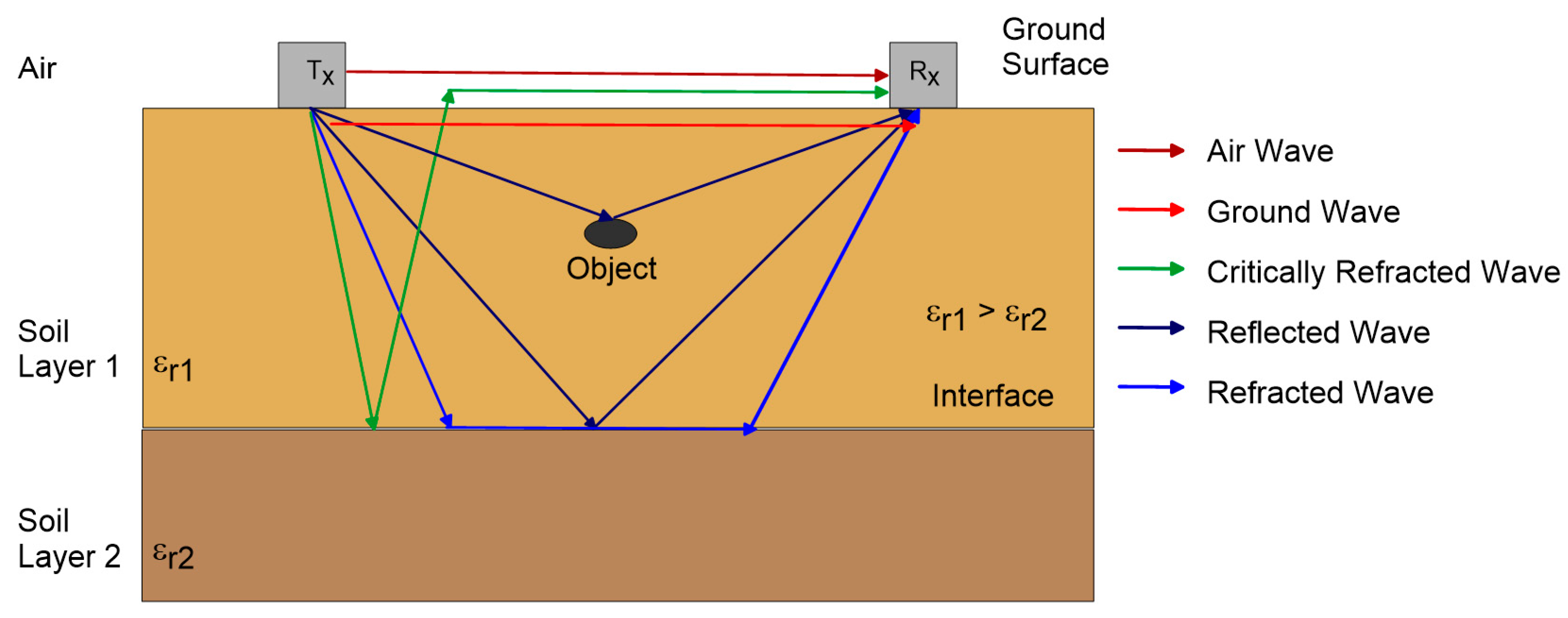
3.1. Basic Operating Principles of Ground-Penetrating Radar

GPR is a near-surface electromagnetic proximal sensor commonly used in agriculture and environmental applications [57,58,59]. Commercially available GPR systems use unguided electromagnetic waves with frequencies ranging from 10 MHz to 3600 MHz [36,58]. Resolution and depth of penetration are vital factors of GPR applications. Radar wave propagation velocity and wave attenuation depend on primary electromagnetic properties such as the relative dielectric permittivity (εr), electric conductivity σ, and magnetic permeability (µ) of the soil/media [58,59]. εr is mainly controlled by the water content of the subsurface as the permittivity of liquid water overwhelms those of other soil constituents [42,58]. Equation (5)
v = c ε r
shows the relationship between velocity (v) and εr, where c is the propagation velocity of electromagnetic waves in free space, which is equal to the speed of light (0.3 m/ns) [58]. The penetration depth of GPR is mainly determined by the σ of subsurface materials and the operation frequency [33,41,57,58]. When EM waves travel through conductive materials, EM energy is lost as heat through the electrical current. In addition, energy loss in EM waves is due to increasing operating frequency and scattering. This energy loss is called attenuation and, therefore, reduces the penetration depth of GPR waves [57,58,60,61]. GPR wave attenuation also results from geometrical spreading in 3D wave propagation. The resolution of GPR increases with increasing frequency, increasing bandwidth, and decreasing wave velocity, since the wavelength (λ) is inversely proportional to the frequency (f) and directly proportional to the velocity (λ = v/f) [61,62,63]. The radiation pattern of a GPR antenna is the primary determinant of its footprint, which is the subsurface area illuminated by the radiation emitted from the antenna. The shape and extent of the radiation pattern depend on several factors, including the antenna design, frequency, size, shape, and dielectric properties of the subsurface. The beam width of the radiation pattern is also affected by the dielectric permittivity of the subsurface, with higher permittivity resulting in a narrower beam.
The most common GPR system consists of an impulse generator that repeatedly sends a source of a particular voltage and frequency to a transmitting antenna. It is worth noting that frequency-domain radars are also available in addition to impulse radars and are also referred to as time-domain radars [64]. They operate by successively transmitting continuous waves over a specific frequency range. Ground-coupled and air-coupled horn antennas are used for on-ground and air-borne GPR surveys, respectively (Figure 2).
A commonly used GPR system consists of two antennas: a transmitter (Tx) and a receiver (Rx) or multiple receivers. The TX generates electromagnetic waves, following the frequency-dependent antenna radiation pattern, which travels through the air, air-surface interface, and subsurface. As shown in Figure 3, the Rx receives airwave, direct ground wave (DGW), reflected wave, and refracted waves [57,58,65]. EM wave reflection or refraction at a boundary depends on different electrical properties (mainly εr in most GPR applications) of the layer above and below the boundary [66].
GPR applications have three main data acquisition modes: (1) reflection profiling, (2) velocity-sounding, and (3) transillumination [57,58,61]. In the reflection profiling method, the Tx and Rx antennas are kept in a fixed antenna separation, orientation, and station interval, and both antennas are moved along the survey direction [57]. This method is called the common offset method or fixed offset method (FOM) and produces a vertical 2D image of the subsurface reflections (Figure 4a) [61,67]. The GPR velocity-sounding method can be performed using the common mid-point (CMP) method or the wide-angle reflection and refraction (WARR) method. In the CMP method, Tx and Rx are moved apart from each other by keeping the midpoint between the two antennas fixed (Figure 4b). However, in the WARR method, one antenna (Tx, for example) is kept at a fixed location, and the other antenna (Rx) is moved away by increasing the antenna offset (Figure 4c). The objectives of the velocity-sounding methods are to estimate the velocity by measuring the two-way travel times for different antenna offsets and then finding the slope of the relationship between the squared travel time and antenna offset [57,61]. The transillumination survey method places the Tx and Rx on opposite sides of the medium. Under transillumination, zero-offset profiling (ZOP) is a quick method to find anomalous zones by moving Tx and Rx from one station to another at a predetermined step size (Figure 4d). In the multi-offset gathering (MOG) mode, one antenna (Tx) is kept stationary while the other antenna (Rx) is moved to multiple locations to produce tomographic imaging (Figure 4e). In vertical reflection profiling (VRP), Tx is placed on the surface, and Rx is placed in the borehole since this method has many advantages over ZOP and MOG (Figure 4f). The data acquisition method and frequency selected in each survey are based on the application requirements and field conditions [57,58,68,69].

3.2. Applications of Ground-Penetrating Radar in Soil Studies

This section discusses the applications of GPR to estimate soil properties; states such as SWC, porosity, compaction, salinity, texture, SOM, and other applications such as depth to the groundwater table and capillarity.

3.2.1. Soil Water Content

SWC estimation is the most extensively used and well-developed GPR application in soil studies. The large-scale estimation and mapping of the spatiotemporal variability of SWC are critical across the agricultural landscape, but these are difficult tasks to complete with traditional methods. For example, mapping high resolution SWC variability using GPR provides the information necessary to optimize the amount of water required for and the timing of crop irrigation. According to previous studies, volumetric soil water content (SWCV) can be estimated from GPR using various methods such as the reflected wave velocity method, DGW velocity method, transmitted wave velocity method (in boreholes), surface reflection coefficient method, average envelope amplitude (AEA) method, and full-waveform inversion (FWI) method. Subsurface SWC influences the propagation velocity of GPR waves since εr varies with SWC and velocity varies with εr [40,61]. The well-established and widely used Topp’s equation [42] estimates SWCV from εr. Capacitance probes, neutron probes, the gravimetric method, and time domain reflectometry (TDR) are used for validating GPR-estimated SWC [67,69,70,71,72,73,74,75,76].
  • Reflected wave velocity method
The reflected wave velocity method is used to acquire SWCV in deeper soil layers. However, reflectors such as isolated objects or interfaces are required to obtain the travel time of the reflected radar wave. Natural reflectors such as rocks and roots and artificial reflectors such as pipes are point reflectors, while lithologic layers and the water table are interfaces [41,71,72,77,78,79]. The two-way travel time of the GPR wave above the reflector is measured and converted into radar wave velocity, then to εr, and is then used to calculate the SWCV [76,80,81]. The velocity of the reflected wave is obtained using an FOM or multiple offset methods (MOM): CMP or WARR. When the depth of the reflector is known, the reflected wave velocity is estimated in the FOM by dividing the depth of the reflector by the two-way travel time. Lunt et al. [80] applied the reflected wave velocity method under natural conditions, while Stoffregen et al. [82], Loeffler and Bano [83], Ercoli et al. [81], and Zhou et al. [84] applied it under controlled conditions to obtain SWCV. With advanced analysis techniques, the average velocity of a reflector can be obtained by fitting a hyperbola [76,85,86,87]. On the other hand, CMP and WARR methods are applied as multiple offset methods when the depth of the reflector is unknown. However, data collection and processing in this method are time-consuming and labor-intensive [35,36]. Steelman and Endress [88] applied the multi-frequency CMP method in three different sites to estimate the vertical variation of SWCV with the reflected wave method during a complete annual cycle, including wetting/drying and freezing/thawing. The reflection method for determining SWCV has some limitations, as it depends on the continuous availability of reflectors, especially in shallow soils [76].
b.
Direct ground wave velocity method
On the other hand, the DGW velocity method of GPR can be used to estimate the SWCV of shallow (uppermost centimeters) soils without employing a reflector [35,67,71,74,89]. Both the FOM and MOM can be used to estimate SWCV from the direct ground wave, though the MOM is time-consuming and laborious compared to the FOM [67,89]. To address this, Sperl [63] established a method to estimate SWCV over a large area by combining the MOM and FOM. In this method, the MOM only decides the most suitable antenna separation to distinguish between the DGW and the direct airwave. Then, the FOM is applied with the decided antenna separation to collect data effectively over a large area [35,90]. Huisman et al. [89] assessed the accuracy of DGW to estimate and map SWCV over a large area with WARR and the FOM (single trace analysis). The accuracy of SWC estimated based on WARR measurements was ±0.030 m3/m3, while it was ±0.037 m3/m3 based on the FOM when compared with the TDR method. Therefore, the authors suggested that the available TDR calibrations, such as Topp’s equation [42], can also be applied to GPR [89]. Furthermore, the authors suggested that the most appropriate assessment between electromagnetic methods (TDR and GPR) is εr, rather than SWCV. Galagedara et al. [67] and Huisman and Bouten [73] discussed the importance of accurate time-zero calibration to estimate SWCV using the DGW method. Huisman and Bouten [73] conducted a sensitivity analysis to study time-zero error at zero antennae offset with WARR measurements. The authors found that GPR simulations could not account for the meantime shift at zero offset due to the time-picking error and SWCV heterogeneity in the sensitivity analysis. Galagedara et al. [67] suggested an accurate and stable time-zero picking methodology to estimate SWCV with an error rate of less than 1% under variable water contents.
Huisman et al. [91] found that GPR is an efficient technique to map SWCV over an agricultural landscape, and GPR-estimated water content matched well with TDR results. The accuracy and spatial and temporal variability of the SWC under different water contents, such as irrigation and drainage conditions, have been studied by several researchers [67,72,74,77,91,92,93,94]. In addition, SWC variation under dry and rainy seasons was studied by Thitimakorn et al. [95], while Cao et al. [96] studied three-dimensional soil water dynamics before and after heavy rainfall. These studies compared SWC estimated from the DGW and found good agreements with TDR or gravimetric methods as standard methods. Weihermüller et al. [97] mapped the spatial variability of SWC with the DGW method at a silty loam site with 450 MHz center frequency antennas. However, Weihermüller et al. [97] compared GPR (450 MHz)-estimated SWCV with TDR and volumetric samples and found that the results of the GPR did not agree well with that of the TDR and volumetric samples. The reason behind this was reported to be the high signal attenuation of the GPR due to the relatively high clay content present [97].
However, previous studies have also identified some issues with the DGW method. It is challenging to distinguish the direct airwave and DGW under dry conditions since the velocity of GPR is high. Therefore, the DGW also reaches the Rx rapidly and interferes with the direct airwave [67,77,94]. The effective penetration depth of the GPR DGW varies with the soil texture, antenna frequency, and wet/dry conditions present [67,70,74,90,98]. The heterogeneity of the upper soil layer can produce reflections which interfere with DGW. Radar wave attenuates with higher conductivity, and therefore, the penetration depth decreases with increases in high-conductive materials such as clay. Galagedara et al. [99] applied a numerical model to investigate the effective sampling depth of the GPR DGW in terms of antenna frequency and dry/wet two-layer conditions. The authors found that the penetration depth of the DGW decreases with increasing frequency and wetness since the sampling depth is a function of the wavelength [63,90,99]. Table 2 summarizes the previous studies related to the penetration depth of the GPR DGW when estimating SWC.
c.
Transmitted wave velocity method
In the transmitted wave velocity method, both the Tx and Rx antennas are placed in boreholes or in surface drains, and the direct wave passing through the media is used to estimate the SWCV [68,69,101,102,103,104]. In the early stage, ZOP and MOG measurements were widely applied. However, using ZOP and MOG, direct waves interfere with reflected and critically refracted waves in low-velocity zones and underestimate the SWC. Therefore, VRP was introduced [105,106,107]. VRP requires only one borehole; thus, the ground disturbance and cost are relatively low. Across several studies, the transmitted wave velocity method was applied to estimate SWCV [68,101,103,104], even though the method is not widely used to estimate SWCV at the root zone in agriculture [68,102,104]. Nevertheless, Wijewardana and Galagedara [69] applied the transmitted direct wave method to estimate SWCV in raised bed agricultural fields, where Tx and Rx were moved along the surface drains of raised beds.
d.
Surface reflection coefficient method
The surface reflection coefficient method is an off-ground GPR technique; both antennas are moved above ground, and the SWCV is estimated based on the amplitude of the reflected wave at the soil surface. The underlying equations and modeling hypotheses are detailed and discussed in particular detail in Lambot et al. [108]. This method determines the reflection coefficient (R) using the amplitude of the reflections from the soil surface (A). The amplitude of the reflections from the perfect electric conductor (APEC) is positioned at the same distance as the soil (Equations (6) and (7)). Adekani. [94], al Hagrey and Müller [109], Redman et al. [110], and Redman et al. [111] applied this method to estimate SWC. This method is more suitable for agricultural applications such as optimizing seeding depth and irrigation management in very thin upper soil layers [0–0.10 m] [94]. However, the practical applicability of the GPR surface reflection coefficient method for estimating soil moisture is constrained by its sensitivity to calibration height, which is difficult to maintain consistently in real-world field applications. Moreover, the method relies on a simplified assumption of 1D propagation, which does not account for the antenna, further limiting its accuracy.
R = 1   ε r ( soil ) 1 + ε r ( soil )
R = A A PEC
e.
Average envelope amplitude method
When estimating the SWC using the DGW with the FOM, differentiating the DGW and the direct air wave is often challenging. To avoid this problem, Pettinelli et al. [112] proposed a method to analyze early time signal amplitude (first arrival direct wave—a combined direct airwave and DGW) without considering the separate travel times of the direct air and ground waves. In the AEA method, SWC is assessed by correlating εr variation with attributes of the early time signal of GPR [112,113]. Furthermore, the AEA is sensitive to both εr and σa and changes in waveform attributes such as shape, amplitude, and duration with changing εr and σa [112,114]. Pettinelli et al. [112] applied the AEA of the early time signal to estimate the SWC in a controlled field condition, Ferrara et al. [115] applied it under natural field conditions, and Ferrara et al. [116] applied it under laboratory conditions. Algeo et al. [117] compared two early time signal analysis methods—the AEA method and the carrier frequency amplitude method—to map SWC and found that both methods have strengths and weaknesses. Another study assessed the applicability of AEA in early time signals to study SWC during irrigation and showed the possibility of this method in estimating SWC in clay-rich soils [114]. However, this AEA method is still in development, and further research studies are needed to estimate soil properties under different field conditions.
f.
Full waveform inversion method
FWI is a numerical modeling method that retrieves the unknown εr and/or σ distribution from a known EM field by fitting a full-wave EM model to the radar measurements [64]. The EM model tries to describe the radar signal, including the radar source, antenna(s), antenna(s)—medium interactions, and the medium, as accurately as possible. Ernst et al. [118], Klotzsche et al. [119], Meles et al. [120], Klotzsche et al. [121], Gueting et al. [122], and Yu et al. [123] applied FWI for borehole GPR experiments. Lambot et al. [64,124,125], Jonard et al. [126,127], Minet et al. [93], and de Mahieu et al. [128] applied FWI for air-coupled GPR configurations to estimate SWC. The method was recently used with a drone-borne GPR (Figure 5) for high-resolution soil moisture mapping in agricultural fields [129]. The radar equation used in these studies was also generalized to near-field or on-ground GPR conditions [125,130,131], thereby opening new avenues for agricultural applications. FWI has proven to be a powerful tool for extracting the maximum information from GPR data and facilitating automated data processing. However, the application of FWI has been limited by the inherent complexity of the underlying electromagnetic model and the associated data processing requirements. In that respect, within the framework of the EU’s agROBOfood project, called MIRAGE (grant agreement Nº 825395, 2021–2023), a specifically dedicated radar and software for soil moisture mapping, namely, gprSense, has been developed (https://www.gprsense.com, accessed on 26 December 2022, Sensar Consulting, Belgium) [132]. gprSense implements the full-wave radar equation introduced by Lambot et al. [133] in a user-friendly software platform with an intuitive interface. This tool enables real-time automated FMI and the streaming of soil moisture data, making it accessible to both basic users and advanced scientists.
Traditionally, the reflection coefficient at the soil surface is assumed to depend solely on the contrast in dielectric permittivity (εr) between the soil and the air. However, for frequencies below 100 MHz, the soil conductivity (σ) can also significantly influence the reflection coefficient [108]. At these low frequencies, the sensitivity of the reflection to σ becomes higher than that of εr. Wu and Lambot [129] proposed a new method for mapping soil σ using relatively low-frequency drone-borne GPR and full-wave inversion techniques. Their method works best when the dielectric permittivity and conductivity are not too large. Although the sensitivity to εr is not negligible in this frequency range, their method demonstrated good agreement with the σ values obtained from EMI surveys.

3.2.2. Soil Porosity and Soil Compaction

Soil porosity indirectly influences GPR propagation wave velocity and amplitude. When pore spaces are filled with water, it changes the εr, which changes the v. Therefore, εr at saturation can be used as an indicator of total porosity [43,53,134,135,136]. Macro-pores can trap more water during saturation (irrigation and excess rainfall) since their infiltration rate is high, but water will drain quickly due to gravity and become dry [137]. This phenomenon will affect the velocity of GPR waves, where velocity decreases during infiltration and increases during drainage. This velocity variation is rapid in coarse-textured soils, and wetting and drying are faster than in fine-textured soils. Micropores can hold more water against gravity through capillary action, and micropores are more common in clay soil, even though the GPR waves attenuate due to the high σ of clay [134,137].
Different researchers initially assessed soil porosity using GPR wave velocity [43,53,135,138]. However, a reliable method to estimate porosity, bulk density, soil compaction, or soil penetration resistance using GPR has yet to be developed and tested. In unsaturated soils, pore spaces are filled with both water and air. The relationship between soil porosity, soil water saturation, and SWCv is crucial when finding the porosity with GPR. If the soil water saturation is known, porosity can be estimated since SWCv can be obtained from GPR [136]. Additionally, under fully saturated conditions, SWCV is equal to the soil porosity [137,138]; thus, GPR can be used to estimate soil porosity by measuring the SWCV at saturation.
Due to the difficulty of estimating porosity alone with GPR, researchers have integrated other geophysical techniques and different theoretical and empirical approaches with GPR. Laboratory-scale experiments were conducted to estimate soil porosity using GPR [53,54,135] and field-scale experiments [43,136]. However, the differences between the experimental scales and laboratory-scale measurements must be tested before their application to field conditions [54,135].
Turesson [43] estimated the porosity and soil water saturation of sand, and Khalil et al. [136] estimated the porosity and soil water saturation of a sandstone aquifer using GPR and resistivity techniques using both Topp’s equation (Equation (1) and Archie’s equation (Equation (2)). Ghose and Slob [135] assessed the porosity and soil water saturation of shallow subsoil by developing integrated GPR-seismic techniques through numerical modeling. Meanwhile, Lai et al. [53] proposed a new method to determine porosity using GPR, namely, the cyclic moisture variation technique. In this method, the authors determined the variation of εr and soil water saturation from a partially saturated state to a fully saturated state of the soil and modified the CRIM equation (Equation (3)) to obtain the porosity.
Researchers have also applied GPR to assess the effect of heavy machinery on soil compaction, a serious problem in agricultural fields [139,140,141]. With compaction, porosity decreases, consequently increasing the bulk density and penetration resistance, thereby reducing water infiltration [139,142]. Previous studies showed that compaction changes GPR attributes, i.e., propagation wave velocity and amplitude [139,140,141,142,143,144]. Moreover, researchers found a negative correlation between GPR wave amplitude and compaction/penetration resistance [139,140,141,142]. This negative correlation may be due to reduced free water and increased bound water in the soil structure, resulting in increased water-soluble salts in soil pore water, thereby increasing the soil’s bulk σ and attenuating GPR waves and decaying the wave amplitudes [142]. Another reason could be that increasing the soil density increases the EM wave reflection more than the transmission; hence, the EM energy, wave amplitude, and penetration depth decrease [142]. On the other hand, Akinsunmade et al. [139] and Akinsunmade [140] found that GPR signals penetrate deeper depths in compacted areas than in uncompacted areas. With soil compaction, porosity, and SWC, εr decreases, while GPR wave velocity and wavelength increase, increasing the penetration depth [139,140,141].

3.2.3. Soil Salinity

Soil σ is the best parameter to use to estimate soil salinity [57,145,146]. In agricultural fields, soil σ is temporally unstable since it frequently changes, mainly with SWC, due to, for example, irrigation, drainage, leaching, evapotranspiration, fertilizer application, and other soil amendments [146,147]. Soil σ is mainly measured using: (1) saturated paste extract electrical conductivity (σe); (2) apparent electrical conductivity (σa); and (3) soil water electrical conductivity (σw). The estimation of the σe of the soil using soil samples in the laboratory is the standard method [60,148] for soil salinity measurements. This standard method is time-consuming, laborious, and costly for large-scale applications. Therefore, electrical resistivity, EMI, and TDR techniques are widely used as alternative methods. However, these alternative methods provide the σa of the subsurface but not the σw or σe [146,149,150,151,152,153,154]. The three main current flow pathways contributing to the σ are the liquid, solid–liquid, and solid phases [150,155]. However, σw is the most appropriate measurement since it is the salinity experienced by plant roots. σw is impossible to obtain directly using alternative methods in the field, and it is difficult to measure in the laboratory [149,150]. In the literature, soil salinity is expressed in different ways using terms such as σa, σw, σe, and σ at different soil: water (σ 1:1, σ1:2, and σ1:5) ratios. The σ of the solid phase (σs) is an important property in agricultural soils and a key variable in PA. It strongly correlates to clay content, a textural property that strongly influences soil water storage, dynamics, and plant growth. Together with SWC, σs significantly impacts the measured σa, making it an excellent surrogate for mapping clay content, usually with EMI [149,150].
Researchers have identified that the influence of σ on GPR wave propagation limits GPR applications, including in agricultural soils. In most applications, such as locating buried objects or utilities and stratigraphic studies, a high σ restricts the GPR signal penetration due to attenuation [40,58,60,62]. Soils with high clay content (illite and montmorillonite) have a high CEC and high σ, leading to higher GPR signal attenuation in clay-rich soils [57,61,62]. However, this limitation (i.e., the influence of σ on GPR wave propagation) can be used as an opportunity in other applications, such as contamination mapping, identifying highly saline areas in PA, and seawater intrusion.
Mimrose et al. [156] studied the influence of irrigation water salinity on the GPR signals using different salt-water concentrations. The authors showed that the amplitude of the GPR reflected wave is inversely proportional to irrigation water salinity. Ferrara et al. [116] applied the early time GPR amplitude analysis method to find the influence of the σ on GPR wave amplitude under uniform εr conditions using salt-water. In this study, the authors found a high correlation between σ and GPR reflected wave amplitude. Alsharahi et al. [157] used a numerical modeling approach to estimate reflections from iron bars and plastic bottles to evaluate the effect of εr and σ on GPR waves and found that the reflected wave amplitude decreases as σ increases. Wu et al. [154] assessed σ variations by applying the waveform comparison method under different conductivities by implementing the GPR reflection coefficient method.
In previous studies, GPR was applied to identify and map soil contaminants such as excess fertilizers, soil amendments, leachates from dump sites, and hydrocarbons. Wijewardana et al. [158,159,160] studied the effect of inorganic contaminants produced from landfill leachate on the GPR responses through field studies, controlled lysimeters, and a modeling approach. The authors found that GPR signal strength decreases with increasing contaminant concentrations due to increasing σ in contaminant plumes. The reflected wave disappeared completely at high σ levels due to attenuation [160]. Reflected wave amplitude decreased with increasing σ, and further research in this field was suggested, since these methods could potentially evaluate σ variation in the subsurface and contamination mapping using the reflected wave amplitude [156,160,161]. The R at an interface increases as the σ contrast increases. Nevertheless, as σ attenuates GPR waves in a given layer, it lowers the amplitude of the reflection amplitude for the lower interfaces. Under laboratory conditions, full-wave inversion was successfully used to retrieve soil conductivity (σ), as demonstrated by Lambot et al. [64]. However, in field conditions with unknown subsurface layering, the inverse problem becomes ill-posed, and the retrieval of σ becomes challenging.

3.2.4. Soil Hydraulic Properties

As described by the water retention curve and hydraulic conductivity function, unsaturated soil hydraulic properties govern subsurface water dynamics [137]. Hence, as GPR permits the characterization of SWC, time-lapse GPR offers the possibility to characterize these properties through the monitoring of SWC and its dynamics [37,162]. This requires the coupling of the GPR derived-soil moisture or a GPR data processing algorithm with a soil hydrodynamic model, for example, one based on Richards’ equation [163]. For instance, Binley et al. [101], Rucker and Ferré [106], Cassiani and Binley [164], and Kowalsky et al. [165] applied borehole GPR and tomographic inversion to monitor the distribution of water between boreholes and infer soil hydraulic properties. Lambot et al. [64] remotely characterized the hydraulic properties of a laboratory soil column using full-wave GPR data inversion and subsequent soil hydrodynamic inversion. Lambot et al. [108] introduced an integrated 3D full-wave electromagnetic and 1-D hydrodynamic inverse modeling procedure to estimate the soil hydraulic properties from far-field GPR measurements. The method was further studied and applied in the field by Jadoon et al. [166,167]. Tran et al. [130] used data assimilation techniques based on a maximum likelihood ensemble filter to estimate the soil hydraulic properties and reconstruct continuous soil moisture profiles. Despite the promising perspectives for environmental engineering applications shown in these studies, the utilization of joint GPR and hydrodynamic modeling approaches has proven to be challenging, particularly in the agricultural context, because the parameterization of these models is complex and requires a detailed understanding of the soil stratigraphy, petrophysical relationships, and boundary conditions for the hydrodynamic model.

3.2.5. Groundwater Table and Capillary Fringe Reflection

Determining the depth to the groundwater table (DGWT) is crucial in water management because DGWT affects groundwater recharge, water supply to plants, and contaminant accumulation and transport (especially agrochemicals) [168,169]. Capillary fringe and the groundwater table fluctuate with seasonal variations, affecting agricultural water management, especially during the growing season. Indirect geophysical techniques such as GPR and seismic and resistivity techniques have been employed as alternative methods to traditional destructive piezometer installation when estimating DGWT. GPR is appropriate to estimate the DGWT of shallow aquifers (0–30 m) non-destructively on a large-scale [165,170,171,172,173]. Information on the groundwater table fluctuation during the growing season is vital to understand the water availability for crops through capillarity and groundwater contamination potentials due to agricultural inputs.
The soil above (i.e., unsaturated) and the soil below (i.e., saturated) the water table have different SWCs and thus have different εr values [42,168,171,174,175,176]. Therefore, due to the contrast in εr at the interface, the water table can be identified in the radargrams [171,174,177]. Nevertheless, due to the capillary rise, the transition from the saturated zone to the unsaturated zone (capillary fringe) is not sharp, especially in fine-textured soils. Indeed, the observed reflection occurs some distance above the water table, depending on the shape of the capillary fringe. Under hydrostatic conditions, the shape corresponds to the soil’s water retention curve [64]; otherwise, it can be relatively variable depending on the hydrodynamic conditions of the soil [168,175,177,178,179,180]. The top of the capillary fringe is partly saturated and the bottom is fully saturated (the bottom is the water table). Thus, there is an SWC variation through the capillary fringe, and GPR wave velocity decreases from top to bottom (εr increases from top to bottom) [137,176,180]. Because of this heterogeneity, GPR wave reflection varies, along with the capillary fringe [168,171,176]. The height of the capillary fringe varies with the texture, pore size, and pore size distribution [168,171,174,176,181]. In coarse grain soils (e.g., sand), the capillary height is less, and the contrast in εr between dry and saturated sand is sharp; consequently, the water table can be distinguished from easily GPR reflections [173,181,182]. Conversely, the capillarity is high in fine-grain soils. Therefore, it is difficult to distinguish the actual water table in clay soils due to low contrast at the interface, decreasing the accuracy of DTWT estimation using GPR [171,177,178,179,180,182,183].

3.2.6. Other Soil Properties

Other than SWC, soil compaction, and soil salinity, GPR has been applied to estimate other soil properties, such as soil texture and clay content [184,185,186,187] and SOM/soil organic carbon (SOC) [188,189,190,191,192]. Soil profile stratigraphy studies focusing on other soil properties were carried out by Doolittle and Collins [193], Stroh et al. [194], Meadows et al. [184], André et al. [195], and Nováková et al. [196], and soil organic horizons were studied in particular by Winkelbauer et al. [197].
In agricultural soil studies, GPR is extensively used for SWC estimation, followed by the estimation of soil salinity, porosity, and bulk density, while other properties are currently being researched. In addition to soil properties and states, GPR estimates soil horizons, stratigraphy, and water table mapping. The estimation of these properties in the agricultural landscape using GPR will provide essential information needed for farmland management to support PA.

4. Electromagnetic Induction

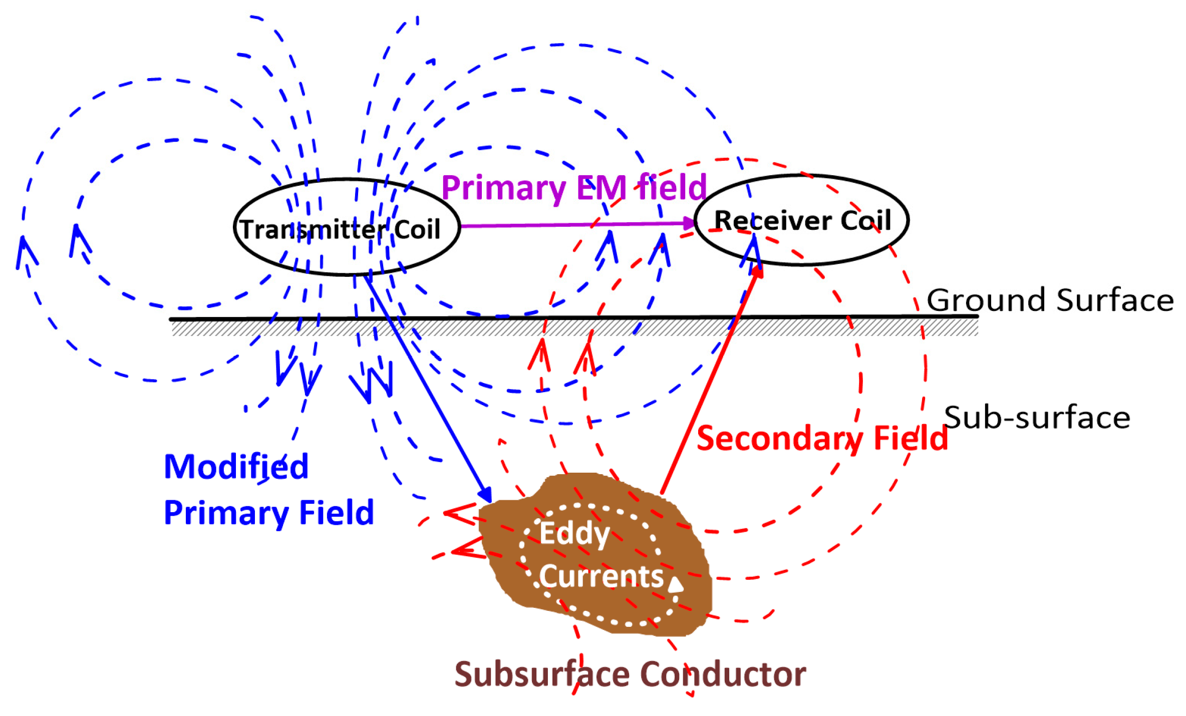
4.1. Basic Operating Principles of Electromagnetic Induction

The primary electromagnetic properties that the EMI sensor can determine are σ and µ. Therefore, without direct contact with the subsurface, EMI sensors measure the subsurface’s σa and apparent magnetic susceptibility (χa) [29,198]. Three pathways of current flows are responsible for the soil σa (see Section 3.2.3). The interpretation of σa is complex and based on several soil properties such as soil salinity, SWC, soil porosity, bulk density (compaction), SOM, CEC, clay content, and temperature [147,150,153,199,200,201,202].
σ increases with increasing temperature and is usually expressed at the reference temperature of 25 °C according to:
σ25 = ft × σt
ft = 0.4470 + 1.4034e(−t/26.815)
σ measured at an actual temperature t (σt) can be converted into the σ at 25 °C (σ25) [150,203]. In Equation (8), ft is the temperature conversion factor.
Initially, EMI was used to measure soil σ and subsequently to estimate other soil properties such as SWC, soil texture (mainly the clay content), bulk density, SOM, CEC, and soil pH [29,202].
An EMI sensor primarily consists of two coils: a Tx coil and an Rx coil (Figure 6). The Tx sends the time-varying or frequency-varying alternative current through a coil. This alternating current produces a time-varying primary magnetic field, which interacts with the conductive subsurface to induce eddy currents. These eddy currents generate the secondary EM field. The amplitude and phase of the primary magnetic field (Hp) and the secondary magnetic field (Hs) are received by the Rx coil [204] (Figure 6). The ratio of the Hs and Hp is proportional to the subsurface σa under low induction number conditions according to the equation [204]:
σ a = 4 ω μ 0 S 2 H s H p
where ω is the angular frequency, µo is the magnetic permeability of free space (4π × 10−7 H/m), and S is inter-coil spacing (m).
Although Equation (10) is the most widely used model for estimating the σ of soil from the EM field measurements, as it is implemented in commercially available sensors, it relies on a series of simplifications, and its application requires specific calibration.
Single-to-multi-coil (MC) and single-to-multi-frequency (MF) are the commercially available EMI sensors used in agricultural and environmental fields (Figure 7). MC and MF sensors have different depth-sensitivity functions and different footprints and, therefore, characterize different soil volumes (Figure 8). MC EMI sensors have different coil separations between the Tx coil (usually one) and Rx coils (usually two or three) with one operating frequency to explore different integrated depths. In MF EMI sensors, one Tx coil and one Rx coil operate with different frequencies (Figure 8). The depth of investigation of MF sensors increases with decreasing frequency [206,207].
Both MC and MF EMI sensors can operate in horizontal dipole (EMh) (vertical coplanar) and vertical dipole (EMv) (horizontal coplanar) orientations and give different integrated depths of investigations (DOI) in each dipole or coil orientation (Figure 9). The EMh DOI is approximately 0.75 times the inter-coil spacing, while the EMv DOI is about 1.5 times the inter-coil spacing [204]. Current flow paths under different coil orientations (EMh and EMv) differ. The DOI of EMI sensors depends on field condition (height of operation, soil σ, µ, and stratigraphy), operating frequency, type of the sensor (MC or MF), and coil orientation (EMh or EMv). Even though theoretical DOI is based on homogeneous soil conditions, the actual DOI under heterogeneous field conditions (due to changing physical and chemical properties) can vary [147,208].
Figure 8. Integral depth and sampling volume variation of (a) multi-coil (MC) and (b) multi-frequency (MF) electromagnetic induction (EMI) sensors (modified from Keiswetter & Won, [209]).
Remotesensing 15 02932 g008

4.2. Applications of Electromagnetic Induction in Soil Studies

This section discusses the main applications of EMI in estimating soil properties and states such as SWC, soil compaction, soil salinity, soil texture, and SOM.

4.2.1. Soil Salinity

The spatial and temporal variability of soil salinity in the agricultural landscape can be assessed and monitored using EMI sensors by measuring σa [210,211,212]. While some studies considered σa measured by EMI as a soil salinity indicator, others used σa to estimate actual soil salinity (e.g., σe) [212,213,214,215,216]. However, the applications of EMI have limitations. The conversion of EMI measured σa into soil salinity is complex and needs to use different models (such as Rhoades’ model (1976)) and regression equations [213,217,218]. Furthermore, EMI applications that estimate soil salinity require site-specific calibration [213,219,220].
Several studies have been carried out to estimate soil salinity’s spatial and temporal variation by developing simple regression models with σa. Diaz et al. [217] developed and compared two calibration methods, simple regression models derived from the design of the sensor: σa–σe and σa–σ1:5. The authors found that the σe estimations were more accurate when compared to the σ1:5 estimations using EMI measured σa. In another study by Doolittle et al. [218], simple linear regression (SLR) models were developed between σe measured in different depth intervals and σa measured using two different EMI instruments: EM38 (single frequency) and GEM300 (multi-frequency). Both instruments gave similar spatial and temporal variations, and in the 0–0.30 m depth interval, the coefficient of determination (R2) was >0.90 (p = 0.005) for both instruments [218]. Ganjegunte et al. [213] developed multiple linear regression (MLR) models to estimate the soil salinity (as σe) and sodium absorption ratio (SAR) in two study sites using σa. The authors found that the R2 values were 0.91 and 0.93 (p = 0.05) between the MLR model estimated and the measured σe, while the R2 values were 0.89 and 0.90 (p = 0.05) between the MLR model estimated and the measured SAR for two studied sites [213].
Geostatistical methods such as ordinary kriging are often applied to observe and predict the spatial and temporal variation of soil salinity using measured σa data [212,214,220]. A recent study researched variations in soil salinity using the time-lapse inversion of σa measured using an EMI sensor. The authors applied a 2D hydrological model, HYDRUS-2D [221], by considering water contents and solute concentrations. The authors found that correlation (r) between σa and σe was 0.88 (p = 0.001) and showed the reliability of the EMI method in measuring soil salinity in salt-water-irrigated areas [205].

4.2.2. Soil Water Content

SWC and σw play a significant role in contributing to the variation of σa. Early stage research studies mapped the spatial or temporal variation of σa and SWC to investigate the influence of SWC and soil water dynamics on σa [199,222]. Based on the findings by the above researchers, subsequent studies have developed site-specific relationships between σa and SWC [151,152,223,224]. The latest research improved the modeling approaches [225,226,227,228] to estimate the SWC from σa.
Kachanoski et al. [222] conducted a field-scale experiment to determine the relationships between spatial variations of σa, SWC, and soil texture in areas with low soluble salts. The authors found that the spatial variation of the measured SWC correlated with σa (R2 = 0.77). An additional experiment evaluated the impact of air and soil temperature, as well as shallow hydraulic conditions such as SWC and water table depth, on the spatial and temporal variation of σa, and the authors found that the σa was low under cold climatic conditions [199]. Additionally, the duration and intensity of rainfall and irrigation effects may influence the σa over a short period [199]. Using different soils, Brevick et al. [223] reported a linear relationship between σa and the SWC and found a significant impact of SWC on σa. Another study compared the spatial variability of σa under wet and dry conditions and evaluated the relationship between clay content and SWC [229]. The authors found significantly larger σa values during the wet days. The correlation between σa and SWC was found to be nearly two times greater in wet conditions (r = 0.54) than on dry days (r = 0.27) [229]. EMI surveys were also carried out to study σa variation under flood and drought (wetting and drying) conditions in a paddy field. Islam et al. [230] showed that flooding increased the stability of σa by reducing the micro-scale variability of σa due to the absence of soil moisture dynamics. The relationship between SWC and σa (MC and MF EMI sensors) was developed and evaluated in a managed podzolic soil [152]. Linear regression models were developed for SWC with MC and MF sensors separately. The authors found the highest predicting accuracy of SWC using σa measured by an MC EMI sensor (R2 = 0.79), rather than that of an MF sensor (R2 = 0.17) [152]. However, with a new calibration method, Robinet et al. [224] developed a non-linear relationship between SWC and σa measurements from an MC sensor for deeper depths, which was also influenced by σw.
Hezarjaribi and Sourell [231] used electrical resistivity and EMI techniques (EM-38) to develop site-specific relationships between σa and the total available water content within the upper 0.60 m of the soil profile. According to the developed relationships, the resistivity technique gave a higher correlation coefficient (R2 = 0.77) for the total available water content. In contrast, EMI provided a lower correlation coefficient (R2 = 0.56, and R2 = 0.35 for vertical and horizontal dipoles, respectively) [231]. However, Huth and Poulton [232] studied the soil water extraction pattern of a 0.90 m soil profile with σa and found a good correlation between SWC and σa (R2 = 0.93). Soil water distribution estimations in wheat [200] and cotton [233] fields were carried out using EMI sensors which showed an accurate estimation of SWC (R2 > 0.70) using σa measurements within the root zone. Altdorff et al. [151] determined the accuracy of the correlation between σa measured using an MC EMI sensor and SWC measured using TDR under different agronomic treatments (dairy manure, inorganic nitrogen, and phosphorous). The major finding of their study was that the σa–SWC correlation varied both spatially and temporally and was dependent on several soil properties, such as soil texture, bulk density, and site conditions, potentially due to the changes in ionic strength under different agronomic treatments [151].
Advanced electromagnetic models, combined with inversion techniques and multi-offset measurements, can be used to reconstruct vertical conductivity profiles from the EMI measurements of soil σa. This method allows for the estimation of the SWC at specific depths using mathematical models applied to the depth-specific σa values [225,226,227,228]. The spatiotemporal variability of SWC in irrigated maize fields was assessed using the probabilistic inversion of time-lapse σa data [225]. The authors showed that the time-lapse method is beneficial to use when identifying the spatiotemporal variability of the SWC and soil water dynamics [225]. In another study, σa related to SWC and potato tuber yield and established a two-layer model for σa with a mathematical model [226]. The least-square inversion algorithm was applied to determine the σa of soil layers to predict the SWC and spatiotemporal management zones during wet and dry conditions [228]. In this study, EMI-estimated SWC compared well with neutron probe measurements for wet and dry conditions, with Pearson correlations of 0.74 and 0.95, respectively [228].
No empirical or theoretical model or relationship has been developed to estimate SWC accurately from σa. The relationship between σa and SWC depends on several soil properties, states, and specific field conditions; thus, site-specific calibrations are required [234,235,236]. Site-specific empirical relationships between the SWC and σa are reported as being linear in most of the literature [201,223,236,237]. At the same time, a few studies have shown that the relationship changes to being non-linear when the variability of the SWC is high [222,224,234]. However, SWC maps could be developed using σa to understand the spatial and temporal variability pattern of the SWC, being correlated weakly, moderately, or strongly with σa [151,152,208,233,238,239,240,241].

4.2.3. Bulk Density and Soil Compaction

The potential of σa as a proxy to estimate the spatial and temporal variation of soil compaction/bulk density has been studied previously as σa is a function of soil compaction/bulk density [47]. Previous research showed that σa increases as soil compaction increases [242,243,244]. Galambošová et al. [244] evaluated the potential of the EMI method or sensors to determine the compacted and non-compacted areas in silty clay soils and observed higher σa values in compacted areas (r = 0.66) than in non-compacted areas [244]. Al-Gaadi et al. [245] evaluated the potential of σa measured from EMI to estimate soil compaction by considering the influence of SWC. The authors found that σa measurement can predict soil compaction under low SWC conditions (below 7%) in sandy soil [245].
Besson et al. [246] discovered no clear correlation between soil compaction and σa in newly plowed land due to significant variation in soil properties such as SWC. A recent study also found that there was no good correlation between σa with bulk density and penetration resistance, even though the study showed a positive correlation (r = 0.61) between σa and clay content [247]. The authors suggested that the variability in clay content covers comparatively slight variation effects of soil compaction, and that subsurface heterogeneity (due to stones) would also affect σa measurements [247].

4.2.4. Other Soil Properties

Other than SWC, soil salinity, and compaction, σa measured using EMI has been used to estimate and map the spatial and temporal variation of soil texture and clay content [201,229,247,248,249,250,251], SOM or SOC [191,201,248,249,251,252], CEC [250], and soil pH [248,249,251].

4.2.5. Apparent Magnetic Susceptibility

Most EMI applications in soil studies are related to σa measurements; however, χa also has the potential to be used in relation to soil properties and processes. However, very few soil studies have been conducted using χa (in-phase data), which is simultaneously measured by commonly available EMI sensors. The χa of soil is determined by the number of magnetic minerals present and is primarily controlled by magnetite and maghemite concentrations [253]. Similar to σa, χa is also influenced by soil layering, porosity, saturation, texture, SOM, and natural and anthropogenic features [254,255,256]. Using metal targets, Sadatcharam et al. [254] studied the depth sensitivity of χa using MC and MF EMI sensors. Shirzaditabar and Heck [256] studied soil drainage characteristics of soil profiles using χa under different drainage conditions; the authors found that the χa values in poorly drained soil profiles were lower than in well-drain soil profiles. McLachlan et al. [257] studied physicochemical properties, such as SOM, nitrogen, CEC, and pH, using both σa and χa, reporting a potential relationship between χa and CEC and SOM.
In soil studies related to agriculture, the EMI method is used in various applications. Based on the influence of several soil properties and states of σa, the relationships with interrelated soil properties are complex. Additionally, the use of the EMI method provides σa and χa simultaneously; therefore, the application range in soil studies can be expanded with future research.

5. Synthesis and Critical Analysis

According to the literature reviewed in soil studies, many studies have focused on estimating soil properties and states using GPR and EMI individually. Figure 10 shows the number of studies conducted using GPR and EMI techniques from 1995 to 2022. This analysis considered the five most widely assessed soil properties and states: SWC, soil salinity, soil compaction, soil texture/clay content, and SOM/SOC. Overall, SWC is the soil state most assessed using GPR (>600 studies, 85.17%) and using EMI (>100 studies, 42.09%), as shown in Figure 10 and Figure 11. Compared to GPR, there are many soil salinity studies present in the literature which used the EMI technique, which is as expected, since the EMI instrument measures the soil σa, which is considered to be a conductivity meter. Figure 10 clearly highlights the lack of studies concerning other vital properties such as soil compaction, soil texture, and SOM using either method.
Figure 11 shows the percentages of studies of each soil property and state using GPR (Figure 11a) and using EMI (Figure 11b) that were conducted from 1995 to 2022. For the GPR method, most studies that were conducted were related to SWC, and studies that were related to other soil properties and states accounted for less than 15% (Figure 11a). On the other hand, higher percentages of studies have been carried out which assess the two properties of SWC (40.29%) and soil salinity (34.86%) using the EMI technique (Figure 11b). Furthermore, Figure 11 clearly shows that the EMI technique has been used in the literature to cover a wide range of soil properties (e.g., SWC, salinity, soil texture/clay content, and SOM/SOC), unlike the GPR technique. The high-occurrence keywords and their concomitant links related to soil studies conducted using the GPR and EMI techniques during the past 15 years (2007–2022) are shown in the term maps (Figure 12). With respect to the use of the GPR technique, “SWC > εr > TDR > vadose zone > hydro-geophysics” are the five most cited keywords (Figure 12a), while those for the EMI technique are “σ > σa > SWC > soil salinity > Irrigation” (Figure 12b).
Not many studies have been carried out combining the GPR and EMI techniques to estimate soil properties and states. Toy et al. [258] compared EMI and GPR measurements (σa and GPR velocity) of the SWC of three different soil textures: sand, sandy loam, and silt loam. The authors found that the velocity variation of GPR DGW was more sensitive to the SWC variation than the σa variation. In all three sites, the σa measurements of EMh correlated well with the DGW velocity, since the DOI is shallow in EMh. Furthermore, among these three sites, both instruments performed well regarding the silt loam site [258]. De Benedetto et al. [185] mapped the spatial variation of clay by integrating GPR, EMI, and geostatistical techniques. In this study, the authors applied EMI to assess the soil texture and GPR to detect the soil horizons. Additionally, the spatial variation of SWC was studied by combining GPR data and EMI data with geostatistical techniques. The authors found that data from GPR and EMI could be used as auxiliary variables to estimate the SWC through geostatistical techniques [30,259]. The reviewed literature emphasizes the importance of the integration of EMI and GPR data and geostatistical techniques in the estimation of the spatial and temporal variation of soil properties such as SWC, clay content, and SOM/SOC to provide the information needed to support PA [185,191,259]. Jonard et al. [143] showed the potential of GPR and EMI techniques to evaluate the effect of different tillage practices, including conventional tillage, deep loosening tillage, and reduced tillage on SWC. Moghadas et al. [260] analyzed the full-wave joint inversion of GPR and EMI data for reconstructing two-layered soil. Several inversion strategies were studied, including data fusion methods and sequential inversion, and the complementarities between GPR and EMI were illustrated and discussed using objective function plots.
Previous studies in the literature show that both GPR and EMI methods have advantages and disadvantages when it comes to soil studies (Table 3). GPR is commonly used for estimating SWC because the relationship between εr and SWC is not significantly influenced by other factors, resulting in relatively accurate estimations. On the other hand, EMI has a broader range of applications compared to GPR, because σa measured by EMI is affected by multiple factors, as mentioned above. However, the effective use of EMI for estimating soil properties and states necessitates site-specific calibrations to be conducted. Nevertheless, even in the absence of such calibrations, EMI has demonstrated its usefulness as a valuable tool for mapping distinct soil units and delineating management zones. Regarding other soil properties, GPR is still in the early stages of application development. EMI has been shown to work well in clayey soils, whereas GPR is more suitable for low-conductive soils. Researchers have reported that GPR data necessitate more sophisticated data processing and interpretations than EMI. The additional limitations of GPR include its high capital costs and the need for highly skilled personnel to operate it and interpret/analyze the data.

6. Summary and Future Directions

Ground-penetrating radar (GPR) and electromagnetic induction (EMI) have been successfully applied in soil studies to assess various soil properties and their spatial and temporal variability. Compared to traditional methods, the non-destructive nature of GPR and EMI offers several advantages in terms of their application to the agricultural landscape, such as their ability to make repeated measurements, save on labor, and provide more extensive spatial coverage (in terms of both vertical and horizontal spatial variability) with geo-referenced data. Compared to the traditional point scale measurements, GPR and EMI applications in soil studies have a larger sampling volume (including a higher penetration depth and wider footprint), which is primarily controlled by the frequency, antenna separation, and coil orientation. Thus, mapping soil proxies related to EMI (apparent electrical conductivity: σa) and GPR (dielectric permittivity: εr) techniques in the agricultural landscape can predict and map the spatiotemporal variability of soil properties and states. The possession of this information is fundamental to obtain the information required to determine the management zones in support of precision agriculture (PA), where the application rate, amount, and timing of the agricultural inputs and their management can be optimized.
Soil water content (SWC) and electrical conductivity (σ) are the two main soil parameters influencing GPR and EMI proxies. GPR is widely used for SWC estimation and is well-established with different data collection and processing methods; these include direct ground wave velocity, reflected wave velocity, transillumination method, and full waveform inversion, and their application to different soil types under different conditions. The application of EMI is comparatively broad as it has been tested for estimating SWC, soil salinity, and a few other properties. Furthermore, some EMI studies have considered several interrelated soil properties and states at the same time. The estimation of other soil properties such as soil compaction, soil texture/clay content, soil organic matter/soil organic carbon, soil pH, and cation exchange capacity, in addition to soil hydraulic properties such as water holding capacity, infiltration capacity, water repellency, and hydraulic conductivity, using both techniques is therefore warranted. Additionally, the responses of GPR and EMI techniques are favored for different soil properties, even though all these properties are directly or indirectly related to each other. Future directions of EMI and GPR require a focus on the estimation and mapping of many soil properties simultaneously within the agricultural landscape to support applications in PA.
For example, the influence of different soil properties on EM field strengths (EMI) and wave propagation (GPR) under heterogeneous and variable soil conditions such as alternate wetting and drying, plowing and compaction, and high and low saline conditions should be investigated. Most research studies on advancing data analysis and the interpretation of these two techniques have been conducted under control conditions and through modeling approaches by only considering one or a few variables at a time. However, when it comes to the actual field application of these two techniques, the situation is more complex and heterogeneous under natural and managed conditions. Thus, the combined effect of different soil properties and states on the proxies of GPR and EMI should be further investigated under variable field conditions. This approach will provide the necessary information to enhance the prediction accuracy of soil properties and states and their variability in both spatial and temporal scales within the agricultural landscape. Prediction accuracy can be further enhanced using advanced modeling approaches such as artificial intelligence by incorporating heterogeneous (both temporally stable and variable) field conditions.
The main disadvantages of these two techniques are the difficulty of the real-time data processing and interpretation of most of the properties. However, advanced, computer-based commercial solutions are progressively becoming available, such as gprSense (http://www.gprsense.com, accessed on 26 December 2022) for real-time GPR full-wave inversion, in addition to SWAT (soil, water, and topography) maps (https://swatmaps.com, accessed on 25 March 2023) for agronomic decision-making in agricultural landscapes, such as that regarding variable-rate fertilizer, seed, soil amendment, pesticide applications, and precision water management. Both the GPR and EMI techniques are EM techniques, even though the operating principles of the techniques are quite different. Therefore, integrating these two techniques can provide the information needed to advance the PA by assessing several soil properties at once by amending the negative aspect of one technique with that of the other. Thus, the future direction of EMI and GPR applications in soil studies to support PA needs to focus on research questions for potential integration by considering both techniques’ similarities, differences, and advantages and disadvantages.

Author Contributions

Conceptualization, S.P. and L.G.; methodology, S.P., S.L. and L.G.; software, S.P.; validation, S.L., M.C., M.K., C.S. and L.G.; formal analysis, S.P.; investigation, S.P.; data curation, S.P. and S.L.; writing—original draft preparation, S.P.; writing—review and editing, S.L., M.C., M.K., C.S. and L.G.; visualization, S.P., S.L. and L.G.; supervision, L.G., C.S., S.L. and M.C.; project administration, L.G.; funding acquisition, L.G. All authors have read and agreed to the published version of the manuscript.

Funding

This research was funded by Natural Sciences and Engineering Research Council of Canada, Discovery Grant (NSERC-DG): RGPIN-2019-04614, Industry, Energy and Innovation of the Government of Newfoundland and Labrador, IET Grant: 5404-1962-102, and Grenfell Campus, Memorial University of Newfoundland.

Data Availability Statement

The data used in this review is the list of cited publications.

Conflicts of Interest

The authors declare no conflict of interest.

References

  1. Bongiovanni, R.; Lowenberg-DeBoer, J. Precision agriculture and sustainability. Precis. Agric. 2004, 5, 359–387. [Google Scholar] [CrossRef]
  2. Aubert, B.A.; Schroeder, A.; Grimaudo, J. IT as enabler of sustainable farming: An empirical analysis of farmers’ adoption decision of precision agriculture technology. Decis. Support Syst. 2012, 54, 510–520. [Google Scholar] [CrossRef] [Green Version]
  3. Shafi, U.; Mumtaz, R.; García-Nieto, J.; Hassan, S.A.; Zaidi, S.A.R.; Iqbal, N. Precision agriculture techniques and practices: From considerations to applications. Sensors 2019, 19, 3796. [Google Scholar] [CrossRef] [Green Version]
  4. Goel, R.K.; Yadav, C.S.; Vishnoi, S.; Rastogi, R. Smart agriculture—Urgent need of the day in developing countries. Sustain. Comput. Inform. Syst. 2021, 30, 100512. [Google Scholar] [CrossRef]
  5. Xia, Y.; Zhang, M.; Tsang, D.C.W.; Geng, N.; Lu, D.; Zhu, L.; Igalavithana, A.D.; Dissanayake, P.D.; Rinklebe, J.; Yang, X.; et al. Recent advances in control technologies for non-point source pollution with nitrogen and phosphorous from agricultural runoff: Current practices and future prospects. Appl. Biol. Chem. 2020, 63, 8. [Google Scholar] [CrossRef]
  6. Stafford, J.V. Implementing precision agriculture in the 21st century. J. Agric. Eng. Res. 2000, 76, 267–275. [Google Scholar] [CrossRef] [Green Version]
  7. Becker, S.M.; Franz, T.E.; Abimbola, O.; Steele, D.D.; Flores, J.P.; Jia, X.; Scherer, F.T.; Rudnick, R.D.; Neale, C.M. Feasibility assessment on use of proximal geophysical sensors to support precision management. Vadose Zone J. 2022, 21, e20228. [Google Scholar] [CrossRef]
  8. Friedl, M.A. Remote sensing of croplands. In Comprehensive Remote Sensing—Elsevier Earth Systems and Environmental Science; Liang, S., Ed.; Elsevier: Amsterdam, The Netherlands, 2018; Volume 6, pp. 78–95. [Google Scholar] [CrossRef]
  9. Pallottino, F.; Biocca, M.; Nardi, P.; Figorilli, S.; Menesatti, P.; Costa, C. Science mapping approach to analyze the research evolution on precision agriculture: World, EU and Italian situation. Precis. Agric. 2018, 19, 1011–1026. [Google Scholar] [CrossRef]
  10. Nicol, L.A.; Nicol, C.J. Adoption of precision agriculture to reduce inputs, enhance sustainability and increase food production: A study of Southern Alberta, Canada. WIT Trans. Ecol. Environ. 2018, 217, 1743–3541. [Google Scholar] [CrossRef] [Green Version]
  11. Hammond, M.W.; Mulla, D.J.; Fairchild, D.S. Development of management maps for soil variability. In Proceedings of the 39th Annual Far West Regional Fertilizer Conference, Bozeman, MT, USA, 11–13 July 1988; pp. 67–76. [Google Scholar]
  12. Mulla, D.J.; Hammond, M.W. Mapping of soil test results from large irrigation circles. In Proceedings of the 39th Annual Far West Regional Fertilizer Conference, Bozeman, MT, USA, 11–13 July 1988; pp. 169–176. [Google Scholar]
  13. Schmidhalter, U.; Maidl, F.X.; Heuwinkel, H.; Demmel, M.; Auernhammer, H.; Noack, P.O.; Rothmund, M. Precision farming–adaptation of land use management to small scale heterogeneity. In Perspectives for Agroecosystem Management: Balancing Environmental and Socio-Economic Demands; Schröder, P., Pfadenhauer, J., Munch, J.C., Eds.; Elsevier: Amsterdam, The Netherlands, 2008; Chapter 2.3; pp. 121–199. [Google Scholar] [CrossRef]
  14. Pinaki, M.; Tewari, V.K. Present status of precision farming: A review. Int. J. Agric. Res. 2010, 5, 1124–1133. [Google Scholar] [CrossRef] [Green Version]
  15. Mulla, D.; Khosla, R. Historical evolution and recent advances in precision farming. In Soil Specific Farming: Precision Agriculture; Lal, R., Stewart, B.A., Eds.; Taylor and Francis: Boca Raton, FL, USA, 2015; Chapter 1; pp. 1–36. [Google Scholar]
  16. Alix, A.; Capri, E. Modern agriculture in Europe and the role of pesticides. In Advances in Chemical Pollution, Environmental Management and Protection; Capri, E., Alix, A., Eds.; Elsevier: Amsterdam, The Netherlands, 2018; Volume 2, pp. 1–22. [Google Scholar] [CrossRef]
  17. Kashyap, B.; Kumar, R. Sensing methodologies in agriculture for soil moisture and nutrient monitoring. IEEE Access 2021, 9, 14095–14121. [Google Scholar] [CrossRef]
  18. Hammond, M.W.; Mulla, D.J. Field variation in soil fertility: Its assessment and management for potato production. In Proceedings of the 28th Annual Washington State Potato Conference, Moses Lake, WA, USA, 2 February 1989. [Google Scholar]
  19. Jarolímek, J.; Stočes, M.; Masner, J.; Vaněk, J.; Šimek, P.; Pavlík, J.; Rajtr, J. User-technological index of precision agriculture. Agris On-Line Pap. Econ. 2017, 9, 69–75. [Google Scholar] [CrossRef] [Green Version]
  20. Fairchild, D.; Hammond, M. Using computerized fertilizer application equipment for efficient soil fertility management. In Proceedings of the 39th Annual Regional Fertilizer Conference, BoTeman, MT, USA, 11–13 July 1988; Jacobsen, J.S., Ed.; pp. 77–82. [Google Scholar]
  21. Mulla, D.J. Using geostatistics and spectral analysis to study spatial patterns in the topography of southeastern Washington State, U.S.A. Earth Surf. Process. 1988, 13, 389–405. [Google Scholar] [CrossRef]
  22. Vereecken, H.; Binley, A.; Cassiani, G.; Revil, A.; Titov, K. Applied hydrogeophysics. In Applied Hydrogeophysics: NATO Science Series; Vereecken, H., Binley, A., Cassiani, G., Revil, A., Titov, K., Eds.; Springer Dordrecht: Berlin, Germany, 2006; Volume 71, pp. 1–8. [Google Scholar] [CrossRef]
  23. Rubin, Y.; Hubbard, S.S. Hydrogeophysics; Springer: Cham, Switzerland, 2005; Volume 50. [Google Scholar] [CrossRef]
  24. Lambot, S.; Binley, A.; Slob, E.C.; Hubbard, S. Foreword to the special issue on ground-penetrating radar in hydrogeophysics. Vadose Zone J. 2008, 7, 137–139. [Google Scholar] [CrossRef] [Green Version]
  25. Binley, A.; Cassiani, G.; Deiana, R. Hydrogeophysics: Opportunities and challenges. Boll. Geofis. Teor. Ed Appl. 2010, 51, 267–284. [Google Scholar]
  26. Vereecken, H.; Hubbard, S.; Binley, A.; Ferre, T. Hydrogeophysics: An introduction from the guest editors. Vadose Zone J. 2004, 3, 1060–1062. [Google Scholar] [CrossRef]
  27. Blazevic, L.A.; Bodet, L.; Pasquet, S.; Linde, N.; Jougnot, D.; Longuevergne, L. Time-lapse seismic and electrical monitoring of the vadose zone during a controlled infiltration experiment at the Ploemeur hydrological observatory, France. Water 2020, 12, 1230. [Google Scholar] [CrossRef]
  28. Hubbard, S.S. Hydrogeophysics; Lawrence Berkeley National Laboratory: Berkeley, CA, USA, 2011. [Google Scholar]
  29. Doolittle, J.A.; Brevik, E.C. The use of electromagnetic induction techniques in soils studies. Geoderma 2014, 223–225, 33–45. [Google Scholar] [CrossRef] [Green Version]
  30. De Benedetto, D.; Montemurro, F.; Diacono, M. Mapping an agricultural field experiment by electromagnetic Induction and ground penetrating radar to improve soil water content estimation. Agronomy 2019, 9, 638. [Google Scholar] [CrossRef] [Green Version]
  31. Slob, E.; Sato, M.; Olhoeft, G. Surface and borehole ground-penetrating-radar developments. Geophysics 2010, 75, 75A103–75A120. [Google Scholar] [CrossRef] [Green Version]
  32. Zajícová, K.; Chuman, T. Application of ground penetrating radar methods in soil studies: A review. Geoderma 2019, 343, 116–129. [Google Scholar] [CrossRef]
  33. Huisman, J.A.; Hubbard, S.S.; Redman, J.D.; Annan, A.P. Measuring soil water content with ground penetrating radar: A review. Vadose Zone J. 2003, 2, 476–491. [Google Scholar] [CrossRef]
  34. van Dam, R.L. Calibration functions for estimating soil moisture from GPR dielectric constant measurements. Commun. Soil Sci. Plant Anal. 2014, 45, 392–413. [Google Scholar] [CrossRef]
  35. Liu, X.; Chen, J.; Cui, X.; Liu, Q.; Cao, X.; Chen, X. Measurement of soil water content using ground penetrating radar: A review of current methods. Int. J. Digit. Earth 2017, 12, 95–118. [Google Scholar] [CrossRef]
  36. Klotzsche, A.; Jonard, F.; Looms, M.C.; van der Kruk, J.; Huisman, J.A. Measuring soil water content with ground penetrating radar: A decade of progress. Vadose Zone J. 2018, 17, 1–9. [Google Scholar] [CrossRef] [Green Version]
  37. Zhang, M.; Feng, X.; Bano, M.; Xing, H.; Wang, T.; Liang, W.; Zhou, H.; Dong, Z.; An, Y.; Zhang, Y. Review of ground penetrating radar applications for water dynamics studies in unsaturated zone. Remote Sens. 2022, 14, 5993. [Google Scholar] [CrossRef]
  38. Olhoeft, G.R. Electrical, magnetic, and geometric properties that determine ground penetrating radar performance. In Proceedings of the 7th International Conference on Ground Penetrating Radar, The University of Kansas, Lawrence, KS, USA, 27–30 May 1998; pp. 177–182. [Google Scholar]
  39. Annan, A.P. Ground Penetrating Radar Principles, Procedures, and Applications; Workshop Notes, Sensors and Software Inc.: Mississauga, ON, Canada, 2004. [Google Scholar]
  40. Annan, A.P. Electromagnteic principles of ground penetrating radar. In Ground Penetrating Radar Theory and Applications; Jol, H.M., Ed.; Elsevier: Amsterdam, The Netherlands, 2009; pp. 3–37. [Google Scholar] [CrossRef]
  41. Weiler, K.W.; Steenhuis, T.S.; Boll, J.; Kung, K.J.S. Comparison of ground penetrating radar and time-domain reflectometry as soil water sensors. Soil Sci. Soc. Am. J. 1998, 62, 1237–1239. [Google Scholar] [CrossRef]
  42. Topp, G.C.; Davis, J.L.; Annan, A.P. Electromagnetic determination of soil water content: Measurements in coaxial transmission lines. Water Resour. Res. 1980, 16, 574–582. [Google Scholar] [CrossRef] [Green Version]
  43. Turesson, A. Water content and porosity estimated from ground-penetrating radar and resistivity. J. Appl. Geophy. 2006, 58, 99–111. [Google Scholar] [CrossRef]
  44. Roth, K. Calibration of time domain reflectometry for water content measurement using a composite dielectricity approach. Water Resour. Res. 1990, 26, 2267–2273. [Google Scholar] [CrossRef]
  45. White, I.; Knight, J.H.; Zegelin, S.J.; Topp, G.C. Comments on ‘Considerations on the use of time-domain reflectometry (TDR) for measuring soil water content’ by W. R. Whalley. Eur. J. Soil Sci. 1994, 45, 503–508. [Google Scholar] [CrossRef]
  46. Wanniarachchi, D.; Cheema, M.; Thomas, R.; Galagedara, L. Effect of biochar on TDR-based volumetric soil moisture measurements in a loamy sand podzolic soil. Soil Syst. 2019, 3, 49. [Google Scholar] [CrossRef] [Green Version]
  47. Archie, G.E. The electrical resistivity log as an aid in determining some reservoir characteristics. Trans. Am. Inst. Min. 1942, 146, 54–62. [Google Scholar] [CrossRef]
  48. Shah, P.H.; Singh, D.N. Generalized archie’s law for estimation of soil electrical conductivity. J. ASTM Int. 2005, 2, 145–164. [Google Scholar]
  49. Ewing, R.P.; Hunt, A.G. Dependence of the electrical conductivity on saturation in real porous media. Vadose Zone J. 2006, 5, 731–741. [Google Scholar] [CrossRef]
  50. Glover, P.W.J. A generalized Archie’s law for n phases. Geophysics 2010, 75, 247–265. [Google Scholar] [CrossRef] [Green Version]
  51. Glover, P.W.J. Archie’s law—A reappraisal. Solid Earth 2016, 7, 1157–1169. [Google Scholar] [CrossRef] [Green Version]
  52. Birchak, J.R.; Gardner, C.G.; Hipp, J.E.; Victor, J.M. High dielectric constant microwave probes for sensing soil moisture. Proc. IEEE 1974, 62, 93–98. [Google Scholar] [CrossRef]
  53. Lai, W.L.; Tsang, W.F.; Fang, H.; Xiao, D. Experimental determination of bulk dielectric properties and porosity of porous asphalt and soils using GPR and a cyclic moisture variation technique. Geophysics 2006, 71, K93. [Google Scholar] [CrossRef]
  54. Mount, G.J.; Comas, X. Estimating porosity and solid dielectric permittivity in the Miami Limestone using high-frequency ground penetrating radar (GPR) measurements at the laboratory scale. Water Resour. Res. 2014, 50, 7590–7605. [Google Scholar] [CrossRef]
  55. Zadhoush, H.; Giannopoulos, A.; Giannakis, I. Optimising the complex refractive index model for estimating the permittivity of heterogeneous concrete models. Remote Sens. 2021, 13, 723. [Google Scholar] [CrossRef]
  56. Rhoades, J.D.; Raats, P.A.C.; Prather, R.J. Effects of liquid-phase electrical conductivity, water content, and surface conductivity on bulk soil electrical conductivity. Soil Sci. Soc. Am. J. 1976, 40, 651–655. [Google Scholar] [CrossRef]
  57. Baker, G.S.; Jordan, T.E.; Pardy, J. An introduction to ground penetrating radar (GPR). In Stratigraphic Analyses Using GPR; Baker, G.S., Jol, H.M., Eds.; Geological Society of America: Boulder, CO, USA, 2007; Volume 432, pp. 1–18. [Google Scholar] [CrossRef]
  58. Davis, J.L.; Annan, A.P. Ground penetrating radar for high-resolution mapping of soil and rock stratigraphy. Geophys. Prospect. 1989, 37, 531–551. [Google Scholar] [CrossRef]
  59. Reynolds, J.M. An Introduction to Applied and Environmental Geophysics, 2nd ed.; A John Wiley & Sons Ltd.: West Sussex, UK, 2011. [Google Scholar]
  60. Knight, R. Ground penetrating radar for environmental applications. Annu. Rev. Earth Planet. Sci. 2001, 29, 229–255. [Google Scholar] [CrossRef] [Green Version]
  61. Annan, A.P. Ground penetrating radar. In Near-Surface Geophysics; Butler, D.K., Ed.; Society of Exploration Geophysics: Tulsa, OK, USA, 2005; pp. 434–557. [Google Scholar] [CrossRef]
  62. Cassidy, N.J. Electrical and magnetic properties of rocks, soils, fluids. In Ground Penetrating Radar Theory and Applications; Jol, H.M., Ed.; Elsevier: Amsterdam, The Netherlands, 2009; Chapter 2; pp. 41–67. [Google Scholar] [CrossRef]
  63. Sperl, C. Determination of Spatial and Temporal Variation of the Soil Water Content in an Agro-Ecosystem with Ground-Penetrating Radar. Ph.D. Thesis, Technische Universitat München, Munich, Germany, 1999. [Google Scholar]
  64. Lambot, S.; Rhebergen, J.; van den Bosch, I.; Slob, E.C.; Vanclooster, M. Measuring the soil water content profile of a sandy soil with an off-ground monostatic ground penetrating radar. Vadose Zone J. 2004, 3, 1063–1071. [Google Scholar] [CrossRef]
  65. Zhang, J.; Lin, H.; Doolittle, J. Soil layering and preferential flow impacts on seasonal changes of GPR signals in two contrasting soils. Geoderma 2014, 213, 560–569. [Google Scholar] [CrossRef]
  66. Chew, W.C. Waves and Fields in Inhomogeneous Media; Wiley-IEEE Press: Piscataway, NJ, USA, 1995. [Google Scholar]
  67. Galagedara, L.W.; Parkin, G.W.; Redman, J.D. An analysis of the ground penetrating radar direct ground wave method for soil water content measurement. Hydrol. Process. 2003, 17, 3615–3628. [Google Scholar] [CrossRef]
  68. Galagedara, L.W.; Parkin, G.W.; Redman, J.D.; Endres, A.L. Assessment of soil moisture content measured by borehole GPR and TDR under transient irrigation and drainage. J. Environ. Eng. Geophys. 2003, 8, 77–86. [Google Scholar] [CrossRef]
  69. Wijewardana, Y.G.N.S.; Galagedara, L.W. Estimation of spatio-temporal variability of soil water content in agricultural fields with ground penetrating radar. J. Hydrol. 2010, 391, 24–33. [Google Scholar] [CrossRef]
  70. Chanzy, A.; Tarussov, A.; Bonn, F.; Judge, A. Soil water content determination using a digital ground penetrating radar. Soil Sci. Soc. Am. J. 1996, 60, 1318–1326. [Google Scholar] [CrossRef]
  71. van Overmeeren, R.A.; Sariowan, S.V.; Gehrels, J.C. Ground penetrating radar for determining volumetric soil water content; results of comparative measurements at two test sites. J. Hydrol. 1997, 197, 316–338. [Google Scholar] [CrossRef]
  72. Hubbard, S.; Grote, K.; Rubin, Y. Mapping the volumetric soil water content of a california vineyard using high-frequency GPR ground wave data. Lead. Edge 2002, 21, 552. [Google Scholar] [CrossRef]
  73. Huisman, J.A.; Bouten, W. Accuracy and reproducibility of mapping surface soil water content with the ground wave of ground-penetrating radar. J. Environ. Eng. Geophys. 2003, 8, 67–75. [Google Scholar] [CrossRef]
  74. Galagedara, L.W.; Parkin, G.W.; Redman, J.D.; Von Bertoldi, P.; Endres, A.L. Field studies of the GPR ground wave method for estimating soil water content during irrigation and drainage. J. Hydrol. 2005, 301, 182–197. [Google Scholar] [CrossRef]
  75. Galagedara, L.W.; Parkin, G.W.; Redman, J.D. Measuring and modeling of direct ground wave depth penetration under transient soil moisture conditions. Subsurf. Sens. Technolo. Appli. 2005, 6, 193–205. [Google Scholar] [CrossRef]
  76. Illawathure, C.; Parkin, G.; Lambot, S.; Galagedara, L. Evaluating soil moisture estimation from ground-penetrating radar hyperbola fitting with respect to a systematic time-domain reflectometry data collection in a boreal podzolic agricultural field. Hydrol. Process. 2020, 34, 1428–1445. [Google Scholar] [CrossRef]
  77. Grote, K.; Hubbard, S.; Rubin, Y. Field-scale estimation of volumetric water content using ground penetrating radar ground wave techniques. Water Resour. Res. 2003, 39, 1–14. [Google Scholar] [CrossRef] [Green Version]
  78. Wollschläger, U.; Roth, K. Estimation of temporal changes of volumetric soil water content from ground-penetrating radar reflections. Subsurf. Sens. Technol. Appli. 2005, 6, 207–218. [Google Scholar] [CrossRef]
  79. Lu, Y.; Song, W.; Lu, J.; Wang, X.; Tan, Y. An examination of soil moisture estimation using ground penetrating radar in desert steppe. Water 2017, 9, 521. [Google Scholar] [CrossRef] [Green Version]
  80. Lunt, I.A.; Hubbard, S.S.; Rubin, Y. Soil moisture content estimation using ground-penetrating radar reflection data. J. Hydrol. 2005, 307, 254–269. [Google Scholar] [CrossRef]
  81. Ercoli, M.; Di Matteo, L.; Pauselli, C.; Mancinelli, P.; Frapiccini, S.; Talegalli, L.; Cannata, A. Integrated GPR and laboratory water content measures of sandy soils: From laboratory to field scale. Constr. Build. Mater. 2018, 159, 734–744. [Google Scholar] [CrossRef]
  82. Stoffregen, H.; Zenker, T.; Wessolek, G. Accuracy of soil water content measurements using ground penetrating radar: Comparison of ground penetrating radar and lysimeter data. J. Hydrol. 2002, 267, 201–206. [Google Scholar] [CrossRef]
  83. Loeffler, O.; Bano, M. Ground penetrating radar measurements in a controlled vadose zone: Influence of the water content. Vadose Zone J. 2004, 3, 1082–1092. [Google Scholar] [CrossRef]
  84. Zhou, L.; Yu, D.; Wang, Z.; Wang, X. Soil water content estimation using high-frequency ground penetrating radar. Water 2019, 11, 1036. [Google Scholar] [CrossRef] [Green Version]
  85. Cui, X.; Guo, L.; Chen, J.; Chen, X.; Zhu, X. Estimating tree-root biomass in different depths using ground-penetrating radar: Evidence from a controlled experiment. IEEE Trans. Geosci. Remote Sens. 2019, 51, 3410–3423. [Google Scholar] [CrossRef]
  86. Liu, X.; Cui, X.; Guo, L.; Chen, J.; Li, W.; Yang, D.; Cao, X.; Chen, X.; Liu, Q.; Lin, H. Non-invasive estimation of root zone soil moisture from coarse root reflections in ground-penetrating radar images. Plant Soil 2019, 436, 623–639. [Google Scholar] [CrossRef]
  87. Sham, J.F.C.; Lai, W.W.-L.; Leung, C.H.C. Effects of homogeneous/heterogeneous water distribution on GPR wave velocity in a soil’s wetting and drying process. In Proceedings of the 16th International Conference on Ground Penetrating Radar, Hong Kong, China, 13–16 June 2016; IEEE: Manhattan, NY, USA, 2016; pp. 1–6. [Google Scholar] [CrossRef]
  88. Steelman, C.M.; Endres, A.L. Assessing vertical soil moisture dynamics using multi-frequency GPR common-midpoint soundings. J. Hydrol. 2012, 436–437, 51–66. [Google Scholar] [CrossRef]
  89. Huisman, J.A.; Sperl, C.; Bouten, W.; Verstraten, J.M. Soil water content measurements at different scales: Accuracy of time domain reflectometry and ground-penetrating radar. J. Hydrol. 2001, 245, 48–58. [Google Scholar] [CrossRef]
  90. Huisman, J.A.; Snepvangers, J.J.J.C.; Bouten, W.; Heuvelink, G.B.M. Monitoring temporal development of spatial soil water content variation: Comparison of ground penetrating radar and time domain reflectometry. Vadose Zone J. 2003, 2, 519–529. [Google Scholar] [CrossRef]
  91. Huisman, J.A.; Snepvangers, J.J.J.C.; Bouten, W.; Heuvelink, G.B.M. Mapping spatial variation in surface soil water content: Comparison of ground-penetrating radar and time domain reflectometry. J. Hydrol. 2002, 269, 194–207. [Google Scholar] [CrossRef]
  92. Grote, K.; Anger, C.; Kelly, B.; Hubbard, S.; Rubin, Y. Characterization of soil water content variability and soil texture using GPR groundwave techniques. J. Environ. Eng. Geophys. 2010, 15, 93–110. [Google Scholar] [CrossRef] [Green Version]
  93. Minet, J.; Bogaert, P.; Vanclooster, M.; Lambot, S. Validation of ground penetrating radar full-waveform inversion for field scale soil moisture mapping. J. Hydrol. 2012, 424, 112–123. [Google Scholar] [CrossRef] [Green Version]
  94. Ardekani, M.R.M. Off- and on-ground GPR techniques for field-scale soil moisture mapping. Geoderma 2013, 200–201, 55–66. [Google Scholar] [CrossRef]
  95. Thitimakorn, T.; Kummode, S.; Kupongsak, S. Determination of spatial and temporal variations of volumetric soil water content using ground penetrating radar: A case study in Thailand. Appl. Environ. Res. 2016, 38, 33–46. [Google Scholar] [CrossRef]
  96. Cao, Q.; Song, X.; Wu, H.; Gao, L.; Liu, F.; Yang, S.; Zhang, G. Mapping the response of volumetric soil water content to an intense rainfall event at the field scale using GPR. J. Hydrol. 2020, 583, 124605. [Google Scholar] [CrossRef]
  97. Weihermüller, L.; Huisman, J.A.; Lambot, S.; Herbst, M.; Vereecken, H. Mapping the spatial variation of soil water content at the field scale with different ground penetrating radar techniques. J. Hydrol. 2007, 340, 205–216. [Google Scholar] [CrossRef] [Green Version]
  98. Pallavi, B.; Saito, H.; Kato, M. Application of GPR ground wave for mapping of spatiotemporal variations in the surface moisture content at a natural field site. In Proceedings of the 19th World Congress of Soil Science: Soil Solutions for a Changing World, Brisbane, Australia, 1–6 August 2010; Gilkes, R.J., Prakougkep, N., Eds.; Australian Society of Soil Science: Warragul, Australia, 2010; pp. 13–16. [Google Scholar]
  99. Galagedara, L.W.; Redman, J.D.; Parkin, G.W.; Annan, A.P.; Endres, A.L. Numerical modeling of GPR to determine the direct ground wave sampling depth. Vadose Zone J. 2005, 4, 1096–1106. [Google Scholar] [CrossRef]
  100. Pallavi, B.; Saito, H.; Kato, M. Estimating depth of influence of GPR ground wave in lysimeter experiment. J. Arid. Land Stud. 2009, 19, 121–124. [Google Scholar]
  101. Binley, A.; Winship, P.; West, L.J.; Pokar, M.; Middleton, R. Seasonal variation of moisture content in unsaturated sandstone inferred from borehole radar and resistivity profiles. J. Hydrol. 2002, 267, 160–172. [Google Scholar] [CrossRef]
  102. Strobach, E.; Harris, B.D.; Dupuis, J.C.; Kepic, A.W. Time-lapse borehole radar for monitoring rainfall infiltration through podosol horizons in a sandy vadose zone. Water Resour. Res. 2014, 50, 2140–2163. [Google Scholar] [CrossRef] [Green Version]
  103. Klotzsche, A.; Lärm, L.; Vanderborght, J.; Cai, G.; Morandage, S.; Zörner, M.; Vereecken, H.; Kruk, J. Monitoring soil water content using time-lapse horizontal borehole GPR data at the field-plot scale. Vadose Zone J. 2019, 18, 190044. [Google Scholar] [CrossRef] [Green Version]
  104. Yu, Y.; Klotzsche, A.; Weihermüller, L.; Huisman, J.A.; Vanderborght, J.; Vereecken, H.; van der Kruk, J. Measuring vertical soil water content profiles by combining horizontal borehole and dispersive surface ground penetrating radar data. Near Surf. Geophys. 2020, 18, 275–294. [Google Scholar] [CrossRef] [Green Version]
  105. Rucker, D.F.; Ferré, T.P.A. Near-surface water content estimation with borehole ground penetrating radar using critically refracted waves. Vadose Zone J. 2003, 2, 247–252. [Google Scholar] [CrossRef] [Green Version]
  106. Rucker, D.F.; Ferré, T.P.A. Correcting water content measurement errors associated with critically refracted first arrivals on zero offset profiling borehole ground penetrating radar profiles. Vadose Zone J. 2004, 3, 278–287. [Google Scholar] [CrossRef]
  107. Rucker, D.F.; Ferré, T.P.A. Automated water content reconstruction of zero-offset borehole ground penetrating radar data using simulated annealing. J. Hydrol. 2005, 309, 1–16. [Google Scholar] [CrossRef]
  108. Lambot, S.; Weihermüller, L.; Huisman, J.A.; Vereecken, H.; Vanclooster, M.; Slob, E.C. Analysis of air-launched ground-penetrating radar techniques to measure the soil surface water content. Water Resour. Res. 2006, 42, W11403. [Google Scholar] [CrossRef] [Green Version]
  109. al Hagrey, S.A.; Müller, C. GPR study of pore water content and salinity in sand. Geophys. Prospect. 2000, 48, 63–85. [Google Scholar] [CrossRef]
  110. Redman, J.D.; Davis, J.L.; Galagedara, L.W.; Parkin, G.W. Field studies of GPR air launched surface reflectivity measurements of soil water content. In Proceedings of the 9th International Conference on Ground Penetrating Radar, Santa Barbara, CA, USA, 29 April–2 May 2002; Koppenjan, S.K., Lee, H., Eds.; SPIE: Bellingham, WA, USA, 2002; Volume 4758, pp. 156–161. [Google Scholar] [CrossRef]
  111. Redman, D.; Galagedara, L.; Parkin, G. Measuring soil water content with the ground penetrating radar surface reflectivity method: Effects of spatial variability. In Proceedings of the 2003 ASABE Annual Meeting (Paper 032276), Las Vegas, NV, USA, 27 July 2003; American Society of Agricultural and Biological Engineers: St. Joseph, MI, USA, 2003. [Google Scholar]
  112. Pettinelli, E.; Vannaroni, G.; Di Pasquo, B.; Mattei, E.; Di Matteo, A.; De Santis, A.; Annan, A.P. Correlation between near-surface electromagnetic soil parameters and early-time GPR signals: An experimental study. Geophysics 2007, 72, A25–A28. [Google Scholar] [CrossRef]
  113. Pettinelli, E.; Di Matteo, A.; Beaubien, S.E.; Mattei, E.; Lauro, S.E.; Galli, A.; Vannaroni, G. A controlled experiment to investigate the correlation between early-time signal attributes of ground-coupled radar and soil dielectric properties. J. Appl. Geophys. 2014, 101, 68–76. [Google Scholar] [CrossRef]
  114. Algeo, J.; Van Dam, R.L.; Slater, L. Early-time GPR: A method to monitor spatial variations in soil water content during irrigation in clay soils. Vadose Zone J. 2016, 15, 1–9. [Google Scholar] [CrossRef] [Green Version]
  115. Ferrara, C.; Barone, P.M.; Steelman, C.M.; Pettinelli, E.; Endres, A.L. Monitoring shallow soil water content under natural field conditions using the early-time GPR signal technique. Vadose Zone J. 2013, 12, 1–9. [Google Scholar] [CrossRef]
  116. Ferrara, C.; Barone, P.M.; Mattei, E.; Galli, A.; Comite, D.; Lauro, S.E.; Vannaroni, G.; Pettinelli, E. An evaluation of the early-time GPR amplitude technique for electrical conductivity monitoring. In Proceedings of the IWAGPR 2013—7th International Workshop on Advanced Ground Penetrating Radar, Nantes, France, 2–5 July 2013; IEEE: Manhattan, NY, USA, 2013; pp. 1–4. [Google Scholar] [CrossRef]
  117. Algeo, J.; Slater, L.; Binley, A.; Van Dam, R.L.; Watts, C. A comparison of ground-penetrating radar early-time signal approaches for mapping changes in shallow soil water content. Vadose Zone J. 2018, 17, 1–11. [Google Scholar] [CrossRef] [Green Version]
  118. Ernst, J.R.; Green, A.G.; Maurer, H.; Holliger, K. Application of a new 2D timedomain full-waveform inversion scheme to crosshole radar data. Geophysics 2007, 72, J53–J64. [Google Scholar] [CrossRef]
  119. Klotzsche, A.; van der Kruk, J.; Meles, G.A.; Doetsch, J.; Maurer, H.; Linde, N. Full-waveform inversion of crosshole groundpenetrating radar data to characterize a gravel aquifer close to the Thur River, Switzerland. Near Surf. Geophys. 2010, 8, 635–649. [Google Scholar] [CrossRef]
  120. Meles, G.A.; van der Kruk, J.; Greenhalgh, S.A.; Ernst, J.R.; Maurer, H.; Green, A.G. A new vector waveform inversion algorithm for simultaneous updating of conductivity and permittivity parameters from combination crosshole/borehole-to-surface GPR data. IEEE Trans. Geosci. Remote Sens. 2010, 48, 3391–3407. [Google Scholar] [CrossRef]
  121. Klotzsche, A.; van der Kruk, J.; Bradford, J.; Vereecken, H. Detection of spatially limited highporosity layers using crosshole GPR signal analysis and full-waveform inversion. Water Resour. Res. 2014, 50, 6966–6985. [Google Scholar] [CrossRef] [Green Version]
  122. Gueting, N.; Vienken, T.; Klotzsche, A.; van der Kruk, J.; Vanderborght, J.; Caers, J.; Vereecken, H.; Englert, A. High resolution aquifer characterization using crosshole GPR full-waveform tomography: Comparison with direct-push and tracer test data. Water Resour. Res. 2017, 53, 49–72. [Google Scholar] [CrossRef]
  123. Yu, Y.; Huisman, J.A.; Klotzsche, A.; Vereecken, H.; Weihermüller, L. Coupled full-waveform inversion of horizontal borehole ground penetrating radar data to estimate soil hydraulic parameters: A synthetic study. J. Hydrol. 2022, 610, 127817. [Google Scholar] [CrossRef]
  124. Lambot, S.; Slob, E.; Chavarro, D.; Lubczynski, M.; Vereecken, H. Measuring soil surface water content in irrigated areas of southern Tunisia using full-waveform inversion of proximal GPR data. Near Surf. Geophys. 2008, 6, 403–410. [Google Scholar] [CrossRef]
  125. Lambot, S.; André, F. Full-wave modeling of near-field radar data for planar layered media reconstruction. IEEE Trans. Geosci. Remote Sens. 2014, 52, 2295–2303. [Google Scholar] [CrossRef]
  126. Jonard, F.; Weihermuller, L.; Jadoon, K.Z.; Schwank, M.; Vereecken, H.; Lambot, S. Mapping field-scale soil moisture with L-band radiometer and ground-penetrating radar over bare soil. IEEE Trans. Geosci. Remote Sens. 2011, 49, 2863–2875. [Google Scholar] [CrossRef]
  127. Jonard, F.; Weihermüller, J.; Vereecken, H.; Lambot, S. Accounting for soil surface roughness in the inversion of ultrawideband offground GPR signal for soil moisture retrieval. Geophysics 2012, 77, H1–H7. [Google Scholar] [CrossRef]
  128. de Mahieu, A.; Ponette, Q.; Mounir, F.; Lambot, S. Using GPR to analyze regeneration success of cork oaks in the Maâmora forest (Morocco). NDT E Int. 2020, 115, 102297. [Google Scholar] [CrossRef]
  129. Wu, K.; Lambot, S. Analysis of low-frequency drone-borne GPR for root-zone soil electrical conductivity characterization. IEEE Trans. Geosci. Remote Sens. 2022, 60, 2006213. [Google Scholar] [CrossRef]
  130. Tran, A.P.; Vanclooster, M.; Lambot, S. Improving soil moisture profile reconstruction from ground-penetrating radar data: A maximum likelihood ensemble filter approach. Hydrol. Earth Syst. Sci. 2013, 17, 2543–2556. [Google Scholar] [CrossRef] [Green Version]
  131. De Coster, A.; Tran, A.P.; Lambot, S. Fundamental analyses on layered media reconstruction using GPR and full-wave inversion in near-field conditions. IEEE Trans. Geosci. Remote Sens. 2016, 54, 5143–5158. [Google Scholar] [CrossRef]
  132. Wu, K.; Desesquelles, H.; Cockenpot, R.; Guyard, L.; Cuisiniez, V.; Lambot, S. Ground-penetrating radar full-wave inversion for soil moisture mapping in Trench-Hill potato fields for precise irrigation. Remote Sens. 2022, 14, 6046. [Google Scholar] [CrossRef]
  133. Lambot, S.; Slob, E.C.; van den Bosch, I.; Stockbroeckx, B.; Vanclooster, M. Modeling of ground-penetrating radar for accurate characterization of subsurface electric properties. IEEE Trans. Geosci. Remote Sens. 2004, 42, 2555–2568. [Google Scholar] [CrossRef]
  134. Nimmo, J.R. Porosity and pore size distribution. Ency. Soils Environ. 2001, 3, 295–303. [Google Scholar] [CrossRef]
  135. Ghose, R.; Slob, E.C. Quantitative integration of seismic and GPR reflections to derive unique estimates for water saturation and porosity in subsoil. Geophys. Res. Lett. 2006, 33, 2–5. [Google Scholar] [CrossRef] [Green Version]
  136. Khalil, M.A.; Hafez, M.A.; Santos, F.M.; Ramalho, E.C.; Mesbah, H.S.A.; El-Qady, G.M. An approach to estimate porosity and groundwater salinity by combined application of GPR and VES: A case study in the Nubian sandstone aquifer. Near Surf. Geophys. 2010, 8, 223–233. [Google Scholar] [CrossRef]
  137. Hillel, D. Environmental Soil Physics; Academic Press: San Diego, CA, USA, 1998. [Google Scholar]
  138. Bradford, J.H.; Clement, W.P.; Barrash, W. Estimating porosity with ground-penetrating radar reflection tomography: A controlled 3-D experiment at the boise hydrogeophysical research site. Water Resour. Res. 2009, 46, 1–11. [Google Scholar] [CrossRef]
  139. Akinsunmade, A.; Tomecka-Suchoń, S.; Pysz, P. Correlation between agrotechnical properties of selected soil types and corresponding GPR response. Acta Geophys. 2019, 67, 1913–1919. [Google Scholar] [CrossRef] [Green Version]
  140. Akinsunmade, A. GPR imaging of traffic compaction effects on soil structures. Acta Geophys. 2021, 69, 643–653. [Google Scholar] [CrossRef]
  141. Akinsunmade, A.; Tomecka-Suchoń, S.; Kiełbasa, P.; Juliszewski, T.; Pysz, P.; Karczewski, J.; Zagórda, M. GPR geophysical method as a remediation tool to determine zones of high penetration resistance of soil. J. Phys. Conf. Ser. 2021, 1782, 012001. [Google Scholar] [CrossRef]
  142. Wang, P.; Hu, Z.; Zhao, Y.; Li, X. Experimental study of soil compaction effects on GPR signals. J. Appl. Geophys. 2016, 126, 128–137. [Google Scholar] [CrossRef]
  143. Jonard, F.; Mahmoudzadeh, M.; Roisin, C.; Weihermüller, L.; André, F.; Minet, J.; Lambot, S. Characterization of tillage effects on the spatial variation of soil properties using ground-penetrating radar and electromagnetic induction. Geoderma 2013, 207, 310–322. [Google Scholar] [CrossRef]
  144. Muñiz, E.; Shaw, R.K.; Gimenez, D.; Williams, C.A.; Kenny, L. Use of ground-penetrating radar to determine depth to compacted layer in soils under pasture. In Digital Soil Morphometrics; Hartemink, A.E., Minasny, B., Eds.; Springer Nature: Cham, Switzerland, 2016; pp. 411–421. [Google Scholar] [CrossRef]
  145. Saarenketo, T. Electrical properties of water in clay and silty soils. J. Appl. Geophys. 1998, 40, 73–88. [Google Scholar] [CrossRef]
  146. Awak, E.A.; George, A.M.; Urang, J.G.; Udoh, J.T. Determination of soil electrical conductivity using ground penetrating radar (GPR) for precision agriculture. Int. J. Sci. Eng. Res. 2017, 8, 1971–1977. [Google Scholar]
  147. Corwin, D.L.; Scudiero, E. Review of soil salinity assessment for agriculture across multiple scales using proximal and/or remote sensors. In Advances in Agronomy; Sparks, D.L., Ed.; Elsevier: Amsterdam, The Netherlands, 2019; Volume 158, pp. 1–130. [Google Scholar] [CrossRef] [Green Version]
  148. Miller, J.J.; Curtain, D. Electrical conductivity and soluble ions. In Soil Sampling and Methods of Analysis, 2nd ed.; Carter, M.R., Gregorich, E.G., Eds.; CRC Press, Taylor & Francis Group: Oxfordshire, UK, 2008; pp. 161–171. [Google Scholar] [CrossRef]
  149. Corwin, D.L.; Lesch, S.M. Application of soil electrical conductivity to precision agriculture: Theory, principles, and guidelines. Agron. J. 2003, 95, 455–471. [Google Scholar] [CrossRef]
  150. Corwin, D.L.; Lesch, S.M. Apparent soil electrical conductivity measurements in agriculture. Comput. Electron. Agric. 2005, 46, 11–43. [Google Scholar] [CrossRef]
  151. Altdorff, D.; Galagedara, L.; Nadeem, M.; Cheema, M.; Unc, A. Effect of agronomic treatments on the accuracy of soil moisture mapping by electromagnetic induction. Catena 2018, 164, 96–106. [Google Scholar] [CrossRef]
  152. Badewa, E.; Unc, A.; Cheema, M.; Kavanagh, V.; Galagedara, L. Soil moisture mapping using multi-frequency and multi-coil electromagnetic induction sensors on managed podzols. Agronomy 2018, 8, 224. [Google Scholar] [CrossRef] [Green Version]
  153. Badewa, E.; Unc, A.; Cheema, M.; Galagedara, L. Temporal stability of soil apparent electrical conductivity (ECa) in managed podzols. Acta Geophys. 2019, 67, 1107–1118. [Google Scholar] [CrossRef]
  154. Wu, B.; Li, X.; Zhao, K.; Jiang, T.; Zheng, X.; Li, X.; Gu, L.; Wang, X. A nondestructive conductivity estimating method for saline-alkali land based on ground penetrating radar. IEEE Trans. Geosci. Remote Sens. 2020, 58, 2605–2614. [Google Scholar] [CrossRef]
  155. Rhoades, J.D.; Corwin, D.L.; Lesch, S.M. Geospatial measurements of soil electrical conductivity to assess soil salinity and diffuse salt loading from irrigation. In Geophysical Monograph Series: Assessment of Non-Point Source Pollution in the Vadose Zone; Corwin, D.L., Loague, K., Ellsworth, T.R., Eds.; American Geophysical Union: Washington, DC, USA, 1998; Volume 108, pp. 197–215. [Google Scholar] [CrossRef]
  156. Mimrose, D.M.C.S.; Galagedara, L.W.; Parkin, G.W.; Wijewardana, Y.G.N.S. Investigating the effect of electrical conductivity in irrigation water on reflected wave energy of GPR. Trop. Agric. 2011, 159, 29–46. [Google Scholar]
  157. Alsharahi, G.; Driouach, A.; Faize, A. Performance of GPR influenced by electrical conductivity and dielectric constant. Proc. Technol. 2016, 22, 570–575. [Google Scholar] [CrossRef]
  158. Wijewardana, N.S.; Galagedara, L.W.; Mowjood, M.I.M. Assessment of groundwater contamination by landfill leachate with ground penetrating radar. In Proceedings of the 14th International Conference on Ground Penetrating Radar, Shanghai, China, 4–8 June 2012; pp. 728–732. [Google Scholar] [CrossRef]
  159. Wijewardana, Y.N.S.; Galagedara, L.W.; Mowjood, M.I.M.; Kawamoto, K. Assessment of inorganic pollutant contamination in groundwater using ground penetrating radar (GPR). Trop. Agric. Res. 2015, 26, 700–706. [Google Scholar] [CrossRef] [Green Version]
  160. Wijewardana, Y.N.S.; Shilpadi, A.T.; Mowjood, M.I.M.; Kawamoto, K.; Galagedara, L.W. Ground-penetrating radar (GPR) responses for sub-surface salt contamination and solid waste: Modeling and controlled lysimeter studies. Environ. Monit. Assess. 2017, 189, 57. [Google Scholar] [CrossRef]
  161. Tsoflias, G.P.; Becker, M.W. Ground-penetrating-radar response to fracture-fluid salinity: Why lower frequencies are favorable for resolving salinity changes. Geophysics 2008, 73, J25–J30. [Google Scholar] [CrossRef] [Green Version]
  162. Di Prima, S.; Winiarski, T.; Angulo-Jaramillo, R.; Stewart, R.D.; Castellini, M.; Abou Najm, M.R.; Ventrella, D.; Pirastru, M.; Giadrossich, F.; Capello, G.; et al. Detecting infiltrated water and preferential flow pathways through time-lapse ground-penetrating radar surveys. Sci. Total Environ. 2010, 726, 138511. [Google Scholar] [CrossRef] [PubMed]
  163. Jury, W.A.; Gardner, W.R.; Gardner, W.H. Soil Physics, 5th ed.; John Wiley: Hoboken, NY, USA, 1991. [Google Scholar]
  164. Cassiani, G.; Binley, A. Modeling unsaturated flow in a layered formation under quasi-steady state conditions using geophysical data constraints. Adv. Water Resour. 2005, 28, 467–477. [Google Scholar] [CrossRef]
  165. Kowalsky, M.B.; Finsterle, S.; Peterson, J.; Hubbard, S.; Rubin, Y.; Majer, E.; Ward, A.; Gee, G. Estimation of field-scale soil hydraulic and dielectric parameters through joint inversion of GPR and hydrological data. Water Resour. Res. 2005, 41. [Google Scholar] [CrossRef] [Green Version]
  166. Jadoon, K.Z.; Slob, E.; Vanclooster, M.; Vereecken, H.; Lambot, S. Uniqueness and stability analysis of hydrogeophysical inversion for time-lapse ground penetrating radar estimates of shallow soil hydraulic properties. Water Resour. Res. 2008, 44, W09421. [Google Scholar] [CrossRef] [Green Version]
  167. Jadoon, K.Z.; Weihermuller, L.; Scharnagl, B.; Kowalsky, M.B.; Bechtold, M.; Hubbard, S.S.; Vereecken, H.; Lambot, S. Estimation of soil hydraulic parameters in the field by integrated hydrogeophysical inversion of time-lapse ground-penetrating radar data. Vadose Zone J. 2012, 11. [Google Scholar] [CrossRef]
  168. Igel, J.; Stadler, S.; Guenther, T. High-resolution investigation of the capillary transition zone and its influence on GPR signatures. In Proceedings of the 16th International Conference on Ground Penetrating Radar (GPR), Hong Kong, China, 13–16 June 2016; IEEE: Manhattan, NY, USA, 2016; pp. 1–5. [Google Scholar] [CrossRef]
  169. Essam, D.; Ahmed, M.; Abouelmagd, A.; Soliman, F. Monitoring temporal variations in groundwater levels in urban areas using ground penetrating radar. Sci. Total Environ. 2020, 703, 134986. [Google Scholar] [CrossRef]
  170. van Overmeeren, R.A. Radar facies of unconsolidated sediments in The Netherlands: A radar stratigraphic interpretation method for hydrogeology. J. Appl. Geophys. 1998, 40, 1–18. [Google Scholar] [CrossRef]
  171. Doolittle, J.A.; Jenkinson, B.; Hopkins, D.; Ulmer, M.; Tuttle, W. Hydropedological investigations with ground-penetrating radar (GPR): Estimating water-table depths and local ground-water flow pattern in areas of coarse-textured soils. Geoderma 2006, 131, 317–329. [Google Scholar] [CrossRef]
  172. Mahmoudzadeh, M.R.; Frances, A.P.; Lubczynski, M.; Lambot, S. Using ground penetrating radar to investigate the water table depth in weathered granites—Sardon case study, Spain. J. Appl. Geophys. 2012, 79, 17–26. [Google Scholar] [CrossRef]
  173. Paz, C.; Alcalá, F.J.; Carvalho, J.M.; Ribeiro, L. Current uses of ground penetrating radar in groundwater-dependent ecosystems research. Sci. Total Environ. 2017, 595, 868–885. [Google Scholar] [CrossRef]
  174. Nguyen, B.L.; Bruining, J.; Slob, E.C.; Hopman, V. Delineation of air/water capillary transition zone from GPR data. SPE Reserv. Eng. 1998, 1, 319–324. [Google Scholar] [CrossRef]
  175. Onishi, K.; Rokugawa, S.; Katoh, Y.; Tokunaga, T. Influence of capillary fringe on the groundwater survey using ground-penetrating radar. ASEG Ext. Abstr. 2004, 1, 1–4. [Google Scholar] [CrossRef]
  176. Bano, M. Effects of the transition zone above a water table on the reflection of GPR waves. Geophys. Res. Lett. 2006, 33, L13309. [Google Scholar] [CrossRef] [Green Version]
  177. Illawathure, C.; Cheema, M.; Kavanagh, V.; Galagedara, L. Distinguishing capillary fringe reflection in a GPR profile for precise water table depth estimation in a boreal podzolic soil field. Water 2020, 12, 1670. [Google Scholar] [CrossRef]
  178. Endres, A.L.; Clement, W.P.; Rudolph, D.L. Ground penetrating radar imaging of an aquifer during a pumping test. Ground Water 2000, 38, 566–576. [Google Scholar] [CrossRef]
  179. Bentley, L.R.; Trenholm, N.M. The accuracy of water table elevation estimates determined from ground penetrating radar data. J. Environ. Eng. Geophys. 2002, 7, 37–53. [Google Scholar] [CrossRef] [Green Version]
  180. Daniels, J.J.; Allred, B.; Binley, A.; Labrecque, D.; Alumbaugh, D. Hydrogeophysical case studies in the vadose zone. In Hydrogeophysics; Rubin, Y., Hubbard, S.S., Eds.; Springer: Basel, Switzerland, 2005; Volume 50, pp. 413–440. [Google Scholar] [CrossRef]
  181. Costall, R.; Harris, B.D.; Teo, B.; Schaa, R.; Wagner, F.M.; Pigois, J.P. Groundwater throughflow and seawater intrusion in high quality coastal aquifers. Sci. Rep. 2020, 10, 9866. [Google Scholar] [CrossRef]
  182. Kowalczyk, S.; Lejzerowicz, A.; Kowalczyk, B. Groundwater table level changes based on ground penetrating radar images: A case study. In Proceedings of the 17th International Conference on Ground Penetrating Radar, Rapperswil, Switzerland, 18–21 June 2018; IEEE: Manhattan, NY, USA, 2018; pp. 1–4. [Google Scholar] [CrossRef]
  183. Annan, A.P.; Cosway, S.W.; Redman, J.D. Water table detection with ground-penetrating radar. In SEG Technical Program Expanded Abstracts 1991; Society of Exploration Geophysicists: Houston, TX, USA, 1991; pp. 494–496. [Google Scholar] [CrossRef]
  184. Meadows, D.G.; Young, M.H.; McDonald, E.V. Estimating the fine soil fraction of desert pavements using ground penetrating radar. Vadose Zone J. 2006, 5, 720–730. [Google Scholar] [CrossRef]
  185. De Benedetto, D.; Castrignano, A.; Sollitto, D.; Modugno, F.; Buttafuoco, G.; lo Papa, G. Integrating geophysical and geostatistical techniques to map the spatial variation of clay. Geoderma 2012, 171, 53–63. [Google Scholar] [CrossRef]
  186. Benedetto, F.; Tosti, F. GPR spectral analysis for clay content evaluation by the frequency shift method. J. Appl. Geophys. 2013, 97, 89–96. [Google Scholar] [CrossRef]
  187. Tosti, F.; Patriarca, C.; Slob, E.; Benedetto, A.; Lambot, S. Clay content evaluation in soils through GPR signal processing. J. Appl. Geophys. 2013, 97, 69–80. [Google Scholar] [CrossRef]
  188. van Dam, R.L.; van den Berg, E.H.; van Heteren, S.; Kasse, C.; Kenter, J.A.M.; Groen, K. Influence of Organic Matter in Soils on Radar-Wave Reflection: Sedimentological Implications. J. Sediment. Res. 2002, 72, 341–352. [Google Scholar] [CrossRef]
  189. Comas, X.; Terry, N.; Hribljan, J.A.; Lilleskov, E.A.; Suarez, E.; Chimner, R.A.; Kolka, R.K. Estimating belowground carbon stocks in peatlands of the Ecuadorian paramo using ground penetrating radar (GPR). J. Geophys. Res. 2017, 122, 370–386. [Google Scholar] [CrossRef]
  190. Shen, X.; Foster, T.; Baldi, H.; Dobreva, I.; Burson, B.; Hays, D.; Tabien, R.; Jessup, R. Quantification of soil organic carbon in biochar-amended soil using ground penetrating radar (GPR). Remote Sens. 2019, 11, 2874. [Google Scholar] [CrossRef] [Green Version]
  191. De Benedetto, D.; Barca, E.; Castellini, M.; Popolizio, S.; Lacolla, G.; Stellacci, A.M. Prediction of soil organic carbon at field scale by regression kriging and multivariate adaptive regression splines using geophysical covariates. Land 2022, 11, 381. [Google Scholar] [CrossRef]
  192. Ryazantsev, P.A.; Hartemink, A.E.; Bakhmet, O.N. Delineation and description of soil horizons using ground-penetrating radar for soils under boreal forest in Central Karelia (Russia). Catena 2022, 214, 106285. [Google Scholar] [CrossRef]
  193. Doolittle, J.A.; Collins, M.E. A comparison of EM induction and GPR methods in areas of karst. Geoderma 1998, 85, 83–102. [Google Scholar] [CrossRef]
  194. Stroh, J.C.; Archer, S.; Doolittle, J.A.; Wilding, L. Detection of edaphic discontinuities with ground-penetrating radar and electromagnetic induction. Landsc. Ecol. 2001, 16, 377–390. [Google Scholar] [CrossRef]
  195. André, F.; van Leeuwen, C.; Saussez, S.; Van Durmen, R.; Bogaert, P.; Moghadas, D.; de Rességuier, L.; Delvaux, B.; Vereecken, H.; Lambot, S. High-resolution imaging of a vineyard in south of France using ground-penetrating radar, electromagnetic induction and electrical resistivity tomography. J. Appl. Geophys. 2012, 78, 113–122. [Google Scholar] [CrossRef]
  196. Nováková, E.; Karous, M.; Zajíček, A.; Karousová, M. Evaluation of ground penetrating radar and vertical electrical sounding methods to determine soil horizons and bedrock at the locality Dehtáře. Soil Water Res. 2013, 8, 105–112. [Google Scholar] [CrossRef] [Green Version]
  197. Winkelbauer, J.; Völkel, J.; Leopold, M.; Bernt, N. Methods of surveying the thickness of humous horizons using ground penetrating radar (GPR): An example from the Garmisch-Partenkirchen area of the Northern Alps. Eur. J. For. Res. 2011, 130, 799–812. [Google Scholar] [CrossRef]
  198. Allred, B.J.; Ehsani, M.R.; Daniels, J.J. General Considerations for Geophysical Methods Applied to Agriculture. In Handbook of Agricultural Geophysics, 1st ed.; Allred, B.J., Daniels, J.J., Ehsani, M.R., Eds.; CRC Press, Taylor and Francis Group: Boca Raton, FL, USA, 2008; pp. 3–16. [Google Scholar]
  199. Allred, B.J.; Ehsani, M.R.; Saraswat, D. The impact of temperature and shallow hydrologic conditions on the magnitude and spatial pattern consistency of electromagnetic induction measured soil electrical conductivity. Trans. ASABE 2005, 48, 2123–2135. [Google Scholar] [CrossRef]
  200. Padhi, J.; Misra, R.K. Sensitivity of EM38 in determining soil water distribution in an irrigated wheat field. Soil Tillage Res. 2011, 117, 93–102. [Google Scholar] [CrossRef] [Green Version]
  201. Robinson, D.A.; Abdu, H.; Lebron, I.; Jones, S.B. Imaging of hill-slope soil moisture wetting patterns in a semi-arid oak savanna catchment using time-lapse electromagnetic induction. J. Hydrol. 2012, 416, 39–49. [Google Scholar] [CrossRef] [Green Version]
  202. Visconti, F.; de Paz, J.M. Sensitivity of soil electromagnetic induction measurements to salinity, water content, clay, organic matter and bulk density. Precis. Agric. 2021, 22, 1559–1577. [Google Scholar] [CrossRef]
  203. Sheets, K.R.; Hendrickx, J.M.H. Non-invasive soil water content measurement using electromagnetic induction. Water Resour. Res. 1995, 31, 2401–2409. [Google Scholar] [CrossRef]
  204. McNeill, J.D. Electromagnetic Terrain Conductivity Measurement at Low Induction Numbers; Technical Note TN-6; Geonics Ltd.: Mississauga, ON, Canada, 1980; Available online: http://www.geonics.com/pdfs/technicalnotes/tn6.pdf (accessed on 15 June 2020).
  205. De Carlo, L.; Vivaldi, G.A.; Caputo, M.C. Electromagnetic induction measurements for investigating soil salinization caused by saline reclaimed water. Atmosphere 2021, 13, 73. [Google Scholar] [CrossRef]
  206. De Smedt, P.; Saey, T.; Lehouck, A.; Stichelbaut, B.; Meerschman, E.; Islam, M.M.; Van De Vijver, W.; Van Meirvenne, M. Exploring the potential of multi-receiver EMI survey for geoarchaeological prospection: A 90 ha dataset. Geoderma 2013, 199, 30–36. [Google Scholar] [CrossRef]
  207. Altdorff, D.; Bechtold, M.; van der Kruk, J.; Vereecken, H.; Huisman, J.A. Mapping peat layer properties with multi-coil offset electromagnetic induction and laser scanning elevation data. Geoderma 2016, 261, 178–189. [Google Scholar] [CrossRef]
  208. Altdorff, D.; Sadatcharam, K.; Unc, A.; Krishnapillai, M.; Galagedara, L. Comparison of multi-frequency and multi-coil electromagnetic induction (EMI) for mapping properties in shallow Podsolic soils. Sensors 2020, 20, 2330. [Google Scholar] [CrossRef] [Green Version]
  209. Keiswetter, D.A.; Won, I.J. Multifrequency electromagnetic signature of the Cloud Chamber, Nevada Test Site. J. Environ. Eng. Geophys. 1997, 2, 99–103. [Google Scholar] [CrossRef]
  210. Corwin, D.L.; Lesch, S.M. A simplified regional-scale electromagnetic induction—Salinity calibration model using ANOCOVA modeling techniques. Geoderma 2014, 230–231, 288–295. [Google Scholar] [CrossRef]
  211. Farzamian, M.; Autovino, D.; Basile, A.; De Mascellis, R.; Dragonetti, G.; Monteiro Santos, F.; Binley, A.; Coppola, A. Assessing the dynamics of soil salinity with time-lapse inversion of electromagnetic data guided by hydrological modelling. Hydrol. Earth. Syst. Sci. 2021, 25, 1509–1527. [Google Scholar] [CrossRef]
  212. Narjary, B.; Kumar, S.; Meena, M.; Kamra, S.K.; Sharma, D.K. Spatio-temporal mapping and analysis of soil salinity: An integrated approach through electromagnetic induction (EMI), multivariate and geostatistical techniques. Geocarto Int. 2021, 37, 8602–8623. [Google Scholar] [CrossRef]
  213. Ganjegunte, G.K.; Sheng, Z.; Clark, J.A. Soil salinity and sodicity appraisal by electromagnetic induction in soils irrigated to grow cotton. Land Degrad. Dev. 2014, 25, 228–235. [Google Scholar] [CrossRef]
  214. Yao, R.-J.; Yang, J.-S.; Wu, D.-H.; Xie, W.-P.; Cui, S.-Y.; Wang, X.-P.; Yu, S.-P.; Zhang, X. Determining soil salinity and plant biomass response for a farmed coastal cropland using the electromagnetic induction method. Comput. Electron. Agric. 2015, 119, 241–253. [Google Scholar] [CrossRef]
  215. Yao, R.-J.; Yang, J.-S.; Wu, D.-H.; Xie, W.-P.; Gao, P.; Wang, X.-P. Geostatistical monitoring of soil salinity for precision management using proximally sensed electromagnetic induction (EMI) method. Environ. Earth Sci. 2016, 75, 1–18. [Google Scholar] [CrossRef]
  216. Corwin, D.L.; Scudiero, E.L.I.A.; Zaccaria, D. Modified ECa–ECe protocols for mapping soil salinity under micro-irrigation. Agric. Water Manag. 2022, 269, 107640. [Google Scholar] [CrossRef]
  217. Diaz, L.; Herrero Isern, J. Salinity estimates in irrigated soils using electromagnetic induction. Soil Sci. 1992, 154, 151–157. Available online: http://hdl.handle.net/10261/10707 (accessed on 8 January 2022). [CrossRef] [Green Version]
  218. Doolittle, J.; Petersen, M.; Wheeler, T. Comparison of two electromagnetic induction tools in salinity appraisals. J. Soil Water Conserv. 2001, 56, 257–262. [Google Scholar]
  219. Urdanoz, V.; Aragüés, R. Comparison of Geonics EM38 and Dualem 1S electromagnetic induction sensors for the measurement of salinity and other soil properties. Soil Use Manag. 2012, 28, 108–112. [Google Scholar] [CrossRef] [Green Version]
  220. Akramkhanov, A.; Brus, D.J.; Walvoort, D.J.J. Geostatistical monitoring of soil salinity in Uzbekistan by repeated EMI surveys. Geoderma 2014, 213, 600–607. [Google Scholar] [CrossRef]
  221. Šimůnek, J.; van Genuchten, M.T.; Šejna, M. Development and applications of the HYDRUS and STANMOD software packages and related codes. Vadose Zone J. 2008, 7, 587–600. [Google Scholar] [CrossRef] [Green Version]
  222. Kachanoski, R.G.; Wesenbeeck, I.V.; Gregorich, E.G. Estimating spatial variations of soil water content using noncontacting electromagnetic inductive methods. Can. J. Soil Sci. 1988, 68, 715–722. [Google Scholar] [CrossRef]
  223. Brevik, E.C.; Fenton, T.E.; Lazari, A. Soil electrical conductivity as a function of soil water content and implications for soil mapping. Precis. Agric. 2006, 7, 393–404. [Google Scholar] [CrossRef]
  224. Robinet, J.; von Hebel, C.; Govers, G.; van der Kruk, J.; Minella, J.P.; Schlesner, A.; Ameijeiras-Mariño, Y.; Vanderborght, J. Spatial variability of soil water content and soil electrical conductivity across scales derived from electromagnetic induction and time domain reflectometry. Geoderma 2018, 314, 160–174. [Google Scholar] [CrossRef]
  225. Moghadas, D.; Jadoon, K.Z.; McCabe, M.F. Spatiotemporal monitoring of soil water content profiles in an irrigated field using probabilistic inversion of time-lapse EMI data. Adv. Water Resour. 2017, 110, 238–248. [Google Scholar] [CrossRef] [Green Version]
  226. Tang, S.; Farooque, A.A.; Bos, M.; Abbas, F. Modelling DUALEM-2 measured soil conductivity as a function of measuring depth to correlate with soil moisture content and potato tuber yield. Precis. Agric. 2020, 21, 484–502. [Google Scholar] [CrossRef]
  227. Zare, E.; Li, N.; Khongnawang, T.; Farzamian, M.; Triantafilis, J. Identifying potential leakage zones in an irrigation supply channel by mapping soil properties using electromagnetic induction, inversion modelling and a support vector machine. Soil Syst. 2020, 4, 25. [Google Scholar] [CrossRef]
  228. Shaukat, H.; Flower, K.C.; Leopold, M. Quasi-3D mapping of soil moisture in agricultural fields using electrical conductivity sensing. Agric. Water Manag. 2022, 259, 107246. [Google Scholar] [CrossRef]
  229. Pedrera-Parrilla, A.; Van De Vijver, E.; Van Meirvenne, M.; Espejo-Pérez, A.J.; Giráldez, J.V.; Vanderlinden, K. Apparent electrical conductivity measurements in an olive orchard under wet and dry soil conditions: Significance for clay and soil water content mapping. Precis. Agric. 2016, 17, 531–545. [Google Scholar] [CrossRef]
  230. Islam, M.M.; Meerschman, E.; Saey, T.; De Smedt, P.; Van De Vijver, E.; Van Meirvenne, M. Comparing apparent electrical conductivity measurements on a paddy field under flooded and drained conditions. Precis. Agric. 2012, 13, 384–392. [Google Scholar] [CrossRef]
  231. Hezarjaribi, A.; Sourell, H. Feasibility study of monitoring the total available water content using non-invasive electromagnetic induction-based and electrode-based soil electrical conductivity measurements. Irrig. Drain. 2007, 56, 53–65. [Google Scholar] [CrossRef]
  232. Huth, N.I.; Poulton, P.L. An electromagnetic induction method for monitoring variation in soil moisture in agroforestry systems. Soil Res. 2007, 45, 63–72. [Google Scholar] [CrossRef]
  233. Misra, R.K.; Padhi, J. Assessing field-scale soil water distribution with electromagnetic induction method. J. Hydrol. 2014, 516, 200–209. [Google Scholar] [CrossRef]
  234. Altdorff, D.; von Hebel, C.; Borchard, N.; van der Kruk, J.; Bogena, H.R.; Vereecken, H.; Huisman, J.A. Potential of catchment-wide soil water content prediction using electromagnetic induction in a forest ecosystem. Environ. Earth Sci. 2017, 76, 111. [Google Scholar] [CrossRef]
  235. Martini, E.; Werban, U.; Zacharias, S.; Pohle, M.; Dietrich, P.; Wollschläger, U. Repeated electromagnetic induction measurements for mapping soil moisture at the field scale: Validation with data from a wireless soil moisture monitoring network. Hydrol. Earth Syst. Sci. 2017, 21, 495–513. [Google Scholar] [CrossRef] [Green Version]
  236. Turkeltaub, T.; Wang, J.; Cheng, Q.; Jia, X.; Zhu, Y.; Shao, M.-A.; Binley, A. Soil moisture and electrical conductivity relationships under typical Loess Plateau land covers. Vadose Zone J. 2022, 21, e20174. [Google Scholar] [CrossRef]
  237. Calamita, G.; Perrone, A.; Brocca, L.; Onorati, B.; Manfreda, S. Field test of a multi-frequency electromagnetic induction sensor for soil moisture monitoring in southern Italy test sites. J. Hydrol. 2015, 529, 316–329. [Google Scholar] [CrossRef]
  238. Friedman, S.P. Soil properties influencing apparent electrical conductivity: A review. Comput. Electron. Agric. 2005, 46, 45–70. [Google Scholar] [CrossRef]
  239. Reedy, R.C.; Scanlon, B.R. Soil water content monitoring using electromagnetic induction. J. Geotech. Geoenviron. Eng. 2003, 129, 1028–1039. [Google Scholar] [CrossRef] [Green Version]
  240. Saey, T.; Van Meirvenne, M.; Vermeersch, H.; Ameloot, N.; Cockx, L. A pedotransfer function to evaluate the soil profile textural heterogeneity using proximally sensed apparent electrical conductivity. Geoderma 2009, 150, 389–395. [Google Scholar] [CrossRef]
  241. Martínez, G.; Vanderlinden, K.; Giráldez, J.V.; Espejo, A.J.; Muriel, J.L. Field-scale soil moisture pattern mapping using electromagnetic induction. Vadose Zone J. 2010, 9, 871–881. [Google Scholar] [CrossRef] [Green Version]
  242. Brevik, E.C.; Fenton, T.E. Influence of soil water content, clay, temperature, and carbonate minerals on electrical conductivity readings taken with an EM-38. Soil Survey Horizons 2002, 43, 9–13. [Google Scholar] [CrossRef]
  243. Hoefer, G.; Bachmann, J.; Hartge, K.H. Can the EM38 probe detect spatial patterns of subsoil compaction? In Proximal Soil Sensing: Progress in Soil Science; Viscarra Rossel, R.A., McBratney, A.B., Minasny, B., Eds.; Springer: Dordrecht, The Netherlands, 2010; pp. 265–273. [Google Scholar] [CrossRef]
  244. Galambošová, J.; Macák, M.; Rataj, V.; Barát, M.; Misiewicz, P.A. Determining trafficked areas using soil electrical conductivity–a pilot study. Acta Technol. Agric. 2020, 23, 1–6. [Google Scholar] [CrossRef] [Green Version]
  245. Al-Gaadi, K.A. Employing electromagnetic induction technique for the assessment of soil compaction. Am. J. Agric. Biol. Sci. 2012, 7, 425–434. [Google Scholar] [CrossRef] [Green Version]
  246. Besson, A.; Cousin, I.; Samouelian, A.; Boizard, H.; Richard, G. Structural heterogeneity of the soil tilled layer as characterized by 2D electrical resistivity surveying. Soil Tillage Res. 2004, 79, 239–249. [Google Scholar] [CrossRef]
  247. Ren, L.; D’Hose, T.; Borra-Serrano, I.; Lootens, P.; Hanssens, D.; De Smedt, P.; Cornelis, W.M.; Ruysschaert, G. Detecting spatial variability of soil compaction using soil apparent electrical conductivity and maize traits. Soil Use Manag. 2022, 38, 1749–1760. [Google Scholar] [CrossRef]
  248. Johnson, C.K.; Doran, J.W.; Duke, H.R.; Wienhold, B.J.; Eskridge, K.M.; Shanahan, J.F. Field-scale electrical conductivity mapping for delineating soil condition. Soil Sci. Soc. Am. J. 2001, 65, 1829–1837. [Google Scholar] [CrossRef] [Green Version]
  249. Vitharana, U.W.A.; Van Meirvenne, M.; Simpson, D.; Cockx, L.; de Baerdemaeker, J. Key soil and topographic properties to delineate potential management classes for precision agriculture in the European loess area. Geoderma 2008, 143, 206–215. [Google Scholar] [CrossRef]
  250. Rodrigues, F.A., Jr.; Bramley, R.G.V.; Gobbett, D.L. Proximal soil sensing for precision agriculture: Simultaneous use of electromagnetic induction and gamma radiometrics in contrasting soils. Geoderma 2015, 243, 183–195. [Google Scholar] [CrossRef]
  251. Atwell, M.A.; Wuddivira, M.N. Electromagnetic-induction and spatial analysis for assessing variability in soil properties as a function of land use in tropical savanna ecosystems. SN Appl. Sci. 2019, 1, 856. [Google Scholar] [CrossRef] [Green Version]
  252. Rentschler, T.; Werban, U.; Ahner, M.; Behrens, T.; Gries, P.; Scholten, T.; Teuber, S.; Schmidt, K. 3D mapping of soil organic carbon content and soil moisture with multiple geophysical sensors and machine learning. Vadose Zone J. 2020, 19, e20062. [Google Scholar] [CrossRef]
  253. Maher, B.A. Characterisation of soils by mineral magnetic measurements. Phys. Earth Planet. 1986, 42, 76–92. [Google Scholar] [CrossRef]
  254. Sadatcharam, K.; Altdorff, D.; Unc, A.; Krishnapillai, M.; Galagedara, L. Depth sensitivity of apparent magnetic susceptibility measurements using multi-coil and multi-frequency electromagnetic induction. J. Environ. Eng. Geophys. 2020, 25, 301–314. [Google Scholar] [CrossRef]
  255. Shirzaditabar, F.; Heck, R.J. Characterization of soil magnetic susceptibility: A review of fundamental concepts, instrumentation, and applications. Can. J. Soil Sci. 2022, 102, 231–251. [Google Scholar] [CrossRef]
  256. Shirzaditabar, F.; Heck, R.J. Characterization of soil drainage using electromagnetic induction measurement of soil magnetic susceptibility. Catena 2021, 207, 105671. [Google Scholar] [CrossRef]
  257. McLachlan, P.; Schmutz, M.; Cavailhes, J.; Hubbard, S.S. Estimating grapevine-relevant physicochemical soil zones using apparent electrical conductivity and in-phase data from EMI methods. Geoderma 2022, 426, 116033. [Google Scholar] [CrossRef]
  258. Toy, C.W.; Steelman, C.M.; Endres, A.L. Comparing electromagnetic induction and ground penetrating radar techniques for estimating soil moisture content. In Proceedings of the 13th International Conference on Ground Penetrating Radar, Lecce, Italy, 21–25 June 2010; IEEE: New York, NY, USA, 2010; pp. 1–6. [Google Scholar] [CrossRef]
  259. Barca, E.; De Benedetto, D.; Stellacci, A.M. Contribution of EMI and GPR proximal sensing data in soil water content assessment by using linear mixed effects models and geostatistical approaches. Geoderma 2019, 343, 280–293. [Google Scholar] [CrossRef]
  260. Moghadas, D.; André, F.; Slob, E.C.; Vereecken, H.; Lambot, S. Joint full-waveform analysis of off-ground zero-offset ground penetrating radar and electromagnetic induction synthetic data for estimating soil electrical properties. Geophys. J. Int. 2010, 182, 1267–1278. [Google Scholar] [CrossRef] [Green Version]
Figure 1. Flow chart of the review methodology.
Remotesensing 15 02932 g001
Figure 2. Ground-penetrating radar (GPR) surveys with (a) ground-coupled antennas (GPR instrument by S. Pathirana), (b) air-coupled antennas (GPR prototype by S. Lambot).
Remotesensing 15 02932 g002
Figure 3. Ray paths of ground-penetrating radar (GPR) wave propagation in a two-layer soil which has different dielectric permittivity values (modified from Huisman et al. [33]).
Remotesensing 15 02932 g003
Figure 4. Data acquisition methods in ground penetration radar (GPR) applications, (a) fixed offset, (b) common mid-point, (c) wide-angle reflection and refraction, (d) zero offset profiling, (e) multiple offsets gathering, and (f) vertical reflection profiling methods (modified from Liu et al. [35]).
Remotesensing 15 02932 g004
Figure 5. High-resolution soil moisture map obtained with drone-borne GPR and full-wave inversion (FWI) in an agricultural field in Belgium (GPR prototype by S. Lambot).
Remotesensing 15 02932 g005
Figure 6. Current flow paths in the electromagnetic induction (EMI) technique (modified from De Carlo et al. [205]).
Remotesensing 15 02932 g006
Figure 7. Electromagnetic induction (EMI) surveys with (a) multi-coil EMI sensor (CMD–MINIEXPLORER) (EMI instrument by S. Pathirana) and (b) multi-frequency EMI sensor (GEM-2) (EMI instrument by L. Galagedara).
Remotesensing 15 02932 g007
Figure 9. Spatial variability of apparent electrical conductivity (σa) measured using a multi-coil electromagnetic (EMI) sensor with vertical dipole ((a) = 0~0.5; (b) = 0~1.0; (c) = 0~1.8 m) and horizontal dipole ((d) = 0~0.25; (e) = 0~0.5; (f) = 0~0.9 m) orientations (S. Pathirana and L. Galagedara).
Remotesensing 15 02932 g009
Figure 10. Number of studies conducted from 1995 to 2022 to assess soil water content, soil salinity, soil compaction, soil texture, and soil organic carbon using the ground-penetrating radar (GPR) and electromagnetic induction (EMI) methods, showing the dominance of GPR in SWC measurement in contrast to the predominant use of EMI for salinity measurements.
Remotesensing 15 02932 g010
Figure 11. Percentage of soil properties and states estimated using (a) ground-penetrating radar (GPR) and (b) electromagnetic induction (EMI) from 1995 to 2022.
Remotesensing 15 02932 g011
Figure 12. Term maps of key word network during last 15 years (2007–2022) in (a) ground-penetrating radar (GPR) and (b) electromagnetic induction (EMI).
Remotesensing 15 02932 g012aRemotesensing 15 02932 g012b
Table 1. Comparison between low-frequency and high-frequency electromagnetic methods.
Description/PropertyLow-Frequency Method
Electromagnetic Induction
High-Frequency Method
Ground-Penetrating Radar
Operating frequency range1–100 kHz10–3600 MHz
Dominant currentConduction currentDisplacement and conduction currents
Operation methodEM induction
(Strength of the electromagnetic field)
Wave propagation
(Reflection, Refraction, scattering)
Primary physical propertyElectrical conductivityDielectric permittivity
Table 2. Summary of the effective depth of the ground-penetrating radar direct ground wave studies.
Frequency
(MHz)
Soil TypeEffective Depth (m)Source
200Silty clay0–0.10 (wet condition)Chanzy et al. [70]
200 Aeolian sand (Podzolic)0–1.20 van Overmeeren et al. [71]
50 Aeolian sand (Podzolic)0–3.00 van Overmeeren et al. [71]
900 Clay to loamy sand0–0.20 Hubbard et al. [72]
450 Sandy loam0–0.20 (wet condition)Galagedara et al. [67]
450 Sandy loam and
sandy clay loam
0–0.11 (wet condition)
0–0.14 (dry condition)
Grote et al. [77]
900 Sandy loam and
sandy clay loam
0–0.07 (wet condition)
0–0.10 (dry condition)
Grote et al. [77]
100 Sandy loam0–0.85 (A)
0–0.50 (B)
* Galagedara et al. [99]
200 Sandy loam0–0.38 (A)
0–0.26 (B)
* Galagedara et al. [99]
450 Sandy loam0–0.26 (A)
0–0.16 (B)
* Galagedara et al. [99]
900 Sandy loam0–0.13 (A)
0–0.09 (B)
* Galagedara et al. [99]
250 Sand0–0.15Pallavi et al. [100]
400 Loamy soil0.10–0.20 (wet condition)
0.10–0.30 (dry condition)
Thitimakoran et al. [95]
* Modelling results: A—dry over wet layer; B—wet over dry layer.
Table 3. Ground-penetrating radar (GPR) and electromagnetic induction (EMI) shortcomings and perspectives for agricultural applications.
AspectGPREMI
SWCestimates SWC by measuring εr
relationship between εr and SWC is quite independent from other properties
does not require site-specific calibration
estimates SWC by measuring soil σa
relationship between σa and SWC is affected by other properties such as soil salinity, clay content, temperature, and porosity
requires site-specific calibration
Soil salinitylack of studies well-studied
Other soil propertieslack of studies with other soil properties σa depends on several factors; therefore, different studies related σa to other soil properties
Mapping layersprovide high-resolution imaging of soil structure, layering, stratigraphy, groundwater table, and root architecture by utilizing wave reflectionsdetect roots, layering, contaminated zones, and groundwater table indirectly by measuring changes in soil σa, even though the resolution is much lower than GPR
Influence of soil typeworks well in sandy soils (low conductive soils), and some difficulties (e.g., limit the penetration depth) in clay-rich and/or high-conductive soilsworks well in clay-rich soils (high conductive soils) and some difficulties in sand-rich (resistive) soils
Field surveys have contact issues for on-ground (ground-coupling) surveys on rough surfaces (e.g., shrubs)no contact issues since the instrument is generally placed above the ground
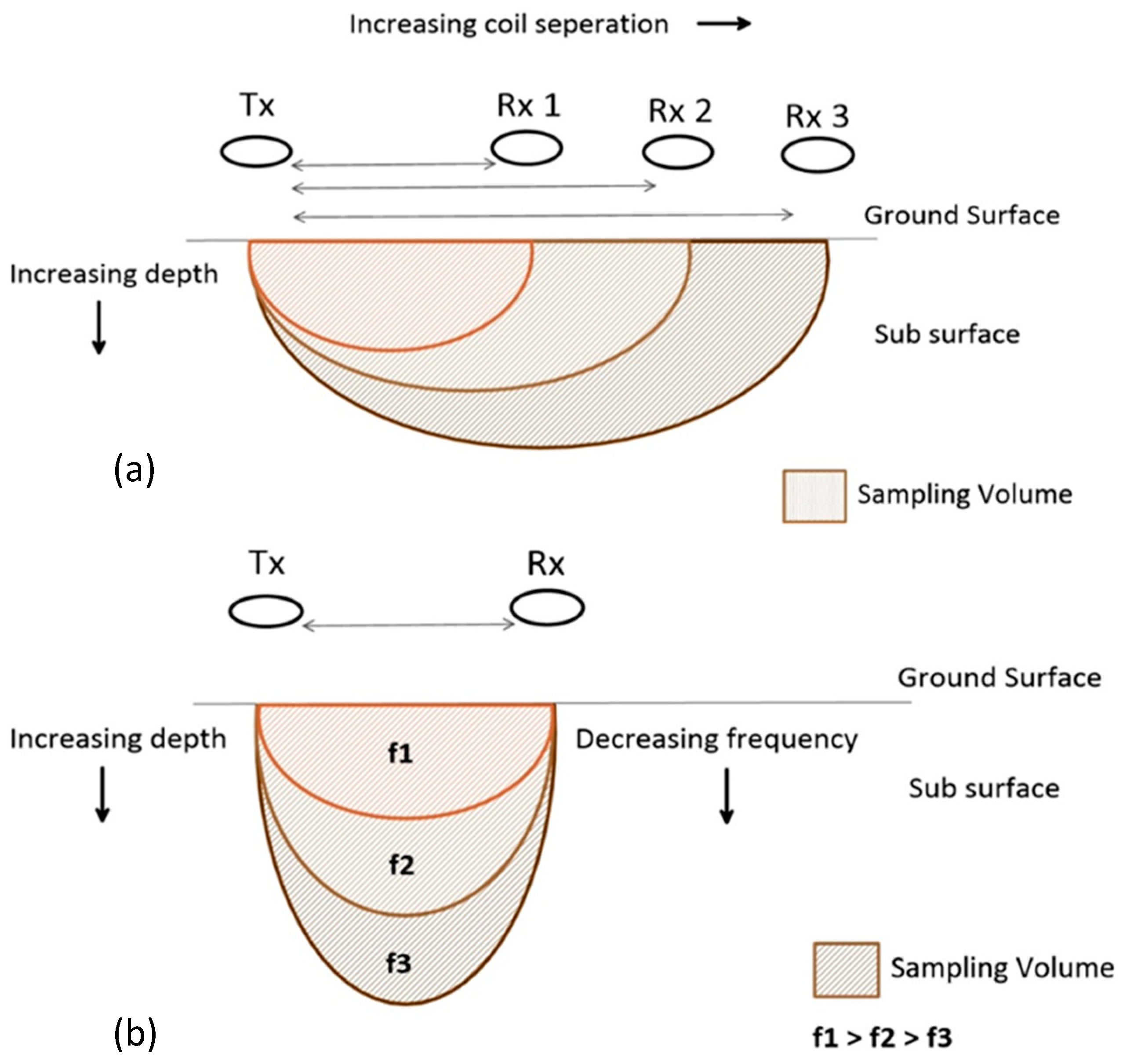
Multiple depth sensing/depth of penetrationsenses multiple depths with different frequencies and different waves (direct ground wave, reflected wave)
antennas should be changed to investigate deeper depths with lower resolution or shallow depths with higher resolution
senses different depths with different frequencies, inter-coil spacings, and coil orientation
senses different depths simultaneously, unlike GPR
Set up and operation may be challenging for non-technical individuals without advanced geophysics knowledge
newest technologies are making automated robotics to address this issue
relatively straightforward for non-technical individuals without advanced geophysical knowledge
Instrument costrelatively expensive compared to EMIrelatively affordable compared to GPR
Data processingrequires sophisticated data processing and interpretation skillsbasic data processing and interpretation are straightforward
Disclaimer/Publisher’s Note: The statements, opinions and data contained in all publications are solely those of the individual author(s) and contributor(s) and not of MDPI and/or the editor(s). MDPI and/or the editor(s) disclaim responsibility for any injury to people or property resulting from any ideas, methods, instructions or products referred to in the content.

