Technical Note

Uncertainty of Partial Dependence Relationship between Climate and Vegetation Growth Calculated by Machine Learning Models

1
College of Forestry, Precision Forestry Key Laboratory of Beijing, Beijing Forestry University, Beijing 100083, China
2
MOE Laboratory for Earth Surface Processes, College of Urban and Environmental Sciences, Peking University, Beijing 100871, China
3
Geography, Faculty of Environment Science and Economy, University of Exeter, Exeter EX4 4RJ, UK
4
Faculty of Agriculture, Food and Environment, The Hebrew University of Jerusalem, Rehovot 7610001, Israel
5
Key Laboratory of Ecosystem Network Observation and Modeling, Institute of Geographic Sciences and Natural Resources Research, Chinese Academy of Sciences, Beijing 100101, China
6
National Ecosystem Science Data Center, Beijing 100101, China
*
Author to whom correspondence should be addressed.
Remote Sens. 2023, 15(11), 2920; https://doi.org/10.3390/rs15112920
Submission received: 1 May 2023 / Revised: 27 May 2023 / Accepted: 31 May 2023 / Published: 3 June 2023
(This article belongs to the Special Issue Machine Learning in Global Change Ecology: Methods and Applications)

Abstract

:
As more machine learning and deep learning models are applied in studying the quantitative relationship between the climate and terrestrial vegetation growth, the uncertainty of these advanced models requires clarification. Partial dependence plots (PDPs) are one of the most widely used methods to estimate the marginal effect of independent variables on the predicted outcome of a machine learning model, and it is regarded as the main basis for conclusions in relevant research. As more controversies regarding the reliability of the results of the PDPs emerge, the uncertainty of the PDPs remains unclear. In this paper, we experiment with real, remote sensing data to systematically analyze the uncertainty of partial dependence relationships between four climate variables (temperature, rainfall, radiation, and windspeed) and vegetation growth, with one conventional linear model and six machine learning models. We tested the uncertainty of the PDP curves across different machine learning models from three aspects: variation, whole linear trends, and the trait of change points. Results show that the PDP of the dominant climate factor (mean air temperature) and vegetation growth parameter (indicated by the normalized difference vegetation index, NDVI) has the smallest relative variation and the whole linear trend of the PDP was comparatively stable across the different models. The mean relative variation of change points across the partial dependence curves of the non-dominant climate factors (i.e., radiation, windspeed, and rainfall) and vegetation growth ranged from 8.96% to 23.8%, respectively, which was much higher than those of the dominant climate factor and vegetation growth. Lastly, the model used for creating the PDP, rather than the relative importance of these climate factors, determines the fluctuation of the PDP output of these climate variables and vegetation growth. These findings have significant implications for using remote sensing data and machine learning models to investigate the quantitative relationships between the climate and terrestrial vegetation.

1. Introduction

Growth and functionality of terrestrial vegetation are highly affected by climate variables [1,2,3]. Quantifying the effects of the climate on terrestrial vegetation growth has been a hot topic in climate change research [4,5,6,7,8,9,10]. In the last two decades, remote sensing technology, machine learning, and deep learning algorithms have made it possible to elaborate the quantitative relationship between the climate and vegetation growth on a global scale [11,12,13]. However, uncertainties accompanied with the new models and technologies have also been perceived as one of the main challenges for understanding the relationship between the climate and terrestrial vegetation growth, as well as implementing climate mitigation action strategies [14,15].
Compared with the conventional statistical methods, machine learning and deep learning models estimate the nonlinear relationships between the climate and vegetation parameters that are not summarized by a small number of interpretable parameters. Instead, their model structures often contain huge numbers of parameters from which the quantitative relationship derives [16,17]. Despite the “black box” reputation of machine learning and deep learning models regarding interpretation, there are plenty of insights to be gained by investigating these models at different levels (e.g., interpretations at system, variable, and individual prediction levels, respectively) [18,19,20].
At the system level, the fitting performance of machine learning models is evaluated with metrics such as r2 (the proportion of the variance of the observed values explained by the predictions) or the root mean squared error (RMSE), which indicates how well the covariates can quantitatively explain the response variable based on the specified models. At the variable level, the variable importance can be assessed, i.e., examining the importance of the interactions between pairs of covariates and the functional responses of these covariates. The first step is to calculate the factor importance for the machine learning models [11,17,21,22]. Once the essential covariates have been identified based on the factor importance, it is useful to further investigate the variable level relationship between the covariate and the response. For example, the partial dependence plot (PDP) shows the marginal effect that the targeted features have on the predicted outcome of a machine learning model. PDPs are created by evaluating the mean response of the dependent variable to the change in the targeted covariate. It shows different patterns of quantitative relationship (linear, monotonic, or more complex) between the targeted covariate and the dependent variable [23,24]. For studies focusing on quantifying the impact of climate change on vegetation growth using machine learning models, PDPs are the main basis from which the core conclusions can be formulated [4,25,26,27].
However, while other uncertainties of using machine learning models in estimating quantitative impacts of climate on vegetation growth have been examined, the uncertainty associated with the partial dependence relationship has not been fully investigated. In this study, we tested the variation of the partial dependence relationship between the normalized difference vegetation index (NDVI) of the northern hemisphere deciduous broad-leaved forest and four influencing climatic factors (temperature, rainfall, radiation, and windspeed) across different machine learning and deep learning models, conducting a detailed analysis of the variation characteristics of the PDP by undertaking different statistical methods. This study is vital for understanding the uncertainties and assessing the accuracy behind the emerging “black box” models.

2. Method

Here we conducted an experiment to simulate a study calculating the partial dependence relationship between the climate parameters and vegetation growth based on remote sensing data and several machine learning models. NDVI was chosen as the proxy for vegetation growth, while the independent climate factors are annual mean temperature (referred to as temperature), annual rainfall (referred to as rainfall), shortwave radiation (referred to as radiation), and windspeed. Then, we imported seven statistical models (including six different machine learning and deep learning models, with a conventional multi-linear model as the comparison group) to calculate the partial dependence relationship between the four climate factors and NDVI (Table 1).
We selected deciduous broad-leaved forests in the northern hemisphere as our study region due to its relatively concentrated distribution range, with similar interactive mechanisms observed between the climate and local vegetation (Figure 1). The land cover data was based on the product MCD12C1 using annual data covering the period 2001–2016 [43]. We first upscaled the dataset from 0.05° to 0.5° of spatial resolution. For each 0.5° pixel, we assigned the land cover type for which the percentage was above 50% for all the subpixels. We extracted the pixels where the land cover type stayed constant over the study period (2001–2016).

2.1. Data Resources

2.1.1. MODIS NDVI

The dataset NDVI (MOD13C1, version 6.1, 2001–2016) was downloaded from the MODIS product website (https://lpdaac.usgs.gov/products/mod13c1v006/, accessed on 1 March 2022). The spatial resolution was 5 km and temporal interval was 16 days, respectively [44,45]. We resampled this dataset to the spatial resolution of 0.5° (in accordance with the meteorological dataset detailed in 2.1.2 below) and extracted the time series NDVI data in deciduous broad-leaved forests in the northern hemisphere, which acted as the dependent variable indicating vegetation growth.

2.1.2. WFDEI Meteorological Dataset

The European Union Water and Global Change project (http://www.eu-watch.org, accessed on 1 March 2022), provided a gridded European Union Water and Global Change-Forcing-Data-ERA-Interim (WFDEI) data product [46]. The WFDEI data product contains several kinds of meteorological variables with a spatial resolution of 0.5° and temporal resolution of 3 h (2001–2016). We resampled the original data to form meteorological data with a temporal resolution of 16 days, in accordance with the NDVI dataset (2.1.1). The independent meteorological variables influencing NDVI of vegetation included temperature, rainfall, radiation, and windspeed.
After unifying the spatio-temporal resolution for all remote sensing products, the PDP was calculated and developed based on the value of all NDVI pixels and four climate factors at the 16 days temporal scale.

2.2. Methods for Analysis

The partial dependence plot is a graphical representation of the marginal effect of a feature(s) on the predicted outcome of a machine learning model. It shows how the output variable changes when one or more features are changed. PDPs are useful for understanding the relationship between the output variable and the features in a machine learning model. The process of calculating and creating PDPs can be described as controlling the non-targeted features while shifting the targeted feature to quantitatively estimate the variation of the model output. We repeated the same step for each independent feature and created PDPs for the machine learning models, respectively.
The definition of partial dependence function for regression is:
f ^ S ( x S ) = E X C [ f ^ ( x S , X C ) ] = f ^ ( x S , X C )   d P ( X C )
where xS are the targeted feature(s) selected to create the PDP and XC are the other features impacting the result of the machine learning model f ^ . Namely, the feature xs is the independent variable for which we want to know the effect on model f predictions (dependent variable). Together, the feature vectors xS and XC combine the total feature space x (independent variable). The partial dependence function runs by marginalizing the machine learning model f output over the distribution of the features in XC. Therefore, this function shows the relationship between the features in xS that we are interested in and the result of the model prediction (dependent variable). By marginalizing over the other features, the above function only depends on features in xS.
Then the function of fS is calculated using Monte Carlo method:
f ^ S ( x S ) = 1 n i = 1 n f ^ ( x S , x C ( i ) )
Based on the above equation, for given value(s) of the features xS, the average marginal effect on the prediction is calculated. In this formula, x C ( i ) are the other feature values from the dataset for the other features excluding the selected target feature, and n is the number of instances in the dataset [47,48].
After producing PDPs for the seven statistical models, we analyzed the variation of the PDP curve from four perspectives:
(1) The overall variation of the curve shape for the PDP curves. We set different percentile intervals for calculating the variation of the response of the NDVI to the change of the climate factors across the different models used.
(2) The variation of the linear trend for PDP curves. First, we performed linear regression for each PDP based on the least squares principle:
y = a x + b
where y and x refer to the NDVI and each climate factor, respectively. The linear trend is the slope (a) of the fitting line, which demonstrates the macro influence (positive or negative, significant or not) of climate on NDVI in the PDP.
(3) Characteristics of the change points (which were evaluated by setting different threshold values for detecting one, two, or three change points, respectively) for each PDP, using MANOVA (multivariate analysis of variance) to test the influencing factors on the total number of change points in each PDP. Change points indicate abrupt variations within the PDP curves.
(4) Fluctuation of the PDP curves in the frequency domain based on the detrended Fourier decomposition, excluding the influence of the linear trend of the PDP. Fluctuations reveal the fast-varying parts in the PDP.
All steps were processed using relevant statistical packages (e.g., RegressionTree and newgrnn for building BRT and GRNN models, respectively) in Matlab 2021b.

3. Results

3.1. Overall Variation of the PDPs

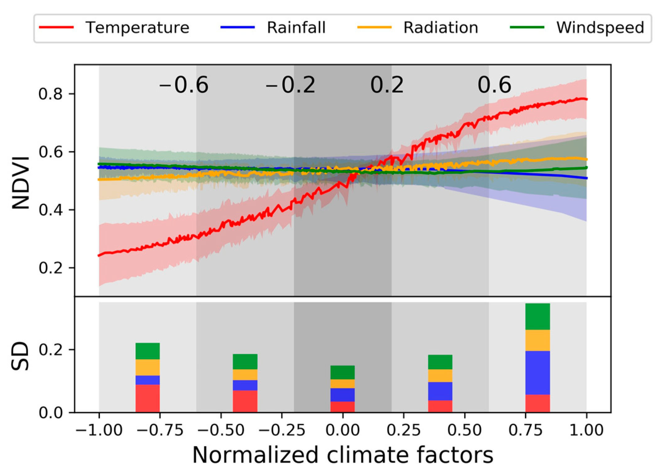
The PDP of each climate factor and NDVI have similar curve features among the seven statistical models (detailed in Supplementary Material). Among the four influencing climate factors, NDVI was found to have the most sensitivity to temperature change (Figure 2). The PDP of NDVI and temperature follows an approximately S-shaped curve. In contrast, NDVI has a varied response to changes in rainfall, radiation, and windspeed. The standard deviation (SD) of each curve (indicated by the shaded area around each line) increases towards both ends of the curve from the midrange values of the normalized climate factors. For example, the SD value is 0.149 in the midrange interval of [−0.2, 0.2] for the four curves combined, while the value in the interval of [0.2, 0.6] and [0.6, 1] is 0.183 and 0.346, respectively. This phenomenon shows that the difference in the PDP curve calculated by the different models is the smallest in the midrange of the climate factors. Considering the sensitivity of NDVI to temperature change, the corresponding relative variation is the smallest among all the climate factors.

3.2. Linear Trend of PDP

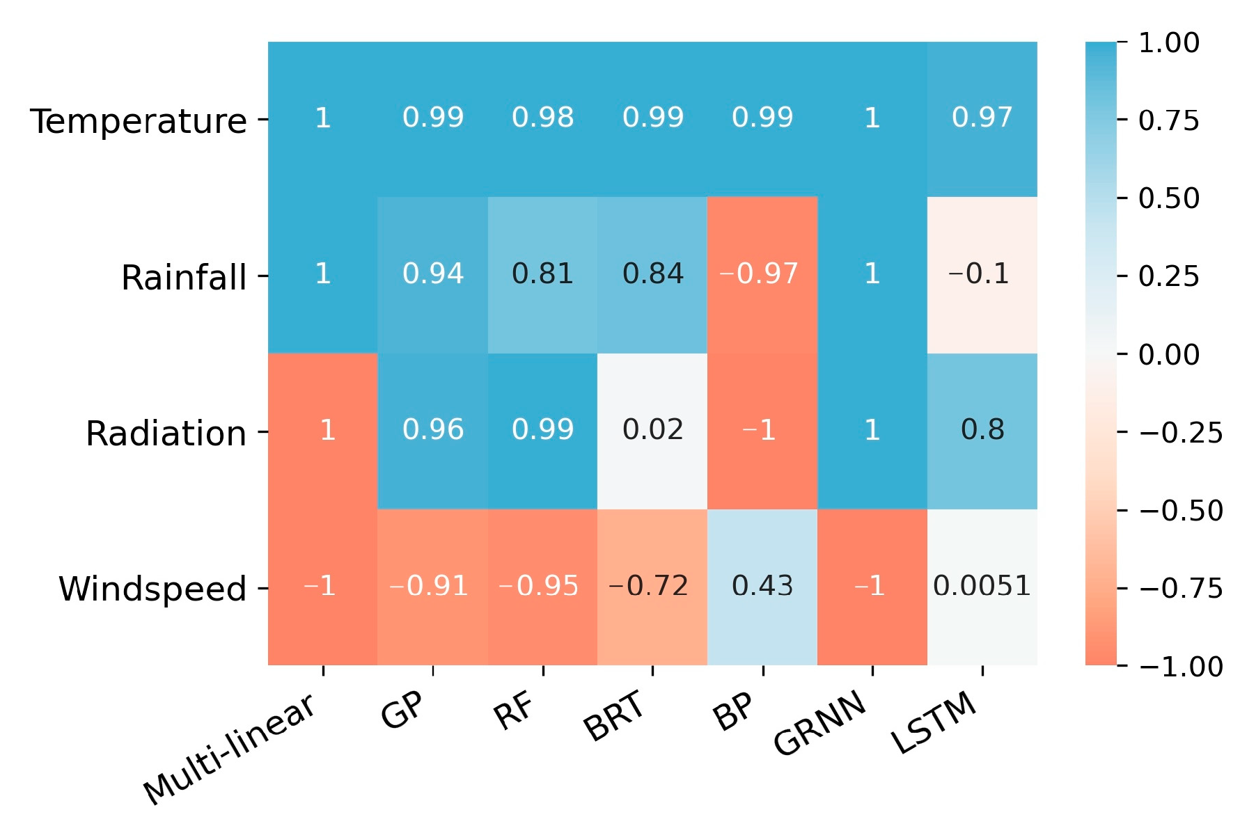
The similarity in the linear trend of PDP was calculated using different statistical models and varied among the different climate factors (Figure 3). The linear trend had a positive slope for the PDP of NDVI and temperature across all seven models. However, the linear trend for the PDP of NDVI and radiation was a significantly negative slope in the multi-linear and BP models, but positive in all the other models. With the exception of the climate factor of temperature, the other three influencing factors had this unconformity of positive or negative slopes of PDP across the different models.

3.3. Characteristics and Influencing Factors of Change Points

In the three scenarios for detecting the different numbers of change points for each PDP, the average relative variations of the four climate factors was 15.78%, 12.60%, and 10.73%, for one, two, and three change points, respectively (Table 2). Among the four climate factors, temperature had the smallest relative variation of 11.5%, 4.4%, and 5.0%, while rainfall was found to have the largest relative variation of 21.4%, 23.8%, and 19.8%, respectively.
Among the seven statistical models, the PDP calculated by the LSTM was found to have the most change points, with an average value of 240 (Table S1), followed by BRT and RF (with average values of 60 and 87, respectively). MANOVA analyzed the impact of the model and climate factor on the total number of change points for the PDPs, using every local maximum or minimum point in each PDP curve. The results indicated that the statistical model used has the most significant influence (p < 0.0001), and the climate factor is not the determinant (p > 0.1; Table 3).

3.4. Fluctuation of PDP in the Frequency Domain

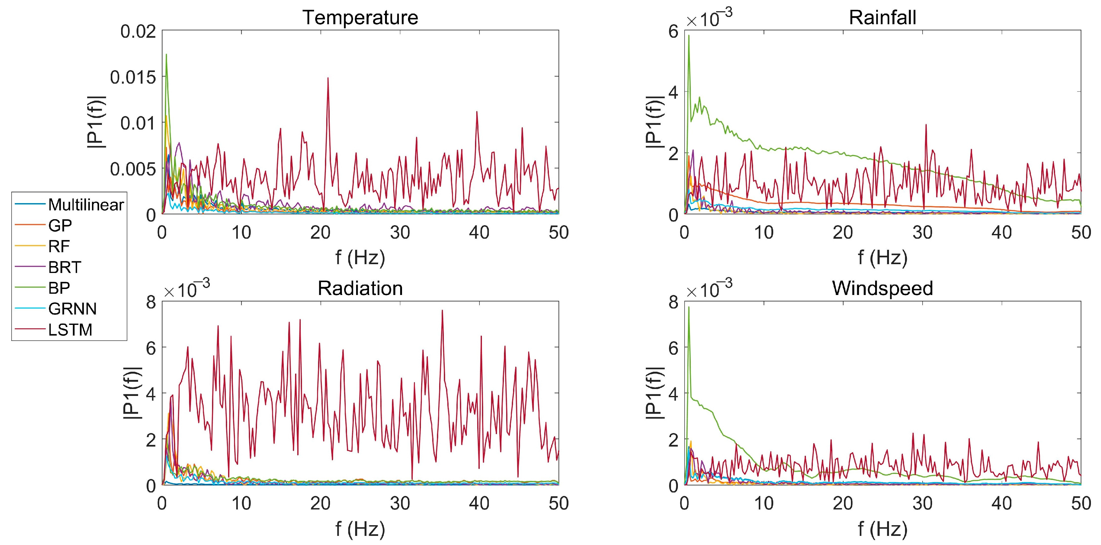
The results of the detrended Fourier decomposition demonstrates the fast-varying components and degree of detail of the PDP of the climate factors and NDVI. Among the seven statistical models, the PDP calculated by LSTM model for all four pairs of climate factors and NDVI had the highest value of P1 (red line in the four subplots; Figure 4) in both the medium and high frequency domains (higher than 10 Hz), indicating that the fluctuation of the curves is more evident than others. Compared with the different climate factors, the statistical model used was more dominant in determining the fluctuation traits of the PDPs. This phenomenon can also be seen in Supplementary Figure S1.

4. Discussion

The development of remote sensing (from the data resources perspective) and machine learning technology (from the methodology perspective) have greatly promoted this pursuit of better fitting ability and quantitative interpretation for environmental remote sensing research. While the uncertainty of interpretation for factor importance has been studied, our results showed that the uncertainty of machine learning interpretation at a more detailed level needs to be addressed as well. In our experiment, the determination coefficient of all seven models was over 0.8, thereby showing an ideal fitting accuracy (Table S2). However, the PDPs for the climate factors and NDVI revealed evident differences in terms of the curve shape, linear trend, change points, and fluctuation traits. Ignoring this uncertainty may induce significant divergence and therefore reduce the credibility of the associated conclusions.
Based on the results above, we present the recommended steps to be followed for controlling the uncertainty in calculating and creating PDPs between the environmental factors (e.g., climate variables) and vegetation parameters using machine learning models in future studies. Firstly, the whole fitting accuracy (indicated by RMSE and R2 and other alternative proxies) for the selected machine learning models needs to be evaluated. Once the fitting performance meets the requirement, the dominant and other important factors should then be identified for the second step. The index for this step can be chosen as either the Pearson’s correlation coefficient, partial correlation coefficient, or factor importance. In our experiment, the mean temperature was found to have the maximum Pearson’s correlation coefficient (0.87) with NDVI, after excluding the multicollinearity of climate factors (Figure S2, all the other Pearson’s correlation coefficients between the different climate factors and NDVI were less than 0.6). The dominance of temperature on vegetation growth in the study region was found to be in accordance with previous studies [49,50]. The last step is to rationally use PDPs for relative analysis and drawing conclusions. The more dominant the variable is, the more stable the resultant PDP of this factor (e.g., temperature) and the dependent factor (e.g., NDVI). For example, the PDPs of temperature and NDVI have the least relative variation, compared with the other three climate factors (rainfall, radiation, and windspeed). The response of NDVI to temperature change calculated by all seven models followed an S-shaped curve. In contrast, the PDP of the other three climate factors and NDVI had more uncertainty in the curve shape, with the average shape being relatively flat (Figure 2). Additionally, the linear trend of the PDPs of temperature and NDVI was more stable than other climate factors (Figure 3). This relative stability in the PDP of these dominant factors and NDVI was also shown in the change points of the curves (Table 2). This was due to the high sensitivity of NDVI to temperature variation, which was shown by the corresponding PDP with a clear curve structure and more variation tolerance. Additionally, when analyzing the details of the PDP curves, the uncertainty brought by different machine learning models cannot be neglected. For all pairs between the four climate factors and NDVI, the resultant PDP curve from the LSTM models were always found to have the most change points, while the curves created by BP and GRNN were much smoother (with no change points of PDP detected, Table S1). This phenomenon was mainly caused by the specific structure of each machine learning model [51]. At last, PDP curves for the different machine learning models showed less variation in the midrange of independent variables (Figure 2). This is because the training dataset for machine learning models tends to be larger in this data region than those distributed at both ends. Thus, the fitting accuracy was higher and more stable, which further influenced the traits of the PDP.
Following the invention of new machine learning models, the corresponding methods for interpreting the quantitative relationships inside each model were raised successively. For artificial neural networks, several alternative methods can be selected to calculate the relative importance of the included independent factors in each network. Previous studies showed that both the value of relative importance and the rank of independent variables based on their impact differed greatly among the methods [21,22]. Recently, more novel methods were employed in research analyzing the quantitative relationship in machine learning models from different perspectives. For example, some model-diagnostic, local explanation approaches were designed to explain any given machine learning models displaying “black box” characteristics [52,53,54,55,56,57,58]. These methods can explain the individual predictions of any classifier in an interpretable manner by learning an interpretable model (e.g., linear model) locally around each prediction. However, few studies have yet mentioned the potential uncertainty they may have on the result of interpretation. The results and analyzes in this study imply that the exclusion of this uncertainty brought by the machine learning methods may reduce the credibility of the associated conclusions. In addition to uncertainty brought by data resources and model parameters, we suggest that the variation across the different machine learning and deep learning models should be highly emphasized.
Several other factors which were not evaluated in this study may also impact the variation of the PDP in machine learning models, for example, the hyper-parameter settings and training mode of each model. Hyper-parameters are parameters that are not learned by the model during training but are set prior to training [59,60]. In the context of artificial neural networks, hyperparameters are used to control the architecture of the network and the learning process. Examples of hyperparameters in neural networks include the learning rate, number of hidden layers, number of neurons in each hidden layer, activation function, regularization parameter etc. More systematic studies may therefore be considered in subsequent research.
In the future, when applying machine learning and deep learning methods in environmental remote sensing research, researchers are strongly recommended to evaluate the uncertainty of both the models and the method used. This evaluation of uncertainty should include more detailed examinations of the quantitative relationships calculated by the machine learning and deep learning models (e.g., using the Monte Carlo method to estimate the uncertainty across models in different data intervals). Only in this way can the research conclusions be robust and more significant for reference.

5. Conclusions

Driven by remote sensing technology and machine learning models, investigations into the quantitative relationships between the climate and terrestrial vegetation in global change studies have emerged in an unprecedented pattern. As an essential basis for drawing relative conclusions, the stability of the PDP has a direct impact on the credibility of the research. Overall, the relative importance of the influencing factors, the selected model structures, and the specific interval in the plot are the three key elements affecting the uncertainty of the PDP curve, which should be fully evaluated. We also provided several suggestions for controlling the uncertainty in calculating PDP, including considering the performance of the machine learning model, the selected index, the factor impact of each influencing factor and details of PDP interpretation. As large numbers of new algorithm structures and relationship interpretation methods have been proposed, reasonable exploration of the uncertainty of the different methods used and the analysis of its influencing factors are indispensable for future studies.

Supplementary Materials

The following supporting information can be downloaded at: https://www.mdpi.com/article/10.3390/rs15112920/s1, Figure S1. Partial dependence plots of climate factors and NDVI calculated by different statistical models. Figure S2. Cross correlation coefficient for each pair of climate factors and NDVI (T is mean air temperature). Table S1. Total number of change point for each partial dependence plot. Table S2. Mean determination coefficient of each statistical model.

Author Contributions

Methodology, B.L. and J.D.; Validation, B.L. and C.X.; Investigation, B.L. and Z.W.; Writing—original draft, B.L.; Writing—review & editing, H.L., E.L.C. and L.W.; Visualization, L.S.; Supervision, J.W.; Project administration, H.L.; Funding acquisition, H.L. All authors have read and agreed to the published version of the manuscript.

Funding

Grants the paper has been funded by the National Key Research and Development Program (2022YFF0801803) and the Fundamental Research Funds for the Central Universities (BLX202105 and BLX202107).

Conflicts of Interest

The authors declare that they have no known competing financial interest or personal relationships that could have appeared to influence the work reported in this paper.

References

  1. Ma, X.; Huete, A.; Moran, S.; Ponce-Campos, G.; Eamus, D. Abrupt shifts in phenology and vegetation productivity under climate extremes. J. Geophys. Res. Biogeosci. 2015, 120, 2036–2052. [Google Scholar] [CrossRef]
  2. Piao, S.; Wang, X.; Park, T.; Chen, C.; Lian, X.; He, Y.; Bjerke, J.W.; Chen, A.; Ciais, P.; Tømmervik, H. Characteristics, drivers and feedbacks of global greening. Nat. Rev. Earth Environ. 2020, 1, 14–27. [Google Scholar] [CrossRef] [Green Version]
  3. Liu, Y.; Kumar, M.; Katul, G.G.; Porporato, A. Reduced resilience as an early warning signal of forest mortality. Nat. Clim. Chang. 2019, 9, 880–885. [Google Scholar] [CrossRef]
  4. Li, Y.; Zhang, W.; Schwalm, C.R.; Gentine, P.; Smith, W.K.; Ciais, P.; Kimball, J.S.; Gazol, A.; Kannenberg, S.A.; Chen, A. Widespread spring phenology effects on drought recovery of Northern Hemisphere ecosystems. Nat. Clim. Chang. 2023, 13, 182–188. [Google Scholar] [CrossRef]
  5. Zhao, Q.; Zhu, Z.; Zeng, H.; Myneni, R.B.; Zhang, Y.; Peñuelas, J.; Piao, S. Seasonal peak photosynthesis is hindered by late canopy development in northern ecosystems. Nat. Plants 2022, 8, 1484–1492. [Google Scholar] [CrossRef]
  6. Chen, L.; Hänninen, H.; Rossi, S.; Smith, N.G.; Pau, S.; Liu, Z.; Feng, G.; Gao, J.; Liu, J. Leaf senescence exhibits stronger climatic responses during warm than during cold autumns. Nat. Clim. Chang. 2020, 10, 777–780. [Google Scholar] [CrossRef]
  7. Wu, C.; Wang, J.; Ciais, P.; Peñuelas, J.; Zhang, X.; Sonnentag, O.; Tian, F.; Wang, X.; Wang, H.; Liu, R. Widespread decline in winds delayed autumn foliar senescence over high latitudes. Proc. Natl. Acad. Sci. USA 2021, 118, e2015821118. [Google Scholar] [CrossRef]
  8. Moles, A.T.; Perkins, S.E.; Laffan, S.W.; Flores-Moreno, H.; Awasthy, M.; Tindall, M.L.; Sack, L.; Pitman, A.; Kattge, J.; Aarssen, L.W. Which is a better predictor of plant traits: Temperature or precipitation? J. Veg. Sci. 2014, 25, 1167–1180. [Google Scholar] [CrossRef]
  9. Collalti, A.; Ibrom, A.; Stockmarr, A.; Cescatti, A.; Alkama, R.; Fernández-Martínez, M.; Matteucci, G.; Sitch, S.; Friedlingstein, P.; Ciais, P.; et al. Forest production efficiency increases with growth temperature. Nat. Commun. 2020, 11, 5322. [Google Scholar] [CrossRef]
  10. Zellweger, F.; De Frenne, P.; Lenoir, J.; Vangansbeke, P.; Verheyen, K.; Bernhardt-Römermann, M.; Baeten, L.; Hédl, R.; Berki, I.; Brunet, J.; et al. Forest microclimate dynamics drive plant responses to warming. Science 2020, 368, 772–775. [Google Scholar] [CrossRef]
  11. Murray, K.; Conner, M.M. Methods to quantify variable importance: Implications for the analysis of noisy ecological data. Ecology 2009, 90, 348–355. [Google Scholar] [CrossRef] [Green Version]
  12. Meyer, H.; Pebesma, E. Machine learning-based global maps of ecological variables and the challenge of assessing them. Nat. Commun. 2022, 13, 1–4. [Google Scholar] [CrossRef] [PubMed]
  13. Li, X.; Piao, S.; Wang, K.; Wang, X.; Wang, T.; Ciais, P.; Chen, A.; Lian, X.; Peng, S.; Peñuelas, J. Temporal trade-off between gymnosperm resistance and resilience increases forest sensitivity to extreme drought. Nat. Ecol. Evol. 2020, 4, 1075–1083. [Google Scholar] [CrossRef]
  14. Reichstein, M.; Camps-Valls, G.; Stevens, B.; Jung, M.; Denzler, J.; Carvalhais, N.; Prabhat. Deep learning and process understanding for data-driven Earth system science. Nature 2019, 566, 195–204. [Google Scholar] [CrossRef] [PubMed]
  15. Yuan, Q.; Shen, H.; Li, T.; Li, Z.; Li, S.; Jiang, Y.; Xu, H.; Tan, W.; Yang, Q.; Wang, J.; et al. Deep learning in environmental remote sensing: Achievements and challenges. Remote Sens. Environ. 2020, 241, 111716. [Google Scholar] [CrossRef]
  16. Fassnacht, F.E.; Neumann, C.; Förster, M.; Buddenbaum, H.; Ghosh, A.; Clasen, A.; Joshi, P.K.; Koch, B. Comparison of feature reduction algorithms for classifying tree species with hyperspectral data on three central European test sites. IEEE J. Sel. Top. Appl. Earth Obs. Remote Sens. 2014, 7, 2547–2561. [Google Scholar] [CrossRef]
  17. Kosicki, J.Z. Generalised Additive Models and Random Forest Approach as effective methods for predictive species density and functional species richness. Environ. Ecol. Stat. 2020, 27, 273–292. [Google Scholar] [CrossRef]
  18. Lucas, T.C.D. A translucent box: Interpretable machine learning in ecology. Ecol. Monogr. 2020, 90, e01422. [Google Scholar] [CrossRef]
  19. Lipton, Z.C. The Mythos of Model Interpretability: In machine learning, the concept of interpretability is both important and slippery. Queue 2018, 16, 31–57. [Google Scholar] [CrossRef]
  20. Wu, M.; Hughes, M.; Parbhoo, S.; Zazzi, M.; Roth, V.; Doshi-Velez, F. Beyond sparsity: Tree regularization of deep models for interpretability. In Proceedings of the Proceedings of the AAAI Conference on Artificial Intelligence, New Orleans, LA, USA, 2–7 February 2018. [Google Scholar]
  21. Gevrey, M.; Dimopoulos, I.; Lek, S. Review and comparison of methods to study the contribution of variables in artificial neural network models. Ecol. Model. 2003, 160, 249–264. [Google Scholar] [CrossRef]
  22. Olden, J.D.; Joy, M.K.; Death, R.G. An accurate comparison of methods for quantifying variable importance in artificial neural networks using simulated data. Ecol. Model. 2004, 178, 389–397. [Google Scholar] [CrossRef]
  23. Greenwell, B.M. pdp: An R Package for constructing partial dependence plots. R J. 2017, 9, 421. [Google Scholar] [CrossRef] [Green Version]
  24. Shi, H.; Yang, N.; Yang, X.; Tang, H. Clarifying Relationship between PM2. 5 Concentrations and Spatiotemporal Predictors Using Multi-Way Partial Dependence Plots. Remote Sens. 2023, 15, 358. [Google Scholar] [CrossRef]
  25. Yao, Y.; Liu, Y.; Zhou, S.; Song, J.; Fu, B. Soil moisture determines the recovery time of ecosystems from drought. Glob. Chang. Biol. 2023, 1–13. [Google Scholar] [CrossRef] [PubMed]
  26. Campbell, T.K.F.; Lantz, T.C.; Fraser, R.H.; Hogan, D. High Arctic vegetation change mediated by hydrological conditions. Ecosyst. 2021, 24, 106–121. [Google Scholar] [CrossRef]
  27. Zhang, Y.; Keenan, T.F.; Zhou, S. Exacerbated drought impacts on global ecosystems due to structural overshoot. Nat. Ecol. Evol. 2021, 5, 1490–1498. [Google Scholar] [CrossRef]
  28. Wu, X.; Li, X.; Chen, Y.; Bai, Y.; Tong, Y.; Wang, P.; Liu, H.; Wang, M.; Shi, F.; Zhang, C. Atmospheric water demand dominates daily variations in water use efficiency in alpine meadows, northeastern Tibetan Plateau. J. Geophys. Res. Biogeosci. 2019, 124, 2174–2185. [Google Scholar] [CrossRef]
  29. Schaffers, A.P. Soil, biomass, and management of semi-natural vegetation–Part II. Factors controlling species diversity. Plant Ecol. 2002, 158, 247–268. [Google Scholar] [CrossRef]
  30. Ingram, M.; Vukcevic, D.; Golding, N. Multi-output Gaussian processes for species distribution modelling. Methods Ecol. Evol. 2020, 11, 1587–1598. [Google Scholar] [CrossRef]
  31. Peters, J.; Verhoest, N.E.C.; Samson, R.; Boeckx, P.; De Baets, B. Wetland vegetation distribution modelling for the identification of constraining environmental variables. Landsc. Ecol. 2008, 23, 1049–1065. [Google Scholar] [CrossRef]
  32. Prasad, A.M.; Iverson, L.R.; Liaw, A. Newer classification and regression tree techniques: Bagging and random forests for ecological prediction. Ecosystems 2006, 9, 181–199. [Google Scholar] [CrossRef]
  33. Oppel, S.; Strobl, C.; Huettmann, F. Alternative Methods to Quantify Variable Importance in Ecology; University of Munich: Munich, Germany, 2009. [Google Scholar]
  34. Vidal-Macua, J.J.; Nicolau, J.M.; Vicente, E.; Moreno-de Las Heras, M. Assessing vegetation recovery in reclaimed opencast mines of the Teruel coalfield (Spain) using Landsat time series and boosted regression trees. Sci. Total Environ. 2020, 717, 137250. [Google Scholar] [CrossRef] [PubMed]
  35. Zhi, J.; Zhou, Z.; Cao, X. Exploring the determinants and distribution patterns of soil mattic horizon thickness in a typical alpine environment using boosted regression trees. Ecol. Indic. 2021, 133, 108373. [Google Scholar] [CrossRef]
  36. Li, M.-Y.; Lai, X.-J. Evaluation on ecological security of urban land based on BP neural network-a case study of Guangzhou. Econ. Geogr. 2011, 31, 289–293. [Google Scholar]
  37. Xu, B.; Zhang, H.; Wang, Z.; Wang, H.; Zhang, Y. Model and algorithm of BP neural network based on expanded multichain quantum optimization. Math. Probl. Eng. 2015, 2015, 362150. [Google Scholar] [CrossRef] [Green Version]
  38. Li, J.; Cheng, J.-h.; Shi, J.-y.; Huang, F. Brief introduction of back propagation (BP) neural network algorithm and its improvement. In Advances in Computer Science and Information Engineering; Springer: Berlin/Heidelberg, Germany, 2012; pp. 553–558. [Google Scholar]
  39. Jia, K.; Liang, S.; Liu, S.; Li, Y.; Xiao, Z.; Yao, Y.; Jiang, B.; Zhao, X.; Wang, X.; Xu, S. Global land surface fractional vegetation cover estimation using general regression neural networks from MODIS surface reflectance. IEEE Trans. Geosci. Remote Sens. 2015, 53, 4787–4796. [Google Scholar] [CrossRef]
  40. Specht, D.F. A general regression neural network. IEEE Trans. Neural Netw. 1991, 2, 568–576. [Google Scholar] [CrossRef] [Green Version]
  41. Chen, Z.; Liu, H.; Xu, C.; Wu, X.; Liang, B.; Cao, J.; Chen, D. Modeling vegetation greenness and its climate sensitivity with deep-learning technology. Ecol. Evol. 2021, 11, 7335–7345. [Google Scholar] [CrossRef]
  42. Chen, Z.-T.; Liu, H.-Y.; Xu, C.-Y.; Wu, X.-C.; Liang, B.-Y.; Cao, J.; Chen, D. Deep learning projects future warming-induced vegetation growth changes under SSP scenarios. Adv. Clim. Chang. Res. 2022, 13, 251–257. [Google Scholar] [CrossRef]
  43. Sulla-Menashe, D.; Friedl, M.A. User Guide to Collection 6 MODIS Land Cover (MCD12Q1 and MCD12C1) Product; USGS: Rest, VA, USA, 2018. [Google Scholar]
  44. Didan, K. MOD13C1 MODIS/Terra Vegetation Indices 16-Day L3 Global 0.05 Deg CMG V006 [Dataset]. In NASA EOSDIS Land Process; DAAC: Greenbelt, MD, USA, 2015. [Google Scholar]
  45. Guo, X.; Zhang, H.; Wu, Z.; Zhao, J.; Zhang, Z. Comparison and evaluation of annual NDVI time series in China derived from the NOAA AVHRR LTDR and Terra MODIS MOD13C1 products. Sensors 2017, 17, 1298. [Google Scholar] [CrossRef] [Green Version]
  46. Weedon, G.P.; Balsamo, G.; Bellouin, N.; Gomes, S.; Best, M.J.; Viterbo, P. The WFDEI meteorological forcing data set: WATCH Forcing Data methodology applied to ERA-Interim reanalysis data. Water Resour. Res. 2014, 50, 7505–7514. [Google Scholar] [CrossRef] [Green Version]
  47. Molnar, C.; Freiesleben, T.; König, G.; Casalicchio, G.; Wright, M.N.; Bischl, B. Relating the partial dependence plot and permutation feature importance to the data generating process. arXiv 2021, arXiv:2109.01433. [Google Scholar]
  48. Moosbauer, J.; Herbinger, J.; Casalicchio, G.; Lindauer, M.; Bischl, B. Explaining hyperparameter optimization via partial dependence plots. Adv. Neural Inf. Process Syst. 2021, 34, 2280–2291. [Google Scholar]
  49. Hiura, T.; Go, S.; Iijima, H. Long-term forest dynamics in response to climate change in northern mixed forests in Japan: A 38-year individual-based approach. For. Ecol. Manag. 2019, 449, 117469. [Google Scholar] [CrossRef]
  50. Jin, G.; Liu, D. Mid-Holocene climate change in North China, and the effect on cultural development. Chin. Sci. Bull. 2002, 47, 408–413. [Google Scholar] [CrossRef]
  51. Pichler, M.; Boreux, V.; Klein, A.M.; Schleuning, M.; Hartig, F. Machine learning algorithms to infer trait-matching and predict species interactions in ecological networks. Methods Ecol. Evol. 2020, 11, 281–293. [Google Scholar] [CrossRef] [Green Version]
  52. Ryo, M.; Angelov, B.; Mammola, S.; Kass, J.M.; Benito, B.M.; Hartig, F. Explainable artificial intelligence enhances the ecological interpretability of black-box species distribution models. Ecography 2021, 44, 199–205. [Google Scholar] [CrossRef]
  53. Visani, G.; Bagli, E.; Chesani, F.; Poluzzi, A.; Capuzzo, D. Statistical stability indices for LIME: Obtaining reliable explanations for machine learning models. J. Oper. Res. Soc. 2022, 73, 91–101. [Google Scholar] [CrossRef]
  54. Bowen, D.; Ungar, L. Generalized SHAP: Generating multiple types of explanations in machine learning. arXiv 2020, arXiv:2006.07155. [Google Scholar]
  55. Mangalathu, S.; Hwang, S.-H.; Jeon, J.-S. Failure mode and effects analysis of RC members based on machine-learning-based SHapley Additive exPlanations (SHAP) approach. Eng. Struct. 2020, 219, 110927. [Google Scholar] [CrossRef]
  56. Maynard, D.S.; Bialic-Murphy, L.; Zohner, C.M.; Averill, C.; van den Hoogen, J.; Ma, H.; Mo, L.; Smith, G.R.; Acosta, A.T.R.; Aubin, I.; et al. Global relationships in tree functional traits. Nat. Commun. 2022, 13, 3185. [Google Scholar] [CrossRef]
  57. Bellot, S.; Lu, Y.; Antonelli, A.; Baker, W.J.; Dransfield, J.; Forest, F.; Kissling, W.D.; Leitch, I.J.; Nic Lughadha, E.; Ondo, I.; et al. The likely extinction of hundreds of palm species threatens their contributions to people and ecosystems. Nat. Ecol. Evol. 2022, 6, 1710–1722. [Google Scholar] [CrossRef] [PubMed]
  58. Webb, E.E.; Liljedahl, A.K.; Cordeiro, J.A.; Loranty, M.M.; Witharana, C.; Lichstein, J.W. Permafrost thaw drives surface water decline across lake-rich regions of the Arctic. Nat. Clim. Chang. 2022, 12, 841–846. [Google Scholar] [CrossRef]
  59. Hamida, S.; El Gannour, O.; Cherradi, B.; Ouajji, H.; Raihani, A. Optimization of machine learning algorithms hyper-parameters for improving the prediction of patients infected with COVID-19. In Proceedings of the 2020 IEEE 2nd International Conference on Electronics, Control, Optimization and Computer Science (Icecocs), Kenitra, Morocco, 2–3 December 2020; pp. 1–6. [Google Scholar]
  60. Subramanian, M.; Shanmugavadivel, K.; Nandhini, P. On fine-tuning deep learning models using transfer learning and hyper-parameters optimization for disease identification in maize leaves. Neural Comput. Appl. 2022, 34, 13951–13968. [Google Scholar] [CrossRef]
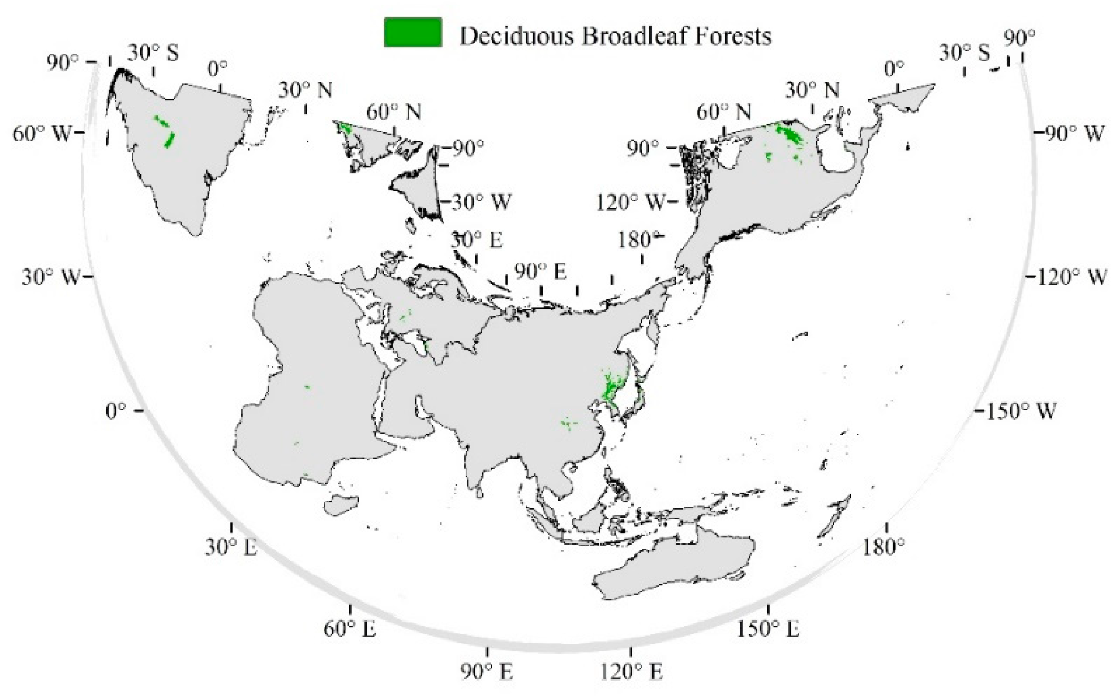
Figure 1. Distribution of constant deciduous broad-leaved forests (totaling 374 pixels in the northern hemisphere).
Remotesensing 15 02920 g001
Figure 2. PDP of four climate factors and NDVI (SD denotes standard deviation; solid line denotes the average PDP curve of NDVI and four climate factors calculated by the seven different models; shaded area around each solid line indicates the SD of PDP among the seven statistical models; and the value of the normalized climate factors was divided into five equal intervals, for which the percentiles were annotated and the SD of PDP in each interval were calculated, respectively).
Remotesensing 15 02920 g002
Figure 3. The linear trend of PDP curves of four climate factors and NDVI calculated with different models.
Remotesensing 15 02920 g003
Figure 4. Single-sided amplitude spectrum (P1) of the PDP in different frequency domains (f).
Remotesensing 15 02920 g004
Table 1. The statistical models utilized for calculating the partial dependence relationships.
CategoryModel NameGeneral EquationKey ParameterizationReference
Linear ModelMultivariate linear model y = a x 1 + b x 2 + c x 3 + + d -[6,28,29]
Non-parametric modelGaussian process model (GP) y = f ( X , ω ) ,   f g p ( μ , κ θ ) Default kernel function with parameters[30]
Regression tree modelsRandom forest (RF)-A total of 200 trees; minimum number of observations per tree leaf is 5[31,32,33]
Boosted regression tree (BRT)-Minimum number of observations per tree leaf is 5; learning rate is 0.01[34,35]
Artificial neural network modelsBack propagation (BP) neural network-Single hidden layer with 10 neurons; learning rate is 0.01[36,37,38]
General regression neural network (GRNN)-Spread of radial basis functions is 1[39,40]
Long short-term memory (LSTM) neural network-One LSTM layer with 500 hidden units and one fully connected layer; learning rate is 0.008[41,42]
Table 2. The statistical analysis of change points in the PDP of four climate factors and NDVI (relative variation is the value of mean deviation divided by the total interval length of normalized climate factor values).
Independent Factor of PDP
Maximum Number of Change PointsModelsTemperatureRainfallRadiationWindspeed
1Multi-linear0.58−0.39−0.340.39
GP0.260.140.530.05
RF0.31−0.84−0.21−0.41
BRT0.50−0.650.28-
BP−0.020.42-0.35
GRNN0.58−0.21−0.280.38
LSTM0.03−0.67−0.130.02
Mean deviation0.230.430.320.29
Mean relative variation11.5%21.4%15.9%14.3%
2Multi-linear[−0.25, 0.61][−0.61, 0.05]−0.340.39
GP[−0.47, 0.58][0.02, 0.90][−0.20, 0.46][−0.11, 0.25]
RF[−0.32, 0.56][−0.93, −0.83][−0.60, −0.22][−0.39, 0.07]
BRT[−0.21, 0.56][−0.91, −0.65][−0.42, 0.28][−0.32, −0.04]
BP[−0.26, 0.37][−0.64, 0.90][−0.28, 0.75][−0.01, 0.52]
GRNN[−0.25, 0.61][−0.59, 0.09][−0.44, 0.02][0.18, 0.53]
LSTM[−0.21, 0.69][−0.59, −0.58]−0.13[−0.08, 0.07]
Mean deviation0.090.480.24 0.21
Mean relative deviation4.4%23.8%11.9%10.3%
3Multi-linear[−0.25, 0.61][−0.63, −0.10, 0.90][−0.44, 0.02, 0.75][−0.68, 0.13, 0.52]
GP[−0.46, −0.02, 0.61][−0.88, 0.02, 0.90][−0.25, 0.40, 0.75][−0.23, 0.09, 0.42]
RF[−0.26, 0.29, 0.63][−0.93, −0.83, −0.65][−0.60, −0.22, 0.52][−0.45, −0.32, 0.07]
BRT[−0.54, −0.16, 0.56][−0.91, −0.65, −0.39][−0.42, 0.20 ,0.42][−0.32, −0.05, 0.47]
BP[−0.39, −0.02, 0.47][−0.72, 0.05, 0.90][−0.44, 0.06, 0.75][−0.19, 0.21, 0.54]
GRNN[−0.42, −0.02, 0.63][−0.63, −0.07, 0.90][−0.44, 0.02, 0.75][−0.68, 0.13, 0.52]
LSTM[−0.21, 0.69][−0.97, −0.59, −0.58][−0.22, 0.07, 0.16][−0.11, −0.08, 0.07]
Mean deviation0.100.400.170.19
Mean relative variation5.0%19.8%8.5%9.6%
Table 3. The result of MANOVA analysis on the total number of change points for the PDP curves.
Sum_sqdfFp
C(Factor, Sum)51.5730.240.87
C(Model, Sum)186,817.216427.850.00
Residual1309.9318
Disclaimer/Publisher’s Note: The statements, opinions and data contained in all publications are solely those of the individual author(s) and contributor(s) and not of MDPI and/or the editor(s). MDPI and/or the editor(s) disclaim responsibility for any injury to people or property resulting from any ideas, methods, instructions or products referred to in the content.