Estimating Crown Biomass in a Multilayered Fir Forest Using Airborne LiDAR Data

Abstract

The estimation of individual biomass components within tree crowns, such as dead branches (DB), needles (NB), and branch biomass (BB), has received limited attention in the scientific literature despite their significant contribution to forest biomass. This study aimed to assess the potential of multispectral LiDAR data for estimating these biomass components in a multi-layered Abies borissi-regis forest. Destructive (i.e., 13) and non-destructive (i.e., 156) field measurements were collected from Abies borisii-regis trees to develop allometric equations for each crown biomass component and enrich the reference data with the non-destructively sampled trees. A set of machine learning regression algorithms, including random forest (RF), support vector regression (SVR) and Gaussian process (GP), were tested for individual-tree-level DB, NB and BB estimation using LiDAR-derived height and intensity metrics for different spectral channels (i.e., green, NIR and merged) as predictors. The results demonstrated that the RF algorithm achieved the best overall predictive performance for DB (RMSE% = 17.45% and R² = 0.89), NB (RMSE% = 17.31% and R² = 0.93) and BB (RMSE% = 24.09% and R² = 0.85) using the green LiDAR channel. This study showed that the tested algorithms, particularly when utilizing the green channel, accurately estimated the crown biomass components of conifer trees, specifically fir. Overall, LiDAR data can provide accurate estimates of crown biomass in coniferous forests, and further exploration of this method’s applicability in diverse forest structures and biomes is warranted.

1. Introduction

Forests are considered among the most important carbon sinks since they are responsible for storing approximately 80% of all terrestrial carbon. Precise measurement and quantification of forest biomass and carbon are essential to mitigate climate change and optimize forest management strategies at global and regional scales [1]. Forest biomass includes both the above- (AGB) and below-ground biomass. The AGB can be defined as the sum of all living biomass components standing above the soil level (e.g., stem, leaves, needles, branches, bark), expressed as the mass of an individual tree or unit area [2,3,4]. The crown and more specifically, foliage is directly related to the primary production, photosynthesis, nutrient cycling, light transmission and understory vegetation, affecting tree growth and natural regeneration [5]. In addition, living and dead branches play significant roles in forest biomass dynamics as they constitute the majority of the logging residues [6] and have the highest carbon content among the tree components [7].

Conventional methods for AGB estimation require destructive sampling, which provides accurate and precise biomass estimation. However, it is time-consuming, laborious and costly [8]. Therefore, allometric equations are most commonly used for AGB estimation. In fact, these equations constitute regression models that can predict either the total biomass or the biomass of tree components as a function of morphometric measurements (e.g., DBH, tree height) [9,10].

Remote sensing techniques have been widely used to estimate forest biomass and other forest inventory attributes, due to their ability to provide low-cost, accurate and timely results over large and impassable areas [11,12]. Various remote sensing data have been tested for forest biomass and carbon quantification, such as optical (e.g., multi- and hyperspectral) [13,14,15,16], synthetic aperture radar (SAR) [17,18,19], light detection and ranging (LiDAR) [20,21,22,23,24], and integrations between them [25,26,27,28,29]. Multispectral and SAR image analyse are the most common approaches for large-scale biomass estimation. However, signal saturation is the main limitation for both of them, especially over forested areas with complex topographies [12,30]. Unlike optical sensors, LiDAR signals can penetrate through the forest canopy, providing valuable vertical information about the forest structure [31]. As a result, LiDAR data are less impacted by the shadow and saturation effects [32], delivering reliable forest biomass estimations over different biomes [33].

The potential of LiDAR data in the estimation of various forest characteristics, such as stem and components attributes [1,34,35,36], crown base height [37,38,39,40], leaf area index [41,42,43,44], biomass [1,20,39,45,46] and carbon [47,48,49], has been extensively explored using plot- and tree-based approaches. The first approach includes the implementation of height-derived and other LiDAR-related metrics to predict forest characteristics at the plot or stand level while the second approach provides detailed forest information at different scales [50]. According to [49], the plot-level approach provides more accurate aboveground carbon estimates compared with the tree-level approach, mostly due to the poor performance of the segmentation algorithms in the understory trees. In contrast, other studies showcased the direct relation of the single-tree approach to the field-based methods in biomass and carbon stock estimation, leading to accurate results [6,51].

Most studies related to AGB modeling have used the correlation between LiDAR-derived metrics and in situ measurements [52], applying various regression methods, such as linear regression [53], random forest (RF) algorithm [11], artificial neural networks [54], support vector machines [33], nonparametric regression [55] and Gaussian process regression [56]. Specifically, [54] tested the effectiveness of different statistical approaches for AGB stock and change (ΔAGB) estimation, using a plot-based approach, in a selectively logged tropical forest, reporting that the ordinary least squares model provided the most accurate estimations compared with the machine learning algorithms (i.e., RF, k-nearest neighbor, SVM and ANN). In [57], the authors compared a non-parametric approach with linear mixed-effect and subsidiary linear models for AGB estimation, highlighting the ability of the non-parametric methods to provide accurate single-tree AGB estimations. Additionally, [58] developed new methodologies for AGB estimations based on LiDAR data and destructive sampling, demonstrating the efficacy of the single-tree approach to providing accurate tree component biomass estimations.

The tree crown biomass (i.e. branches and foliage) is considered among the most laborious tree components to predict, mainly due to its complex structure and irregular distribution [59]. Although the crown’s role in the global carbon cycle is vital, the majority of LiDAR-based studies focused on the stem and/or total AGB estimation. For example, the branch biomass estimation of individual spruces was examined by [6] using airborne LiDAR data and comparing different regression algorithms. The results showcased that the LiDAR-derived branch biomass prediction accuracy against the destructive samples was significantly higher than the allometric-derived ones, underlining the importance of geometrically derived crown variables in direct branch biomass estimations. Crown volume, which is directly related to the crown biomass, was calculated by [60] using LiDAR data and computational geometry. According to their results, the LiDAR-derived estimates were highly correlated with the field measurements. However, the crown volume was constantly underestimated, mainly due to the inadequate number of echoes from the lower parts of the crowns. In [61], the authors presented a novel approach for single-tree crown biomass estimation, combining terrestrial (TLS) and airborne (ALS) LiDAR data. The TLS data were used as training data, providing accurate crown biomass estimates, while the difference in estimation accuracy of TLS and the destructively obtained reference data was not statistically significant. Cao et al [62] examined the capability of LiDAR to provide total and component-specific biomass estimates, in a mixed subtropical forest, obtaining a satisfactory estimation accuracy for the branch and foliage biomasses of coniferous trees, with R² values of 0.81 and 0.80, respectively. Crown biomass estimation was also examined using full-waveform LiDAR data, introducing a new LiDAR-derived metric that describes the horizontal distribution of the point cloud [63].

It is worth noting that all the aforementioned studies used monospectral LiDAR and no studies to our knowledge have explored the potential of multispectral LiDAR data in crown biomass estimation. In fact, multispectral LiDAR systems have the ability to provide information on the vertical distribution of physiological processes in different spectral channels [64]. In recent years, the multispectral LiDAR point clouds have been widely used for land cover classification [65], tree species composition [66], surface [37] and forest canopy fuel load estimation [67]. Additionally, the multispectral LiDAR data provided more accurate AGB estimations [68] and individual tree detection compared with the monospectral [69].

Although previous studies on crown biomass estimation based on LiDAR data focused on plantations and semi-natural regenerated forests, only one of them was conducted in a multilayered forest with a complex structure [62]. Additionally, there have been no studies conducted on estimating the crown biomass of Abies species, especially the Abies borissi-regis. To address the aforementioned literature gaps, this study aimed to estimate the biomass of crown components (i.e., dead branches, needles and branches) in a multilayered Abies borissi regis forest using multispectral LiDAR-derived predictive models. To estimate the reference dead branch (DB), needle (NB) and branch (BB) biomass estimates, a set of new allometric equations were built based on destructive sampling. Subsequently, three regression algorithms were examined using LiDAR height and intensity-derived metrics in order to investigate the potential for reliable tree-level DB, NB and BB estimation.

2. Study Area and Dataset Description

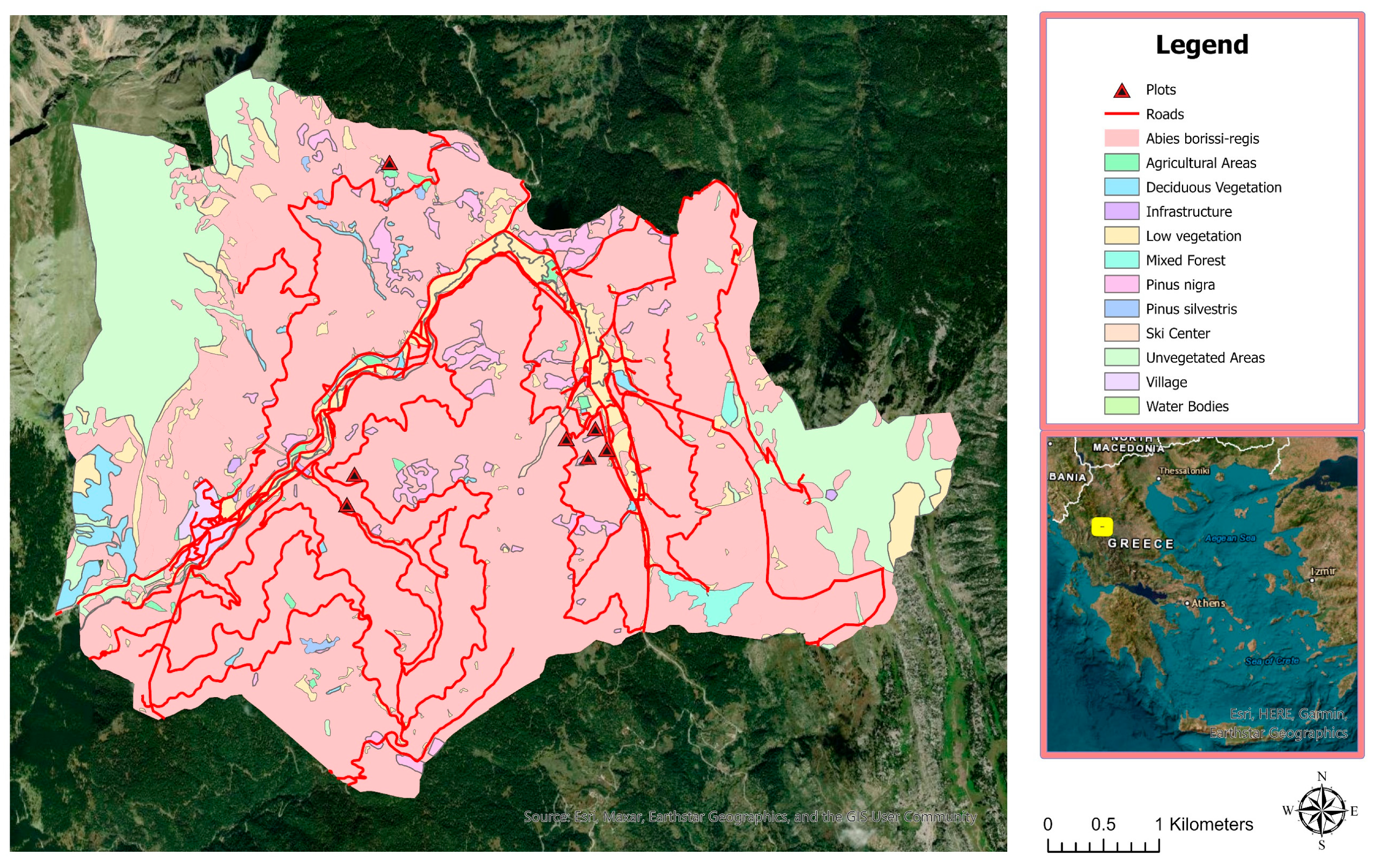
2.1. Study Area

Located on the southeast side of Mount Pindos in Thessaly, Greece, the Pertouli University Forest has been managed by the Aristotle University of Thessaloniki for research and educational purposes since 1934 (Figure 1). Its elevation varies from 1100 to 2050 m above sea level, with steep terrain and an average slope of 28.1 degrees.The climate is characterized as a transitional Mediterranean mid-European climate, featuring warm, dry summers and cold, rainy winters. An uneven distribution of the annual precipitation is observed, with high variability among the seasons. As for the geological substratum, flysch and limestone are the main layers, which along with the mountainous terrain, are vulnerable to weathering and erosion.

Abies borisii-regis, which is a natural hybrid between Abies alba and Abies Cephalonica, is the dominant species in the forested area [70]. The natural stands of this specific species are composed of all-aged stands, including natural regeneration and young trees in the understory, and mature trees in the overstory. Furthermore, it was observed that trees of the same age can exhibit different heights and DBH, which is attributed to the species’ ability to survive under low-light conditions in forest understories for an extended period before being released from overstory light suppression [71]. The remaining forest area is covered by Scots and Black Pines plantations (Pinus silvestris and Pinus nigra) and individual trees of beech, oaks, willows, maple, laburnum and linden.

2.2. Dataset Description

2.2.1. ALS Data

In October 2018, airborne multispectral LiDAR data were acquired over the Pertouli University Forest using a RIEGL VQ-1560i-DW laser scanner sensor mounted on a single-engine airplane. This LiDAR sensor provides a high laser pulse repetition rate that can reach up to 1 MHz per spectral channel and on-the-fly multiple-time-around processing. The data were obtained at an average flight altitude of 2243 m above ground level, with a maximum scan angle of 32°. During the flight, two spectral channels were simultaneously recorded, namely, the green and near-infrared (NIR) (532 nm and 1064 nm, respectively). Before the data delivery, the provider preprocessed the LiDAR data, transforming the full-waveform dataset into discrete returns. The delivered data consisted of a georeferenced point cloud with almost identical point cloud densities for both channels (i.e., 44.65 points/m² for the near-infrared and 44.85 points/m² for the green). Additionally, the simultaneous acquisition of aerial photographs with the LiDAR data provided high-resolution images of the entire forest.

2.2.2. Field Survey

Field measurements were performed in July 2022, including destructive and non-destructive sampling (Figure 2). Destructive sampling was carried out in a specific compartment of a forest, where 13 trees of different characteristics were sampled. Although the field measurements took place 4 years after the LiDAR flight, the differences in tree height, DBH and crown structure were considered to be rather small [72]. Moreover, considering that the Forest Management Plan indicates an annual volume increase of 5.82 m³ ha⁻¹ in three separate growing seasons, the difference in biomass was insignificant.

The selection of the specific sample trees was based on the Forest Management Plan and involved identifying trees with different crown structures, heights and social status, where we aimed to collect representative samples from all forest conditions. A set of tree variables, namely, DBH, tree position, tree height (H), canopy base height and crown radii, were recorded after the felling of each tree. DBH was recorded on the standing trees using a Haglof Mantax Blue caliper (Haglof, Torsång, Sweden), and their locations were determined using a Garmin eTrex 30x touch (Garmin, Lenexa, KS, USA). H, canopy base height and crown radii were measured using a laser distance meter (Leica Disto D2, Leica Camera AG, Wetzlar, Germany). In particular, the length of the above-ground portion of the tree, including the distance between the tree top, the first living branch and the bottom of the trunk, was measured using a laser distance meter. Crown radii were recorded by measuring the distance between the tree stem and the crown edge. The branches (including the needles) were then separated from the tree trunk and divided into 3 sections (dead branches, living branches and tree top). The total fresh weight of each section was weighed on the field using a handheld scale. A sample from each section was collected and transferred to the laboratory for further analysis. For smaller trees with a DBH smaller than 15 cm, the whole crown was taken to the laboratory for needles–branch separation and dry weighting [73]. Needles and branches of the samples were separated to determine the needles/branch ratio and placed in separate bags for drying. All the samples were dried at 85 °C for 72 h and weighed. The ratio of the measured dry weight to fresh weight of the crown components was applied to estimate the total crown biomass (

Table 1. Crown biomass metrics at the single-tree level based on destructive sampling.

Biomass (n = 13)	Mean (kg)	Minimum (kg)	Maximum (kg)
Dead branches	10.62	0.20	32.11
Branches	85.55	1.37	274.75
Needles	49.10	0.72	134.85
Total crown biomass	145.28	3.10	424.10

).

Additionally, non-destructive samples were collected from a set of 200 trees located in representative areas of the forest. This approach was preferred to minimize the disturbance to the forest, due to the invasive nature of destructive sampling. In each sampling region, only trees that were detectable using the LiDAR sensor were measured. The DBH, H, canopy base height, crown radii and position of each tree were recorded. More specifically, the DBH was measured using a Haglof Mantax Blue caliper, H and canopy base height were measured using a Haglof EC II-D electronic clinometer, and the crown radii were measured using a laser distance meter (Leica Disto D2). Tree locations were determined using a Garmin eTrex 30x touch with an average horizontal position accuracy of 6 m. However, only 156 of these trees were correctly identified in the LiDAR point cloud.

3. Methods

The methodology for the LiDAR-based DB, NB and BB estimation, which is described in detail in the following sections (Section 3.1, Section 3.2 and Section 3.3), is illustrated in Figure 3.

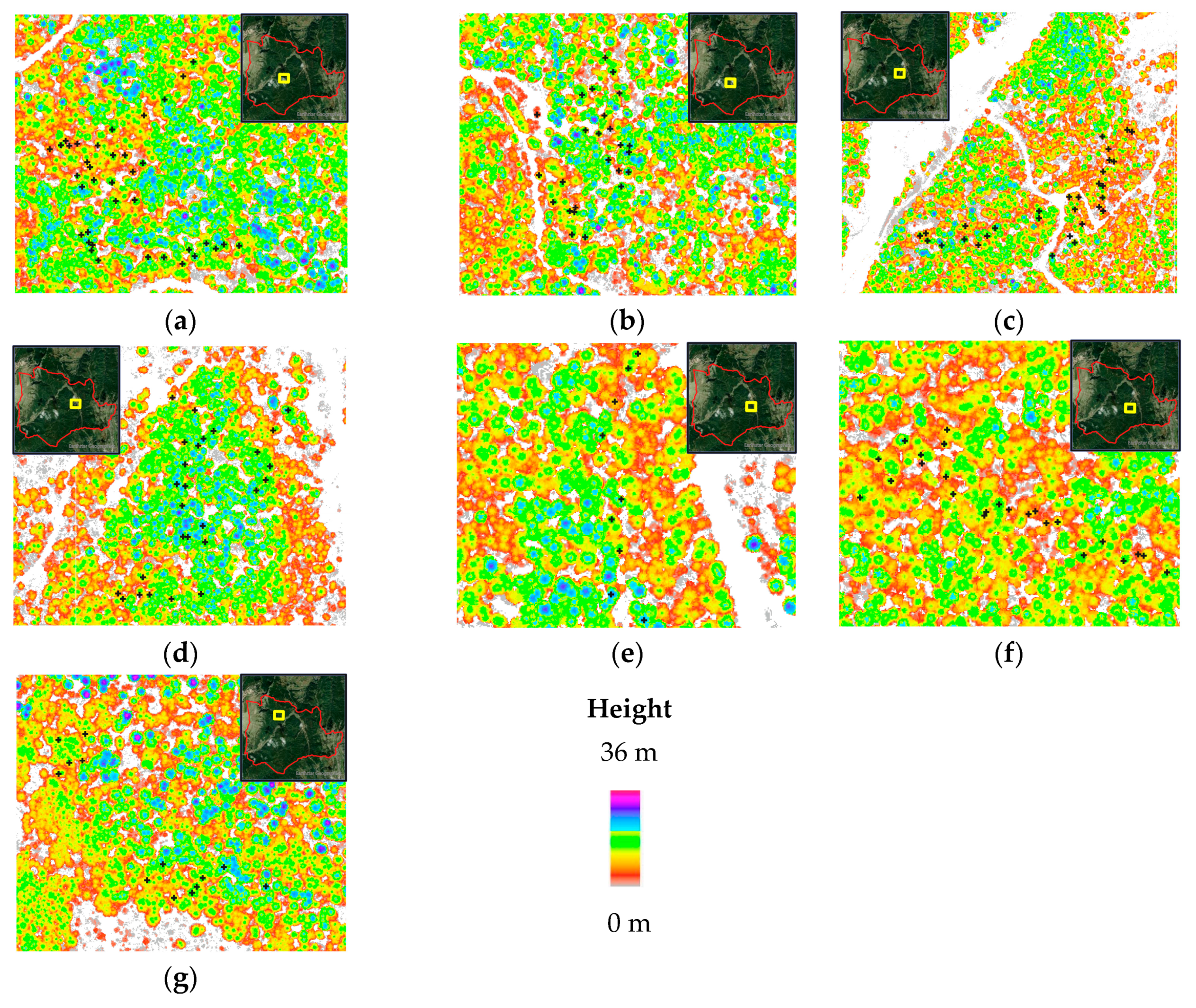
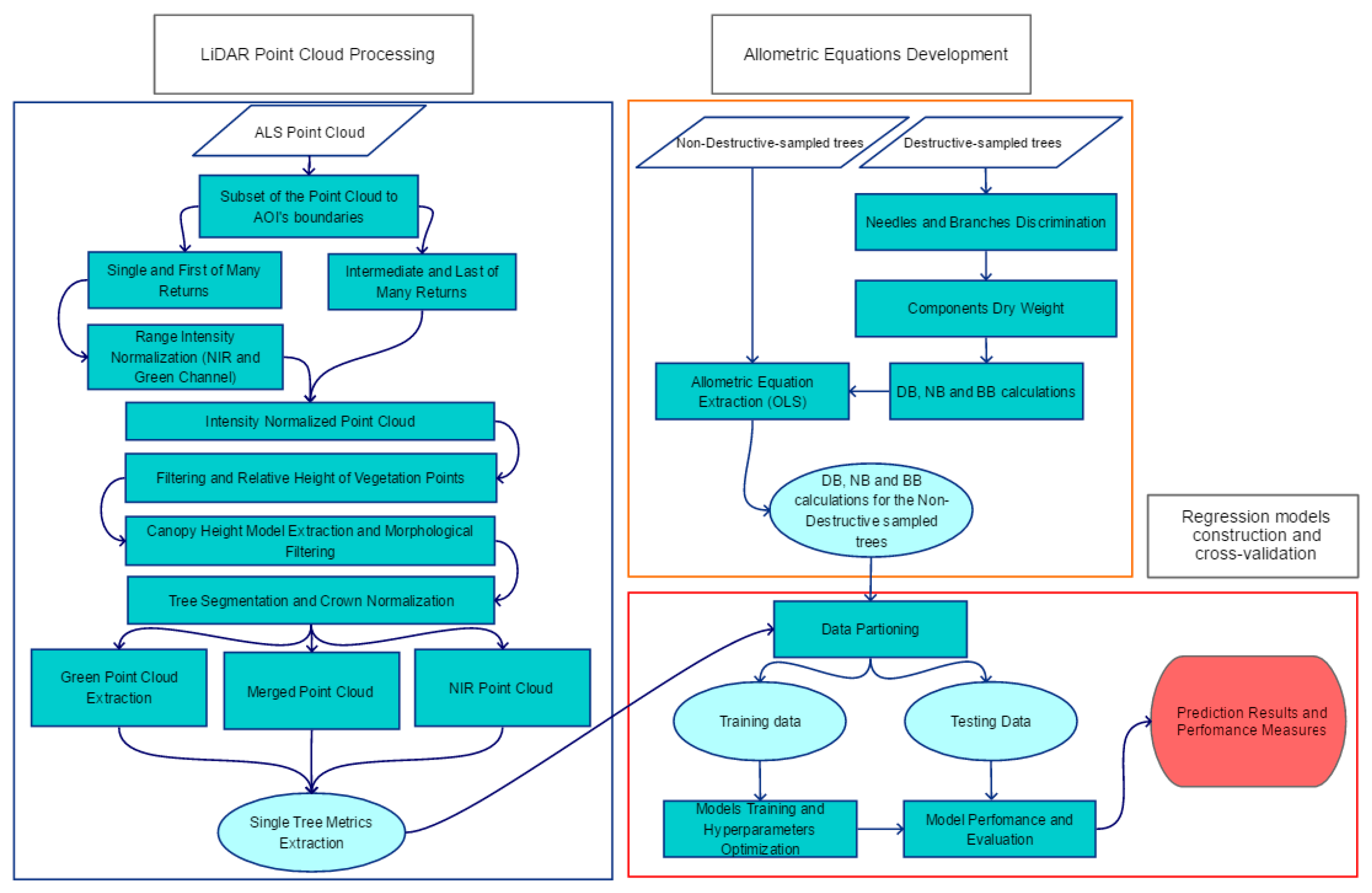
3.1. LiDAR Processing

In order to identify each tree in the LiDAR point cloud and calculate its associate metrics, different processing steps took place using primarily R software, more specifically, the lidR package [74,75].

First, the recorded GPS points from the tree positions were buffered to a 6 m radius, representing the GPS error, and then used to identify the exact field-measured trees in the LiDAR point cloud. The point cloud, divided into green and NIR channels, was clipped to the buffered areas and employed for further processing. Since the study area was characterized by mountainous terrain and irregular forest canopy, a large intensity variability was expected. The single and first-of-many returns were significantly stronger than the intermediate returns and, in most cases, located higher in the canopy. Consequently, the disparity in their intensity values was influenced by the different vegetation materials (i.e., foliage and wood) that obstructed the pulse [76]. Hence, the single and first-of-many returns of both green and NIR channels were solely used for the range intensity normalization procedure.

Regarding the calibration parameter f in the range normalization procedure, values between 2 and 2.5 are considered more suitable for forested areas [77]. In this study, the reference range parameter was set to the average flight altitude and f as 2.0, according to the radar theory [78]. After the intensity normalization, the normalized point clouds were joined with the intermediate and last returns of each channel. The combination of both the intensity-normalized and not normalized echoes (i.e., the intermediate and last returns) was used to reconstruct the initial point cloud and extract height- and intensity-related metrics for the crown components estimation.

The normalized point cloud was filtered for noise removal, using the Statistical Outliers removal algorithm [79], and classified into ground and non-ground points using the Cloth Simulation Algorithm [80]. The ground-classified points were interpolated to construct the digital terrain model (DTM), using the triangulated irregular network (TIN) algorithm, which was employed for the point cloud normalization. The canopy height model (CHM) was subsequently produced, employing the Pit-free algorithm [81]. The Pit-free algorithm was selected due to its ability to provide accurate tree delineations, especially in high-density LiDAR data. Both rasters (i.e., DTM and CHM) had the same resolution of 0.42 m, which was defined based on the nominal pulse spacing [82]. Subsequently, to reduce the over-segmentation phenomenon due to the complex forest canopy, a morphological erosion with a cross-shaped structuring element was applied to the CHM.

Several methods have been proposed for automatic crown delineation [47,69,83], however, large omission and commission errors are often observed [61]. In this study, watershed segmentation was employed for the crown delineation procedure, without providing treetops or any kind of local maxima feature. Although the watershed algorithm outperformed the other tested algorithms [47,83], providing accurate segmentation results, manual corrections were applied where necessary.

According to [84], slopes can significantly impact the normalized canopy height of individual trees, affecting the crown of each tree. Therefore, considering the mountainous terrain of the study area, the elimination of the terrain effects for each tree was essential for accurate crown biomass estimation. Consequently, a crown normalization process inspired by the P-trees algorithm [45] was employed.

Taking into account the positional error of the GPS position for determining each tree’s position and the horizontal accuracy of the point cloud, the errors were expected to be 6 m and 0.30 m respectively [51]. To match the field-measured trees with the segmented trees in the point cloud, a candidate-searching approach was employed, similar to the one of [85]. Within each buffer zone, the highest point in each segmented tree was assigned as the tree top. Segmented trees with a height difference greater than 1 meter from the field-measured height were directly eliminated and the remaining trees were used as candidate trees. Additionally, field observations and very-high-resolution aerial photographs were used to identify the actual tree measured on the field among the candidate trees according to the method described in [86]. As a result, 156 out of 200 non-destructively sampled trees were successfully identified in the LiDAR point cloud. Finally, the point cloud for each channel (i.e., green, NIR and merged) was extracted in order to calculate the LiDAR-derived height and intensity metrics separately (

Table 2. Summary of the LiDAR-derived metrics calculated for the crown biomass estimation. All described metrics (height- and intensity-related) were extracted for each point cloud separately (merged, NIR and green). Height bincentiles refer to the cumulative percentage of points in a percentage of the total height, while percentiles represent the distribution of the vertical structure between the highest and lowest height. The intensity-related metrics were obtained using only the first-of-many and single returns.

LiDAR Metrics	Description
p10, p20, …, p95, p99	Height percentiles
b10, b20, …, b95, b99	Height bincentiles
max	Max height
avg	Average height
std	Height standard deviation
int_p10, int_p20, …, int_p99	Intensity percentiles
int_std	Intensity standard seviation
int_avg	Average intensity
int_skew	Intensity skewness

).

3.2. Allometric Equations

Several allometric models have been developed over recent decades for the estimation of the biomass of different tree components [73]. Crown biomass is usually calculated using the DBH and H as inputs in empirical allometric equations, providing predictions for validating biomass estimates from remote sensing models [87]. However, no allometric equations are available for crown or crown components biomass in Abies borissi-regis. In this study, new “intrinsically linear” allometric equations were created, using 13 destructively sampled trees, for dead branches, needles and branches biomass (Equation (1)):

$$\ln \left({\mathrm{B}}_i\right)=a_i+b_{i1}\times \ln \left(DBH\right)+b_{i2}\times \ln \left(H\right)+{\epsilon }_i$$

(1)

where B is the biomass of each component; a and b are the intercept and scaling coefficient, respectively; and ε is the residual error. The constructed equations were based on DBH and H, as the other field measurements were found to be insignificant (i.e., crown base height, and crown radii). The originally selected sample size was decreased from 25 to 13 according to the guidelines of the local forest service, due to the potential damage from the fallen trees and the sampling procedures to the understory. In fact, previous studies that focussed on allometric equations for biomass components estimation reported similar sample sizes to ours [10,73,88,89,90]. Subsequently, a sample size of 13 was considered suitable for our study as well.

As a result, the measured DBH and H of the non-destructively sampled trees were employed in the allometric equations to calculate the DB, NB and BB for each tree. The results were used as reference biomasses for each crown component. For these equations, no conversion factor was required, as they were used to directly estimate the biomass in kg/tree. The performance of the allometric equations was evaluated based on the relative square error (RSE), R² and adjusted R² (adjR²).

3.3. Crown Biomass Estimation Using Regression Algorithms

To assess the predictive potential of the LiDAR-derived metrics for accurate DB, NB and BB estimation, three different regression algorithms were tested, namely, random forest (RF), support vector regression (SVR) and Gaussian process (GP). Prior to the analysis, the predictors were “center” scaled and divided into training (75%) and testing (25%) sets. In addition, a nested ten-fold cross-validation with grid search was applied in each training set to obtain the training accuracy and the optimal hyperparameter values for each model. This cross-validation method eliminates the bias that may be introduced by the simple cross-validation approach, providing a more reliable criterion for choosing the best model [91]. The regression models were validated to an independent testing set (i.e., 25% of the total number of samples), which was randomly split from the training data to obtain the predictive performance of each algorithm. Assessment of all models’ performance for each crown biomass component estimation was carried out based on the mean absolute error (MAE), mean square error (MSE), bias, relative mean square error (RMSE) and R². In addition, the relative importance of individual predictors in each model was calculated using a model-agnostic procedure, providing a list of the ten most important variables for each model [92].

3.3.1. Random Forest

The random forest algorithm is a flexible machine learning technique that utilizes multiple randomized decision trees to carry out tasks such as classification and regression [93]. According to this approach, each decision tree is trained on a different bootstrap sample of the data, and the predictor variables at each node are randomly selected [94]. Concerning the model’s tuning, two hyperparameters were tuned, namely, the number of trees to grow and the number of predictors for each tree. A variable number of trees to be grown was tested, ranging from 50 to 500 with a step size of 50, and variable numbers of predictors for each tree were defined as the number of predictors divided by three [95].

3.3.2. Support Vector Regression

This method, traditionally known as support vector regression (SVR), was initially developed by Vapnik [96] as an extension to the traditional SVM algorithm [97]. The goal of this method is to find a function f(x) among the pairs of the training data without considering the pairs that have a larger deviation from the support vector than an ε deviation [98]. The ε-SVR algorithm was applied in our study, where the input data were transformed into a high-dimensional feature space using a nonlinear function, solve the final model by minimizing the training error and the complexity of the model [99]. In our work, the rbf kernel was employed and two hyperparameters were optimized, namely, the cost of violation of restrictions and sigma parameter.

3.3.3. Gaussian Process

The Gaussian process is a probabilistic machine learning framework that is widely used for regression and classification tasks [100]. In regression problems, a Gaussian process regression model can make predictions by incorporating prior knowledge (kernels) [101] find the probability distribution that best describes the data [102]. According to this method, it is assumed that the input data follow a multivariate Gaussian distribution, while the noise is considered independent of the data [103]. In this study, the radial basis function (rbf) kernel was employed, and the sigma inverse width parameter was optimized using a grid search.

4. Results

In this study, DB, NB and BB were estimated using three different algorithms. In particular, new allometric equations were developed and evaluated for their accuracy to enrich the reference dataset with non-destructive samples (Section 4.1). Subsequently, three regression algorithms (i.e., RF, SVR and GP) were evaluated for their potential to reliably estimate DB, NB and BB. The results are presented in detail in the following sections (Section 4.2, Section 4.3 and Section 4.4).

4.1. Allometric Equations

Regarding the allometric equations, 13 trees were destructively sampled in the field to develop a different equation for each DB, NB and BB estimation. All the developed models were based on the use of DBH and H measurements.

Table 3. Parameter, residual standard error (RSE), R² and adjusted R² values for the single-tree dead branch, needle and branch biomass (DB, NB and BB, respectively) estimations based on DBH and H. Parameter a is the intercept, while parameters b and c are the coefficients of H and DBH, respectively.

Equation	Parameter	RSE	R2	adjR2
Dead branches biomass	a = −0.5300 b = 1.3173 c = 0.8949	0.8526	0.7209	0.6651
Needles biomass	a = −1.9486 b = 2.2666 c = 0.6815	0.4811	0.9311	0.9173
Branches biomass	a = 1.1006 b = 1.5938 c = 1.2820	0.5137	0.9244	0.9093

presents the results of the allometric DB, NB and BB estimation models. Among the three models, the NB model showed the greatest accuracy, with R² and adjR² being 0.93 and 0.91, respectively. The DB model resulted in lower R² and adjR² values and the largest RSE. The lower accuracy of the DB allometric equation compared with the others can be attributed to the natural pruning of the fir, which is inconsistent and significantly varies between trees of different ages, social statuses, competitions and lighting conditions.

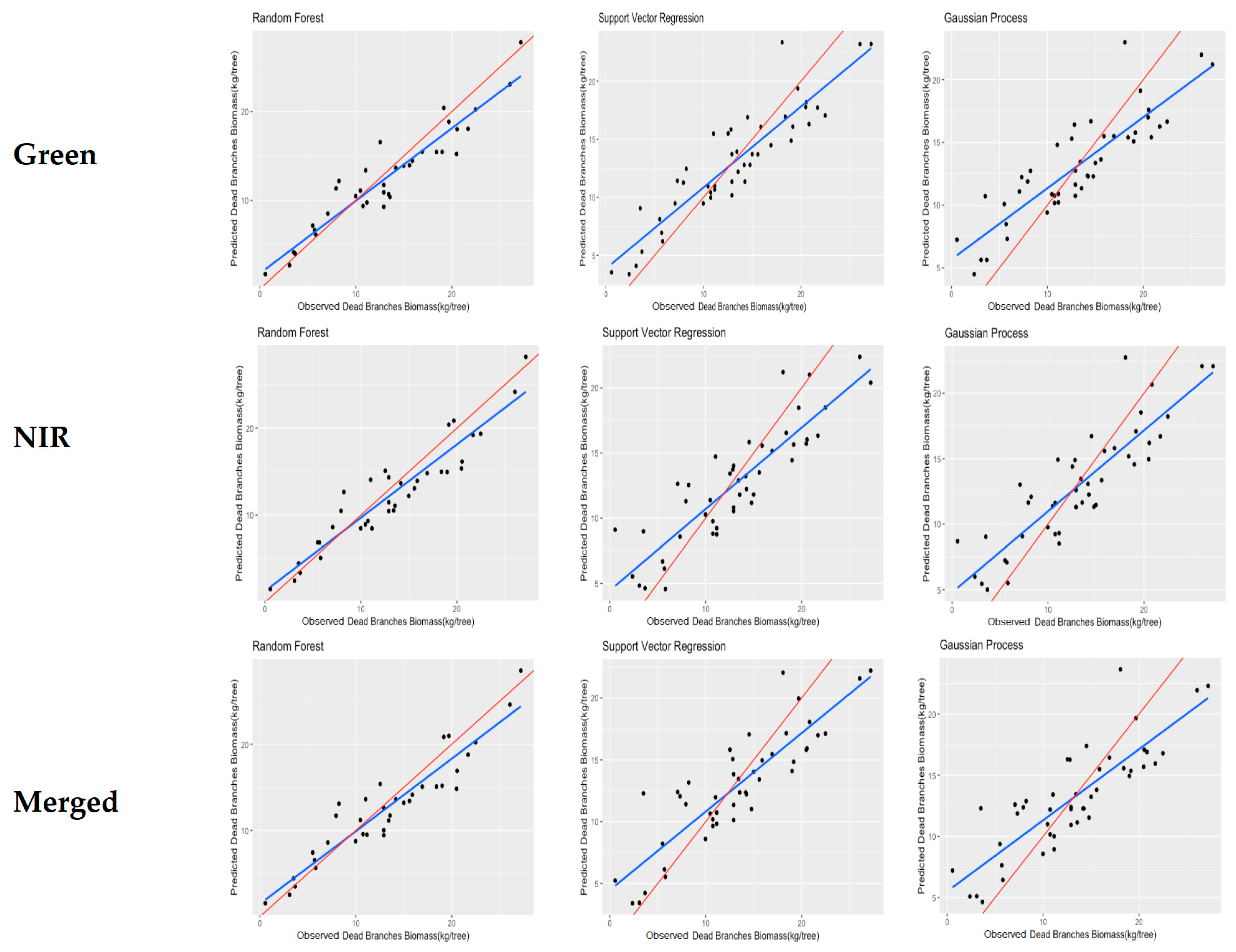
4.2. Dead Braches Biomass

The performance of the models for DB estimation using the multispectral LiDAR data (i.e., green, NIR, and merged) is presented in

Table 4. Testing the performance results of the utilized algorithms for the dead branches biomass (DB) estimation using multispectral LiDAR data based on 46 testing samples.

Point Cloud	Model	MAE	MSE	rbias	RMSE	RMSE%	R2
Green	RF	1.92	5.30	−0.04	2.30	17.45	0.89
	SVR	2.28	7.53	−0.19	2.74	20.98	0.82
	GP	2.78	11.28	−0.38	3.35	25.67	0.75
NIR	RF	2.10	5.77	−0.01	2.40	18.20	0.88
	SVR	2.56	10.00	−0.38	3.16	24.18	0.77
	GP	2.62	10.17	−0.40	3.18	24.37	0.76
Merged	RF	2.00	5.67	−0.03	2.38	18.05	0.87
	SVR	2.54	10.28	−0.25	3.20	24.51	0.75
	GP	2.88	12.13	−0.38	3.48	26.62	0.71

. Figure 4 depicts the model’s fit, showing the difference between the regression and the hypothetical 1:1 lines. Overall, the models demonstrated satisfactory predictive performance, with R² values greater than 0.7 and RMSE% values lower than 26%.

More specifically, the RF algorithm provided the best results compared with all of the other algorithms in all three different point clouds (i.e., green, NIR and merged), with the green achieving an R² of 0.89, MAE of 1.92 kg, rbias of −0.04 and RMSE% of 17.45. The RF algorithm produced a similar estimation performance in the other two point clouds (i.e., NIR and merged) in terms of R², MAE, MSE and RMSE; however, the NIR produced the lowest rbias. The application of the SVR algorithm achieved the second-best performance among all of the point clouds, with the green providing the best predictions in terms of R² (0.82), RMSE% (20.98), rbias (−0.19) and MSE (7.53 kg). The SVR in the NIR and merged point clouds resulted in similar predictive performance, as evidenced by the R² (0.77 and 0.75, respectively) and RMSE% (24.18 and 24.51, respectively); however, the merged achieved a lower rbias compared with the NIR (−0.25% and 0.38%, respectively). The GP model provided the lowest performance, with an R² of 0.71 and RMSE% of 26.62 in the merged point cloud. A slight improvement in terms of R², RMSE and MSE is observed in the NIR and green, although the MAE and rbias were almost identical in all cases.

Regarding the relative predictors’ importance for the DB estimation (Figure 5), the best-performing algorithm indicated the max as the most important variable, followed by the p99, p95, p90 and p80. The same five height percentiles were selected as the most important variables by the RF algorithm in all of the point clouds. The b80, b70 and avg were also identified among the ten most important variables. It can be observed that the height metrics related to the upper sections of the crown (e.g., max, p99 and p95) were considered more important compared with those from the lower canopy. However, two metrics that corresponded to the lower parts of the crown, namely, p10 and p20, were also selected among the most important variables in all of the point clouds.

Overall, it is evident that all three point clouds resulted in similar DB estimation accuracies using the RF algorithm, which was identified as the most reliable in terms of R² and RMSE. In addition, the significance of the height-derived LiDAR metrics was considered higher compared with those of the intensity metrics, as no intensity metrics were identified among the most valuable for the DB estimation.

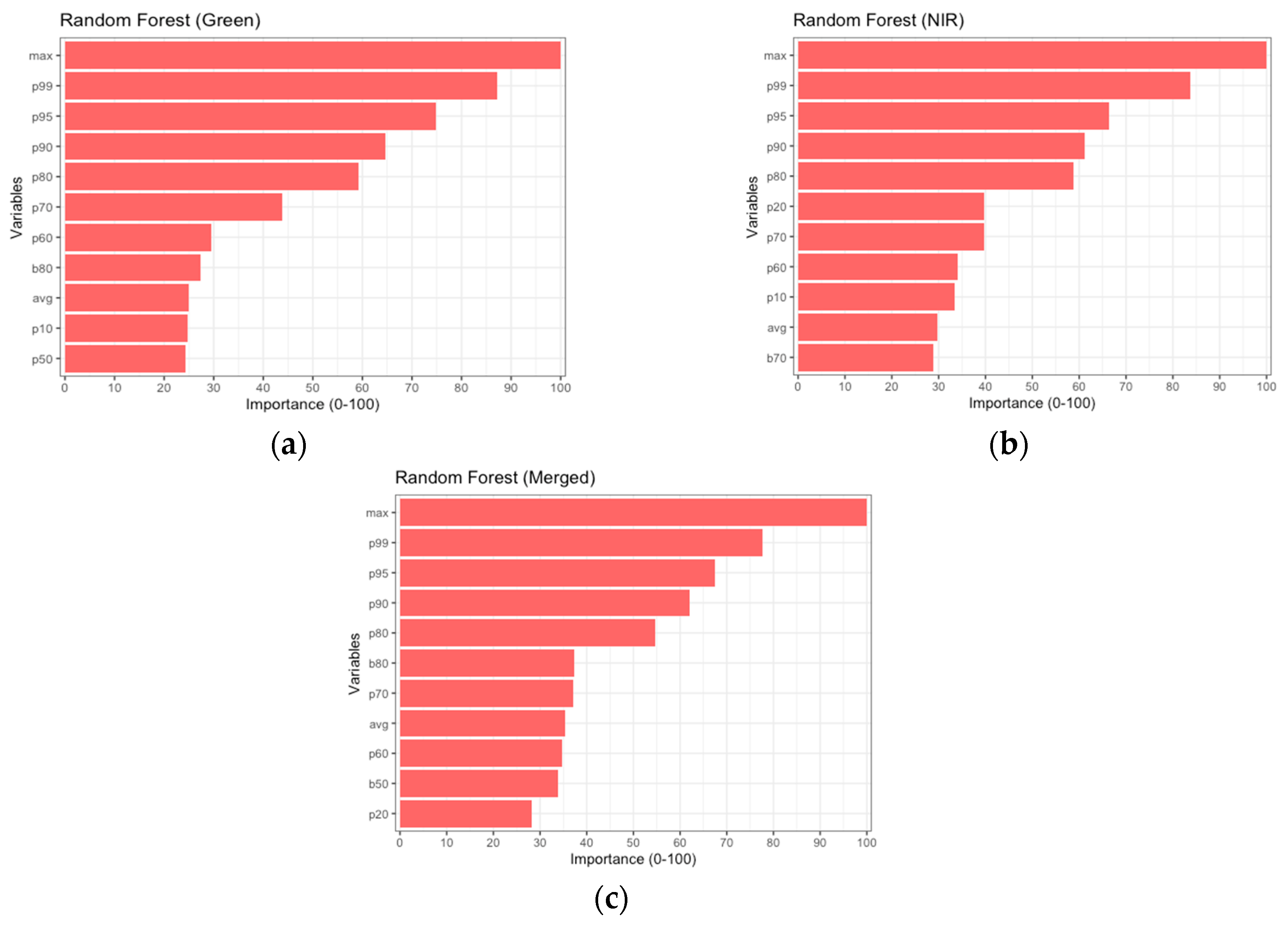
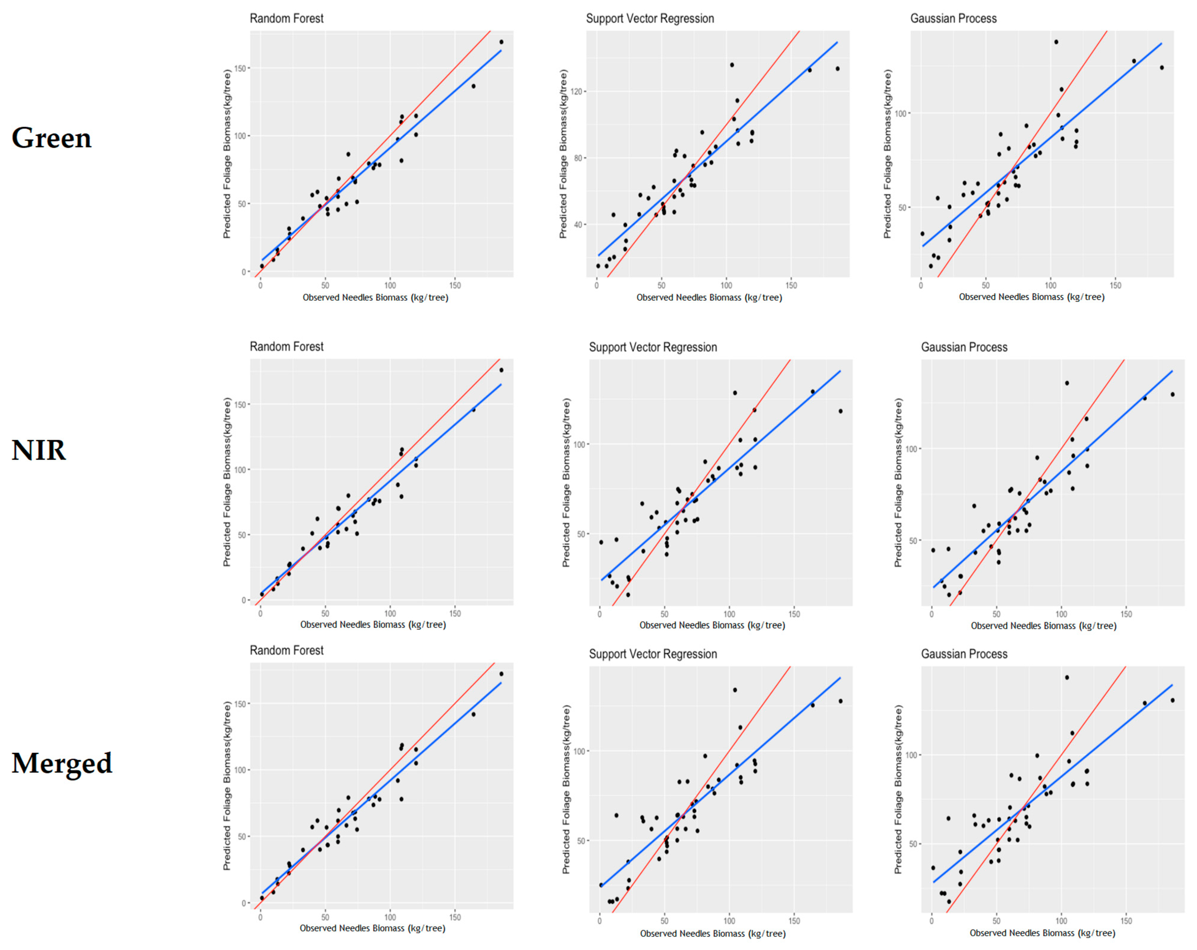
4.3. Needles Biomass

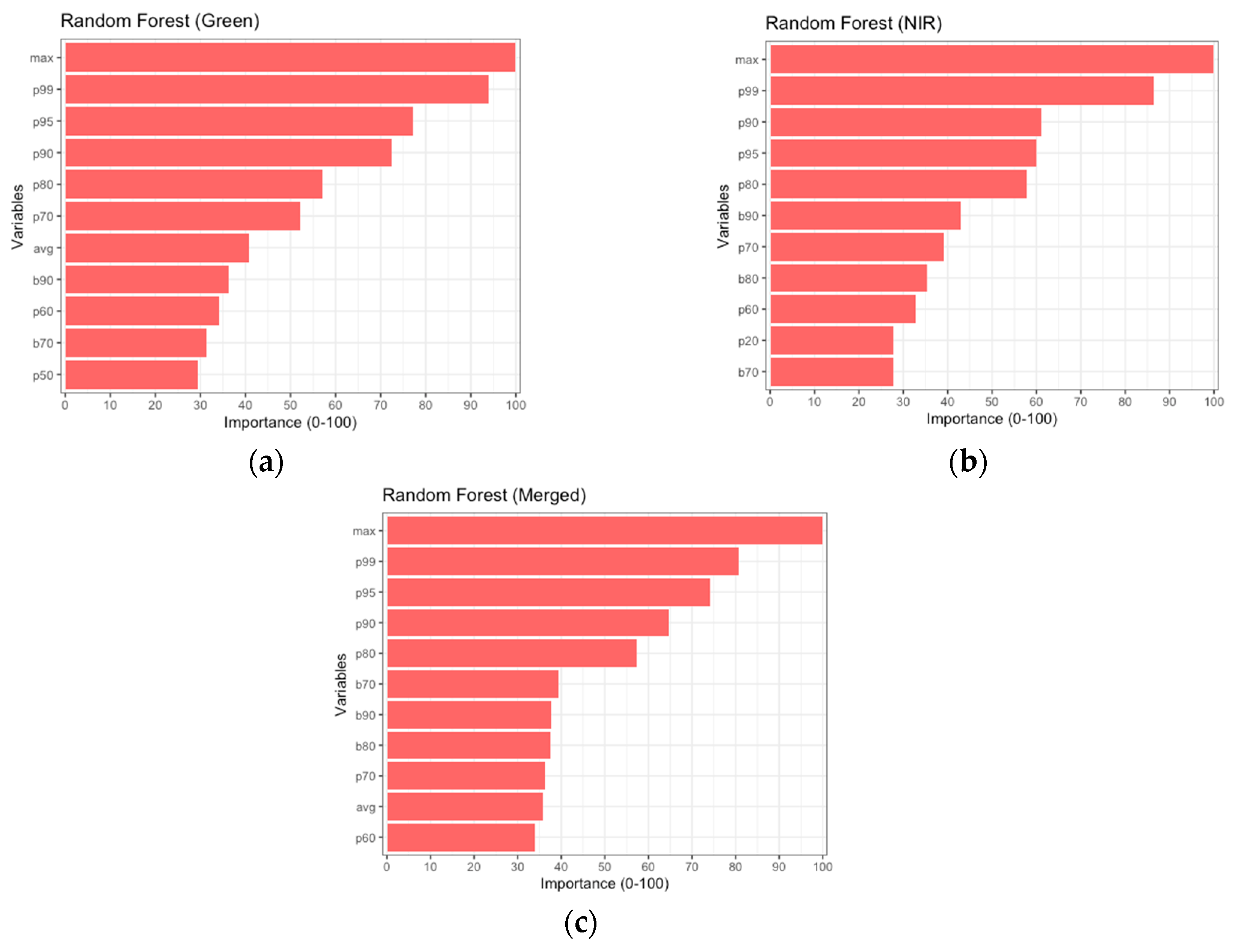
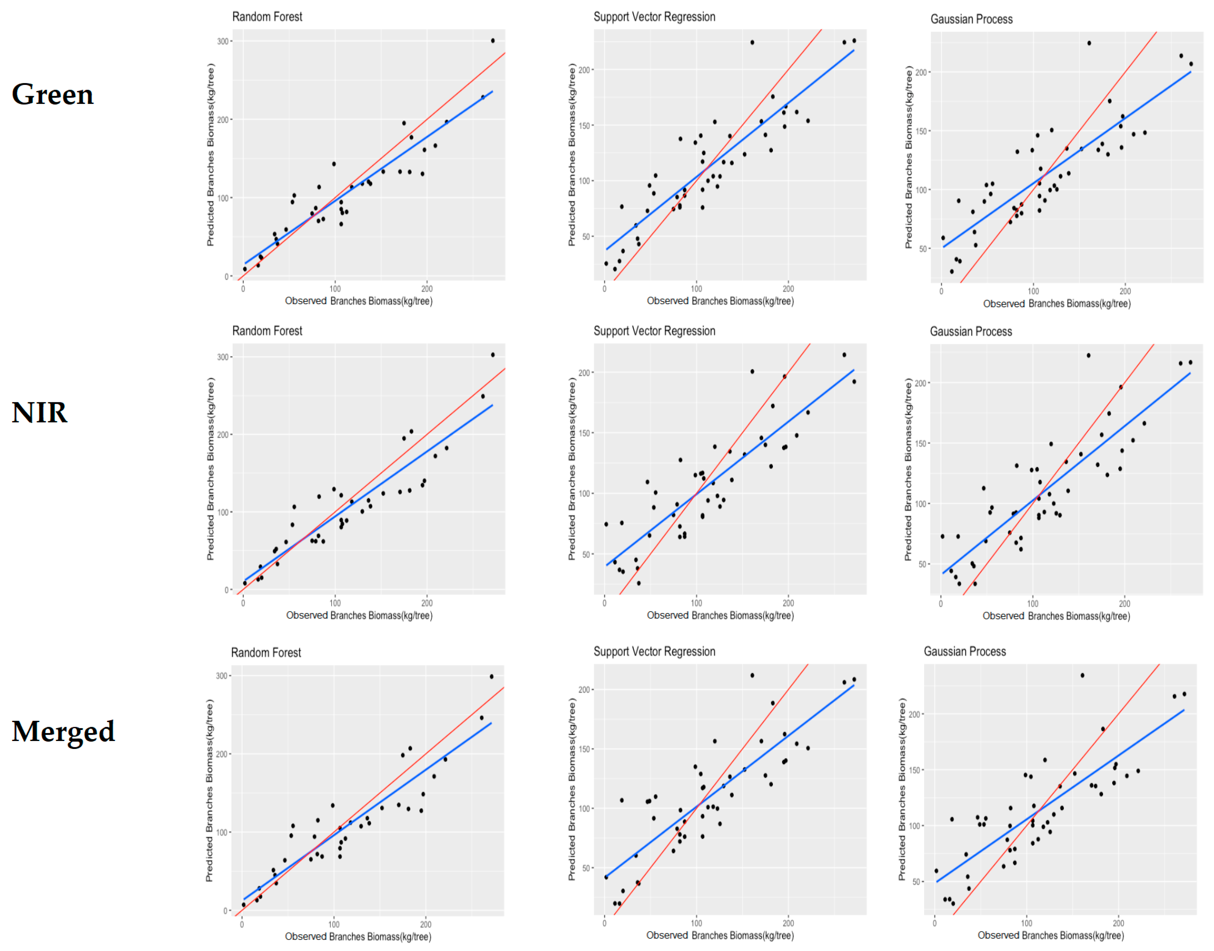
The performance of the three different regression algorithms for NB estimation using the multispectral LiDAR data (i.e., green, NIR, and merged) is presented in this section (

Table 5. Testing performance results of the utilized algorithms for the needles biomass (NB) estimation using multispectral LiDAR data based on 46 testing samples.

Point Cloud	Model	MAE	MSE	rbias	RMSE	RMSE%	R2
Green	RF	9.24	139.73	−0.06	11.82	17.31	0.93
	SVR	12.70	278.38	−0.43	16.68	24.69	0.84
	GP	15.59	428.24	−0.93	20.69	30.62	0.76
NIR	RF	9.71	135.98	−0.06	11.66	17.08	0.93
	SVR	13.82	363.06	−1.05	19.05	28.19	0.8
	GP	14.26	354.35	−1.06	18.82	27.85	0.8
Merged	RF	9.48	131.69	−0.05	11.47	16.80	0.93
	SVR	14.48	382.71	−0.65	19.56	28.95	0.78
	GP	16.54	451.00	−0.95	21.23	31.42	0.73

). Additionally, the models’ fit for each channel is illustrated in Figure 6, showing a comparison between the regression and the hypothetical 1:1 line.

The NB models displayed an increase in R² and significantly higher RMSE% and MSE metrics in comparison with the DB models. More specifically, using RF on the merged point cloud resulted in the highest R² (0.93) among all the algorithms, with a low MSE (131.69 kg), rbias (−0.05%) and RMSE% (16.80%). Although the R² values of the RFs using the three point clouds were identical, the lowest MAE (9.24 kg) was observed in the green. Contrary to the RF algorithm, the SVR provided better NB predictions in the green, with an R² of 0.84, MAE of 12.70 kg, MSE of 278.37 and RMSE% of 24.69%. The same algorithm resulted in significantly worse predictions in the NIR and merged, with R² values of 0.8 and 0.78, MSE values of 363.06 kg and 382.06 kg, and RMSE% values of 27.85% and 28.95%, respectively. The GP model provided the lowest performance, with an R² of 0.73 and the highest RMSE% of 31.42% in the merged point cloud. This algorithm provided slightly improved results in the green and NIR, with the NIR achieving the highest R² (0.8), an RMSE% of 27.85% and an MAE of 14.26 kg.

The relative predictor importance of the best-performing model for NB is presented in Figure 7. Similar to the RF model for DB estimation, the max was indicated as the most important variable, followed by the p99, p95, p90 and p80. More specifically, in the green, the RF model identified the aforementioned variables, along with p70, b70, avg and b90. These variables were considered significant in all of the models; however, their importance values were significantly lower than the first five (i.e., max, p99, p95, p90 and p80). Overall, it can be observed that the merged point cloud could provide reliable NB estimates using primarily height-derived LiDAR metrics, resulting in significantly lower MSE and RMSE values.

4.4. Branch Biomass

The performance of the developed models for BB estimation using the multispectral LiDAR data (i.e., green, NIR and merged) is presented in

Table 6. Testing performance results of the utilized algorithms for the branches biomass (BB) estimation using multispectral LiDAR data based on 46 testing samples.

Point Cloud	Model	MAE	MSE	rbias	RMSE	RMSE%	R2
Green	RF	22.57	754.17	−0.13	27.46	24.09	0.85
	SVR	26.11	1002.14	−0.47	31.65	28.21	0.79
	GP	30.91	1390.12	−0.96	37.28	33.23	0.72
NIR	RF	24.61	831.86	−0.09	28.84	25.30	0.84
	SVR	28.88	1245.91	−1.05	35.29	31.46	0.75
	GP	28.95	1237.37	−1.07	35.17	31.35	0.74
Merged	RF	23.46	812.13	−0.11	28.49	25.00	0.84
	SVR	28.95	1338.87	−0.67	36.59	32.61	0.71
	GP	31.89	1491.21	−0.97	38.61	34.42	0.67

. Additionally, the models’ fits are illustrated in Figure 8.

In particular, among the different algorithms and channels, the RF model using the green provided better performance for BB estimation (i.e., R² = 0.85, RMSE% = 24.09% and MAE = 22.57 kg). The RF models using the other two point clouds (i.e., NIR and merged) marginally outperformed the green one, with an almost identical R² of 0.84, MSE of 831.86 kg and 812.13 kg, and RMSE% values of 25.30% and 25.00% for the NIR and merged, respectively. Excluding the RF models, the SVR using the green was the second-best-performing model, with an R² of 0.79 and RMSE% of 28.21% compared with the other channels, with R² values of 0.75 and 0.71 and RMSE% values of 31.46% and 32.61% for the NIR and merged, respectively. Contrary to the aforementioned models, the GP model provided better estimations using the NIR channel in terms of R² (0.75), RMSE% (31.35%) and MAE (28.95 kg), resulting in marginally lower results compared with the SVR model using NIR. Finally, the GP model using the merged achieved the lowest R² (0.67) and the highest RMSE% (34.42%) compared with the rest of the employed algorithms.

The relative predictor importance of the best-performing algorithms for BB estimation in each channel is illustrated in Figure 9. Similar to the DB and NB, the RF model indicated primarily height-derived LiDAR metrics as the most important variables for reliable biomass estimation. More specifically, the max, followed by the p99, p95, p90 and p80, were identified among the most important variables. More specifically, the RF model using the green identified the aforementioned variables, along with p70, avg, b80, p60, p10 and p30. Using the NIR, the RF identified p10 as the fifth most significant variable, which corresponded to the lower parts of the crown. Regarding the merged, the selected variables were almost identical to the green; however, the max presented a significantly higher importance value compared with the other variables.

Overall, it is evident that the RF could provide accurate BB estimates using any of the three channels, resulting in remarkably higher R² and lower RMSE values compared with the SVR and GP models.

5. Discussion

In the present study, we examined the performance of three machine learning approaches using multispectral LiDAR data for single-tree crown components biomass estimation in a multilayered fir forest. More specifically, new allometric equations were constructed based on destructive sampling for DB, NB and BB estimation, as no equations were available for the specific species. Thus, the DBH and H were measured in the field and used as input data in the developed allometric equations to generate reference DB, NB and BB estimates. These reference data were subsequently employed for the tree level DB, NB and BB estimation using three different regression algorithms (i.e., RF, SVR and GP). LiDAR-derived height and intensity distribution metrics at the tree-level from both spectral channels (i.e., green and NIR) were employed as potential independent variables in the predictive models. Overall, the results indicate that the biomass of all crown components could be reliably estimated using either of the three regression algorithms, however, the RF models provided the best predictions in all cases.

In the case of the DB estimation, the RF model using the green point cloud resulted in the best estimation performance in terms of R², MAE, MSE and RMSE (i.e., R² = 0.89, MAE = 1.92 kg, MSE = 5.30 kg and RMSE = 2.30 kg) (Table 4). It is noteworthy that only height-derived metrics were selected as the most important variables for DB estimation, which indicates the significance of the height-related metrics for crown biomass estimation. Hence, intensity information, which represents the canopy’s surface reflectivity, is considered uncorrelated with the DB. Taking into consideration the fact that the dead branches in fir species are concentrated in the lower parts of the canopy, height metrics representing the lower crown should be selected among the most variables for DB estimation. However, height metrics related to the upper-crown parts (i.e., max, p99, p95, p80 and p70) were the most important variables in the best-performing models, while the p20 and p10 were considered less important. This can be attributed to the fact that the tree height, which is closely correlated with the maturity of the tree, has a significant impact on DB [104]. A comparison between the different algorithms revealed that the monospectral data derived from the green channel could provide an accurate dead branches biomass estimation, which was credited to the higher sensitivity of this channel in the woody parts of the tree [105]. Although the multispectral LiDAR data are considered valuable for accurate species classification [66], forest biomass [106] and fuels estimation [37], it is evident that the exclusive use of monospectral data can provide reliable DB estimations.

With respect to NB estimation, the RF presented the highest values of the statistical evaluation measures (i.e., MAE, RMSE and R²). As opposed to the DB, the RF produced almost identical estimation performances using the green, NIR and merged point clouds (Table 5). As for the variable importance, the selected variables consisted primarily of height-derived metrics, similar to the DB models (Figure 7). More specifically, max, p99, p95, p80, p70 and avg were selected as the most important variables, showcasing the importance of height-related metrics in reliable NB estimation. This can be considered a rather logical association since the vast majority of living branches are found in the upper canopy.

Regarding the BB estimation, the RF models resulted in similar R², MAE, RMSE and rbias in all of the channels. In particular, the RF in the green channel provided the highest R², with low MAE, MSE and RMSE% values (R² = 0.85, MAE = 22.57 kg, MSE = 754.17 kg and RMSE% = 24.09%) (Table 6). The GP provided the worst R² among all crown components (0.67), with high MAE and RMSE values (MSE = 1491.21 kg, RMSE% = 34.42%). Similarly to the previous crown biomass components, height-derived metrics (i.e., max, p99, p95, p90, p80 and p10) were primarily identified as the most important variables for BB estimation.

All models used in this study demonstrated satisfactory prediction accuracy for DB, NB and BB, with the RF presenting the highest values in terms of R², RMSE and MAE. The RF is a non-parametric regression method that provides robustness and flexibility in modeling individual tree attributes with high accuracy [35]. Moreover, the RF algorithm has a significant advantage over the other machine learning algorithms, as it can effectively handle collinearity and nonlinear regression problems [52]. Overall, the results demonstrate that DB, NB and BB could be reliably estimated in a multilayered forest using the RF algorithm.

Although AGB estimation using LiDAR data is becoming increasingly popular, only a few studies have focused on crown biomass estimation. Furthermore, the majority of the studies focused on plantations and semi-natural forests, which are significantly different from natural forest biomes. However, no studies have yet explored the potential of LiDAR in DB estimation. Consequently, we compared our NB and BB results to similar reports that exploit both single-tree and plot-based approaches, in either forest type. In 2013, [107] employed LiDAR data for biomass components estimation in an evergreen-dominated forest with mountainous terrain in western China. The results showed a lower R² (0.757) in terms of BB compared with ours; however, the RMSE% was significantly lower (12.423%). Regarding the NB, the reported R² (0.36) was significantly low compared with the one reported in this study. Hauglin et al. [6] estimated the single-tree branch biomass of Norway spruce using LiDAR data, incorporating height- and intensity-derived LiDAR metrics. Although the results are marginally inferior compared to ours in terms of R² (0.83), we achieved a significantly lower RMSE% (45%). In addition, [62] used linear models with logarithmic transformations to estimate NB and BB in a coniferous forest, reporting a lower R² and higher RMSE% compared with ours in both cases. The variation in the results can be attributed to the different algorithms and LiDAR sensors used, as well as the significant difference between the species of each study area.

Even though the aforementioned studies employed both intensity- and height-derived LiDAR metrics, none of the above utilized multispectral LiDAR for the crown components biomass predictions. In this study, we evaluated the potential of different LiDAR channels (i.e., green, NIR and merged) to estimate DB, NB and BB. According to our findings, the monospectral data can provide accurate crown components estimations, and in most cases, the predictions were superior compared with the multispectral data. More specifically, the green channel provided the best BB, NB and DB predictions using either of the three regression algorithms. The merged point cloud produced the lowest evaluation measures of all crown components, which can be attributed to the large complexity of the point cloud. Considering that the monospectral point cloud density was already high (~44.65 points/m²) for AGB estimation at the individual tree level, the additional channel could not provide any supplementary information to improve the predictions of crown biomass. Furthermore, the intensity information of both channels was not found to be significant for the estimation of the crown biomass components. However, multispectral LiDAR and intensities can contribute to the classification of different tree species, which is essential for biomass estimation, especially in mixed forests [108].

Although this research reached its objectives, there were some inherent constraints. First of all, the destructive sample used in the study may be deemed insufficient for a forest with such a complex structure, leading to potential uncertainty in the predictions [37]. Nevertheless, the majority of studies employ similar sample sizes for destructive sampling [73], enriching the reference data via allometric equations. Regarding the dead branches, our approach did not take into consideration the lighting conditions or suppression caused by neighbor trees, which constitute major factors for the natural debranching. In addition, the study focused on dominant and co-dominant trees, excluding all the understory trees, which have a significant role in carbon allocation. As a result, the methodology can be transferred in similar biomes for DB, NB and BB, providing estimations only for the dominant and co-dominant trees.

In summary, our research shows that LiDAR data are capable of providing accurate crown components biomass predictions in a multilayered fir forest. This study emphasized the importance of using monospectral LiDAR-derived height metrics for crown biomass estimation, which is crucial for forest inventory management and forest biomass dynamics, as they comprise the majority of the logging residues. It should be noted that this research was the first contribution for dead branches biomass estimation using primarily airborne LiDAR data at the single-tree level, and one of the few studies employing LiDAR data and destructive sampling for crown components biomass estimation.

6. Conclusions

This study aimed to estimate the crown components biomass using multispectral LiDAR data in a multilayered coniferous forest. Specifically, single-tree DB, NB and BB were predicted using machine learning regression algorithms. The results indicated that LiDAR data can provide reliable crown components biomass estimates in a coniferous forest that was characterized by a complex structure and rough topography. More specifically:

• DB and NB could be adequately estimated using all the examined algorithms (i.e., RF, SVR and GP), contrary to the case of BB, where only the RF and SVR provided accurate predictions.
• NB was predicted with the highest accuracy in all tested algorithms, with the RF resulting in the most precise estimations.
• The RF algorithm provided the most accurate DB, NB and BB predictions in terms of R², MAE and RMSE% compared with the rest of the examined algorithms.
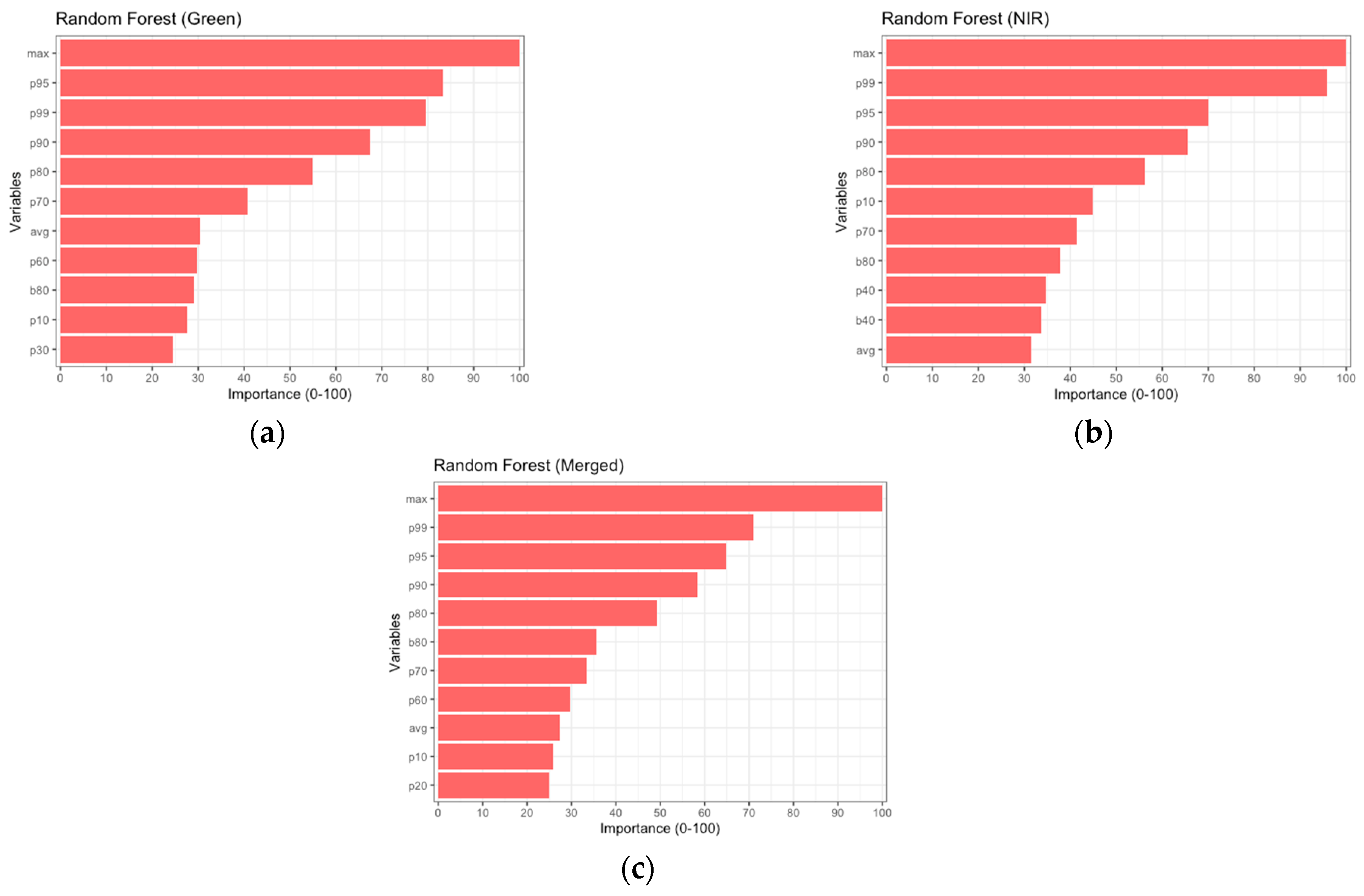
• The height-derived LiDAR metrics contributed to the accurate crown components biomass estimation, where they were the most important variables in the best-performing models, compared with the intensity-derived, none of which were selected.
• The metrics derived from the green point cloud provided the most accurate biomass predictions in all regression models and crown components.
• The use of monospectral point clouds (i.e., green and NIR) resulted in improved predictive accuracy compared with the multispectral, which can be attributed to the increased complexity of the merged point cloud.

Overall, it is evident that airborne LiDAR data could successfully contribute to quantifying carbon sequestration and biomass in complex structured forests, maintaining the ecosystem’s carbon balance. This study aids in improving crown biomass estimation in naturally regenerated ecosystems with a complex structure, where branches are among the most important surface fuel components. Given the limitations of the study described in Section 5, it would be interesting to examine the potential of LiDAR in crown components biomass estimation when employing an increased amount of destructive samples in order to validate the results. Further research could also focus on the use of spaceborne LiDAR systems to provide a cost-efficient approach for crown biomass estimation at large scales.

References

1. Allouis, T.; Durrieu, S.; Vega, C.; Couteron, P. Stem Volume and Above-Ground Biomass Estimation of Individual Pine Trees From LiDAR Data: Contribution of Full-Waveform Signals. IEEE J. Sel. Top. Appl. Earth Obs. Remote Sens. 2013, 6, 924–934. [Google Scholar] [CrossRef]
2. Kajimoto, T.; Matsuura, Y.; Sofronov, M.A.; Volokitina, A.V.; Mori, S.; Osawa, A.; Abaimov, A.P. Above- and Belowground Biomass and Net Primary Productivity of a Larix Gmelinii Stand near Tura, Central Siberia. Tree Physiol. 1999, 19, 815–822. [Google Scholar] [CrossRef]
3. Luo, S.; Wang, C.; Xi, X.; Pan, F.; Peng, D.; Zou, J.; Nie, S.; Qin, H. Fusion of Airborne LiDAR Data and Hyperspectral Imagery for Aboveground and Belowground Forest Biomass Estimation. Ecol. Indic. 2017, 73, 378–387. [Google Scholar] [CrossRef]
4. Duncanson, L.; Neuenschwander, A.; Hancock, S.; Thomas, N.; Fatoyinbo, T.; Simard, M.; Silva, C.A.; Armston, J.; Luthcke, S.B.; Hofton, M.; et al. Biomass Estimation from Simulated GEDI, ICESat-2 and NISAR across Environmental Gradients in Sonoma County, California. Remote Sens. Environ. 2020, 242, 111779. [Google Scholar] [CrossRef]
5. Zheng, Y.; Jia, W.; Wang, Q.; Huang, X. Deriving Individual-Tree Biomass from Effective Crown Data Generated by Terrestrial Laser Scanning. Remote Sens. 2019, 11, 2793. [Google Scholar] [CrossRef] [Green Version]
6. Hauglin, M.; Dibdiakova, J.; Gobakken, T.; Næsset, E. Estimating Single-Tree Branch Biomass of Norway Spruce by Airborne Laser Scanning. ISPRS J. Photogramm. Remote Sens. 2013, 79, 147–156. [Google Scholar] [CrossRef]
7. Tolunay, D. Carbon Concentrations of Tree Components, Forest Floor and Understorey in Young Pinus sylvestris Stands in North-Western Turkey. Scand. J. For. Res. 2009, 24, 394–402. [Google Scholar] [CrossRef]
8. García, M.; Riaño, D.; Chuvieco, E.; Danson, F.M. Estimating Biomass Carbon Stocks for a Mediterranean Forest in Central Spain Using LiDAR Height and Intensity Data. Remote Sens. Environ. 2010, 114, 816–830. [Google Scholar] [CrossRef]
9. Socha, J.; Wezyk, P. Allometric Equations for Estimating the Foliage Biomass of Scots Pine. Eur. J. For. Res. 2007, 126, 263–270. [Google Scholar] [CrossRef]
10. Dutcă, I.; Zianis, D.; Petrițan, I.C.; Bragă, C.I.; Ștefan, G.; Yuste, J.C.; Petrițan, A.M. Allometric Biomass Models for European Beech and Silver Fir: Testing Approaches to Minimize the Demand for Site-Specific Biomass Observations. Forests 2020, 11, 1136. [Google Scholar] [CrossRef]
11. Torre-Tojal, L.; Bastarrika, A.; Boyano, A.; Lopez-Guede, J.M.; Graña, M. Above-Ground Biomass Estimation from LiDAR Data Using Random Forest Algorithms. J. Comput. Sci. 2022, 58, 101517. [Google Scholar] [CrossRef]
12. Wang, X.; Jiao, H. Spatial Scaling of Forest Aboveground Biomass Using Multi-Source Remote Sensing Data. IEEE Access 2020, 8, 178870–178885. [Google Scholar] [CrossRef]
13. Roy, P.S.; Ravan, S.A. Biomass Estimation Using Satellite Remote Sensing Data—An Investigation on Possible Approaches for Natural Forest. J. Biosci. 1996, 21, 535–561. [Google Scholar] [CrossRef]
14. Muukkonen, P.; Heiskanen, J. Biomass Estimation over a Large Area Based on Standwise Forest Inventory Data and ASTER and MODIS Satellite Data: A Possibility to Verify Carbon Inventories. Remote Sens. Environ. 2007, 107, 617–624. [Google Scholar] [CrossRef]
15. Sousa, A.M.O.; Gonçalves, A.C.; Mesquita, P.; Marques da Silva, J.R. Biomass Estimation with High Resolution Satellite Images: A Case Study of Quercus rotundifolia. ISPRS J. Photogramm. Remote Sens. 2015, 101, 69–79. [Google Scholar] [CrossRef] [Green Version]
16. Chrysafis, I.; Mallinis, G.; Gitas, I.; Tsakiri-Strati, M. Estimating Mediterranean Forest Parameters Using Multi Seasonal Landsat 8 OLI Imagery and an Ensemble Learning Method. Remote Sens. Environ. 2017, 199, 154–166. [Google Scholar] [CrossRef]
17. Solberg, S. Estimating Spruce and Pine Biomass with Interferometric X-Band SAR. Remote Sens. Environ. 2010, 114, 2353–2360. [Google Scholar] [CrossRef]
18. Schlund, M.; Davidson, M.W.J. Aboveground Forest Biomass Estimation Combining L- and P-Band SAR Acquisitions. Remote Sens. 2018, 10, 1151. [Google Scholar] [CrossRef] [Green Version]
19. Domingues, G.F.; Soares, V.P.; Leite, H.G.; Ferraz, A.S.; Ribeiro, C.A.A.S.; Lorenzon, A.S.; Marcatti, G.E.; Teixeira, T.R.; de Castro, N.L.M.; Mota, P.H.S.; et al. Artificial Neural Networks on Integrated Multispectral and SAR Data for High-Performance Prediction of Eucalyptus Biomass. Comput. Electron. Agric. 2020, 168, 105089. [Google Scholar] [CrossRef]
20. Gleason, C.J.; Im, J. Forest Biomass Estimation from Airborne LiDAR Data Using Machine Learning Approaches. Remote Sens. Environ. 2012, 125, 80–91. [Google Scholar] [CrossRef]
21. Duncanson, L.; Kellner, J.R.; Armston, J.; Dubayah, R.; Minor, D.M.; Hancock, S.; Healey, S.P.; Patterson, P.L.; Saarela, S.; Marselis, S.; et al. Aboveground Biomass Density Models for NASA’s Global Ecosystem Dynamics Investigation (GEDI) Lidar Mission. Remote Sens. Environ. 2022, 270, 112845. [Google Scholar] [CrossRef]
22. Wang, Q.; Pang, Y.; Chen, D.; Liang, X.; Lu, J. Lidar Biomass Index: A Novel Solution for Tree-Level Biomass Estimation Using 3D Crown Information. For. Ecol. Manag. 2021, 499, 119542. [Google Scholar] [CrossRef]
23. Ni-Meister, W.; Rojas, A.; Lee, S. Direct Use of Large-Footprint Lidar Waveforms to Estimate Aboveground Biomass. Remote Sens. Environ. 2022, 280, 113147. [Google Scholar] [CrossRef]
24. Stovall, A.E.L.; Anderson-Teixeira, K.J.; Shugart, H.H. Assessing Terrestrial Laser Scanning for Developing Non-Destructive Biomass Allometry. For. Ecol. Manag. 2018, 427, 217–229. [Google Scholar] [CrossRef]
25. Næsset, E.; Gobakken, T.; Solberg, S.; Gregoire, T.G.; Nelson, R.; Ståhl, G.; Weydahl, D. Model-Assisted Regional Forest Bi-omass Estimation Using LiDAR and InSAR as Auxiliary Data: A Case Study from a Boreal Forest Area. Remote Sens. Environ. 2011, 115, 3599–3614. [Google Scholar] [CrossRef]
26. Ghosh, S.M. Aboveground Biomass Estimation Using Multi-Sensor Data Synergy and Machine Learning Algorithms in a Dense Tropical Forest. Appl. Geogr. 2018, 96, 29–40. [Google Scholar] [CrossRef]
27. He, Q.-S.; Cao, C.-X.; Chen, E.-X.; Sun, G.-Q.; Ling, F.-L.; Pang, Y.; Zhang, H.; Ni, W.-J.; Xu, M.; Li, Z.-Y.; et al. Forest Stand Biomass Estimation Using ALOS PALSAR Data Based on LiDAR-Derived Prior Knowledge in the Qilian Mountain, Western China. Int. J. Remote Sens. 2012, 33, 710–729. [Google Scholar] [CrossRef]
28. Li, Y.; Li, M.; Li, C.; Liu, Z. Forest Aboveground Biomass Estimation Using Landsat 8 and Sentinel-1A Data with Machine Learning Algorithms. Sci. Rep. 2020, 10, 9952. [Google Scholar] [CrossRef]
29. Theofanous, N.; Chrysafis, I.; Mallinis, G.; Domakinis, C.; Verde, N.; Siahalou, S. Aboveground Biomass Estimation in Short Rotation Forest Plantations in Northern Greece Using ESA’s Sentinel Medium-High Resolution Multispectral and Radar Imaging Missions. Forests 2021, 12, 902. [Google Scholar] [CrossRef]
30. Sinha, S.; Jeganathan, C.; Sharma, L.K.; Nathawat, M.S. A Review of Radar Remote Sensing for Biomass Estimation. Int. J. Environ. Sci. Technol. 2015, 12, 1779–1792. [Google Scholar] [CrossRef] [Green Version]
31. Jiang, X.; Li, G.; Lu, D.; Chen, E.; Wei, X. Stratification-Based Forest Aboveground Biomass Estimation in a Subtropical Region Using Airborne Lidar Data. Remote Sens. 2020, 12, 1101. [Google Scholar] [CrossRef] [Green Version]
32. Ma, Q.; Su, Y.; Luo, L.; Li, L.; Kelly, M.; Guo, Q. Evaluating the Uncertainty of Landsat-Derived Vegetation Indices in Quantifying Forest Fuel Treatments Using Bi-Temporal LiDAR Data. Ecol. Indic. 2018, 95, 298–310. [Google Scholar] [CrossRef] [Green Version]
33. Francini, S.; D’Amico, G.; Vangi, E.; Borghi, C.; Chirici, G. Integrating GEDI and Landsat: Spaceborne Lidar and Four Decades of Optical Imagery for the Analysis of Forest Disturbances and Biomass Changes in Italy. Sensors 2022, 22, 2015. [Google Scholar] [CrossRef] [PubMed]
34. Maltamo, M.; Eerikäinen, K.; Packalén, P.; Hyyppä, J. Estimation of Stem Volume Using Laser Scanning-Based Canopy Height Metrics. Forestry 2006, 79, 217–229. [Google Scholar] [CrossRef] [Green Version]
35. Yu, X.; Hyyppä, J.; Vastaranta, M.; Holopainen, M.; Viitala, R. Predicting Individual Tree Attributes from Airborne Laser Point Clouds Based on the Random Forests Technique. ISPRS J. Photogramm. Remote Sens. 2011, 66, 28–37. [Google Scholar] [CrossRef]
36. Packalen, P.; Maltamo, M. Predicting the Plot Volume by Tree Species Using Airborne Laser Scanning and Aerial Photographs. For. Sci. 2006, 52, 611–622. [Google Scholar]
37. Stefanidou, A.; Gitas, I.Z.; Korhonen, L.; Georgopoulos, N.; Stavrakoudis, D. Multispectral LiDAR-Based Estimation of Surface Fuel Load in a Dense Coniferous Forest. Remote Sens. 2020, 12, 3333. [Google Scholar] [CrossRef]
38. Andersen, H.-E.; McGaughey, R.J.; Reutebuch, S.E. Estimating Forest Canopy Fuel Parameters Using LIDAR Data. Remote Sens. Environ. 2005, 94, 441–449. [Google Scholar] [CrossRef]
39. Popescu, S.C.; Zhao, K. A Voxel-Based Lidar Method for Estimating Crown Base Height for Deciduous and Pine Trees. Remote Sens. Environ. 2008, 112, 767–781. [Google Scholar] [CrossRef]
40. Kelly, M.; Su, Y.; Di Tommaso, S.; Fry, D.; Collins, B.; Stephens, S.; Guo, Q. Impact of Error in Lidar-Derived Canopy Height and Canopy Base Height on Modeled Wildfire Behavior in the Sierra Nevada, California, USA. Remote Sens. 2017, 10, 10. [Google Scholar] [CrossRef] [Green Version]
41. Greaves, H.E.; Vierling, L.A.; Eitel, J.U.H.; Boelman, N.T.; Magney, T.S.; Prager, C.M.; Griffin, K.L. Estimating Aboveground Biomass and Leaf Area of Low-Stature Arctic Shrubs with Terrestrial LiDAR. Remote Sens. Environ. 2015, 164, 26–35. [Google Scholar] [CrossRef]
42. Kamoske, A.G.; Dahlin, K.M.; Stark, S.C.; Serbin, S.P. Leaf Area Density from Airborne LiDAR: Comparing Sensors and Resolutions in a Temperate Broadleaf Forest Ecosystem. For. Ecol. Manag. 2019, 433, 364–375. [Google Scholar] [CrossRef]
43. Beets, P.N.; Reutebuch, S.; Kimberley, M.O.; Oliver, G.R.; Pearce, S.H.; McGaughey, R.J. Leaf Area Index, Biomass Carbon and Growth Rate of Radiata Pine Genetic Types and Relationships with LiDAR. Forests 2011, 2, 637–659. [Google Scholar] [CrossRef] [Green Version]
44. Pope, G.; Treitz, P. Leaf Area Index (LAI) Estimation in Boreal Mixedwood Forest of Ontario, Canada Using Light Detection and Ranging (LiDAR) and WorldView-2 Imagery. Remote Sens. 2013, 5, 5040–5063. [Google Scholar] [CrossRef] [Green Version]
45. Georgopoulos, N.; Gitas, I.Z.; Stefanidou, A.; Korhonen, L.; Stavrakoudis, D. Estimation of Individual Tree Stem Biomass in an Uneven-Aged Structured Coniferous Forest Using Multispectral LiDAR Data. Remote Sens. 2021, 13, 4827. [Google Scholar] [CrossRef]
46. Dalponte, M.; Frizzera, L.; Ørka, H.O.; Gobakken, T.; Næsset, E.; Gianelle, D. Predicting Stem Diameters and Aboveground Biomass of Individual Trees Using Remote Sensing Data. Ecol. Indic. 2018, 85, 367–376. [Google Scholar] [CrossRef]
47. Dalponte, M.; Coomes, D.A. Tree-centric Mapping of Forest Carbon Density from Airborne Laser Scanning and Hyperspectral Data. Methods Ecol. Evol. 2016, 7, 1236–1245. [Google Scholar] [CrossRef] [Green Version]
48. Speak, A.; Escobedo, F.J.; Russo, A.; Zerbe, S. Total Urban Tree Carbon Storage and Waste Management Emissions Estimated Using a Combination of LiDAR, Field Measurements and an End-of-Life Wood Approach. J. Clean. Prod. 2020, 256, 120420. [Google Scholar] [CrossRef]
49. Coomes, D.A.; Dalponte, M.; Jucker, T.; Asner, G.P.; Banin, L.F.; Burslem, D.F.R.P.; Lewis, S.L.; Nilus, R.; Phillips, O.L.; Phua, M.-H.; et al. Area-Based vs. Tree-Centric Approaches to Mapping Forest Carbon in Southeast Asian Forests from Airborne Laser Scanning Data. Remote Sens. Environ. 2017, 194, 77–88. [Google Scholar] [CrossRef] [Green Version]
50. Yu, X.; Hyyppä, J.; Holopainen, M.; Vastaranta, M. Comparison of Area-Based and Individual Tree-Based Methods for Pre-dicting Plot-Level Forest Attributes. Remote Sens. 2010, 2, 1481–1495. [Google Scholar] [CrossRef] [Green Version]
51. Popescu, S.C. Estimating Biomass of Individual Pine Trees Using Airborne Lidar. Biomass Bioenergy 2007, 31, 646–655. [Google Scholar] [CrossRef]
52. Li, C.; Yu, Z.; Wang, S.; Wu, F.; Wen, K.; Qi, J.; Huang, H. Crown Structure Metrics to Generalize Aboveground Biomass Estimation Model Using Airborne Laser Scanning Data in National Park of Hainan Tropical Rainforest, China. Forests 2022, 13, 1142. [Google Scholar] [CrossRef]
53. Ene, L.T. Assessing the Accuracy of Regional LiDAR-Based Biomass Estimation Using a Simulation Approach. Remote Sens. Environ. 2012, 123, 579–592. [Google Scholar] [CrossRef]
54. Rex, F.E.; Silva, C.A.; Dalla Corte, A.P.; Klauberg, C.; Mohan, M.; Cardil, A.; da Silva, V.S.; de Almeida, D.R.A.; Garcia, M.; Broadbent, E.N.; et al. Comparison of Statistical Modelling Approaches for Estimating Tropical Forest Aboveground Biomass Stock and Reporting Their Changes in Low-Intensity Logging Areas Using Multi-Temporal LiDAR Data. Remote Sens. 2020, 12, 1498. [Google Scholar] [CrossRef]
55. Latifi, H.; Nothdurft, A.; Koch, B. Non-Parametric Prediction and Mapping of Standing Timber Volume and Biomass in a Temperate Forest: Application of Multiple Optical/LiDAR-Derived Predictors. Forestry 2010, 83, 395–407. [Google Scholar] [CrossRef] [Green Version]
56. Sun, X.; Li, G.; Wang, M.; Fan, Z. Analyzing the Uncertainty of Estimating Forest Aboveground Biomass Using Optical Imagery and Spaceborne LiDAR. Remote Sens. 2019, 11, 722. [Google Scholar] [CrossRef] [Green Version]
57. Fehrmann, L.; Lehtonen, A.; Kleinn, C.; Tomppo, E. Comparison of Linear and Mixed-Effect Regression Models and a k-Nearest Neighbour Approach for Estimation of Single-Tree Biomass. Can. J. For. Res. 2008, 38, 1–9. [Google Scholar] [CrossRef]
58. Kankare, V.; Räty, M.; Yu, X.; Holopainen, M.; Vastaranta, M.; Kantola, T.; Hyyppä, J.; Hyyppä, H.; Alho, P.; Viitala, R. Single Tree Biomass Modelling Using Airborne Laser Scanning. ISPRS J. Photogramm. Remote Sens. 2013, 85, 66–73. [Google Scholar] [CrossRef]
59. Zhang, Y.; Borders, B.E.; Will, R.E. A Model for Foliage and Branch Biomass Prediction for Intensively Managed Fast Grow-ing Loblolly Pine. For. Sci. 2004, 50, 65–80. [Google Scholar]
60. Korhonen, L.; Vauhkonen, J.; Virolainen, A.; Hovi, A.; Korpela, I. Estimation of Tree Crown Volume from Airborne Lidar Data Using Computational Geometry. Int. J. Remote Sens. 2013, 34, 7236–7248. [Google Scholar] [CrossRef]
61. Hauglin, M.; Gobakken, T.; Astrup, R.; Ene, L. Estimating Single-Tree Crown Biomass of Norway Spruce by Airborne Laser Scanning: A Comparison of Methods with and without the Use of Terrestrial Laser Scanning to Obtain the Ground Reference Data. Forests 2014, 5, 384–403. [Google Scholar] [CrossRef]
62. Cao, L.; Coops, N.; Innes, J.; Dai, J.; She, G. Mapping Above- and Below-Ground Biomass Components in Subtropical Forests Using Small-Footprint LiDAR. Forests 2014, 5, 1356–1373. [Google Scholar] [CrossRef] [Green Version]
63. Li, W.; Niu, Z.; Gao, S.; Huang, N.; Chen, H. Correlating the Horizontal and Vertical Distribution of LiDAR Point Clouds with Components of Biomass in a Picea Crassifolia Forest. Forests 2014, 5, 1910–1930. [Google Scholar] [CrossRef] [Green Version]
64. Wallace, A.; Nichol, C.; Woodhouse, I. Recovery of Forest Canopy Parameters by Inversion of Multispectral LiDAR Data. Remote Sens. 2012, 4, 509–531. [Google Scholar] [CrossRef] [Green Version]
65. Zhang, Z.; Li, T.; Tang, X.; Lei, X.; Peng, Y. Introducing Improved Transformer to Land Cover Classification Using Multispectral LiDAR Point Clouds. Remote Sens. 2022, 14, 3808. [Google Scholar] [CrossRef]
66. Kukkonen, M.; Maltamo, M.; Korhonen, L.; Packalen, P. Multispectral Airborne LiDAR Data in the Prediction of Boreal Tree Species Composition. IEEE Trans. Geosci. Remote Sens. 2019, 57, 3462–3471. [Google Scholar] [CrossRef]
67. Maltamo, M.; Räty, J.; Korhonen, L.; Kotivuori, E.; Kukkonen, M.; Peltola, H.; Kangas, J.; Packalen, P. Prediction of Forest Canopy Fuel Parameters in Managed Boreal Forests Using Multispectral and Unispectral Airborne Laser Scanning Data and Aerial Images. Eur. J. Remote Sens. 2020, 53, 245–257. [Google Scholar] [CrossRef]
68. Dalponte, M.; Ene, L.; Gobakken, T.; Næsset, E.; Gianelle, D. Predicting Selected Forest Stand Characteristics with Multispectral ALS Data. Remote Sens. 2018, 10, 586. [Google Scholar] [CrossRef] [Green Version]
69. Dai, W.; Yang, B.; Dong, Z.; Shaker, A. A New Method for 3D Individual Tree Extraction Using Multispectral Airborne LiDAR Point Clouds. ISPRS J. Photogramm. Remote Sens. 2018, 144, 400–411. [Google Scholar] [CrossRef]
70. Harrison, D.; Hunter, M.C.; Lewis, A.C.; Seakins, P.W.; Nunes, T.V.; Pio, C.A. Isoprene and Monoterpene Emission from the Coniferous Species Abies Borisii-Regis—Implications for Regional Air Chemistry in Greece. Atmos. Environ. 2001, 35, 4687–4698. [Google Scholar] [CrossRef]
71. Dietrich, R.; Anand, M. Trees Do Not Always Act Their Age: Size-Deterministic Tree Ring Standardization for Long-Term Trend Estimation in Shade-Tolerant Trees. Biogeosciences 2019, 16, 4815–4827. [Google Scholar] [CrossRef] [Green Version]
72. Kwak, D.-A.; Lee, W.-K.; Cho, H.-K.; Lee, S.-H.; Son, Y.; Kafatos, M.; Kim, S.-R. Estimating Stem Volume and Biomass of Pinus koraiensis Using LiDAR Data. J. Plant Res. 2010, 123, 421–432. [Google Scholar] [CrossRef] [PubMed]
73. Zianis, D.; Xanthopoulos, G.; Kalabokidis, K.; Kazakis, G.; Ghosn, D.; Roussou, O. Allometric Equations for Aboveground Biomass Estimation by Size Class for Pinus brutia Ten. Trees Growing in North and South Aegean Islands, Greece. Eur. J. For. Res. 2011, 130, 145–160. [Google Scholar] [CrossRef]
74. R Core Team. R: A Language and Environment for Statistical Computing; R Foundation for Statistical Computing: Vienna, Austria, 2017. [Google Scholar]
75. Roussel, J.-R.; Auty, D.; Coops, N.C.; Tompalski, P.; Goodbody, T.R.H.; Meador, A.S.; Bourdon, J.-F.; de Boissieu, F.; Achim, A. LidR: An R Package for Analysis of Airborne Laser Scanning (ALS) Data. Remote Sens. Environ. 2020, 251, 112061. [Google Scholar] [CrossRef]
76. Gatziolis, D. Dynamic Range-Based Intensity Normalization for Airborne, Discrete Return Lidar Data of Forest Canopies. Photogramm. Eng. Remote Sens. 2011, 77, 251–259. [Google Scholar] [CrossRef]
77. Yoga, S.; Bégin, J.; St-Onge, B.; Gatziolis, D. Lidar and Multispectral Imagery Classifications of Balsam Fir Tree Status for Accurate Predictions of Merchantable Volume. Forests 2017, 8, 253. [Google Scholar] [CrossRef] [Green Version]
78. Korpela, I.; Hovi, A.; Morsdorf, F. Understory Trees in Airborne LiDAR Data—Selective Mapping Due to Transmission Losses and Echo-Triggering Mechanisms. Remote Sens. Environ. 2012, 119, 92–104. [Google Scholar] [CrossRef]
79. Carrilho, A.C.; Galo, M.; Santos, R.C. Statistical Outlier Detection Method for Airborne Lidar Data. Int. Arch. Photogramm. Remote Sens. Spat. Inf. Sci. 2018, XLII–1, 87–92. [Google Scholar] [CrossRef] [Green Version]
80. Zhang, W.; Qi, J.; Wan, P.; Wang, H.; Xie, D.; Wang, X.; Yan, G. An Easy-to-Use Airborne LiDAR Data Filtering Method Based on Cloth Simulation. Remote Sens. 2016, 8, 501. [Google Scholar] [CrossRef]
81. Khosravipour, A.; Skidmore, A.K.; Isenburg, M.; Wang, T.; Hussin, Y.A. Generating Pit-Free Canopy Height Models from Airborne Lidar. Photogramm. Eng. Remote Sens. 2014, 80, 863–872. [Google Scholar] [CrossRef]
82. Kodors, S. Point Distribution as True Quality of LiDAR Point Cloud. Balt. J. Mod. Comput. 2017, 5, 362–378. [Google Scholar] [CrossRef]
83. Silva, C.A.; Hudak, A.T.; Vierling, L.A.; Loudermilk, E.L.; O’Brien, J.J.; Hiers, J.K.; Jack, S.B.; Gonzalez-Benecke, C.; Lee, H.; Falkowski, M.J.; et al. Imputation of Individual Longleaf Pine (Pinus palustris Mill.) Tree Attributes from Field and LiDAR Data. Can. J. Remote Sens. 2016, 42, 554–573. [Google Scholar] [CrossRef]
84. Duan, Z.; Zhao, D.; Zeng, Y.; Zhao, Y.; Wu, B.; Zhu, J. Assessing and Correcting Topographic Effects on Forest Canopy Height Retrieval Using Airborne LiDAR Data. Sensors 2015, 15, 12133–12155. [Google Scholar] [CrossRef]
85. Eysn, L.; Hollaus, M.; Lindberg, E.; Berger, F.; Monnet, J.-M.; Dalponte, M.; Kobal, M.; Pellegrini, M.; Lingua, E.; Mongus, D.; et al. A Benchmark of Lidar-Based Single Tree Detection Methods Using Heterogeneous Forest Data from the Alpine Space. Forests 2015, 6, 1721–1747. [Google Scholar] [CrossRef] [Green Version]
86. Goldbergs, G.; Levick, S.R.; Lawes, M.; Edwards, A. Hierarchical Integration of Individual Tree and Area-Based Approaches for Savanna Biomass Uncertainty Estimation from Airborne LiDAR. Remote Sens. Environ. 2018, 205, 141–150. [Google Scholar] [CrossRef]
87. Xiang, W.; Li, L.; Ouyang, S.; Xiao, W.; Zeng, L.; Chen, L.; Lei, P.; Deng, X.; Zeng, Y.; Fang, J.; et al. Effects of Stand Age on Tree Biomass Partitioning and Allometric Equations in Chinese Fir (Cunninghamia lanceolata) Plantations. Eur. J. For. Res. 2021, 140, 317–332. [Google Scholar] [CrossRef]
88. Zianis, D.; Mencuccini, M. Aboveground Biomass Relationships for Beech (Fagus moesiaca Cz.) Trees in Vermio Mountain, Northern Greece, and Generalised Equations for Fagus sp. Ann. For. Sci. 2003, 60, 439–448. [Google Scholar] [CrossRef] [Green Version]
89. Martin, F.S.; Navarro-Cerrillo, R.M.; Mulia, R.; van Noordwijk, M. Allometric Equations Based on a Fractal Branching Model for Estimating Aboveground Biomass of Four Native Tree Species in the Philippines. Agroforest Syst. 2010, 78, 193–202. [Google Scholar] [CrossRef]
90. Tziaferidis, S.; Spyroglou, G.; Fotelli, M.; Radoglou, K. Allometric Models for the Estimation of Foliage Area and Biomass from Stem Metrics in Black Locust. iForest 2022, 15, 281–288. [Google Scholar] [CrossRef]
91. Wainer, J.; Cawley, G. Nested Cross-Validation When Selecting Classifiers Is Overzealous for Most Practical Applications. Expert Syst. Appl. 2021, 182, 115222. [Google Scholar] [CrossRef]
92. Cade, B.S. Model Averaging and Muddled Multimodel Inferences. Ecology 2015, 96, 2370–2382. [Google Scholar] [CrossRef] [Green Version]
93. Tibshirani, S.; Friedman, H. The Elements of Statistical Learning; Springer Science & Business Media: Berlin/Heidelberg, Germany, 2001. [Google Scholar]
94. Silveira, E.M.O.; Silva, S.H.G.; Acerbi-Junior, F.W.; Carvalho, M.C.; Carvalho, L.M.T.; Scolforo, J.R.S.; Wulder, M.A. Object-Based Random Forest Modelling of Aboveground Forest Biomass Outperforms a Pixel-Based Approach in a Heterogeneous and Mountain Tropical Environment. Int. J. Appl. Earth Obs. Geoinf. 2019, 78, 175–188. [Google Scholar]
95. Strobl, C.; Malley, J.; Tutz, G. An Introduction to Recursive Partitioning: Rationale, Application, and Characteristics of Classification and Regression Trees, Bagging, and Random Forests. Psychol. Methods 2009, 14, 323–348. [Google Scholar] [CrossRef] [PubMed] [Green Version]
96. Cortes, C.; Vapnik, V. Support-Vector Networks. Mach. Learn. 1995, 20, 273–297. [Google Scholar] [CrossRef]
97. Corte, A.P.D.; Souza, D.V.; Rex, F.E.; Sanquetta, C.R.; Mohan, M.; Silva, C.A.; Zambrano, A.M.A.; Prata, G.; Alves de Almeida, D.R.; Trautenmüller, J.W.; et al. Forest Inventory with High-Density UAV-Lidar: Machine Learning Approaches for Predicting Individual Tree Attributes. Comput. Electron. Agric. 2020, 179, 105815. [Google Scholar] [CrossRef]
98. Diamantopoulou, M.J.; Özçelik, R.; Yavuz, H. Tree-Bark Volume Prediction via Machine Learning: A Case Study Based on Black Alder’s Tree-Bark Production. Comput. Electron. Agric. 2018, 151, 431–440. [Google Scholar] [CrossRef]
99. Marabel, M.; Alvarez-Taboada, F. Spectroscopic Determination of Aboveground Biomass in Grasslands Using Spectral Transformations, Support Vector Machine and Partial Least Squares Regression. Sensors 2013, 13, 10027–10051. [Google Scholar] [CrossRef] [Green Version]
100. Wang, J. An Intuitive Tutorial to Gaussian Processes Regression. arXiv 2021, arXiv:2009.10862. [Google Scholar]
101. Bousquet, O.; von Luxburg, U.; Rätsch, G. (Eds.) Advanced Lectures on Machine Learning: ML Summer Schools 2003, Canberra, Australia, 2–14 February 2003, Tübingen, Germany, 4–16 August 2003, Revised Lectures; Lecture Notes in Computer Science, Lecture Notes in Artificial Intelligence; Springer: Berlin/Heidelberg, Germany; New York, NY, USA, 2004; ISBN 978-3-540-23122-6. [Google Scholar]
102. Pham, T.D.; Le, N.N.; Ha, N.T.; Nguyen, L.V.; Xia, J.; Yokoya, N.; To, T.T.; Trinh, H.X.; Kieu, L.Q.; Takeuchi, W. Estimating Mangrove Above-Ground Biomass Using Extreme Gradient Boosting Decision Trees Algorithm with Fused Sentinel-2 and ALOS-2 PALSAR-2 Data in Can Gio Biosphere Reserve, Vietnam. Remote Sens. 2020, 12, 777. [Google Scholar] [CrossRef] [Green Version]
103. Perez-Cruz, F.; Van Vaerenbergh, S.; Murillo-Fuentes, J.J.; Lazaro-Gredilla, M.; Santamaria, I. Gaussian Processes for Nonlinear Signal Processing: An Overview of Recent Advances. IEEE Signal Process. Mag. 2013, 30, 40–50. [Google Scholar] [CrossRef] [Green Version]
104. Peichl, M.; Arain, M.A. Allometry and Partitioning of Above- and Belowground Tree Biomass in an Age-Sequence of White Pine Forests. For. Ecol. Manag. 2007, 253, 68–80. [Google Scholar] [CrossRef]
105. Kuo, K.; Itakura, K.; Hosoi, F. Leaf Segmentation Based on K-Means Algorithm to Obtain Leaf Angle Distribution Using Terrestrial LiDAR. Remote Sens. 2019, 11, 2536. [Google Scholar] [CrossRef] [Green Version]
106. Naik, P.; Dalponte, M.; Bruzzone, L. Prediction of Forest Aboveground Biomass Using Multitemporal Multispectral Remote Sensing Data. Remote Sens. 2021, 13, 1282. [Google Scholar] [CrossRef]
107. He, Q.; Chen, E.; An, R.; Li, Y. Above-Ground Biomass and Biomass Components Estimation Using LiDAR Data in a Coniferous Forest. Forests 2013, 4, 984–1002. [Google Scholar] [CrossRef] [Green Version]
108. Hopkinson, C.; Chasmer, L.; Gynan, C.; Mahoney, C.; Sitar, M. Multisensor and Multispectral LiDAR Characterization and Classification of a Forest Environment. Can. J. Remote Sens. 2016, 42, 501–520. [Google Scholar] [CrossRef]
Figure 1. Vegetation map of the study area, including the sampling plots and road network.
Remotesensing 15 02919 g001
Figure 2. Canopy height model of Pertouli University Forest generated from ALS data showing the sampled trees: (af) areas employed for non-destructive sampling (i.e., measurement of DBH, H, canopy base height and crown radii for crown biomass estimation using allometric equations); (g) specific trees and area of interest for destructive sampling.
Remotesensing 15 02919 g002
Figure 3. Flowchart of the workflow for the single-tree dead branches, needles and branch biomass (DB, NB, and BB, respectively) estimations using destructive sampling and multispectral ALS data in a multilayered fir forest.
Remotesensing 15 02919 g003
Figure 4. Scatterplots of the observed versus the predicted dead branches biomass (DB) for the best performing algorithm in each point cloud, based on 46 testing samples. The blue line represents the fitted line, and the red line represents the 1:1 line.
Remotesensing 15 02919 g004
Figure 5. Demonstration of the relative importance (ac) of the predictors for the best-performing algorithm for DB estimation in each point cloud based on the random forest algorithm.
Remotesensing 15 02919 g005
Figure 6. Scatterplots of the observed versus the predicted needles biomass (NB) for the best performing algorithm in each point cloud, based on 46 training samples. The blue line represents the fitted line, and the red line represents the 1:1 line.
Remotesensing 15 02919 g006
Figure 7. Demonstration of the relative importance (ac) of the predictors for the best-performing algorithm for NB estimation in each point cloud based on the random forest algorithm.
Remotesensing 15 02919 g007
Figure 8. Scatterplots of the observed versus predicted branches biomass (BB) for the best-performing algorithm in each point cloud based on 46 testing samples. The blue line represents the fitted line and the red line represents the 1:1 line.
Remotesensing 15 02919 g008
Figure 9. Demonstration of the relative importance (ac) of the predictors for the best-performing algorithm for BB estimation in each point cloud based on the random forest algorithm.
Remotesensing 15 02919 g009