Article

Multi-Temporal Remote Sensing Inversion of Evapotranspiration in the Lower Yangtze River Based on Landsat 8 Remote Sensing Data and Analysis of Driving Factors

1
College of Agricultural Science and Engineering, Hohai University, Nanjing 211100, China
2
College of Water Resources and Hydropower, Xi’an University of Technology, Xi’an 710048, China
3
School of Agricultural Engineering, Jiangsu University, Zhenjiang 212013, China
*
Author to whom correspondence should be addressed.
Remote Sens. 2023, 15(11), 2887; https://doi.org/10.3390/rs15112887
Submission received: 24 April 2023 / Revised: 24 May 2023 / Accepted: 31 May 2023 / Published: 1 June 2023
(This article belongs to the Special Issue Advances in the Remote Sensing of Terrestrial Evaporation II)

Abstract

:
Analysis of the spatial and temporal variation patterns of surface evapotranspiration is important for understanding global climate change, promoting scientific deployment of regional water resources, and improving crop yield and water productivity. Based on Landsat 8 OIL_TIRS data and remote sensing image data of the lower Yangtze River urban cluster for the same period of 2016–2021, combined with soil and meteorological data of the study area, this paper constructed a multiple linear regression (MLR) model and an extreme learning machine (ELM) inversion model with evapotranspiration as the target and, based on the model inversion, quantitatively and qualitatively analyzed the spatial and temporal variability in surface evapotranspiration in the study area in the past six years. The results show that both models based on feature factors and spectral indices obtained a good inversion accuracy, with the fusion of feature factors effectively improving the inversion ability of the model for ET. The best model for ET in 2016, 2017, and 2021 was MLR, with an R2 greater than 0.8; the best model for ET in 2018–2019 was ELM, with an R2 of 0.83 and 0.62, respectively. The inter-annual ET in the study area showed a “double-peak” dynamic variation, with peaks in 2018 and 2020; the intra-annual ET showed a single-peak cycle, with peaks in July–August. Seasonal differences were obvious, and spatially high-ET areas were mainly found in rural areas north of the Yangtze River and central and western China where agricultural land is concentrated. The net solar radiation, soil heat flux, soil temperature and humidity, and fractional vegetation cover all had significant positive effects on ET, with correlation coefficients ranging from 0.39 to 0.94. This study can provide methodological and scientific support for the quantitative and qualitative estimation of regional ET.

1. Introduction

Evapotranspiration (ET) is the process by which surface water is transferred to the atmosphere, including evaporation of water vapor captured from water bodies, soils, and vegetation surfaces, and transpiration by plants [1]. Evapotranspiration is a major component of the global water cycle and is a key link between terrestrial water, carbon, and surface energy exchange, with strong links to agriculture, hydrology, meteorology, and ecology [2]. Accurate estimates of evapotranspiration are important for understanding global climate change, ecological issues, the water cycle, and hydrological processes, as well as for improving water use efficiency, crop yields, and water productivity [3,4,5].
The conventional estimation method for ET is to analyze meteorological data through the information obtained from meteorological stations and ground flux monitoring stations in different areas [6], but the above estimation method is only a point estimate of a single station, which is not suitable for large-scale and multi-temporal ET estimation, and more manpower and material resources are required to install evapotranspiration systems in a large area [7]. With the rapid development of remote sensing technology, remote sensing technology has overcome the shortage of spatial variability and multi-temporal phases based on single-site observations due to its short detection period, strong presentability, and its ability to observe simultaneously over a large area [8,9]. Since the 1980s, with the extensive use of polar-orbiting meteorological satellites, the efficient space measurement capability has provided a cost-effective method for monitoring ET on a large scale [10]. At present, many scholars have conducted several studies on the simulation and inversion of large-scale evapotranspiration using Landsat series satellites and MODIS series satellites [11,12].
The inversion methods for evapotranspiration remote sensing can be classified into process-driven physical inversion methods and data-driven inversion methods according to the principal mechanism [13]. Physical inversion methods include energy balance residual methods and methods based on Penman–Monteith or Priestley–Taylor formulas. Wang [14] et al. studied ET for different land use types based on meteorological data of the Sanmenxia reservoir watershed in China using Landsat 8 OIL_TIRS remote sensing images as an example. Gao [15] et al. studied ET for different land use types based on MODIS data and Sentinel-2 data, using the SEBAL model and the Penman–Monteith equation to estimate the ET of field crops. Yang [16] et al. successfully simulated the spatial distribution of ET in the Haihe Plain in northern China by establishing an irrigation application (IA) estimation model and an EI calculation model based on remote sensing data. Liu et al. [17] used data from meteorological stations in Sichuan Province, China, and MODIS data products to validate the MODIS-predicted evapotranspiration through the estimated actual evapotranspiration. The process-driven approach addresses the theory of plant photosynthesis, canopy respiration, and soil evapotranspiration in the ET production mechanism, using simplified ecosystem processes and components to form a model structure for simulating ecosystem carbon and water energy exchange [18,19]. However, the heterogeneity of regional surfaces, the complexity of parameter selection, and the cumulative error of different models can lead to process-driven models being more complex in estimating ET at large scales and in multiple time phases, and the accuracy of the results is limited by the quality of the input data, making it difficult to obtain the desired regional estimation accuracy.
Data-driven inversion methods include empirical regression methods, machine learning methods, and data fusion methods. Liu et al. [20] used global eddy covariance flux point data to compare the applicability of different machine learning models for the remote sensing estimation of farmland ET, with good results. Han et al. [21] studied the relationship between drought and precipitation, temperature, vegetation, and evapotranspiration using random forest (RF) and, by introducing a joint drought monitoring index (CDMI), explored the spatial distribution of drought in Shaanxi Province. Data-driven inversion methods are methods for obtaining ET estimates by establishing relationships between actual ET measurements and their associated characteristic parameters. For example, empirical regression methods and machine learning methods estimate the actual ET by directly constructing empirical relationships between remote sensing, meteorology, and ET [22,23]. Related studies have shown that complex physical and analytical methods do not necessarily have higher accuracy than simple empirical and statistical methods, and that it is not necessary to predict the physical mechanisms of ET or to obtain all the influencing factors, but only to construct relationships between the remote sensing and meteorological data obtained in order to obtain highly accurate estimates [1]. It has been shown that evapotranspiration is influenced by rainfall, soil temperature, etc. [2,17,24]. Therefore, it is feasible to fuse some soil and meteorological indicators for ET inversion using empirical regression methods or machine learning models.
Satellite remote sensing products currently in use include Landsat, Sentinel-2, MODIS, and AVHRR. The spatial resolutions of AVHRR, MODIS, and Sentinel-2 are 5 km, 500–1000 m, and 10 m. Reyadh Albarakat [25] and Lida Andalibi et al. [26] found that although the inversion results of the three sensors were close in the same area, the lower spatial resolution and wider sensor bandwidth of AVHRR and MODIS resulted in more significant water vapor absorption and showed noisy behavior in the dataset. For the Sentinel-2 satellite, although it has a spatial resolution of 10 m, its large data volume and limited image storage services make it difficult to perform multi-year time series monitoring. In addition, the 10 m resolution results in a huge amount of computation and requires a high computing power, which is not conducive to application promotion. In contrast, Landsat technology is more mature and easier to apply, and it has considerable typicality and ubiquity, which is suitable for promotion and application.
Vegetation cover is an important factor influencing the amount of surface evapotranspiration. With the extensive use of remotely sensed vegetation indices, it is possible to monitor changes in vegetation cover on a large scale [27]. The normalized difference vegetation index (NDVI), which compares the intensity of reflectance in the visible red and near-infrared bands, is the most commonly used VI to quantify the presence of live green vegetation. By relying on a ratio of band intensities, NDVI removes a large proportion of noise caused by cloud shadows, topographic and solar angle variations, and atmospheric attenuations existing in the visible red and infrared bands, which makes NDVI less susceptible to illumination conditions [27,28,29].
The current inversion of ET using remote sensing mainly focuses on the evaluation of the accuracy of different models or the mechanism, but there are fewer studies on the analysis of ET changes and driving factors in the same area under different years (multi-temporal phases). Therefore, this paper took the lower Yangtze River urban agglomeration (Nanjing, Changzhou, and Zhenjiang, hereafter referred to as the three cities) as the study area, and used the Landsat 8 OIL_TIRS series to acquire multispectral remote sensing images of the study area for the same period from 2016 to 2021. In addition, the Food and Agriculture Organization of the United Nations (FAO) Harmonized World Soil Database v 1.2 platform was used to obtain ET, soil temperature and humidity, solar short-wave radiation, and heat flux data of the study area for the same period. On the basis of the reduced dimensional analysis of the spectral data, a multiple linear regression (MLR) model and an extreme learning machine (ELM) inversion model were established, and the spatial distribution of ET and the characteristic factors driving it in different time periods in 2016–2021 and 2017 were analyzed on the basis of the model inversion. This study provides a theoretical basis for modeling the spatial distribution of ET evapotranspiration over different time periods.

2. Materials and Methods
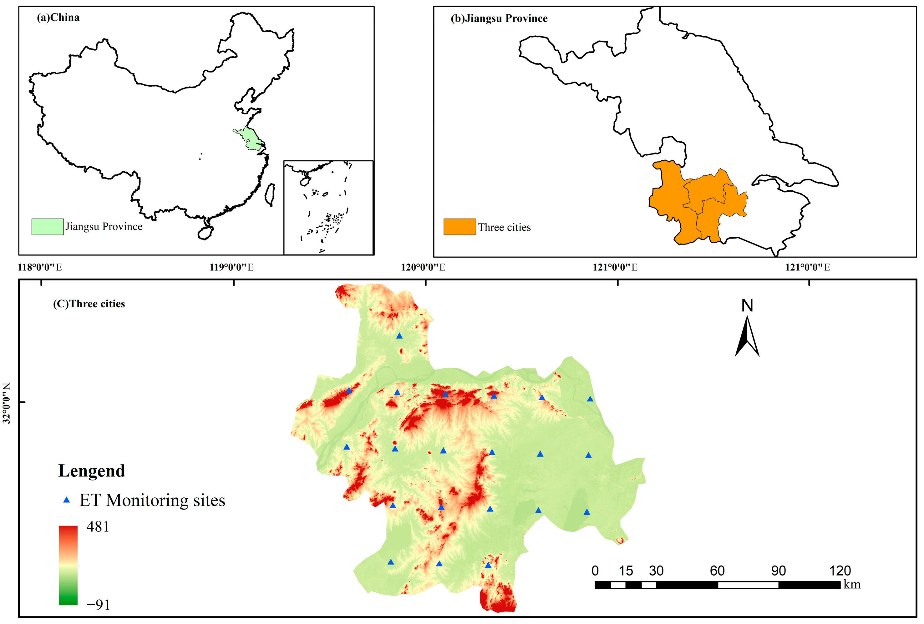
2.1. Study Area

The three cities (N 31°9′–32°36′, E 118°21′–120°11′) are located in the southwest of Jiangsu Province, and the monitoring stations are laid out as shown in Figure 1. With a total area of 14,785 km2 and a population of 16,677,400, the three cities have a gently sloping terrain with an average altitude of 50 m above sea level and are located in a subtropical monsoon climate zone with abundant rainfall of 1200 mm per year and an average annual temperature of 15.4 °C. Due to its location in the lower reaches of the Yangtze River and the Huai River, the total length of the coastline along the river is nearly 360 km, and a large alluvial plain makes up the rich arable land resources, with an arable land area of 406,000 hectares, and an annual grain production of over 35 million tons, making it one of the 13 major grain-producing areas in China.

2.2. Data Acquisition

2.2.1. Satellite Data

The remote sensing data selected for this study were the Landsat 8 OIL_TIRS data (https://www.gscloud.cn/, accessed on 17 February 2023), developed by NASA in collaboration with the United States Geological Survey (USGS). The satellite data are for the years 2016–2021 (the year 2020 is not included in this paper due to the poor results of the 2020 satellite data), and information about the data is shown in Table 1.
The remote sensing data were pre-processed with ENVI5.3 for image fusion (fusion of multispectral bands with panchromatic bands to improve image resolution), radiometric correction, and atmospheric correction. Based on the GPS coordinates of the monitoring points, the average reflectance of the samples in the monitoring area was extracted as the spectral reflectance of the sampling point by plotting the region of interest (ROI), and the spectral reflectance data of different wavelengths were obtained.

2.2.2. Meteorological Data

The meteorological information for the study area was obtained from the China Meteorological Data Network (https://data.cma.cn/, accessed on 17 February 2023). The monitoring station layout is consistent with the actual ET measurement points. Zhang et al. [30] pointed out that the soil temperature and surface temperature (LST) are closely related and their temporal variability tends to show similar characteristics. However, this similarity is largely dependent on the influence of meteorological factors and the physical properties of the subsurface (soil heat flux, vegetation cover, snow cover, etc.); therefore, LST data do not truly reflect the true soil temperature, and thus cannot produce more accurate predictions and simulations of soil ET. In summary, the meteorological variables recorded included the air temperature, relative humidity, net solar radiation, and soil temperature and humidity.

2.2.3. Measured ET Data

The actual ET data for this study were obtained from 21 ET monitoring stations in the study area (Figure 1), with the stations evenly distributed according to the latitude and longitude grid. The data collected in this study included the daily actual ET, monthly actual ET, and annual actual ET at each site in 2016–2021, where the time of collection was aligned with the time of the remote sensing images.

2.3. Vegetation Index Construction

Vegetation indices are spectral indices made up of different combinations of wavebands. They are a simple and effective empirical measurement method for different features and their characteristic information, and are widely used in remote sensing monitoring of soil parameters, crop growth, environmental changes, etc. [31,32,33,34]. In this study, 14 vegetation indices were selected as indicators for constructing the ET inversion model of the study area according to the requirements of the evapotranspiration inversion, as shown in Table 2.
Vegetation indices are linear or non-linear combinations of different bands in remote sensing data, which result in a high degree of linear correlation between vegetation counts. In multiple linear regression and multiple regression models, strong correlations between the independent variables can lead to unstable estimates, which can affect the accuracy of the model and its later replication [47]. The correlation between the independent variables can be measured using the variance inflation factor (VIF), which is generally considered to be strong when VIF > 10. The principle of VIF is as follows:
V I F j = 1 1 R j 2 , j = 1 , , p
where Rj represents the negative correlation coefficient of the independent variable on the remaining independent variables for regression analysis, and p is the number of all independent variables.

2.4. Data Dimensionality Reduction

2.4.1. Cluster Analysis

In the actual modeling process, as most of the vegetation indices reflect the vegetation physiology, soil water content, etc., some of the vegetation indices have the same or a similar meaning for ET interpretation, which may lead to a more redundant model. Therefore, under the condition that the information contained in the vegetation indices is not affected, some of the spectral indices can be clustered and analyzed, and a reasonable number of classifications can be selected for data dimensionality reduction according to the results of the clustering analysis.

2.4.2. Factor Analysis

Factor analysis (FN) is a generalization and development of principal component analysis. FN combines objects (variables or samples) with complex relationships into a small number of factors, retaining the intrinsic links between the factors and the original variables while diluting the linear relationships between the factor variables. The formula for the principle of factor analysis is as follows:
X 1 = a 11 F 1 + a 12 F 2 + + a 1 m F m + ε 1
X 2 = a 21 F 1 + a 22 F 2 + + a 2 m F m + ε 2
X p = a p 1 F 1 + a p 2 F 2 + + a p m F m + ε p
where aij represents the factor loading; A = (aij) is the factor loading matrix; ε is the special factor.
The factor score function is derived from the factor analysis model as follows:
F j = a j 1 X 1 + a j 2 X 2 + + a j p X p j = 1 , 2 , , m

2.5. Determination of Important Parameters

2.5.1. Ecosystem Parameters

ET is the total flux of water vapor transported to the atmosphere by vegetation and the ground and consists mainly of vegetation transpiration and soil water evaporation. The intensity of soil water evaporation is mainly influenced by the soil water content, soil temperature, and soil structure. In 1998, the Food and Agriculture Organization of the United Nations (FAO) proposed Penman–Monteith as the only standard for calculating the evaporation of vegetation (ET0). ET0 is calculated as follows:
ET 0 = 0.408 Δ ( R n G ) + r 900 T + 273 u 2 ( e s e a ) Δ + r ( 1 + 0.34 u 2 )
where ET0 is the reference evapotranspiration, mm/day; Rn is the net radiation on the crop surface, MJ/(m2⋅day); G is the soil heat flux, MJ/(m2⋅day); T is the average daily temperature at an altitude of 2 m, °C; u2 is the wind speed at a height of 2 m, m/s; es is the saturated water vapor pressure, kPa; ea is the actual water vapor pressure, kPa; esea is the saturated vapor pressure difference, kPa; ∆ is the slope of the saturated water vapor pressure curve; r is the hygrometer constant, kPa/°C.
In summary, the variables of soil heat flux (Qs), soil temperature (Ts) and moisture (Th), and net solar radiation (D) were introduced as predictive variables to the input model, taking into account the influences of vegetation transpiration and soil evaporation.

2.5.2. Fractional Vegetation Cover

Fractional vegetation cover (FVC) is the percentage of vegetation (including leaves, stems, and branches) per unit area of the vertical projection of vegetation. FVC directly affects soil moisture retention capacity and regional plant water content, and thus surface evapotranspiration. In this study, FVC was calculated based on the two-dimensional pixel model (DPM) with the following equation:
F V C = N D V I N D V I s o i l N D V I v e g N D V I s o i l
where NDVIsoil is the NDVI value of bare land, and NDVIveg is the NDVI value of the area covered by vegetation.

2.6. Model and Accuracy Evaluation
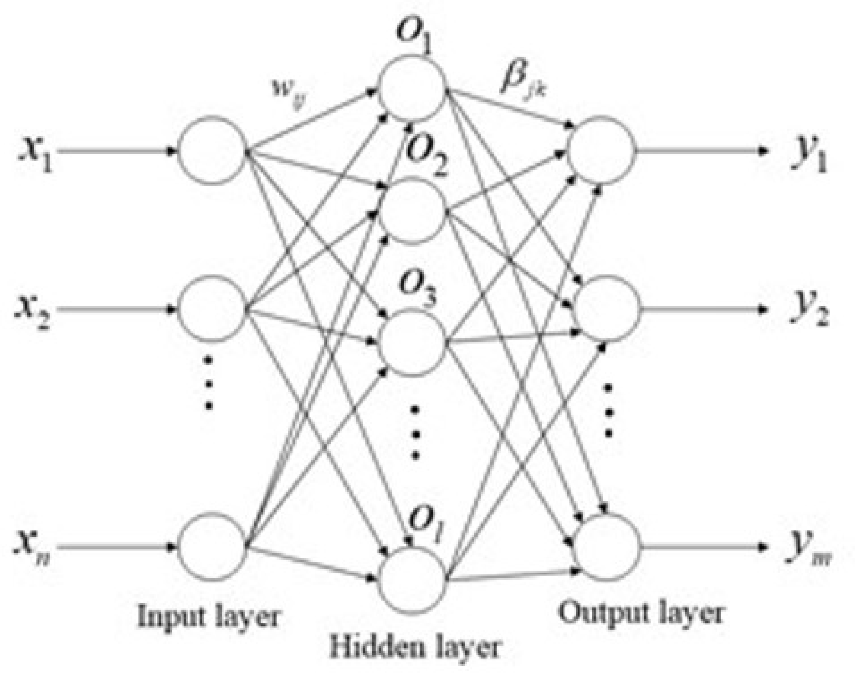
2.6.1. ELM

ELM is a new learning algorithm for single hidden layer feedforward neural networks (SLFNs) proposed by Huang et al. [48,49]. The essence of ELM is that the learning parameters of the hidden layer are randomly assigned and do not need to be adjusted, while the output weights can be determined via simple generalized inverse matrix operations [50]. Compared to other traditional SLFNs, ELM has a faster learning speed, better generalization performance, and minimal human intervention.
The principle of ELM is shown in Figure 2.
The above structure can be expressed by the formula
T = [ t 1 , t 2 , , t Q ] m × Q , t j = [ t 1 j t 2 j t m j ] = [ i = 1 l β i 1 g ( ω i x j + b i ) i = 1 l β i 2 g ( ω i x j + b i ) i = 1 l β i m g ( ω i x j + b i ) ] m × 1 ( j = 1 , 2 , , Q )
Equation (8) can be rewritten as
H β = T
where T is the full output; L is the number of hidden layers; g(x) are the activation functions; n is the number of input layers; w and β are the connection weights between the layers; H is the implied layer output matrix.

2.6.2. Multiple Linear Regression

Multiple linear regression analysis is a multivariate statistical technique used to examine the relationship between a single dependent variable and a set of independent variables [51]. MLR forecasting models are expressed in the following format:
Y t = X t β + ε t
where Yt is the predicted value at time t, Xt = (1, x1t, x2t, …, xkt) is a vector of k explanatory variables at time t, β = (β0, β1, …, βk) is the vector of coefficients, and εt is a random error term at time t. The errors terms should be independent and have a Gaussian distribution.

2.6.3. Accuracy Evaluation

In order to obtain the optimal model, the coefficient of determination (R2), root mean square error (RMSE), and rate of performance deviation (RPD) were used to evaluate the model and discuss the applicability of each model. R2 reflects the degree of fit between the predicted and measured values, and the closer its value is to 1, the better the model fits. The RMSE reflects the deviation between the predicted and measured values, and the smaller the value, the better the prediction effect of the model. The principles of each evaluation index are as follows:
R 2 = i = 1 n ( X i X ¯ ) 2 ( Y i Y ¯ ) 2 i = 1 n ( X i X ¯ ) 2 i = 1 n ( Y i Y ¯ ) 2
R M S E = i = 1 n ( Y i Y ¯ ) 2 n
R P D = i = 1 n V ¯ ( Y i ) 2 n R M S E

3. Results

3.1. Statistical Analysis of Measured ET

The measured ET data at each monitoring site from 2016 to 2021 were analyzed by year for descriptive statistics, and the sample data distribution is shown in Table 3. The data from each year were randomly partitioned using the trian_test_split dataset from the Python Scikit Learn library for the model training set and the test set, i.e., 90% of the samples were used for training and 10% were used for validation.

3.2. Variable Correlation Analysis

The correlation analysis of 21 spectral indices (7 band reflectance and 14 vegetation indices) and the measured ET in different years is shown in Table 4.

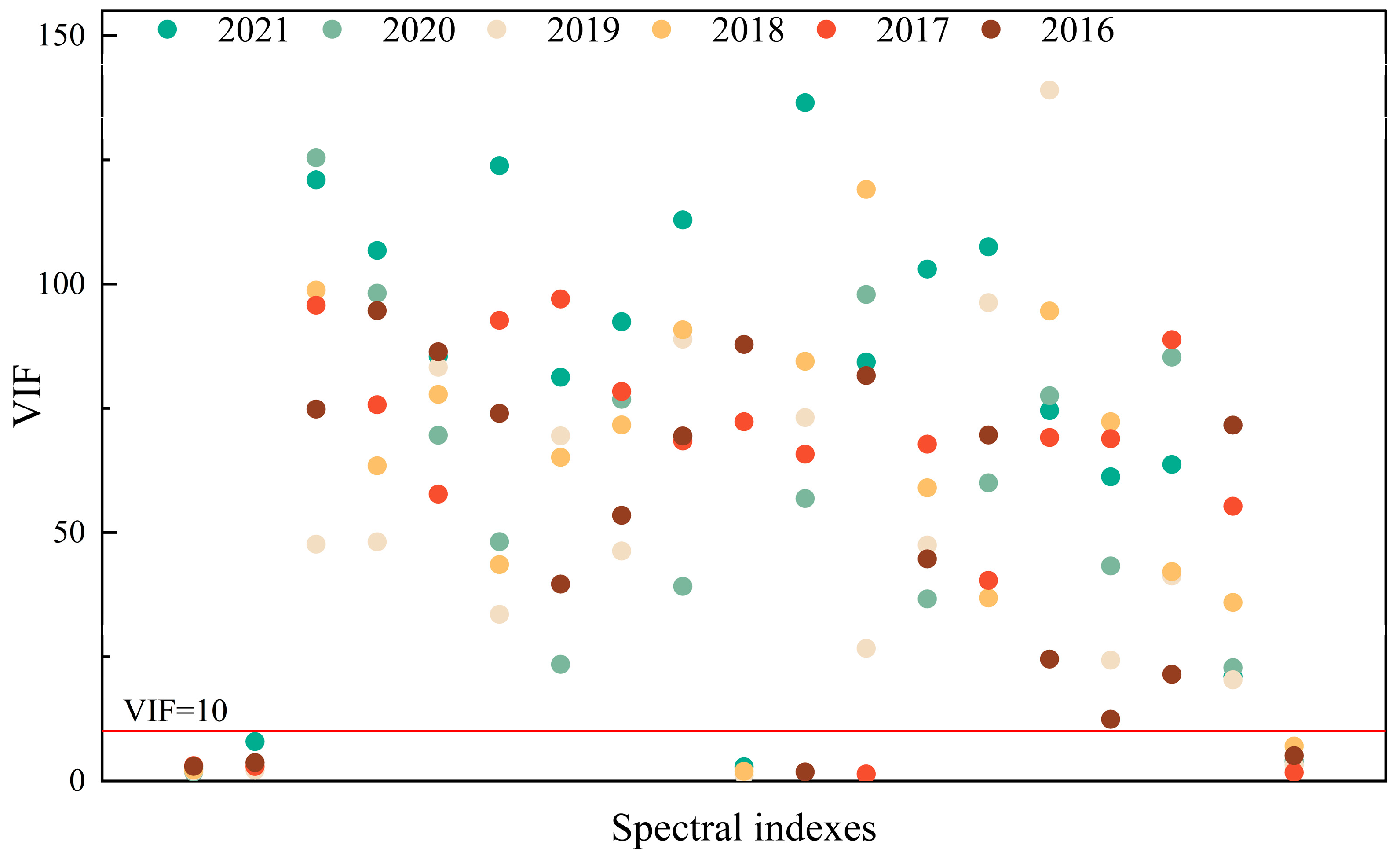
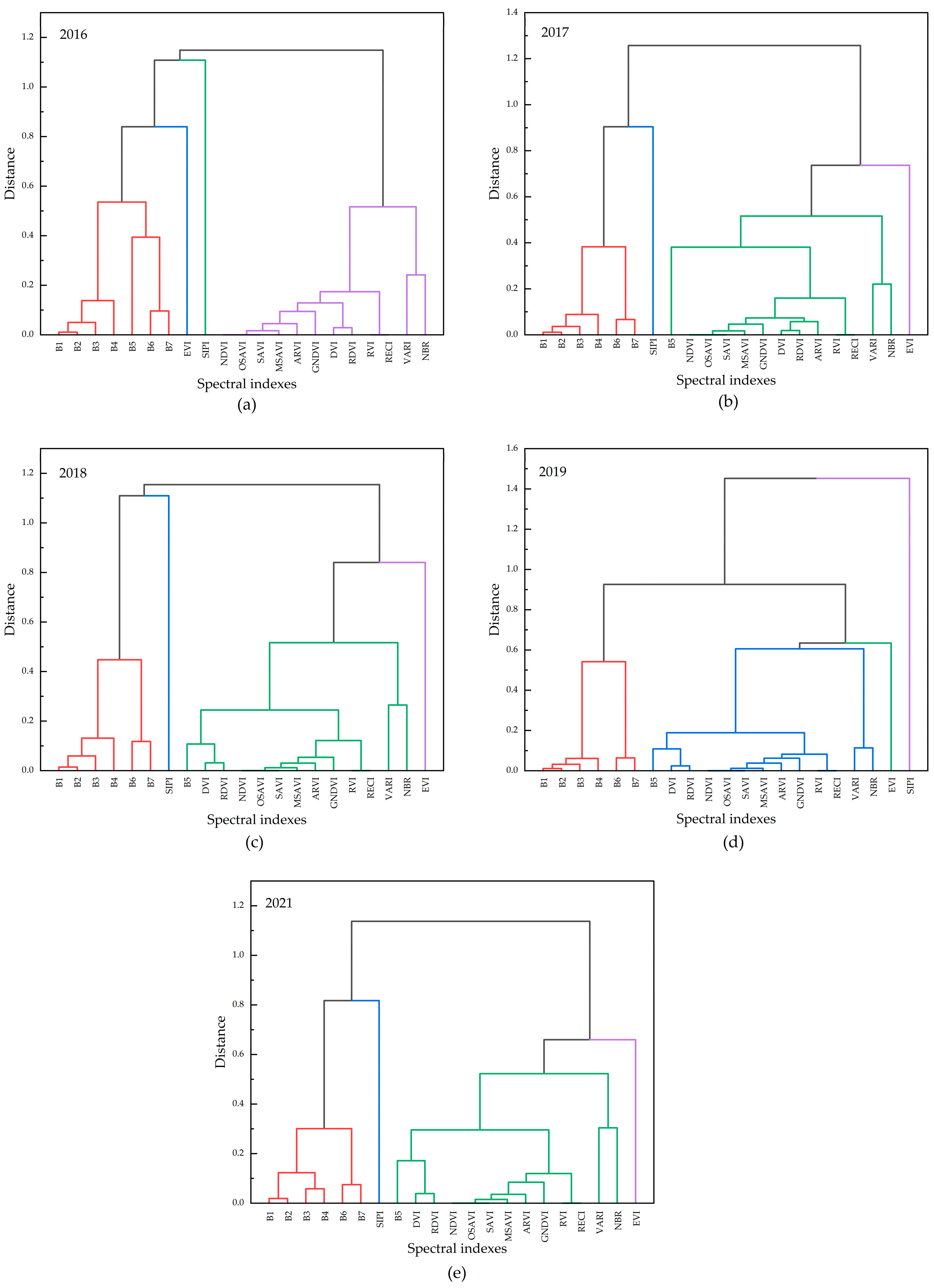
3.3. Data Dimensionality Reduction

The VIF between the spectral indices in this experiment is shown in Figure 3. The result showed that there was a serious problem of multicollinearity between the spectral indices.
According to Figure 3, it can be seen that there was strong multicollinearity between the spectral indices. In this paper, factor analysis and cluster analysis were used to extract potential collinearity factors to solve the collinearity problem.
Firstly, the spectrum indicators with severe covariance were clustered, and the output of the hierarchical cluster analysis pulse diagram after using the origin is shown in Figure 4.
As can be seen in Figure 4, the spectral indicators were divided into four categories for different years, with band reflectance B1 to B7 grouped together in different years as the different bands are still essentially electromagnetic spectra with similar interpretations of ground information.
Factor analysis was performed on the classes with a sample size greater than 1 in the clustering results. With a KMO of 0.6 to 0.8 and a p-value of 0.000 *** for the significance of Bartlett’s spherical test, the factor analysis was valid. The original spectral indices of the different classes were substituted into the factor analysis score function, and the results obtained were recombined with the spectral indices of the individual classes to form new spectral indices, denoted as F1, F2, F3, and F4. The results of the collinearity test of the new spectral indices are shown in Table 5.
By comparing the data and analysis in Figure 4 and Table 4, it can be seen that the VIF of the independent variables was reduced to below 10 after the dimensionality reduction of the cluster factor analysis, and the collinearity between the variables was basically resolved, which improved the stability of the model.

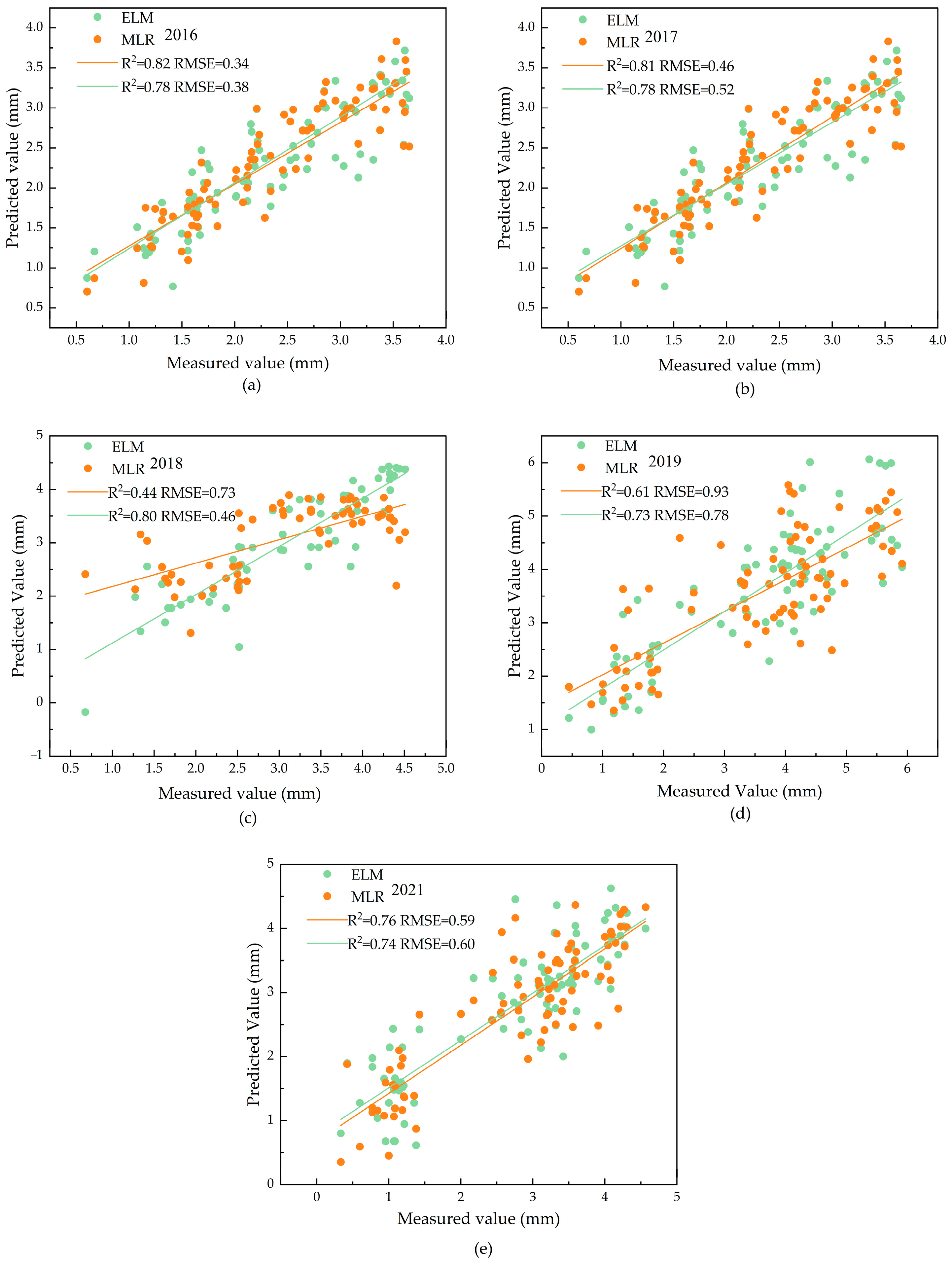
3.4. Results of Model Inversions

The four new spectral indices and four characteristic factors affecting ET changes through factor analysis were selected as independent variables, and the measured ET values of 21 meteorological stations in the three cities in 2016, 2017, 2018, 2019, and 2021 were used as dependent variables to construct an ET inversion model based on the ELM and MLR models. The results of the model construction are shown in Table 6. Only spectral parameters were selected to construct the model results, as shown in Table 7.
From Table 6, it can be concluded that the top three ranked models in terms of accuracy were 2021-MLR, 2017-ELM, and 2017-MLR, with an Rv2 of 0.87, 0.86, and 0.85, respectively, after combining the three evaluation indicators (R2, RMSE, and RPD); the lowest accuracy was found for 2019-MLR, with an Rv2 of 0.59, which showed a more obvious decrease compared with the models of the other years, because the cloud coverage of the Landsat satellite images was larger in 2019 and there were errors in the surface reflectance extracted via remote sensing.
Comparing the results in Table 6 with those in Table 7, it was found that when only spectral parameters were introduced as independent variables, the highest Rv2 was found for 2016-ELM and 2018-MLR, which was only 0.57, much lower than the model accuracy when ET feature parameters were fused under the same model; the reason for this is that, when only spectral parameters were used as independent variables for inversion, the mechanism of interaction between ET and each spectral parameter was unclear, and it was more difficult to perform the inversion through mathematical models. The characteristic parameters, as triggers of ET, are themselves highly correlated with ET, and their introduction as independent variables can effectively explain the correlation between the dependent and independent variables [20].
In order to verify the accuracy of the two models in different years, the predicted–measured scatter plots of the ELM and MLR validation sets were plotted using the measured ET values of the three cities from 2016 to 2021, as shown in Figure 5. There was a good linear relationship between the estimated and measured values of the two models (R2 > 0.44, RMSE < 0.08 mm), and the sample points on both sides of the regression line were evenly distributed. The MLR model had the best estimation in 2016, 2017, and 2021, with an R2 ranging from 0.76 to 0.82, but the estimation in 2018 was relatively poor, with an R2 of 0.44. Meanwhile, the ELM model had higher accuracy (R2 > 0.73, RMSE < 0.02 mm) in different years, with a more concentrated sample distribution.

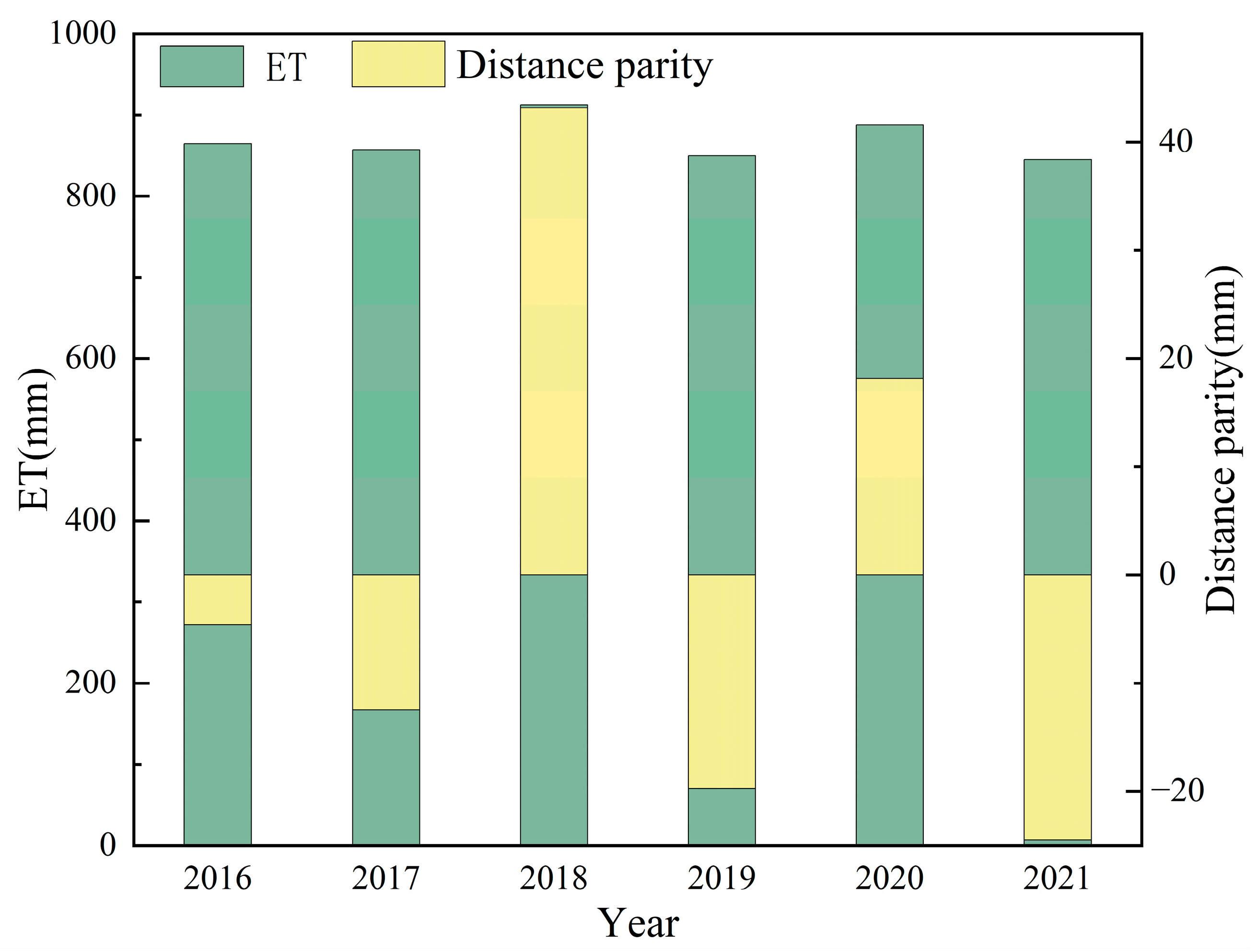
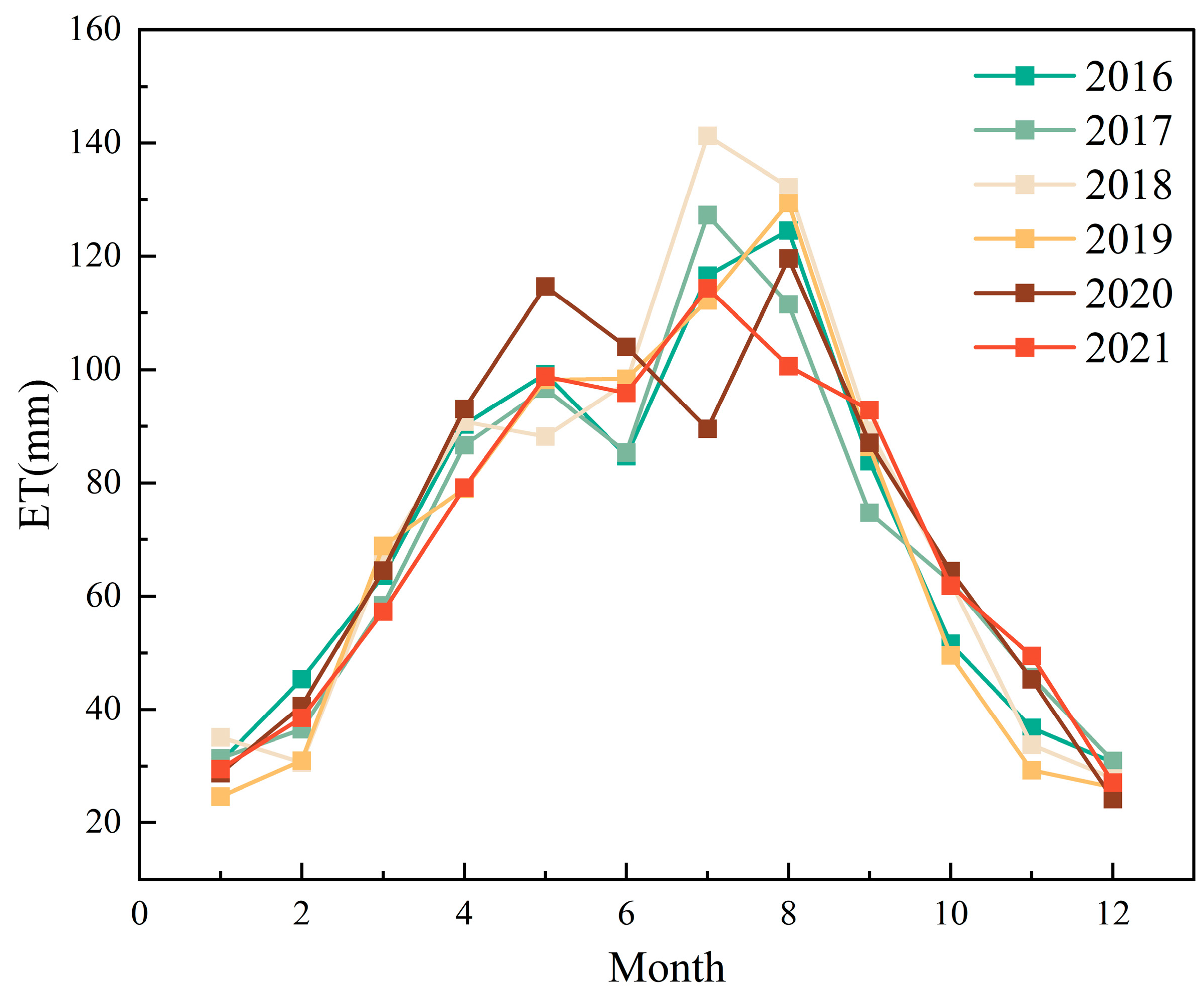
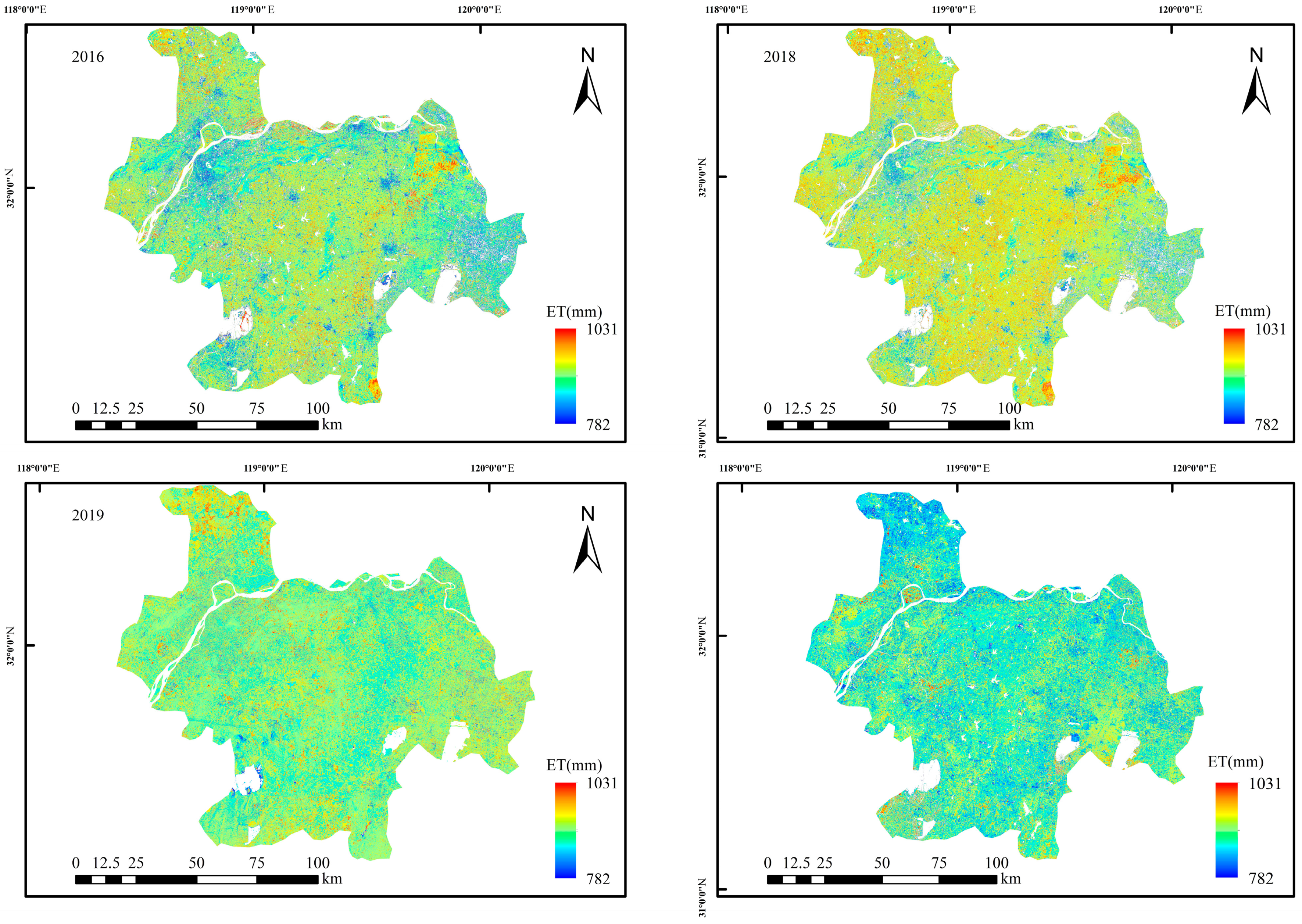
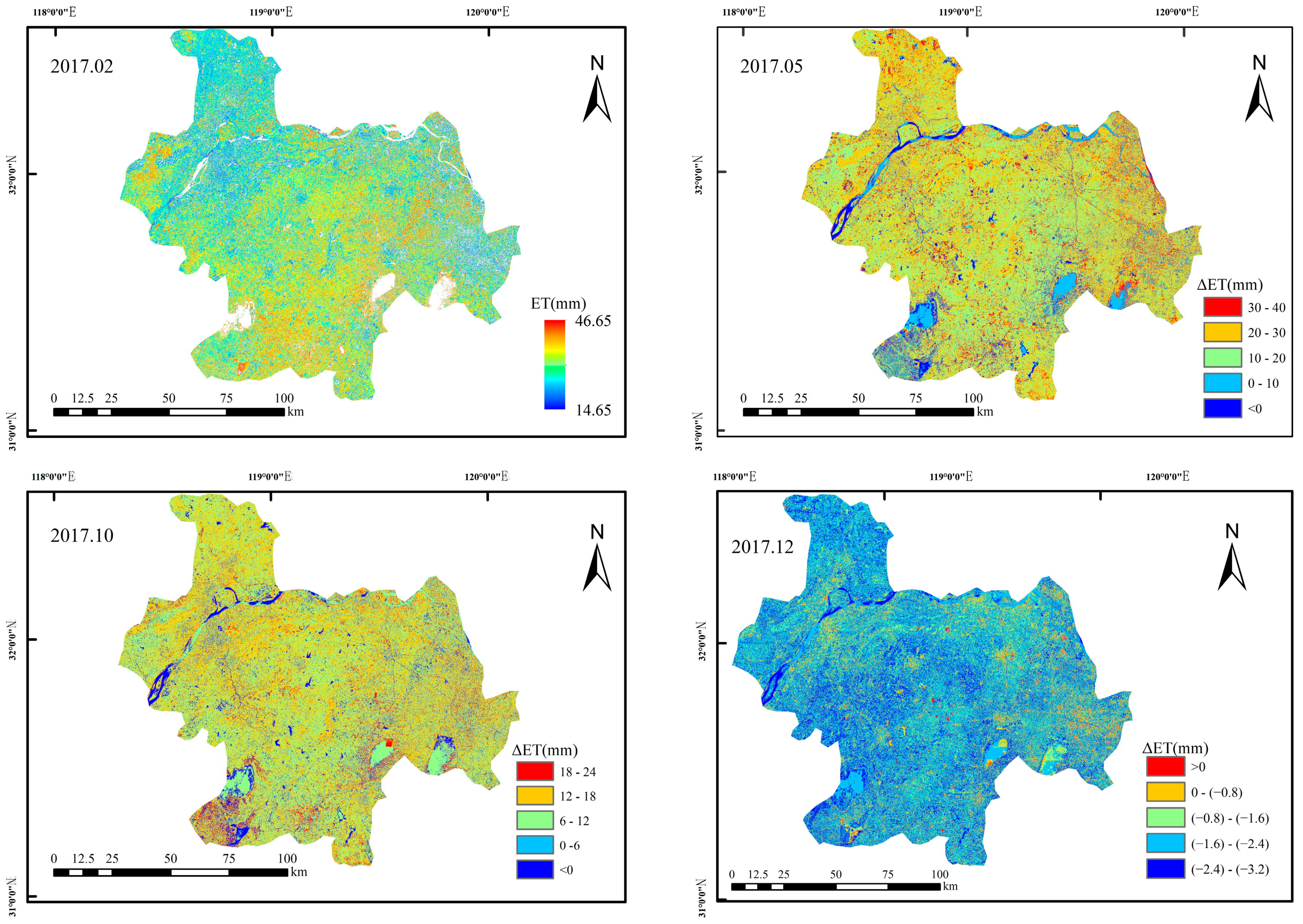
3.5. Analysis of the Distribution Characteristics of Evapotranspiration in the Three Cities

3.5.1. Time-Series Change Characteristics

As shown in Figure 6, the multi-year average of evapotranspiration in the three cities from 2016 to 2021 was 869.51 mm, with the maximum value of 912 mm occurring in 2018 and the minimum value of 845 mm occurring in 2021. Except for the years 2018 and 2020, the distance level of evapotranspiration in all the other years was negative and decreased year by year.
The variation in evapotranspiration by month in the study area from 2016 to 2021 is shown in Figure 7. Evapotranspiration rose continuously from January, fluctuated slightly in May, continued to rise to a peak in July–August, and then began to decline, with the minimum value during the year usually occurring in December, with evapotranspiration mainly concentrated in April–August during the year.

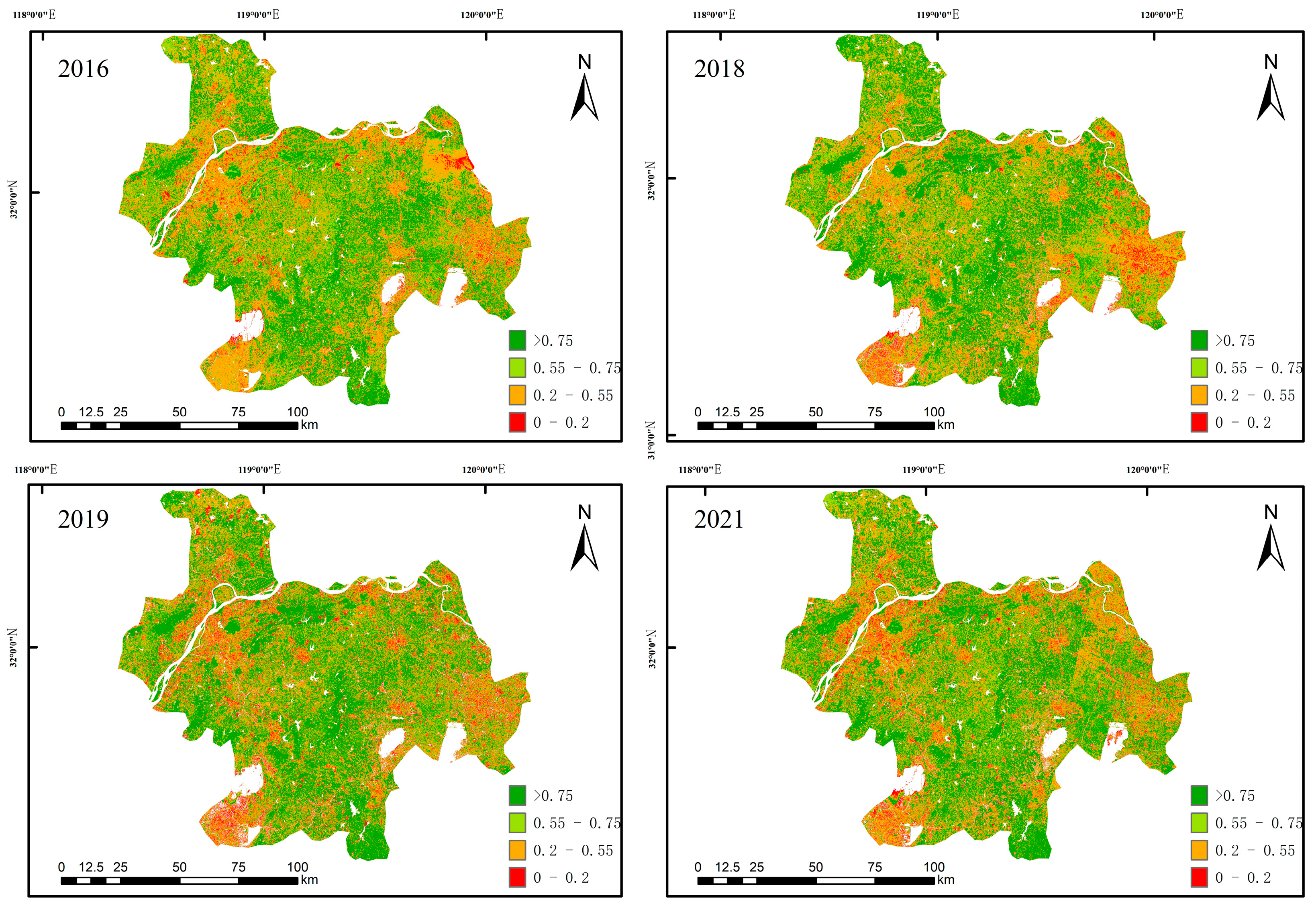
3.5.2. Inter-Annual Spatial Distribution Characteristics

Based on the ET remote sensing estimation model constructed in Section 3.4, the year-by-year data of the study sites were imported into the model. The inversion of the spatial distribution of inter-annual changes from 2016 to 2021 is shown in Figure 8. As can be seen in Figure 8, the areas with higher ET were mainly concentrated in the rural areas north of the Yangtze River and the central and western plains where agricultural land is concentrated, while the urban areas in the study area had lower evapotranspiration due to having less bare soil and cultivated land area and a lower vegetation cover. During the study years, ET ranged from 782 to 979 mm in 2016; in 2018, evapotranspiration increased significantly, with 87% of the study area having inter-annual ET greater than the multi-year average evapotranspiration; in 2019, ET in the study area began to decline slowly, with 51.82% of the total study area having inter-annual ET above the multi-year average evapotranspiration; in 2021, ET decreased significantly, with an average inter-annual evapotranspiration of only 845 mm. This is a decrease of 24 mm compared to the multi-year average evapotranspiration.

3.5.3. Seasonal Spatial Distribution Characteristics

Taking 2017 as an example, the intra-annual variation and distribution characteristics of ET based on month-by-month data are shown in Figure 9. The spatial distribution of evapotranspiration in all four seasons was basically consistent with the spatial distribution throughout the year, with high-value areas distributed in areas with high vegetation cover and obvious farmland features, especially in the north and central-west, and lower evapotranspiration along the Yangtze River and near urban clusters. ET changes in the study area all showed obvious seasonal characteristics, with evapotranspiration in February ranging from 14.65 to 46.65 mm, with an average evapotranspiration of 36 mm, and high-evapotranspiration areas mainly concentrated in forests and spring-wheat-growing areas in the central and western parts of the study area. Evapotranspiration in May (summer) was significantly higher, and compared to February, evapotranspiration throughout the study area was increased by more than 10 mm, except for some water bodies that were not included in the study. The evapotranspiration was slightly greater in October (autumn) than in February, with an overall change of 6–18 mm, accounting for 84.83% of the total study area. December (winter) had the least evapotranspiration, with a significant decrease compared to spring, with 90.65% of the study area reduced by 1.6–3.2 mm.

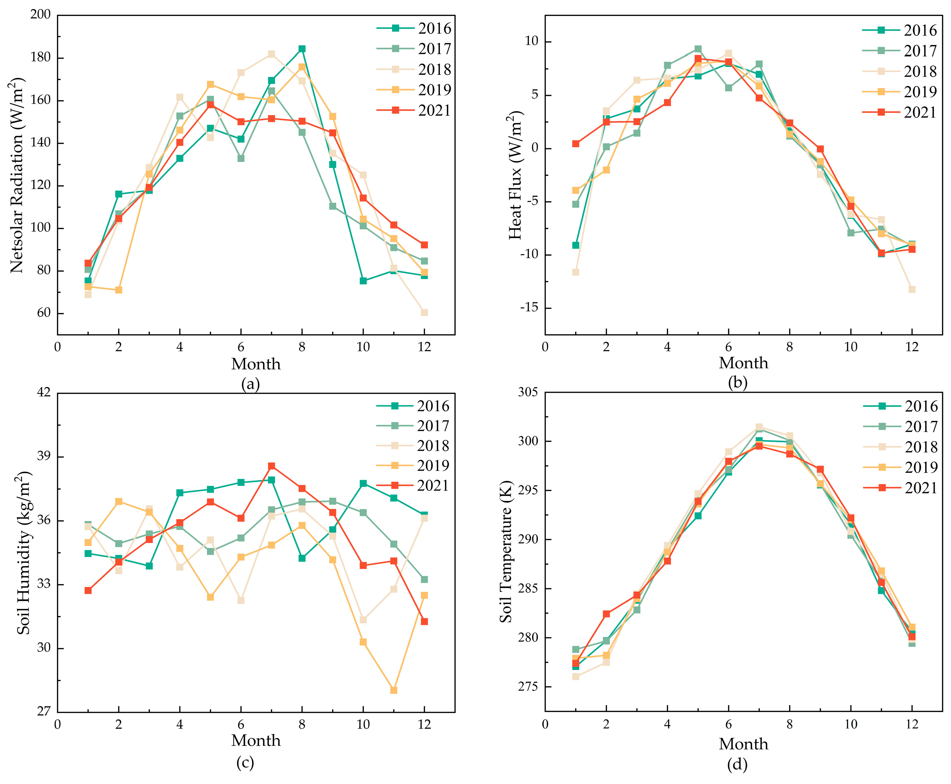
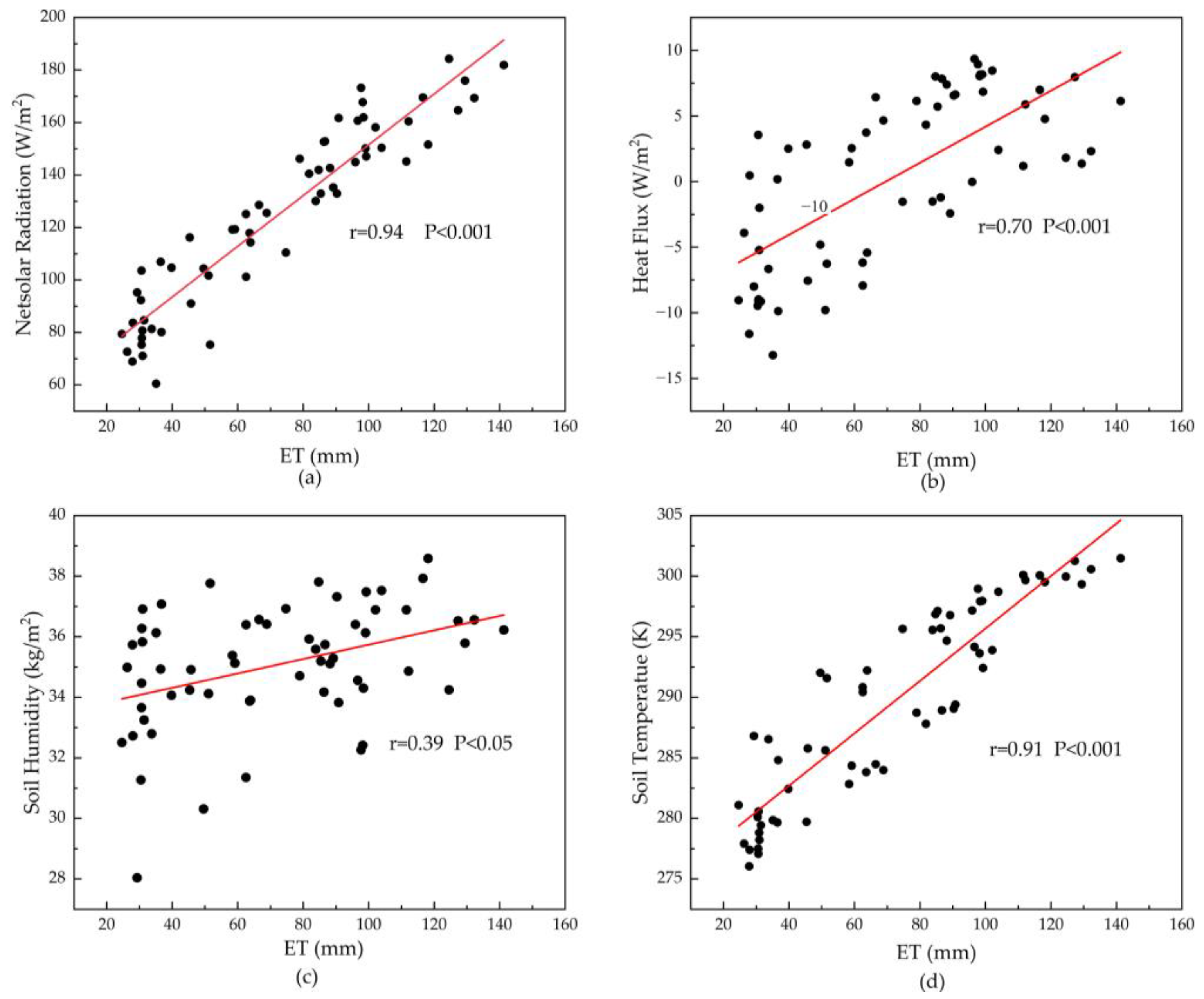
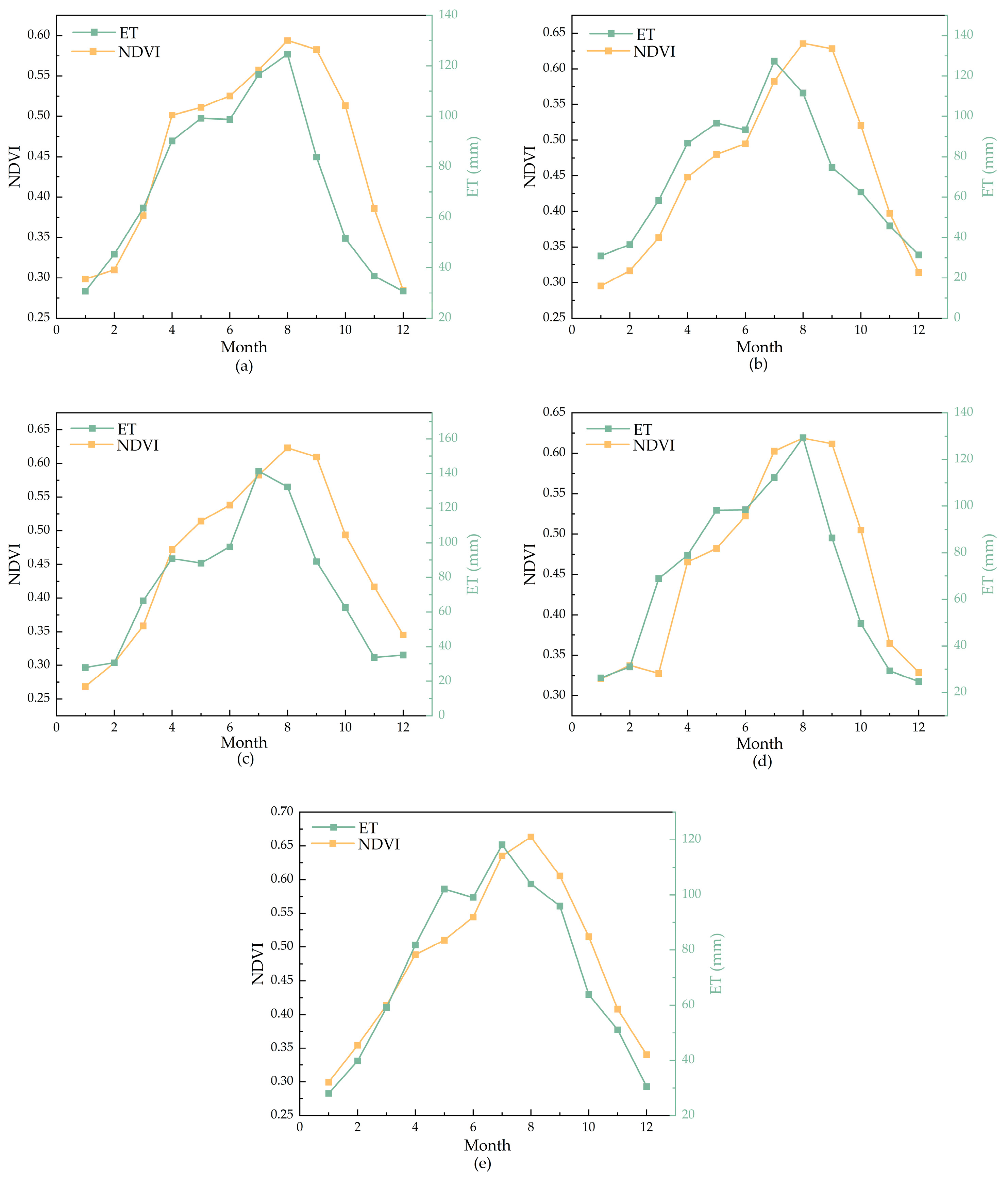
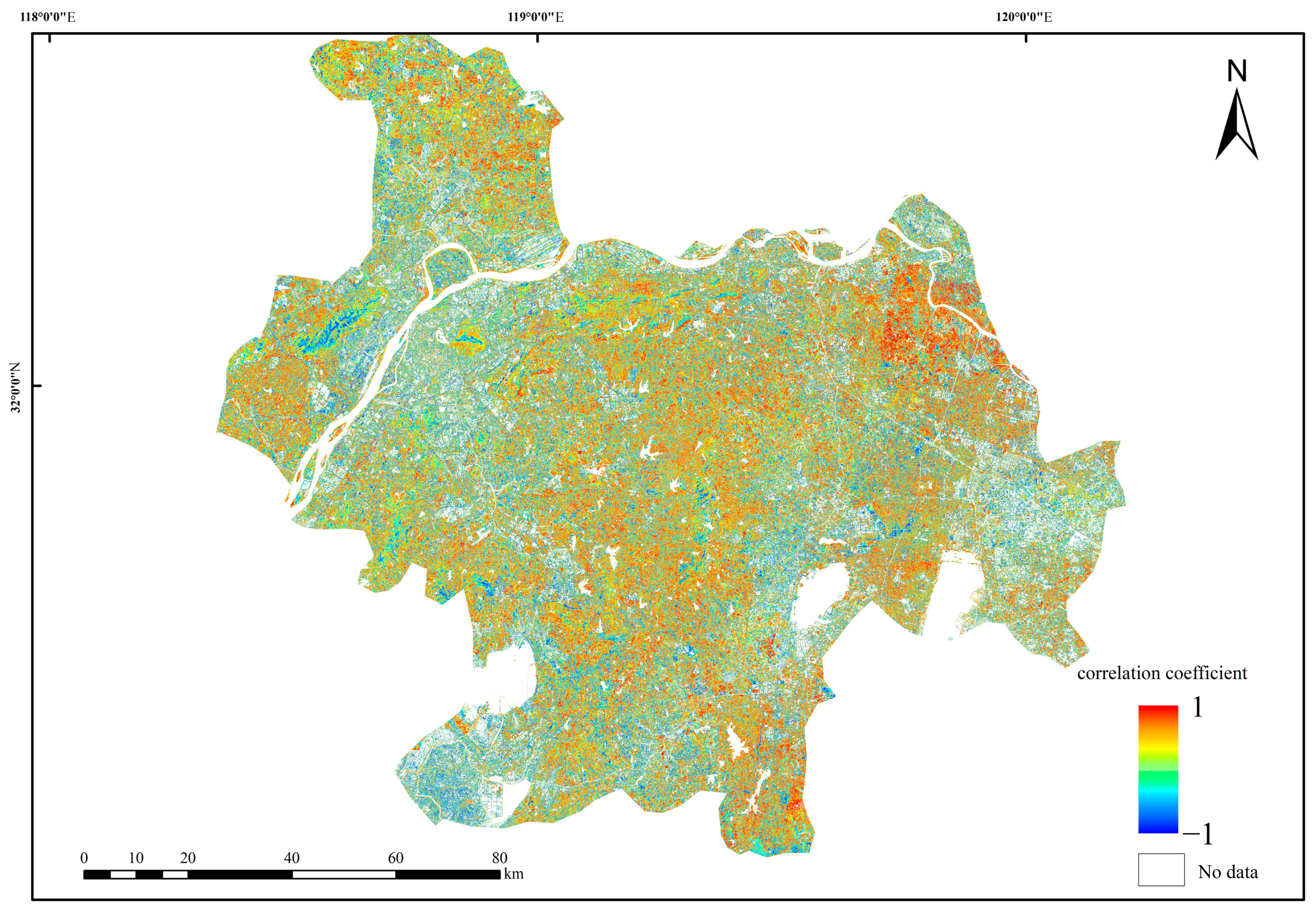
3.6. Analysis of Characteristic Factor Drivers

3.6.1. Environmental Factors

As the most direct receptors of climate change, ecological and environmental factors play an irreplaceable role in all aspects of the ecosystem. To explore the influence of meteorological factors on regional ET, the characteristics of the changes in the mean solar net radiation intensity, soil heat flux, and soil temperature and humidity in the study area from 2016 to 2021 were statistically analyzed, as shown in Figure 10. From Figure 10, it can be seen that, except for the fluctuation in soil moisture, the net solar radiation intensity, soil heat flux, and soil temperature and humidity all showed strong seasonal characteristics, with an increasing trend from January to June and a decreasing trend from August to December, with peaks occurring in July and August, which were basically consistent with the changes in ET during the year. To explore the correlation between the above four environmental factors and the dynamic changes in ET in the study area, the correlation between ET and each of the four environmental factors was calculated for each month from 2016 to 2021, as shown in Figure 11. From Figure 11, it can be seen that the net solar radiation, soil temperature, and soil heat flux had highly significant effects on ET in the study area, with correlation coefficients of 0.94, 0.91, and 0.70 (p < 0.01), respectively. In addition, soil moisture also had a significant effect on ET in the study area, with a correlation coefficient of 0.39 (p < 0.05).

3.6.2. Factors of FVC

FVC directly affects the soil water holding capacity and the water content within regional plants, thus affecting the amount of surface evapotranspiration [52]. The FVC and ET change curves for the study area from 2016 to 2021 are shown in Figure 12. As can be seen in the figure, FVC had a positive effect on surface evapotranspiration, and both curves are periodic single-peaked curves. From March to August, with the growth of plants, the water in plants increased and the density of FVC increased, providing moisture conditions for surface evapotranspiration. ET and FVC showed a significant upward trend and reached a peak in August–September, and from September to December, due to weather changes, plants started to wilt, and thus FVC and ET declined from September to December, which continued until February of the following year.
The distribution of FVC in the three cities from 2016 to 2021 is shown in Figure 13. Its spatial distribution was basically consistent with the spatial distribution of ET in the same period. The northern, central, and southwestern areas of the study area are mostly cultivated land and natural forest land, where the spatial distribution of vegetation is dense and the soil water content is high, meaning the transpiration of plants and soil evaporation are higher than those in other areas. The spatial distribution of the correlation coefficients between ET and FVC is shown in Figure 14. This is mainly due to the fact that most of the positive-correlation areas are cultivated and forested, and bare soil and vegetation variations have a greater influence on ET.

4. Discussion

In this paper, using Landsat 8 remote sensing satellite images of the lower Yangtze River urban agglomeration from 2016 to 2021, we introduced five ecological and environmental factors involved in the Penman–Monteith equation: soil heat flux, soil temperature and humidity, net solar radiation, and vegetation cover, and established a multi-temporal ET prediction model based on ELM and MLR, with refined inversions of both models. The results were good, with an R2 above 0.59. In addition, the spatial and temporal variation characteristics of ET in the study area were analyzed through remote sensing visualization, and the driving forces of soil heat flux and other factors were analyzed and compared. The correlation coefficients showed that the net solar radiation, soil heat flux, soil temperature, and vegetation cover all significantly influenced the ET variation and greatly enhanced the accuracy of the prediction models. This finding indicates that the combination of spectral data and ecological data can be used to carry out the prediction and accuracy optimization of regional remote sensing ET.

4.1. Data Optimization Studies

For predictive models, correlations between predictors can have unpredictable and inconsistent effects on parameter estimates and significance, and may lead to biased results [53]. In most remote sensing inversion studies, researchers tend to ignore this issue or simply eliminate variables with strong covariance, which may result in the elimination of variables that contribute more to the model prediction at the expense of the accuracy of the model prediction. In this study, clustering analysis was used to group variables with the same information and perform factor analysis, which can effectively deal with the problem of multiple cointegration between variables and improve the model prediction accuracy and stability. The results showed that the VIF of the variables treated using the cluster factor analysis dropped to below 3, and the models could still maintain a high R2.

4.2. Model Accuracy Discussion

Many studies have shown that the use of machine learning models can show better predictive power in estimating ET [20]. Compared to the traditional PM equation, the introduction of spectral data, meteorological, and ecological data in this study yielded better predictors (R2 = 0.59−0.87, RMSE < 0.59) [54]. In addition, when comparing the machine learning model with the linear regression model in this study horizontally, the difference in inversion accuracy between the two was not significant, and even in some year types, the MLR prediction accuracy was higher than that of the ELM model. This is because machine learning techniques rely on a large amount of data to achieve high performance, and when the data samples are the same and have not reached their peak, the machine learning prediction effect does not prevail. In contrast, the traditional linear regression achieved good prediction results based on the theoretical causality of the data [55], while some of the induced factors introduced based on the PM equation, which itself has a good linear relationship with ET, greatly increased the explanatory power of the multiple linear regression for ET.

4.3. Selection of Vegetation Indices

NDVI, a widely used vegetation index, plays an important role in monitoring vegetation. However, environmental factors such as atmospheric conditions, topographical effects, and topographic illumination may affect it significantly [56]. Glenn et al. [57] found that the enhanced vegetation index (EVI), compared to NDVI, improved vegetation monitoring through a de-coupling of the canopy background signal and a reduction in atmospheric influences. However, the presence of soil regulators in EVI does not eliminate the influence of topographic effects and has limitations for estimating vegetation cover changes on a large scale. In addition, Moreira et al. [58] found that topographic illumination was negligible in areas where the average watershed slope was below 25° and the latitude was below 45°. From a review of the data, the study area (lower Yangtze River plain) has a relatively flat topography, with an average elevation of 20–30 m and an average slope of 2–6°; therefore, the choice of NDVI as a parameter for vegetation cover estimation has some applicability.

4.4. Spatial- and Temporal-Change-Driven Analysis

Spatially, the distribution of ET in the study area was basically in line with the general trend, mainly concentrated in areas with high vegetation cover such as farmland and forests in the urban periphery and extensive agricultural land. From a temporal perspective, ET showed more obvious seasonal variations within the year, mainly in summer > autumn > spring > winter. According to the analysis of the previous driving factors, ET changes are influenced by the net solar radiation intensity, soil heat flux, and soil temperature and humidity, and these four driving factors themselves are more sensitive to the season, thus leading to seasonal differences in ET. According to the mean ET values measured at each meteorological station, the maximum ET during the year was 912.67 mm in 2018, and the minimum was 845.02 mm in 2021, which is consistent with the results of this paper.

5. Conclusions

This paper took the lower Yangtze River urban agglomeration as the research object, combined Landsat 8 OIL_TIRS remote sensing data and five types of ecological environment data derived from the Penman–Monteith formula, constructed ET inversion models under different years and seasons based on the ELM and MLR models, and analyzed the distribution characteristics and influence factors of ET. The following conclusions were drawn:
  • It is feasible to build an ET inversion model using satellite remote sensing spectral data and ecological environment data. Both models could invert the ET in the study area with high accuracy, and the introduction of ecological environment factors significantly improved the model accuracy. Among them, the best model for inversion from 2016 to 2019 was the ELM model, with an R2 of 0.82, 0.86, 0.83, and 0.62, and an RMSE of 0.31 mm, 0.06 mm, 0.59 mm, and 0.29 mm, respectively; the best model for inversion in 2021 was the MLR model, with an R2 of 0.87 and an RMSE of 0.29 mm.
  • The spatial and temporal distributions of ET in the study area showed typical geographical and seasonal characteristics. Spatially, higher-ET areas were concentrated in the north, central, and south-western areas with higher vegetation cover and more extensive agricultural land; ET values were lower in areas close to cities. Temporally, ET peaked in summer, and the values of ET in all seasons, from high to low, followed the order summer > autumn > spring > winter.
  • Net solar radiation, soil heat flux, soil moisture, and soil temperature significantly affected the ET variation, with correlation coefficients of 0.94 (p < 0.001), 0.70 (p < 0.001), 0.39 (p < 0.05), and 0.91 (p < 0.001), respectively; the average correlation coefficient of vegetation cover reached 0.605, and its spatial and temporal variations were also the main factors in the increase or decrease in ET in the study area.

Author Contributions

Conceptualization, E.S. and X.Z.; methodology, G.S.; software, A.J.; validation, J.L., Y.Z. and L.T.; formal analysis, E.S.; investigation, G.S.; resources, E.S.; data curation, Y.Z.; writing—original draft preparation, E.S.; writing—review and editing, J.L.; visualization, A.J.; supervision, X.Z.; project administration, E.S.; funding acquisition, G.S. All authors have read and agreed to the published version of the manuscript.

Funding

This research was funded by the National Natural Science Foundation of China, grant number 51879072, and the Jiangsu Water Conservancy Science and Technology Project, grant number 2015087.

Data Availability Statement

The data presented in this study are available on request from the corresponding author.

Acknowledgments

We would like to acknowledge the remote sensing data provided by NASA and the actual measured ET data provided by the meteorological monitoring sites in Nanjing. The authors extend their gratitude to the editor and anonymous reviewers for substantial comments on earlier version of this paper.

Conflicts of Interest

The authors declare no conflict of interest.

References

  1. Wang, J.; Cheng, D.; Wu, L.; Yu, X. Remote-Sensing Inversion Method for Evapotranspiration by Fusing Knowledge and Multisource Data. Sci. Program. 2022, 2022, 2076633. [Google Scholar] [CrossRef]
  2. Zhang, K.; Kimball, J.S.; Running, S.W. A review of remote sensing based actual evapotranspiration estimation. Wiley Interdiscip. Rev.-Water 2016, 3, 834–853. [Google Scholar] [CrossRef]
  3. Anderson, M.C.; Zolin, C.A.; Sentelhas, P.C.; Hain, C.R.; Semmens, K.; Yilmaz, M.T.; Gao, F.; Otkin, J.A.; Tetrault, R. The Evaporative Stress Index as an indicator of agricultural drought in Brazil: An assessment based on crop yield impacts. Remote Sens. Environ. 2016, 174, 82–99. [Google Scholar] [CrossRef]
  4. Khan, A.; Stockle, C.O.; Nelson, R.L.; Peters, T.; Adam, J.C.; Lamb, B.; Chi, J.; Waldo, S. Estimating Biomass and Yield Using METRIC Evapotranspiration and Simple Growth Algorithms. Agron. J. 2019, 111, 536–544. [Google Scholar] [CrossRef]
  5. Yang, Y.; Anderson, M.C.; Gao, F.; Wardlow, B.; Hain, C.R.; Otkin, J.A.; Alfieri, J.; Yang, Y.; Sun, L.; Dulaney, W. Field-scale mapping of evaporative stress indicators of crop yield: An application over Mead, NE, USA. Remote Sens. Environ. 2018, 210, 387–402. [Google Scholar] [CrossRef]
  6. Oliveira, R.A.; Rocha, I.d.B.; Sediyama, G.C.; Puiatti, M.; Cecon, P.R.; Silveira, S.d.F.R. Coeficientes de cultura da cenoura nas condições edafoclimáticas do Alto Paranaíba, no Estado de Minas Gerais. Rev. Bras. De Eng. Agrícola E Ambient. 2003, 7, 280–284. [Google Scholar] [CrossRef]
  7. Faisol, A.; Indarto; Novita, E.; Budiyono. An evaluation of MODIS global evapotranspiration product (MOD16A2) as terrestrial evapotranspiration in East Java—Indonesia. In Proceedings of the 2nd International Conference on Environmental Geography and Geography Education (ICEGE), Univ Jember, FKIP, Dept Social Sci Educ, East Java, Indonesia, 28–29 September 2020. [Google Scholar]
  8. Eugenio, F.; Marcello, J.; Martin, J. High-Resolution Maps of Bathymetry and Benthic Habitats in Shallow-Water Environments Using Multispectral Remote Sensing Imagery. IEEE Trans. Geosci. Remote Sens. 2015, 53, 3539–3549. [Google Scholar] [CrossRef]
  9. Yao, L.; Lu, N. Spatiotemporal distribution and short-term trends of particulate matter concentration over China, 2006–2010. Environ. Sci. Pollut. Res. 2014, 21, 9665–9675. [Google Scholar] [CrossRef]
  10. Li, H.; He, X.; Ding, J.; Bai, Y.; Wang, D.; Gong, F.; Li, T. The Inversion of HY-1C-COCTS Ocean Color Remote Sensing Products from High-Latitude Seas. Remote Sens. 2022, 14, 5722. [Google Scholar] [CrossRef]
  11. Lopez, O.; McCabe, M.F.; Houborg, R. Evaluation of multiple satellite evaporation products in two dryland regions using GRACE. In Proceedings of the 21st International Congress on Modelling and Simulation (MODSIM) held jointly with the 23rd National Conference of the Australian-Society-for-Operations-Research/DSTO led Defence Operations Research Symposium DORS, Gold Coast, Australia, 29 November–4 December 2015; pp. 1379–1385. [Google Scholar]
  12. McCabe, M.F.; Miralles, D.G.; Holmes, T.R.H.; Fisher, J.B. Advances in the Remote Sensing of Terrestrial Evaporation. Remote Sens. 2019, 11, 1138. [Google Scholar] [CrossRef]
  13. Chen, J.M.; Liu, J. Evolution of evapotranspiration models using thermal and shortwave remote sensing data. Remote Sens. Environ. 2020, 237, 111594. [Google Scholar] [CrossRef]
  14. Wang, S.; Liu, C.; Tan, Y.; Wang, J.; Du, F.; Han, Z.; Jiang, Z.; Wang, L. Remote sensing inversion characteristic and driving factor analysis of wetland evapotranspiration in the Sanmenxia Reservoir area, China. J. Water Clim. Change 2022, 13, 1599–1611. [Google Scholar] [CrossRef]
  15. Gao, H.; Zhang, X.; Wang, X.; Zeng, Y. Phenology-Based Remote Sensing Assessment of Crop Water Productivity. Water 2023, 15, 329. [Google Scholar] [CrossRef]
  16. Yang, Y.; Yang, Y.; Liu, D.L.; Nordblom, T.; Wu, B.; Yan, N. Regional Water Balance Based on Remotely Sensed Evapotranspiration and Irrigation: An Assessment of the Haihe Plain, China. Remote Sens. 2014, 6, 2514–2533. [Google Scholar] [CrossRef]
  17. Liu, J.; He, Z.; Yu, J. An Improved Remote Sensing Evaporation Model and Its Application to Estimate the Surface Evaporation of Sichuan Province. Nanosci. Nanotechnol. Lett. 2017, 9, 2105–2111. [Google Scholar] [CrossRef]
  18. Ryu, Y.; Baldocchi, D.D.; Kobayashi, H.; van Ingen, C.; Li, J.; Black, T.A.; Beringer, J.; van Gorsel, E.; Knohl, A.; Law, B.E.; et al. Integration of MODIS land and atmosphere products with a coupled-process model to estimate gross primary productivity and evapotranspiration from 1 km to global scales. Glob. Biogeochem. Cycles 2011, 25. [Google Scholar] [CrossRef]
  19. Wei, Z.; Yoshimura, K.; Wang, L.; Miralles, D.G.; Jasechko, S.; Lee, X. Revisiting the contribution of transpiration to global terrestrial evapotranspiration. Geophys. Res. Lett. 2017, 44, 2792–2801. [Google Scholar] [CrossRef]
  20. Liu, Y.; Zhang, S.; Zhang, J.; Tang, L.; Bai, Y. Assessment and Comparison of Six Machine Learning Models in Estimating Evapotranspiration over Croplands Using Remote Sensing and Meteorological Factors. Remote Sens. 2021, 13, 3838. [Google Scholar] [CrossRef]
  21. Han, H.; Bai, J.; Yan, J.; Yang, H.; Ma, G. A combined drought monitoring index based on multi-sensor remote sensing data and machine learning. Geocarto Int. 2021, 36, 1161–1177. [Google Scholar] [CrossRef]
  22. Jia, Z.Z.; Liu, S.M.; Xu, Z.W.; Liang, S.L. Intercomparison of Evapotranspiration Models Using Remote Sensing Date and Ground Measurements during the MUSOEXE-12 Campaign. In Proceedings of the 2nd International Conference on Agro-Geoinformatics (Agro-Geoinformatics), Fairfax, VA, USA, 12–16 August 2013; pp. 220–225. [Google Scholar]
  23. Mosre, J.; Suarez, F. Actual Evapotranspiration Estimates in Arid Cold Regions Using Machine Learning Algorithms with In Situ and Remote Sensing Data. Water 2021, 13, 870. [Google Scholar] [CrossRef]
  24. Wang, K.; Dickinson, R.E.; Wild, M.; Liang, S. Evidence for decadal variation in global terrestrial evapotranspiration between 1982 and 2002: 1. Model development. J. Geophys. Res.-Atmos. 2010, 115. [Google Scholar] [CrossRef]
  25. Albarakat, R.; Lakshmi, V. Comparison of Normalized Difference Vegetation Index Derived from Landsat, MODIS, and AVHRR for the Mesopotamian Marshes Between 2002 and 2018. Remote Sens. 2019, 11, 1245. [Google Scholar] [CrossRef]
  26. Andalibi, L.; Ghorbani, A.; Darvishzadeh, R.; Moameri, M.; Hazbavi, Z.; Jafari, R.; Dadjou, F. Multisensor Assessment of Leaf Area Index across Ecoregions of Ardabil Province, Northwestern Iran. Remote Sens. 2022, 14, 5731. [Google Scholar] [CrossRef]
  27. Kumari, N.; Saco, P.M.; Rodriguez, J.F.; Johnstone, S.A.; Srivastava, A.; Chun, K.P.; Yetemen, O. The Grass Is Not Always Greener on the Other Side: Seasonal Reversal of Vegetation Greenness in Aspect-Driven Semiarid Ecosystems. Geophys. Res. Lett. 2020, 47, e2020GL088918. [Google Scholar] [CrossRef]
  28. Huete, A.; Didan, K.; Miura, T.; Rodriguez, E.P.; Gao, X.; Ferreira, L.G. Overview of the radiometric and biophysical performance of the MODIS vegetation indices. Remote Sens. Environ. 2002, 83, 195–213. [Google Scholar] [CrossRef]
  29. Martin-Ortega, P.; Gonzaga Garcia-Montero, L.; Sibelet, N. Temporal Patterns in Illumination Conditions and Its Effect on Vegetation Indices Using Landsat on Google Earth Engine. Remote Sens. 2020, 12, 211. [Google Scholar] [CrossRef]
  30. Zhang, H.; Yuan, N.; Ma, Z.; Huang, Y. Understanding the Soil Temperature Variability at Different Depths: Effects of Surface Air Temperature, Snow Cover, and the Soil Memory. Adv. Atmos. Sci. 2021, 38, 493–503. [Google Scholar] [CrossRef]
  31. Maki, M.; Homma, K. Empirical Regression Models for Estimating Multiyear Leaf Area Index of Rice from Several Vegetation Indices at the Field Scale. Remote Sens. 2014, 6, 4764–4779. [Google Scholar] [CrossRef]
  32. Nie, Y.; Tan, Y.; Deng, Y.; Yu, J. Suitability Evaluation of Typical Drought Index in Soil Moisture Retrieval and Monitoring Based on Optical Images. Remote Sens. 2020, 12, 2587. [Google Scholar] [CrossRef]
  33. Yin, C.; He, B.; Quan, X.; Yebra, M.; Lai, G. Remote Sensing of Burn Severity Using Coupled Radiative Transfer Model: A Case Study on Chinese Qinyuan Pine Fires. Remote Sens. 2020, 12, 3590. [Google Scholar] [CrossRef]
  34. Zhao, W.; Zhou, C.; Zhou, C.; Ma, H.; Wang, Z. Soil Salinity Inversion Model of Oasis in Arid Area Based on UAV Multispectral Remote Sensing. Remote Sens. 2022, 14, 1804. [Google Scholar] [CrossRef]
  35. Mao, D.; Wang, Z.; Luo, L.; Ren, C. Integrating AVHRR and MODIS data to monitor NDVI changes and their relationships with climatic parameters in Northeast China. Int. J. Appl. Earth Obs. Geoinf. 2012, 18, 528–536. [Google Scholar] [CrossRef]
  36. Melillos, G.; Hadjimitsis, D.G. Detecting underground structures in vegetation indices time series using histograms. In Proceedings of the Conference on Detection and Sensing of Mines, Explosive Objects, and Obscured Targets XXV, Electr Network, Online, 27 April–8 May 2020. [Google Scholar]
  37. Xu, L.Y.; Xie, X.D.; Li, S. Correlation analysis of the urban heat island effect and the spatial and temporal distribution of atmospheric particulates using TM images in Beijing. Environ. Pollut. 2013, 178, 102–114. [Google Scholar] [CrossRef] [PubMed]
  38. Rondeaux, G.; Steven, M.; Baret, F. Optimization of soil-adjusted vegetation indices. Remote Sens. Environ. 1996, 55, 95–107. [Google Scholar] [CrossRef]
  39. Melillos, G.; Themistocleous, K.; Hadjimitsis, D.G. Detecting Underground Structures in Vegetation Indices (MSR, RDVI, OSAVI, IRG) Time Series Using Histograms. In Proceedings of the 8th International Conference on Remote Sensing and Geoinformation of the Environment (RSCy), Paphos, Cyprus, 16–18 March 2020. [Google Scholar]
  40. Jiang, Z.Y.; Huete, A.R.; Li, J.; Qi, J.G. Interpretation of the modified soil-adjusted vegetation index isolines in red-NIR reflectance space. J. Appl. Remote Sens. 2007, 1, 013503. [Google Scholar] [CrossRef]
  41. Gitelson, A.A.; Kaufman, Y.J.; Merzlyak, M.N. Use of a green channel in remote sensing of global vegetation from EOS-MODIS. Remote Sens. Environ. 1996, 58, 289–298. [Google Scholar] [CrossRef]
  42. Miura, T.; Huete, A.R.; Yoshioka, H. Evaluation of sensor calibration uncertainties on vegetation indices for MODIS. IEEE Trans. Geosci. Remote Sens. 2000, 38, 1399–1409. [Google Scholar] [CrossRef]
  43. Saucedo-Terán, R.A.; Jurado-Guerra, P.; Rubio-Arias, H.O.; Álvarez-Holguín, A. Índice de contribución ecológica: Un método simple y confiable para determinar la condición de pastizales. Ecosistemas Y Recur. Agropecu. 2021, 8, e2732. [Google Scholar] [CrossRef]
  44. Gitelson, A.A.; Kaufman, Y.J.; Stark, R.; Rundquist, D. Novel algorithms for remote estimation of vegetation fraction. Remote Sens. Environ. 2002, 80, 76–87. [Google Scholar] [CrossRef]
  45. Picotte, J.J.; Peterson, B.; Meier, G.; Howard, S.M. 1984–2010 trends in fire burn severity and area for the conterminous US. Int. J. Wildland Fire 2016, 25, 413–420. [Google Scholar] [CrossRef]
  46. Blackburn, G.A. Spectral indices for estimating photosynthetic pigment concentrations: A test using senescent tree leaves. Int. J. Remote Sens. 1998, 19, 657–675. [Google Scholar] [CrossRef]
  47. Curto, J.D.; Pinto, J.C. New multicollinearity indicators in linear regression models. Int. Stat. Rev. 2007, 75, 114–121. [Google Scholar] [CrossRef]
  48. Huang, G.B.; Zhu, Q.Y.; Siew, C.K. Extreme learning machine: Theory and applications. Neurocomputing 2006, 70, 489–501. [Google Scholar] [CrossRef]
  49. Huang, G.B.; Zhu, Q.Y.; Siew, C.K.; IEEE. Extreme learning machine: A new learning scheme of feedforward neural networks. In Proceedings of the IEEE International Joint Conference on Neural Networks (IJCNN), Budapest, Hungary, 25–29 July 2004; pp. 985–990. [Google Scholar]
  50. Ding, S.; Xu, X.; Nie, R. Extreme learning machine and its applications. Neural Comput. Appl. 2014, 25, 549–556. [Google Scholar] [CrossRef]
  51. Bas, M.D.; Ortiz, J.; Ballesteros, L.; Martorell, S. Evaluation of a multiple linear regression model and SARIMA model in forecasting Be-7 air concentrations. Chemosphere 2017, 177, 326–333. [Google Scholar] [CrossRef] [PubMed]
  52. Lin, N.; Jiang, R.; Liu, Q.; Guo, X.; Yang, H.; Chen, S. Spatiotemporal characteristics and driving factors of surface evapotranspiration in Sanjiang Plain in recent 20 years. Geol. China 2021, 48, 1392–1407. [Google Scholar]
  53. Lavery, M.R.; Acharya, P.; Sivo, S.A.; Xu, L. Number of predictors and multicollinearity: What are their effects on error and bias in regression? Commun. Stat.-Simul. Comput. 2019, 48, 27–38. [Google Scholar] [CrossRef]
  54. Amazirh, A.; Er-Raki, S.; Chehbouni, A.; Rivalland, V.; Diarra, A.; Khabba, S.; Ezzahar, J.; Merlin, O. Modified Penman-Monteith equation for monitoring evapotranspiration of wheat crop: Relationship between the surface resistance and remotely sensed stress index. Biosyst. Eng. 2017, 164, 68–84. [Google Scholar] [CrossRef]
  55. Yin, M.-L.; Aroush, H.; IEEE. Constant-Time Linear Regression Learning and Its Applications on Real-Time R&M Systems. In Proceedings of the 68th Annual Reliability and Maintainability Symposium (RAMS), Tucson, AZ, USA, 24–27 January 2022. [Google Scholar]
  56. Matsushita, B.; Yang, W.; Chen, J.; Onda, Y.; Qiu, G. Sensitivity of the Enhanced Vegetation Index (EVI) and Normalized Difference Vegetation Index (NDVI) to topographic effects: A case study in high-density cypress forest. Sensors 2007, 7, 2636–2651. [Google Scholar] [CrossRef]
  57. Glenn, E.P.; Scott, R.L.; Uyen, N.; Nagler, P.L. Wide-area ratios of evapotranspiration to precipitation in monsoon-dependent semiarid vegetation communities. J. Arid Environ. 2015, 117, 84–95. [Google Scholar] [CrossRef]
  58. Moreira, E.P.; Valeriano, M.M. Application and evaluation of topographic correction methods to improve land cover mapping using object-based classification. Int. J. Appl. Earth Obs. Geoinf. 2014, 32, 208–217. [Google Scholar] [CrossRef]
Figure 1. Study area location map.
Remotesensing 15 02887 g001
Figure 2. ELM model structure diagram.
Remotesensing 15 02887 g002
Figure 3. Multicollinearity analysis.
Remotesensing 15 02887 g003
Figure 4. Results of cluster analysis: (a) 2016 spectral data; (b) 2017 spectral data; (c) 2018 spectral data; (d) 2019 spectral data; (e) 2021 spectral data.
Remotesensing 15 02887 g004
Figure 5. Model accuracy verification diagrams: (a) 2016 model accuracy; (b) 2017 model accuracy; (c) 2018 model accuracy; (d) 2019 model accuracy; (e) 2021 model accuracy.
Remotesensing 15 02887 g005
Figure 6. ET inter-annual variation.
Remotesensing 15 02887 g006
Figure 7. ET inter-monthly variation.
Remotesensing 15 02887 g007
Figure 8. Spatial distribution of inter-annual ET.
Remotesensing 15 02887 g008
Figure 9. Spatial distribution of ET seasons in 2017. Note: ET is the inverse value of the February evapotranspiration; ΔET is the increment in ET in each month compared to the ET in February.
Remotesensing 15 02887 g009
Figure 10. Inter-monthly variation in ecological factors: (a) inter-month variation in net solar radiation; (b) inter-month variation in heat flux; (c) inter-month variation in soil moisture; (d) inter-month variation in soil temperature.
Remotesensing 15 02887 g010
Figure 11. Environmental factor–ET correlation analysis: (a) correlation analysis of net solar radiation and ET; (b) correlation analysis of heat flux and ET; (c) correlation analysis of soil moisture and ET; (d) correlation analysis of soil temperature and ET.
Remotesensing 15 02887 g011
Figure 12. Trends in monthly mean ET and NDVI values in the study area: (a) 2016; (b) 2017; (c) 2018; (d) 2019; (e) 2021.
Remotesensing 15 02887 g012
Figure 13. FVC spatial distribution 2016–2021.
Remotesensing 15 02887 g013
Figure 14. Spatial distribution of ET–FVC correlation coefficients.
Remotesensing 15 02887 g014
Table 1. Information on satellite remote sensing data.
Band NameBandwidth (μm)Resolution (m)Collection Time
20162017201820192021
Landsat 8Band 1 Coastal0.43–0.453002/2502/1104/0304/0601/30
Band 2 Blue0.45–0.5130
Band 3 Green0.53–0.593003/1205/1804/1905/2403/26
Band 4 Red0.64–0.6730
Band 5 NIR0.85–0.883003/2810/2610/2808/1209/18
Band 6 SWIR 11.57–1.6530
Band 7 SWIR 22.11–2.293012/0912/12 10/3110/04
Band 8 Pan0.50–0.6815
Table 2. The calculation formulae of the vegetation indices.
Spectral IndicesCalculation FormulaReference
Normalized Difference
Vegetation Index (NDVI)
NDVI = (B5 − B4)/(B5 + B4)[35]
Ratio Vegetation Index (RVI)RVI = B5/B4[36]
Enhanced Vegetation Index (EVI)EVI = 2.5*(B5 − B4)/(B5 + 6*B4 − 7.5*B2 + 1)[28]
Difference Vegetation Index (DVI)DVI = B5 − B4[37]
Soil-Adjusted Vegetation Index (SAVI)SAVI = 1.5*(B5 − B4)/(B5 + B4 + 0.5)[38]
Renormalized Difference Vegetation Index (RDVI)RDVI = (B5 − B4)/Sqrt(B5 − B4)[39]
Modified Soil-Adjusted Vegetation Index (MSAVI)MSAVI = (2*B7 + 1 − Sqrt(2*(2*B7 + 1) − 8*(b7 − b6)))/2[40]
Green Normalized Difference Vegetation Index (GNDVI)GNDVI = (B5 − B3)/(B5 + B3)[41]
Optimized Soil-Adjusted Vegetation Index (OSAVI)OSAVI = (B5 − B4)/(B5 + B4 + 0.16)[38]
Atmospherically Resistant Vegetation Index (ARVI)ARVI = (B5 − 2*B4 + B2)/(B5 + 2*B4 + B2)[42]
Red-Edged Chlorophyll Vegetation Index (RECI)RECI = B5/B4 − 1[43]
Visible Atmospheric Resistance Index (VARI)VARI = (B3 − B4)/(B3 + B4 − B2)[44]
Normalized Burn Ratio (NBR)NBR = (B5 − B6)/(B5 + B6)[45]
Structure Insensitive Pigment Index (SIPI)SIPI = (B5 − B2)/(B5 − B4)[46]
Table 3. Statistical analysis of data.
Collection TimeNumber of SamplesStatistical Indicators
MaximumMinimumAverageStandard Deviation
2016844.57 0.34 2.71 1.19
2017845.92 0.45 3.50 1.48
2018634.51 0.68 3.08 0.98
2019844.82 0.44 2.16 1.18
2021843.65 0.60 2.34 0.81
Note: The dates for obtaining ET values are 25 February, 12 March, 28 March, and 9 December 2016; 11 February, 18 May, 26 October, and 12 December 2017; 3 April, 19 April, and 28 October 2018; 6 April, 24 May, 12 August, and 31 October 2019; 30 January, 26 March, 18 September, and 4 October 2021.
Table 4. Correlation analysis.
20162017201820192021
B10.401 **−0.274 *0.497 **0.220 *0.317 *
B20.304 **−0.287 **0.436 **0.1580.252 *
B30.389 **−0.258 *0.432 **0.0980.190
B40.256 *−0.335 **0.267 *−0.065−0.014
B50.619 **0.312 **0.350 **0.281 **0.426 **
B60.352 **−0.1350.283 *0.0370.126
B70.219 *−0.284 **0.203−0.080−0.051
NDVI0.372 **0.466 **0.0100.1990.385 **
RVI0.334 **0.433 **−0.0710.224 *0.381 **
EVI0.1560.1290.0860.0260.116
DVI0.582 **0.489 **0.258 *0.306 **0.460 **
SAVI0.372 **0.466 **0.0100.1990.385 **
RDVI0.519 **0.487 **0.1710.276 *0.446 **
MSAVI0.358 **0.452 **0.0570.1780.376 **
GNDVI0.2000.367 **−0.0870.0280.171
OSAVI0.372 **0.466 **0.0100.1990.385 **
ARVI0.456 **0.468 **0.0420.291 **0.475 **
RECI0.334 **0.433 **−0.0710.224 *0.381 **
VARI0.575 **0.400 **0.322 *0.481 **0.615 **
NBR0.583 **0.591 **0.2080.418 **0.551 **
SIPI−0.508 **−0.148−0.310 *−0.259 *−0.122
** and * represent 5% and 10% levels of significance, respectively.
Table 5. Collinearity analysis of the new spectral data.
20162017201820192021
F11.911.371.411.541.26
F21.231.251.131.021.56
F31.401.891.131.502.15
F42.262.591.351.031.70
Table 6. ET inversion model results (incorporating ET feature factors).
ModelYearTraining SetTesting SetRPD
Rc2RMSEcRv2RMSEv
ELM20160.780.120.820.312.38
20170.830.010.860.062.65
20180.780.010.830.592.42
20190.650.010.620.292.08
20210.750.010.770.092.07
MLR20160.870.260.800.362.19
20170.880.040.850.052.89
20180.680.050.820.342.38
20190.620.030.590.322.02
20210.810.060.870.292.78
Table 7. ET inversion model results (only spectral parameters introduced).
ModelYearTraining SetTesting SetRPD
Rc2RMSEcRv2RMSEv
ELM20160.53 0.28 0.57 0.21 1.52
20170.56 0.17 0.52 0.36 1.44
20180.61 0.27 0.500.17 1.41
20190.47 0.06 0.46 0.19 1.36
20210.58 0.09 0.53 0.36 1.46
MLR20160.57 0.31 0.49 0.13 1.40
20170.55 0.05 0.49 0.27 1.40
20180.59 0.16 0.57 0.13 1.52
20190.42 0.47 0.48 0.43 1.39
20210.53 0.44 0.53 0.41 1.46
Disclaimer/Publisher’s Note: The statements, opinions and data contained in all publications are solely those of the individual author(s) and contributor(s) and not of MDPI and/or the editor(s). MDPI and/or the editor(s) disclaim responsibility for any injury to people or property resulting from any ideas, methods, instructions or products referred to in the content.

