Abstract
The MODIS 8-day composite evapotranspiration (ET) product (MOD16A2) is widely used to study large-scale hydrological cycle and energy budgets. However, the MOD16A2 spatial resolution (500 m) is too coarse for local and regional water resource management in agricultural applications. In this study, we propose a Deep Neural Network (DNN)-based MOD16A2 downscaling approach to generate 30 m ET using Landsat 8 surface reflectance and temperature and AgERA5 meteorological variables. The model was trained at a 500 m resolution using the MOD16A2 ET as reference and applied to the Landsat 8 30 m resolution. The approach was tested on 15 Landsat 8 images over three agricultural study sites in the United States and compared with the classical random forest regression model that has been often used for ET downscaling. All evaluation sample sets applied to the DNN regression model had higher R2 and lower root-mean-square deviations (RMSD) and relative RMSD (rRMSD) (the average values: 0.67, 2.63 mm/8d and 14.25%, respectively) than the random forest model (0.64, 2.76 mm/8d and 14.92%, respectively). Spatial improvement was visually evident both in the DNN and the random forest downscaled 30 m ET maps compared with the 500 m MOD16A2, while the DNN-downscaled ET appeared more consistent with land surface cover variations. Comparison with the in situ ET measurements (AmeriFlux) showed that the DNN-downscaled ET had better accuracy, with R2 of 0.73, RMSD of 5.99 mm/8d and rRMSD of 48.65%, than the MOD16A2 ET (0.65, 7.18 and 50.42%, respectively).
1. Introduction
Land surface evapotranspiration (ET) is composed of evaporation from land surface and transpiration from plants. It is essential to understand hydrological cycles and energy flux dynamics, as they determine water and energy transfer between land surfaces and the atmosphere [1,2]. ET information at a fine scale is crucial for assisting agricultural applications such as water requirement evaluation, efficient water management and drought impact assessment [3,4,5]. Ground-based ET measurements are made at fine scales with lysimeters, flux towers and scintillometers, but are spatially sparse. Remote sensing provides unprecedented opportunities to estimate spatially distributed ET at multiple spatiotemporal scales. During the last few decades, a few methods have been developed to estimate ET from satellite-based images. These methods include empirical/statistical approaches that establish empirical relationships between ET and thermal/vegetation-related variables [6,7] and physically based models that build on surface energy balance (SEB) [8,9,10,11,12]. Using these approaches, numerous global or quasi-global ET products have been produced, such as the MOD16 algorithm framework-based ET product (MOD16) [13], the semiempirical Penman algorithm-based ET product (ET-SEMI) [14] and the Priestley–Taylor Jet Propulsion Laboratory-based AVHRR ET product (AVHRR ET-JPL) [15]. However, the spatial resolutions (>500 m) of these products are too coarse for agriculture application at the field scale due to the dominance of small size crop fields [16,17].
Landsat data have been used for ET estimation, especially in agricultural applications, as they provide high-resolution multi-spectral reflectance (30 m) and thermal radiance (120 m for Landsat 5, 60 m for Landsat 7 and 100 m for Landsat 8 and 9). The thermal band data are normally resampled to a 30 m resolution to align with the multi-spectral reflectance data. Landsat ET estimation has long been recognized and conducted using physically based energy balance models [3,8]. In particular, a recent OpenET project has been initialized to use an ensemble of multiple well-established physical approaches for mapping and distributing ET at the field scale, using Landsat data for the western United States’ (U.S.) agricultural states [17]. The accessibility and usability of the Landsat data have been continuously improved since the open access of the Landsat archive in 2008. For example, the Landsat analysis-ready data [18] provide atmospherically corrected surface reflectance and temperature for the US, and the Landsat Collection 2 data provide surface reflectance and temperature for the globe. More Landsat-based ET algorithms and products can be expected using the Collection 2 data, as they save users the effort in conducting complicated atmospheric correction processes.
Methods have been developed to downscale time series MODIS data using Landsat 30 m resolution reflectance and temperature data to derive 30 m ET [3,19,20,21,22,23,24,25,26]. Some derived Landsat scale ET first used established physical models and then downscaled the time series MODIS ET using temporally sparse Landsat ET [20,21,22,23,25,26,27]. Others first downscaled the time series MODIS reflectance and temperature using the temporally sparse Landsat reflectance and temperature and then derived Landsat ET using established physical models [23,28]. There is another category of downscaling methods that fully relies on machine learning (fully empirical) approaches without the need of Landsat ET estimation using physical-based models. The methods directly build up the relationship between land surface temperature/reflectance and ET at coarse resolution (e.g., MODIS) using machine learning and apply such a relationship to Landsat temperature/reflectance to estimate Landsat ET [24,29]. This study focuses on this method category, since it is more computationally friendly, by saving an additional physical model step.
Recently, Deep Learning (DL) has drawn broad attention as it can accurately approximate the complicated nonlinear relationship between environmental parameters [30,31]. Deep learning has demonstrated its capability of predicting a variety of ecological variables such as hydrology [32,33] and atmospheric aerosol variables [34,35]. In terms of ET estimation, deep learning application is still underexplored at high resolution, primarily because large amounts of training data are demanded for deep learning but are difficult to retrieve for ET. Consequently, deep learning was only used for potential ET (i.e., the maximum ET expected under well-watered conditions) estimation [34,35,36,37], where plenty of training potential ET samples can be derived using physical models. Deep learning was also used for actual ET estimation in combination of the physical models [38]. Notably, Carter and Liang [39] and Shang et al. [40] used the tower-based eddy covariance ET collected over globally distributed sites as training data to estimate ET and applied on coarse resolution MODIS data with limited training data.
In this study, to collect plenty of training samples for DNN models, we developed a DNN-downscaling framework to estimate Landsat 30 m ET using the MODIS ET product as training data. The MODIS ET will be used as training samples to collect plenty of training samples. The paper is structured as follows. First, we introduced the MODIS evapotranspiration product, Landsat 8 data and meteorological data over three study areas in the United States followed by the methodology. We then reported the visual and quantitative evaluations of the downscaling results. This is followed by a discussion and concluding remarks.
2. Study Area and Data
2.1. Study Area
Three study areas in the United States (Figure 1) were selected to evaluate the performance of the proposed MODIS ET downscaling approach. Each study area covers one Landsat World Reference System 2 (WRS-2) path/row (~180 × 180 km) and contains one AmeriFlux site (Section 2.2.4) that measured ET over cropland. The three sites represent a range of climatological conditions, namely US Willamette Grass (US-Wgr site), US Atmospheric Radiation Measurement Program Southern Great Plains (US-ARM site) and Central Sands Irrigated Agricultural Field (US-CS3 site). The US-Wgr site is located in a Willamette Valley crop field in Oregon with rye grass and fescue rotated in alternative years. US-Wgr has a Mediterranean climate [41], which is hot and dry in summer while cool and wet in winter [42]. The average temperature and annual precipitation are 11.58 °C and 1194 mm. The US-ARM site is located in a crop field in Oklahoma and has a humid subtropical climate characterized by hot wet summers and cold dry winters [43]. The average temperature and annual precipitation are 14.76 °C and 843 mm. The commonly planted crops in the field include maize, soybean and sorghum in the summer [44] and rain-fed wheat in the winter. The US-CS3 site is located in a center-pivot irrigated potato field in Wisconsin and has a humid continental climate, characterized by cold winters and hot summers with no dry season [45]. The average temperature and annual precipitation are 7.00 °C and 830 mm.
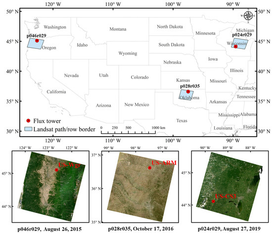
Figure 1.
The locations of three study areas (top) and corresponding Landsat 8 OLI true-color surface reflectance images (bottom), where the pxxxryyy indicates the path and row numbers.
2.2. Data
2.2.1. Collection 2 Landsat 8 Surface Reflectance and Temperature Data
The Landsat 8 Collection 2 Level 2 Science Product (L2SP) data were used. The Collection 2 data were released by the USGS Earth Resources Observation and Science (EROS) Center in 2020, with improved geometric accuracy and radiometric calibration compared with previous Collection 1 products [46]. A total of 15 Landsat 8 L2SP scenes with cloud cover <5% (Table 1) were downloaded. Landsat 8 L2SP data include 30 m surface reflectance (SR) and surface temperature (ST) bands derived from Landsat 8 Level-1 data, intermediate bands used in ST calculation and a Quality Assessment (QA) band, indicating the presence of cloud, cloud shadow and snow for each 30 m pixel [47]. The Landsat 8 SR is derived using an atmospheric correction software called Land Surface Reflectance Code (LaSRC) [48]. The Landsat 8 ST is derived using the MODTRAN radiative transfer model [49] with a single thermal band (band 10, 10.6–11.19 μm). We used the coastal/aerosol (0.43–0.45 μm), blue (0.45–0.51 μm), green (0.53–0.59 μm), red (0.64–0.67 μm), near infrared (NIR) (0.85–0.88 μm) and two shortwave infrared (SWIR) bands (1.57–1.75 μm and 2.11–2.29 μm) SR and the ST. The LaSRC surface reflectance has root mean squared error [48] of 11.0 × 10⁻³, 8.5 × 10⁻³, 5.4 × 10⁻³, 4.0 × 10⁻³, 2.6 × 10⁻³, 1.1 × 10⁻³ and 3.6 × 10⁻³ for the seven Landsat 8 bands when compared with the surface reflectance derived using the same 6S model but parameterized with ground-measured aerosols [48]. No independent validation of Landsat 8 ST has been found, while the validation of the Landsat 5 and 7 ST that was derived using the same algorithm shows an RMSE of 2.2 K [50] compared with the surface radiation budget network (SURFRAD) measurements.

Table 1.
The 15 Landsat 8 scenes and the corresponding MOD16A2 products for three study areas. The MOD16A2 is an 8-day composite and the starting date of the composite is shown.
2.2.2. Collection-6 MODIS ET Product (MOD16A2)
The MOD16A2 Collection 6 ET product was used for downscaling, which is an 8-day composite produced at a 500 m pixel resolution. MOD16A2 is produced based on the Penman–Monteith equation, with major inputs including meteorological data along with remotely sensed vegetation properties, albedo and land cover [13]. The pixel values for MOD16A2 ET are the sum of all eight days’ ET within the composite period (mm/8-days). In this study, the corresponding MOD16A2 of the Landsat image is defined when the middle dates of the 8-day MODIS composite period are closest to the Landsat image acquisition dates (Table 1). In an evaluation study of the MOD16A2 product using tower ET measurements for the 46 AmeriFlux eddy flux towers [13], the reported average daily ET bias is −0.02 mm/day, the average mean absolute error (MAE) is 0.31 mm/day and is 24.1% of the ET measurements.
2.2.3. Meteorological Data (AgERA5)
The AgERA5 dataset provides daily surface meteorological data for the period from 1979 to present at a spatial resolution of 0.1° (~10 km at the equator) grid. This dataset is based on hourly European Centre for Medium-Range Weather Forecasts (ECMWF) fifth generation atmospheric reanalysis (ERA5) data at surface level and is referred to as AgERA5 as it is tailored for users in the agricultural domain. The AgERA5 dataset is used as it is new and provides the highest spatial resolution among all the public available meteorological reanalysis datasets. Several recent studies have proved better performances of ERA5-derived climate parameters compared with other climate reanalysis datasets and satellite-derived and ground-observed climate parameters [51,52,53,54]. The dataset variables include temperature, precipitation, wind speed, snow thickness, humidity, cloud cover, radiation and vapor pressure [55]. The variables used in this study are shown in Table 2 and are available from Climate Data Store API (https://cds.climate.copernicus.eu/api-how-to (accessed on 3 September 2022)).
Table 2.
Descriptions of the sixteen Landsat 8 and sixteen AgERA5 variables.
2.2.4. AmeriFlux Eddy Covariance Flux Measurements
We used latent heat flux measured from eddy covariance flux towers in the AmeriFlux network to validate MODIS-downscaled ET. The AmeriFlux network (https://ameriflux.lbl.gov/ (accessed on 3 September 2022)) was established in 1996, providing standardized datasets of half-hourly to hourly carbon dioxide, water vapor and energy exchanges between terrestrial ecosystems and the atmosphere measured by eddy covariance across a diverse range of ecosystems and climates [56]. We selected three AmeriFlux sites (Section 2.1). The half-hourly latent heat flux (LE; W/m2) and air temperature (T; °C) measurements were used to estimate ET using the method in Mu et al., [13]. To be specific, the 8-day ET is generated by summing daily ET (mm/day) values for the 8-day interval with the same starting date as the MODIS ET product. The daily ET is calculated from the half-hourly ET (mm/30 min) as
where ET is the daily ET (mm/day), ETk is the kth half-hourly ET (mm/30 min) of the n reliable half-hourly ET and 48 indicates there are 48 half-hour periods in a day. The 30-min ET (mm/30 min) is calculated as:
where Tk and are air temperature in Celsius degree and latent heat flux, respectively, for the kth 30-min observation window and λ is the latent heat of vaporization (J/kg). The daily ET is calculated as (1) when the number of the reliable 30-min measurements (n) of both LE and T are no less than 40 and estimated by linear interpolation with the two nearest daily ET values otherwise.
3. Method
3.1. Thirty-Two Explanatory Variables
Thirty-two explanatory variables were used as input predictors to train the deep learning models, including sixteen Landsat 8 variables and sixteen AgERA5 meteorological variables. Specifically, Landsat 8 variables include seven band Landsat 8 1-7 SR and the ST, and eight spectral band indices related with vegetation greenness and water content, including Normalized Difference Vegetation Index (NDVI) [57], Enhanced Vegetation Index (EVI) [58], Soil Adjusted Vegetation Index (SAVI) [59], Modified Soil Adjusted Vegetation Index (MSAVI) [60], Normalized Difference Moisture Index (NDMI) [61], Normalized Difference Water Index (NDWI) [62], Temperature Vegetation Drought Index (TDVI) [63] and Normalized Difference Infrared Index-band 7 (NDIIb7) calculated from Landsat 8 band 1-7 SR and ST [64]. These indices related to vegetation, soil moisture and water status are contributing factors for ET and have been used for ET estimation [39,65]. Particularly, TVDI represents the water stress of vegetation [54], which was estimated using the triangular shape of ST and NDVI scatter plots using the equation in Table 2, where Ts is the Landsat 8 ST for each pixel, Tsmin is the minimum ST for a given NDVI (i.e., located in the wet edge in the ST-NDVI space) and Tsmax is the maximum ST for a given NDVI (i.e., located in the dry edge in the ST-NDVI space). The coefficients (a, b) are estimated using a linear regression between NDVI and the maximum ST for given NDVI values (i.e., the dry edge) and (c, d) are estimated using a linear regression between NDVI and the minimum ST for given NDVI values (i.e., the wet edge). Note that correction existing in these thirty-two explanatory variables (i.e., collinearity) should have little impact on the modeling capability of deep learning [66,67] and thus we include them to avoid missing important perdition variables.
AgERA5 meteorological variables include those related to wind speed, temperature, relative humidity, solar radiation and water vapor (Table 2), which are important for ET estimation.
3.2. DNN Regression Model
A Deep Neural Network (DNN) is an artificial neural network with multiple hidden layers between its inputs and outputs [68]. In this study, DNN is used for ET regression on the 32 explanatory variables (Section 3.1). Consequently, a 32-element array of the explanatory variables is used as the input layer and the MOD16A2 ET (one single value) as the output layer. Each hidden unit j of the hidden layer l is derived from all hidden units (or input layer values for the first layer) from the previous layer l − 1, as shown in Figure 2b:
where is the hidden unit value for unit j of layer l, is the weight from the hidden units , is the bias of the hidden unit and f is the nonlinear activation function. In this study, we choose the rectified linear unit (ReLU) nonlinear function as f(xj) [69] (Figure 2b).
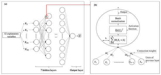
Figure 2.
The structure of the DNN regression model (a) and the logic process of value derivation of each unit in the layer (b).
The DNN training is to find optimal weights and bias coefficients for each layer to minimize a cost function that measures the discrepancy between MOD16A2 ET and the estimated ET with a Back Propagation (BP) procedure (i.e., conventional gradient descent algorithm) [70]. Given a fixed training set {(x(1), y(1)), …, (x(n), y(n))} with n training samples, the cost function to be minimized is defined by
where x(t) is the 32-element input vector and y(t) is the scalar output of a single ET value. To prevent overfitting, a regularization term is added to each hidden layer to alleviate severe gradient explosion in deep networks, which makes the training faster and more stable [71]. This study used the batch normalization as regularization [72].
The downscaled ET values were estimated with the trained DNN model. Our DNN regression model has 8 layers, including 7 hidden layers and 1 output layer as illustrated in Figure 2a. Specifically, the overall process includes the application of the ReLU activation function, which is followed by a batch normalization reducing overfitting. Batch normalization was applied after each hidden layer (Figure 2b). The 7 hidden layers have 256, 256, 256, 512, 512, 1024 and 1024 units, respectively. The mini batch gradient descent optimizer was used with a momentum value of 0.9 to find the optimal network coefficients and the mini-batch size was set as 64. The epoch number for training was 80. The learning rate was initialized as 0.01 and decreased 10 times whenever the loss function of an independent validation dataset stopped changing. The final decaying learning rate was fixed at 0.000001. The Python programming environment with TensorFlow and Keras libraries (https://keras.io/ (accessed on 3 September 2022)) were used to implement the DNN model training and application.
3.3. Spatial and Temporal Data Reconciliation for Training and Prediction
The DNN training is conducted using all the input and output variables at 500 m resolution, while the DNN prediction is conducted using the input variables at 30 m resolution. It implicitly assumes scale invariance of the relationship between the 32 input explanatory variables and the output ET. Such assumption has been used for many other downscaling applications, such as for surface reflectance [73,74], temperature [75], tree cover [76] and leaf area index [77]. A DNN model is trained for each study area and each Landsat image acquisition date so that spatially and temporally explicit DNN models are used to account the spatial and temporal variation. A 500 m pixel can be used for training only if the number of cloud-free Landsat pixels within the MODIS pixel extent is more than 30% and the MO16A2 ET is good quality according to MODIS ET_QC. The Landsat cloud-free is defined as absence of cloud, cloud shadow and snow using the Landsat quality assessment (QA) band.
The spatial and temporal resolution among the 32 explanatory variables and the MOD16A2 ET must be reconciled before training and prediction. The Landsat 8 variables from a single scene are used to represent the 8-day average surface conditions, assuming those surface states vary little in an 8-day period. However, meteorological variables change dramatically in an 8-day period. To handle such change, the daily meteorological variables are aggregated to an 8-day average and combined with MOD16A2 ET for training. In prediction, the Landsat 8 single-date surface variables are combined with the 8-day average meteorological variables to predict the 8-day average ET.
Spatial reconciliation is different for training and prediction, as they are conducted at different resolutions. For training, Landsat 8 is aggregated to a 500 m resolution using the simple area average method. Ideally, a more advanced aggregation method should be used to take into consideration the MODIS ET Point Spread Function (PSF) [78]. However, the PSF of the MODIS 8-day composite ET is difficult to characterize, as the MODIS image has a unique PSF for each acquisition date and each pixel in the 8-day period that is determined by the pixel-specific viewing zenith and azimuth angle on the acquisition date [78,79]. For prediction, the 30 m Landsat 8 variables are used directly as input. The AgERA5 meteorological variables were aggregated to the MODIS 500 m resolution for training and to the 30 m Landsat resolution for prediction using a non-linear spatial interpolation method proposed by [80].
3.4. Evaluation Methods
The evaluation is conducted in three different ways, each with different estimated and evaluated ET. First, the 500 m MODIS-based samples are randomly split into 80% for training and 20% for evaluation. The trained models are applied to the 20% evaluation samples to predict ET and compared with the MOD16A2 ET. Secondly, the estimated ET image at a 30 m resolution is aggregated to the 500 m resolution to compare with the 500 m MOD16A2 ET images (used as evaluation ET). Only good quality MOD16A2 ET values will be used for evaluation. Finally, the estimated ET at 30 m resolution is compared with the ET measured by the eddy covariance at the three AmeriFlux sites’ eddy (used as evaluation ET).
Several metrics were used to evaluate model performance, including the coefficients of determination (R2), root-mean-square deviation (RMSD) and relative RMSD (rRMSD, %).
where and refer to the evaluation (i.e., MODIS or eddy covariance observed ET) and the estimated ET, is the evaluation mean ET value and n is the total number of samples.
In addition, a Random Forest (RF) regression was used as a benchmark to evaluate the performance of the DNN regression model as it was often used for ET downscaling [24,81]. RF is a decision tree-based algorithm that combines several decision trees fitted in different random subsets of the training data [82]. Each tree is considered a weak learner; however, the combination of trees (ensemble) results in a single model with high predictive power [83]. There are many hyperparameters for training, but only one main hyperparameter (the number of trees) was tuned in this study. The number of trees was optimized to be 100. The RF workflow was implemented in Python programming language using the sklearn package.
4. Results
4.1. Evaluation Results for the 20% MOD16A2 Samples
Figure 3 shows the R2, RMSD and rRMSD comparisons of the 20% MOD16A2 evaluation samples between the random forest (in yellow) and the DNN regression model (in blue) from the three study regions. The numbers of the training samples are: 119,329, 84,984, 88,545, 99,620 and 98,539 for the five dates in the p046r029 study area; 50,559, 79,892, 81,060, 112,138, 99,397, 94,807 and 52,224 for the seven dates in the p028r035 study area; 118,100, 88,956 and 73,808 for the three dates in the p024r029 study area. All the results indicated that the DNN regression model has a higher R2 and lower RMSD and rRMSD (the average values: 0.67, 2.63 mm/8d and 14.25%, respectively) compared with the random forest model (0.64, 2.76 mm/8d and 14.92%, respectively), which signified that the proposed DNN regression model can more precisely predict ET than the random forest model. In the sparse vegetation region of p028r035, the DNN regression model has the highest R2 (ranging from 0.66 to 0.84) and lowest RMSD (0.31 to 2.89 mm/8d) and rRMSD (4.85% to 14.59%), and the corresponding values for the random forest model are 0.64 to 0.82, 0.33 to 3.04 mm/8d and 5.21% to 15.33%, respectively. At the same time, this region witnessed the smallest improvement using the DNN regression model. In contrast, the vegetated region of p024r029 has the lowest R2 (0.35 to 0.75) and the highest RMSD (3.11 to 5.97 mm/8d) with the DNN regression model, and values from the random forest model are 0.31 to 0.72 and 3.29 to 6.26 mm/8d, respectively.
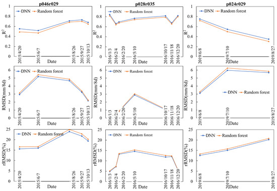
Figure 3.
R2 (top row), RMSD (middle row) and rRMSD (%, bottom row) for the 20% MOD16A2 evaluation samples for the random forest (in yellow) and DNN model (in blue) in three study areas (three different columns).
4.2. Evaluation against MOD16A2 ET Images
4.2.1. Visual Evaluation at the 30 m Scale
Figure 4, Figure 5 and Figure 6 show Landsat 8 true-color SR images (first row), MOD16A2 ET (second row), random forest downscaled 30 m ET (third row) and DNN downscaled 30 m ET (fourth row). The results are shown for the p046r029 (Figure 4), p028r035 (Figure 5) and p024r029 (Figure 6) study regions, respectively, and the two zoom-in example areas are also shown in the second and third columns. Both the random forest downscaled ET (third row) and the DNN downscaled ET (fourth row) showed more spatial details than the MOD16A2 ET (second row), and the 30 m downscaled ET has more evident dependence on land-cover type, e.g., the crop field shape can be seen in the downscaled ET. However, there are visual differences between the random forest and the DNN downscaled ET, especially in the zoomed-in figures. The DNN downscaled ET map appears more consistent with the Landsat 8 true-color images in spatial details and has a larger dynamic ET range than the random forest downscaled ET.
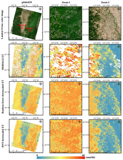
Figure 4.
The p046r029 region Landsat 8 true-color SR images (first row), MOD16A2 ET (second row), random forest downscaled ET (third row) and DNN downscaled ET (fourth row). Two zoom-in areas are shown in the second and third columns. The Landsat image was acquired on 25 August 2015. The white pixels in the MOD16A2 map indicate fill values.
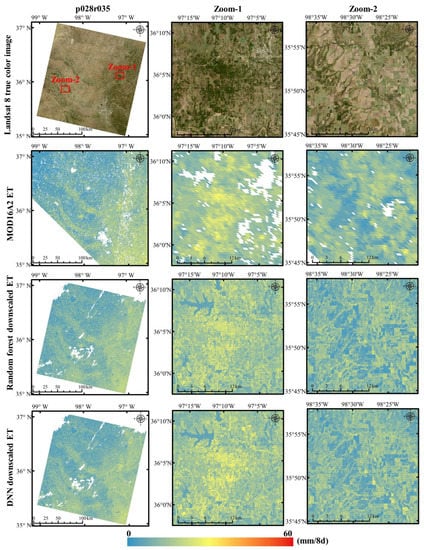
Figure 5.
Same as Figure 4 but for the p028r035 region with Landsat 8 image acquired on 17 October 2016.
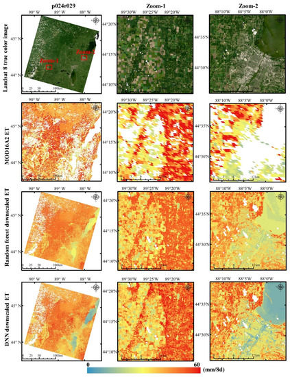
Figure 6.
Same as Figure 4 but for the p024r029 region with Landsat 8 image acquired on 27 August 2019.
4.2.2. Metric Evaluation at the 500 m Scale
Figure 7 shows the scatterplots of MOD16A2 500 m ET against the downscaled ET aggregated to 500 m, estimated using the random forest model (top row) and DNN model (bottom row) for the three study regions. All images for each study area in Table 1 are considered and only good quality 500 m MODIS ET values are considered. The aggregated downscaled ET using the DNN model has higher R2 (ranging from 0.73 to 0.94), lower RMSD (1.48 to 5.88 mm/8d) and rRMSD (16.36% to 22.30%) values than the random forest model (R2: 0.71 to 0.94, RMSD: 1.55 to 6.13 mm/8d and rRMSD: 17.17% to 23.35%, respectively) in all three study regions. It is evident that the DNN ET and MOD16A2 ET is closer to a 1:1 line and less scattered than the random forest ET and MOD16A2 ET. These results indicate that the proposed DNN model can make the downscaled ET more consistent with MOD16A2 than the random forest model.
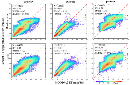
Figure 7.
Scatterplots of MOD16A2 500 m good quality ET against the downscaled ET aggregated to 500 m, estimated using the random forest (top row) and the DNN model (bottom row) for three study regions. For each study region, all the Landsat images shown in Table 1 are considered.
4.3. Evaluation against AmeriFlux Eddy Covariance Flux Measurements
Table 3 shows 8-day ET comparisons between AmeriFlux in situ observations and the three different satellite derived ET, i.e., the RF downscaled ET (30 m), the DNN downscaled ET (30 m) and MOD16A2 ET (500 m) for the three AmeriFlux sites (US-Wgr, US-ARM and US-CS3). The three sites were combined in order to drive a statistically meaningful comparison, as there are a limited number of ET values at each site location. Results indicated the DNN downscaled ET has the better consistency with the in situ observations. The number of matched MOD16A2 ET values are smaller than the number of matched DNN downscaled ET values because of the apparent missing high-quality data in MOD16A2 ET (Figure 4, Figure 5 and Figure 6).
Table 3.
Evaluation metrics against three AmeriFlux in situ ET (mm/8-days) for the RF downscaled ET (30 m), DNN downscaled ET (30 m) and MOD16A2 ET (500 m).
5. Discussion
ET estimation from remote sensing images can provide high-spatial coverage but is also complicated by the nonlinear, dynamic and complex relationship. The MODIS ET has been widely used, but a higher resolution ET map is needed for agricultural applications. This study constructs a DNN model to downscale MOD16A2 ET to a Landsat resolution by incorporating Landsat and meteorological data. Results showed that the downscaled ET is visually consistent with MOD16A2 ET on a large scale but captured more spatial details. The DNN model had a higher R2 and lower RMSD than the random forest model. This is expected, since deep learning is able to extract informative features with multiple levels of representation from lower primitive levels to higher abstract levels [31,84]. Random forest regression has a lower accuracy and lower variation in the estimated ET values, because random forest regression tends to overestimate low values but underestimates high values [35]. The downscaled ET also showed higher consistency with the in situ flux tower ET than the 500 m MOD16A2 (Figure 8). However, the US-ARM site ET was 6.4 mm/8d in the 8–16 May 2016 8-day period, but the corresponding MOD16A2 and the downscaled ET were 18.2 mm/8d and 20.6 mm/8d, respectively. This difference in the US-ARM site possibly results from the heterogeneous land covers within the MODIS pixel area that include small patches of winter wheat, maize, soybean and sorghum (Figure 8). It is known that the footprint of the flux tower is not fixed and varies with meteorological conditions [85], and heterogeneous land surface within a targeted area (e.g., a MODIS pixel) may reduce the spatial representativeness of the targeted area to the flux footprint. In addition, the underestimation of the AmeriFlux data, a frequently observed phenomenon because of non-closure of the surface energy balance for ET field measurements collected by the eddy-covariance method [86,87], likely contributes to this difference.
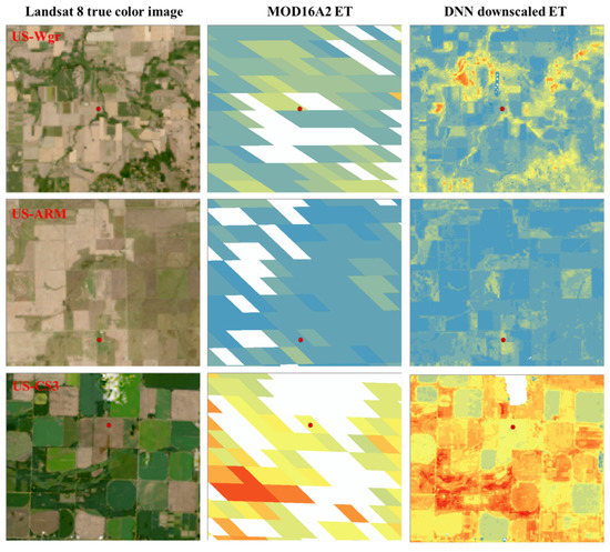
Figure 8.
Landsat 8 true-color SR images (first column), MOD16A2 ET (second column) and DNN downscaled ET (third column) near three flux towers on the three Landsat acquisition dates from Figure 1.
ET calculation is typically based on physical principles that conserve either energy or mass, or both. This study combined remotely sensed variables (e.g., ST and VI) with concurrent meteorological measurements (e.g., maximum and minimum air temperature, relative humidity, solar radiation and wind speed) as predictor variables. The meteorological data are used as they are important parameters for ET calculation, e.g., in physical models such as SEBAL [10,11], SEBS [88] and REBM [89]. We aggregated the hourly meteorological data into 8-day periods to match the 8-day composite period of the MOD16A2 data. Aggregation (from high resolution to low resolution) usually has much better accuracy than resampling from low resolution to high resolution. However, the spatial scale of meteorological data in this study is 0.1° (~10 km at the equator), which limited its applicability in the heterogeneous region compared with high-spatial resolution satellite images. A more advanced spatial-interpolation method to increase spatial resolutions of meteorological data should be further explored [90,91].
There are some limitations for the applications of the DNN downscaled ET. First, MODIS ET were used as training data and the accuracy of the trained model is limited by the accuracy of MODIS ET, i.e., with 25% uncertainties [13]. Some better ET products at coarse resolution have been developed, with improved algorithms [92,93] or fusion models [40,94,95]. This study used the MOD16A2 product due to its wide application and easy access, but future study using more accurate ET products as training data is encouraged. Second, the downscaled 30 m ET map will have a lower temporal resolution than the MODIS data due to the 16-day revisit cycle. This could be addressed in two different ways in future work. On the one hand, the Landsat 8 in combination with Landsat 9, Sentinel-2A and Sentienl-2B will enable <2-day revisit cycle globally. The application of the method for Landsat 9 is straightforward, since the Landsat 9 bears the same sensor and the same bands and the data are processed into Collection-2 SR and ST once available [96]. Application of the proposed method to Sentinel-2 is more challenging, as it does not have thermal bands to derive ST. On the other hand, the clear-sky Landsat images with the high-spatial–temporal resolution can be generated by spatio-temporal fusion methods such as STARFM [97], ESTARFM [98] and FSDAF [99].
6. Conclusions
Accurate land surface evapotranspiration estimation is crucial to understand the hydrological cycle and energy budgets within terrestrial ecosystems [1,100]. In particular, the small patch agricultural fields require accurate temporal–spatial ET data to evaluate water requirement, to control water usage and to assess drought impact [4,5]. To this end, this study developed a DNN-based ET downscaling framework to improve the resolution of MODIS ET (MOD16A2). We first trained a DNN regression model on the MODIS resolution using the MOD16A2 data as a single response variable and the 32 Landsat 8 and meteorological variables aggregated/resampled to the MODIS resolution as explanatory variables. The DNN-downscaled ET was evaluated over three study areas and compared with the traditional random forest model. Results showed that the DNN regression model has higher R2 and lower RMSD and rRMSD (the average values: 0.67, 2.63 mm/8d and 14.25%, respectively) compared with the random forest model (0.64, 2.76 mm/8d and 14.92%, respectively) when evaluated on the independent samples. The spatial details were enhanced both in the DNN- and the random forest-downscaled ET, but the DNN-downscaled ET preserved more spatial variation and resembled more the land surface distribution. The two downscaled ET were degraded to the MODIS resolution and statistically compared with the MOD16A2. Results indicated that the downscaled ET from the DNN model has higher R2 (ranging from 0.727 to 0.943), lower RMSD (1.475 to 5.884 mm/8d) and rRMSD (16.36% to 22.30%) values compared with the random forest model (R2: 0.709 to 0.939, RMSD: 1.548 to 6.128 mm/8d and rRMSD: 17.17% to 23.35%, respectively) in all three study regions. The comparisons with in situ data from the flux towers showed that the downscaled ET has higher R2 and lower RMSD compared with MOD16A2. All the results showed that the proposed DNN model is promising to build Landsat ET records for land surface ET monitoring.
Author Contributions
Conceptualization, H.K.Z.; data curation, X.C. and Q.S.; funding acquisition, X.C.; investigation, H.K.Z.; methodology, X.C. and H.K.Z.; project administration, J.L.; supervision, J.L.; validation, X.C.; writing—original draft, X.C.; writing—review and editing, H.K.Z. and Z.O. All authors have read and agreed to the published version of the manuscript.
Funding
Xianghong Che, Qing Sun and Jiping Liu were supported by National Natural Science Foundation of China programs (Grant No. 41901379 and 42001310).
Conflicts of Interest
The authors declare that they have no known competing financial interest or personal relationships that could have appeared to influence the work reported in this paper.
References
- Fisher, J.B.; Melton, F.; Middleton, E.; Hain, C.; Anderson, M.; Allen, R.; McCabe, M.F.; Hook, S.; Baldocchi, D.; Townsend, P.A. The future of evapotranspiration: Global requirements for ecosystem functioning, carbon and climate feedbacks, agricultural management, and water resources. Water Resour. Res. 2017, 53, 2618–2626. [Google Scholar] [CrossRef]
- Shiri, J.; Sadraddini, A.A.; Nazemi, A.H.; Kisi, O.; Marti, P.; Fard, A.F.; Landeras, G. Evaluation of different data management scenarios for estimating daily reference evapotranspiration. Hydrol. Res. 2013, 44, 1058–1070. [Google Scholar] [CrossRef]
- Anderson, M.C.; Allen, R.G.; Morse, A.; Kustas, W.P. Use of Landsat thermal imagery in monitoring evapotranspiration and managing water resources. Remote Sens. Environ. 2012, 122, 50–65. [Google Scholar] [CrossRef]
- Diak, G.R.; Mecikalski, J.R.; Anderson, M.C.; Norman, J.M.; Kustas, W.P.; Torn, R.D.; DeWolf, R.L. Estimating land surface energy budgets from space: Review and current efforts at the University of Wisconsin—Madison and USDA–ARS. Bull. Am. Meteorol. Soc. 2004, 85, 65–78. [Google Scholar] [CrossRef]
- Zipper, S.C.; Loheide II, S.P. Using evapotranspiration to assess drought sensitivity on a subfield scale with HRMET, a high resolution surface energy balance model. Agric. For. Meteorol. 2014, 197, 91–102. [Google Scholar] [CrossRef]
- Jiang, L.; Islam, S. Estimation of surface evaporation map over southern Great Plains using remote sensing data. Water Resour. Res. 2001, 37, 329–340. [Google Scholar] [CrossRef]
- Wang, K.; Li, Z.; Cribb, M. Estimation of evaporative fraction from a combination of day and night land surface temperatures and NDVI: A new method to determine the Priestley–Taylor parameter. Remote Sens. Environ. 2006, 102, 293–305. [Google Scholar] [CrossRef]
- Allen, R.G.; Tasumi, M.; Morse, A.; Trezza, R.; Wright, J.L.; Bastiaanssen, W.; Kramber, W.; Lorite, I.; Robison, C.W. Satellite-based energy balance for mapping evapotranspiration with internalized calibration (METRIC)—Applications. J. Irrig. Drain. Eng. 2007, 133, 395–406. [Google Scholar] [CrossRef]
- Allen, R.G.; Tasumi, M.; Trezza, R. Satellite-based energy balance for mapping evapotranspiration with internalized calibration (METRIC)—Model. J. Irrig. Drain. Eng. 2007, 133, 380–394. [Google Scholar] [CrossRef]
- Bastiaanssen, W.G.; Menenti, M.; Feddes, R.; Holtslag, A. A remote sensing surface energy balance algorithm for land (SEBAL). 1. Formulation. J. Hydrol. 1998, 212, 198–212. [Google Scholar] [CrossRef]
- Bastiaanssen, W.G.; Pelgrum, H.; Wang, J.; Ma, Y.; Moreno, J.; Roerink, G.; Van der Wal, T. A remote sensing surface energy balance algorithm for land (SEBAL). Part 2: Validation. J. Hydrol. 1998, 212, 213–229. [Google Scholar] [CrossRef]
- Norman, J.; Anderson, M.; Kustas, W.; French, A.; Mecikalski, J.; Torn, R.; Diak, G.; Schmugge, T.; Tanner, B. Remote sensing of surface energy fluxes at 101-m pixel resolutions. Water Resour. Res. 2003, 39. [Google Scholar] [CrossRef]
- Mu, Q.; Zhao, M.; Running, S.W. Improvements to a MODIS global terrestrial evapotranspiration algorithm. Remote Sens. Environ. 2011, 115, 1781–1800. [Google Scholar] [CrossRef]
- Wang, K.; Dickinson, R.E.; Wild, M.; Liang, S. Evidence for decadal variation in global terrestrial evapotranspiration between 1982 and 2002: 1. Model development. J. Geophys. Res. Atmos. 2010, 115. [Google Scholar] [CrossRef]
- Fisher, J.B.; Tu, K.P.; Baldocchi, D.D. Global estimates of the land–atmosphere water flux based on monthly AVHRR and ISLSCP-II data, validated at 16 FLUXNET sites. Remote Sens. Environ. 2008, 112, 901–919. [Google Scholar] [CrossRef]
- Fritz, S.; See, L.; McCallum, I.; You, L.; Bun, A.; Moltchanova, E.; Duerauer, M.; Albrecht, F.; Schill, C.; Perger, C. Mapping global cropland and field size. Glob. Change Biol. 2015, 21, 1980–1992. [Google Scholar] [CrossRef]
- Melton, F.S.; Huntington, J.; Grimm, R.; Herring, J.; Hall, M.; Rollison, D.; Erickson, T.; Allen, R.; Anderson, M.; Fisher, J.B. OpenET: Filling a critical data gap in water management for the western united states. J. Am. Water Resour. Assoc. 2021, 1–24. [Google Scholar] [CrossRef]
- Dwyer, J.L.; Roy, D.P.; Sauer, B.; Jenkerson, C.B.; Zhang, H.K.; Lymburner, L. Analysis ready data: Enabling analysis of the Landsat archive. Remote Sens. 2018, 10, 1363. [Google Scholar] [CrossRef]
- Anderson, M.C.; Kustas, W.P.; Alfieri, J.G.; Gao, F.; Hain, C.; Prueger, J.H.; Evett, S.; Colaizzi, P.; Howell, T.; Chávez, J.L. Mapping daily evapotranspiration at Landsat spatial scales during the BEAREX’08 field campaign. Adv. Water Resour. 2012, 50, 162–177. [Google Scholar] [CrossRef]
- Bhattarai, N.; Quackenbush, L.J.; Dougherty, M.; Marzen, L.J. A simple Landsat–MODIS fusion approach for monitoring seasonal evapotranspiration at 30 m spatial resolution. Int. J. Remote Sens. 2015, 36, 115–143. [Google Scholar] [CrossRef]
- Cammalleri, C.; Anderson, M.; Gao, F.; Hain, C.; Kustas, W. A data fusion approach for mapping daily evapotranspiration at field scale. Water Resour. Res. 2013, 49, 4672–4686. [Google Scholar] [CrossRef]
- Cammalleri, C.; Anderson, M.; Gao, F.; Hain, C.; Kustas, W. Mapping daily evapotranspiration at field scales over rainfed and irrigated agricultural areas using remote sensing data fusion. Agric. For. Meteorol. 2014, 186, 1–11. [Google Scholar] [CrossRef]
- Hong, S.-h.; Hendrickx, J.M.; Borchers, B. Down-scaling of SEBAL derived evapotranspiration maps from MODIS (250 m) to Landsat (30 m) scales. Int. J. Remote Sens. 2011, 32, 6457–6477. [Google Scholar] [CrossRef]
- Ke, Y.; Im, J.; Park, S.; Gong, H. Spatiotemporal downscaling approaches for monitoring 8-day 30 m actual evapotranspiration. ISPRS J. Photogramm. Remote Sens. 2017, 126, 79–93. [Google Scholar] [CrossRef]
- Semmens, K.A.; Anderson, M.C.; Kustas, W.P.; Gao, F.; Alfieri, J.G.; McKee, L.; Prueger, J.H.; Hain, C.R.; Cammalleri, C.; Yang, Y. Monitoring daily evapotranspiration over two California vineyards using Landsat 8 in a multi-sensor data fusion approach. Remote Sens. Environ. 2016, 185, 155–170. [Google Scholar] [CrossRef]
- Singh, R.K.; Senay, G.B.; Velpuri, N.M.; Bohms, S.; Verdin, J.P. On the downscaling of actual evapotranspiration maps based on combination of MODIS and Landsat-based actual evapotranspiration estimates. Remote Sens. 2014, 6, 10483–10509. [Google Scholar] [CrossRef]
- Wang, T.; Tang, R.; Li, Z.-L.; Jiang, Y.; Liu, M.; Niu, L. An improved spatio-temporal adaptive data fusion algorithm for evapotranspiration mapping. Remote Sens. 2019, 11, 761. [Google Scholar] [CrossRef]
- Zhang, L.; Yao, Y.; Bei, X.; Li, Y.; Shang, K.; Yang, J.; Guo, X.; Yu, R.; Xie, Z. ERTFM: An Effective Model to Fuse Chinese GF-1 and MODIS Reflectance Data for Terrestrial Latent Heat Flux Estimation. Remote Sens. 2021, 13, 3703. [Google Scholar] [CrossRef]
- Liu, Y.; Zhang, S.; Zhang, J.; Tang, L.; Bai, Y. Assessment and comparison of six machine learning models in estimating evapotranspiration over croplands using remote sensing and meteorological factors. Remote Sens. 2021, 13, 3838. [Google Scholar] [CrossRef]
- Bengio, Y.; Courville, A.; Vincent, P. Representation learning: A review and new perspectives. IEEE Trans. Pattern Anal. Mach. Intell. 2013, 35, 1798–1828. [Google Scholar] [CrossRef]
- LeCun, Y.; Bengio, Y.; Hinton, G. Deep learning. Nature 2015, 521, 436–444. [Google Scholar] [CrossRef]
- Marçais, J.; de Dreuzy, J.R. Prospective interest of deep learning for hydrological inference. Groundwater 2017, 55, 688–692. [Google Scholar] [CrossRef] [PubMed]
- Shen, C.; Laloy, E.; Elshorbagy, A.; Albert, A.; Bales, J.; Chang, F.-J.; Ganguly, S.; Hsu, K.-L.; Kifer, D.; Fang, Z. HESS Opinions: Incubating deep-learning-powered hydrologic science advances as a community. Hydrol. Earth Syst. Sci. 2018, 22, 5639–5656. [Google Scholar] [CrossRef]
- Di Noia, A.; Hasekamp, O.P. Neural Networks and Support Vector Machines and Their Application to Aerosol and Cloud Remote Sensing: A Review. In Springer Series in Light Scattering; Kokhanovsky, A., Ed.; Springer: Cham, Switzerland, 2018. [Google Scholar] [CrossRef]
- She, L.; Zhang, H.K.; Li, Z.; de Leeuw, G.; Huang, B. Himawari-8 Aerosol Optical Depth (AOD) Retrieval Using a Deep Neural Network Trained Using AERONET Observations. Remote Sens. 2020, 12, 4125. [Google Scholar] [CrossRef]
- Chen, Z.; Zhu, Z.; Jiang, H.; Sun, S. Estimating Daily Reference Evapotranspiration Based on Limited Meteorological Data Using Deep Learning and Classical Machine Learning Methods. J. Hydrol. 2020, 591, 125286. [Google Scholar] [CrossRef]
- Ferreira, L.B.; da Cunha, F.F. New approach to estimate daily reference evapotranspiration based on hourly temperature and relative humidity using machine learning and deep learning. Agric. Water Manag. 2020, 234, 106113. [Google Scholar] [CrossRef]
- Cui, Y.; Song, L.; Fan, W. Generation of spatio-temporally continuous evapotranspiration and its components by coupling a two-source energy balance model and a deep neural network over the Heihe River Basin. J. Hydrol. 2021, 597, 126176. [Google Scholar] [CrossRef]
- Carter, C.; Liang, S. Evaluation of ten machine learning methods for estimating terrestrial evapotranspiration from remote sensing. Int. J. Appl. Earth Obs. Geoinf. 2019, 78, 86–92. [Google Scholar] [CrossRef]
- Shang, K.; Yao, Y.; Liang, S.; Zhang, Y.; Fisher, J.B.; Chen, J.; Liu, S.; Xu, Z.; Zhang, Y.; Jia, K. DNN-MET: A deep neural networks method to integrate satellite-derived evapotranspiration products, eddy covariance observations and ancillary information. Agric. For. Meteorol. 2021, 308, 108582. [Google Scholar] [CrossRef]
- Kottek, M.; Grieser, J.; Beck, C.; Rudolf, B.; Rubel, F. World map of the Köppen-Geiger climate classification updated. Meteorol. Z. 2006, 15, 259–263. [Google Scholar] [CrossRef]
- Schmidt, A.; Law, B. AmeriFlux US-Wgr Willamette Grass; Lawrence Berkeley National Lab. (LBNL): Berkeley, CA, USA, 2019.
- Mullens, T.J. Evaluation and Improvements of the Offline CLM4 Using ARM Data. Master’s Thesis, San Jose State University, San Jose, CA, USA, 2013. [Google Scholar]
- Lokupitiya, E.; Denning, S.; Paustian, K.; Baker, I.; Schaefer, K.; Verma, S.; Meyers, T.; Bernacchi, C.; Suyker, A.; Fischer, M. Incorporation of crop phenology in Simple Biosphere Model (SiBcrop) to improve land-atmosphere carbon exchanges from croplands. Biogeosciences 2009, 6, 969–986. [Google Scholar] [CrossRef]
- Desai, A. AmeriFlux US-CS3 Central Sands Irrigated Agricultural Field; Lawrence Berkeley National Lab. (LBNL): Berkeley, CA, USA, 2020.
- Landsat 8-9 Collection 2 (C2) Level 2 Science Product (L2SP) Guide; United States Geological Survey: Asheville, NC, USA, 2022; pp. 1–42.
- Foga, S.C.; Scaramuzza, P.L.; Guo, S.; Zhu, Z.; Dilley, R.D.; Beckmann, T.; Schmidt, G.L.; Dwyer, J.L.; Hughes, M.J.; Laue, B. Cloud detection algorithm comparison and validation for operational Landsat data products. Remote Sens. Environ. 2017, 194, 379–390. [Google Scholar] [CrossRef]
- Vermote, E.; Justice, C.; Claverie, M.; Franch, B. Preliminary analysis of the performance of the Landsat 8/OLI land surface reflectance product. Remote Sens. Environ. 2016, 185, 46–56. [Google Scholar] [CrossRef] [PubMed]
- Cook, M.; Schott, J.R.; Mandel, J.; Raqueno, N. Development of an operational calibration methodology for the Landsat thermal data archive and initial testing of the atmospheric compensation component of a Land Surface Temperature (LST) product from the archive. Remote Sens. 2014, 6, 11244–11266. [Google Scholar] [CrossRef]
- Malakar, N.K.; Hulley, G.C.; Hook, S.J.; Laraby, K.; Cook, M.; Schott, J.R. An operational land surface temperature product for Landsat thermal data: Methodology and validation. IEEE Trans. Geosci. Remote Sens. 2018, 56, 5717–5735. [Google Scholar] [CrossRef]
- Nogueira, M. Inter-comparison of ERA-5, ERA-interim and GPCP rainfall over the last 40 years: Process-based analysis of systematic and random differences. J. Hydrol. 2020, 583, 124632. [Google Scholar] [CrossRef]
- Tarek, M.; Brissette, F.P.; Arsenault, R. Evaluation of the ERA5 reanalysis as a potential reference dataset for hydrological modelling over North America. Hydrol. Earth Syst. Sci. 2020, 24, 2527–2544. [Google Scholar] [CrossRef]
- Belmonte Rivas, M.; Stoffelen, A. Characterizing ERA-Interim and ERA5 surface wind biases using ASCAT. Ocean Sci. 2019, 15, 831–852. [Google Scholar] [CrossRef]
- Zhou, Q.; Ismaeel, A. Seasonal Cropland Trends and Their Nexus with Agrometeorological Parameters in the Indus River Plain. Remote Sens. 2020, 13, 41. [Google Scholar] [CrossRef]
- Boogaard, H.; Schubert, J.; De Wit, A.; Lazebnik, J.; Hutjes, R.; Van der Grijn, G. Agrometeorological Indicators from 1979 to Present Derived from Reanalysis, Version 1.0; Copernicus Climate Change Service (C3S) Climate Data Store (CDS): Brussels, Belgium, 2020. [Google Scholar] [CrossRef]
- Baldocchi, D. ‘Breathing’of the terrestrial biosphere: Lessons learned from a global network of carbon dioxide flux measurement systems. Aust. J. Bot. 2008, 56, 1–26. [Google Scholar] [CrossRef]
- Tucker, C.J. Red and photographic infrared linear combinations for monitoring vegetation. Remote Sens. Environ. 1979, 8, 127–150. [Google Scholar] [CrossRef]
- Huete, A.; Didan, K.; Miura, T.; Rodriguez, E.P.; Gao, X.; Ferreira, L.G. Overview of the radiometric and biophysical performance of the MODIS vegetation indices. Remote Sens. Environ. 2002, 83, 195–213. [Google Scholar] [CrossRef]
- Huete, A.R. A soil-adjusted vegetation index (SAVI). Remote Sens. Environ. 1988, 25, 295–309. [Google Scholar] [CrossRef]
- Qi, J.; Chehbouni, A.; Huete, A.R.; Kerr, Y.H.; Sorooshian, S. A modified soil adjusted vegetation index. Remote Sens. Environ. 1994, 48, 119–126. [Google Scholar] [CrossRef]
- Wilson, E.H.; Sader, S.A. Detection of forest harvest type using multiple dates of Landsat TM imagery. Remote Sens. Environ. 2002, 80, 385–396. [Google Scholar] [CrossRef]
- McFeeters, S.K. The use of the Normalized Difference Water Index (NDWI) in the delineation of open water features. Int. J. Remote Sens. 1996, 17, 1425–1432. [Google Scholar] [CrossRef]
- Sandholt, I.; Rasmussen, K.; Andersen, J. A simple interpretation of the surface temperature/vegetation index space for assessment of surface moisture status. Remote Sens. Environ. 2002, 79, 213–224. [Google Scholar] [CrossRef]
- Hunt, E.R., Jr.; Rock, B.N. Detection of changes in leaf water content using near-and middle-infrared reflectances. Remote Sens. Environ. 1989, 30, 43–54. [Google Scholar] [CrossRef]
- Yinghai, K.; Jungho, I.; Seonyoung, P.; Huili, G. Downscaling of MODIS One Kilometer Evapotranspiration Using Landsat-8 Data and Machine Learning Approaches. Remote Sens. 2016, 8, 215. [Google Scholar]
- Huang, F.; Zhang, J.; Zhou, C.; Wang, Y.; Huang, J.; Zhu, L. A deep learning algorithm using a fully connected sparse autoencoder neural network for landslide susceptibility prediction. Landslides 2020, 17, 217–229. [Google Scholar] [CrossRef]
- Levy, J.J.; Titus, A.J.; Petersen, C.L.; Chen, Y.; Salas, L.A.; Christensen, B.C. MethylNet: An automated and modular deep learning approach for DNA methylation analysis. BMC Bioinform. 2020, 21, 1–15. [Google Scholar] [CrossRef]
- Hinton, G.; Deng, L.; Yu, D.; Dahl, G.E.; Mohamed, A.-R.; Jaitly, N.; Senior, A.; Vanhoucke, V.; Nguyen, P.; Sainath, T.N. Deep neural networks for acoustic modeling in speech recognition: The shared views of four research groups. IEEE Signal Process. Mag. 2012, 29, 82–97. [Google Scholar] [CrossRef]
- Glorot, X.; Bordes, A.; Bengio, Y. Deep sparse rectifier neural networks. In Proceedings of the Fourteenth InterNational Conference on Artificial Intelligence and Statistics, Fort Lauderdale, FL, USA, 11–13 April 2011; pp. 315–323. [Google Scholar]
- Ruder, S. An overview of gradient descent optimization algorithms. arXiv 2016, arXiv:1609.04747. [Google Scholar]
- Bourlard, H.A.; Morgan, N. Connectionist Speech Recognition: A Hybrid Approach; Springer Science & Business Media: Berlin/Heidelberg, Germany, 2012; Volume 247. [Google Scholar]
- Ioffe, S.; Szegedy, C. Batch normalization: Accelerating deep network training by reducing internal covariate shift. In Proceedings of the International Conference on Machine Learning, Lille, France, 6–11 July 2015; pp. 448–456. [Google Scholar]
- Gao, F.; Masek, J.G.; Wolfe, R.E.; Huang, C. Building a consistent medium resolution satellite data set using moderate resolution imaging spectroradiometer products as reference. J. Appl. Remote Sens. 2010, 4, 043526. [Google Scholar]
- Zhang, H.K.; Huang, B.; Zhang, M.; Cao, K.; Yu, L. A generalization of spatial and temporal fusion methods for remotely sensed surface parameters. Int. J. Remote Sens. 2015, 36, 4411–4445. [Google Scholar] [CrossRef]
- Agam, N.; Kustas, W.P.; Anderson, M.C.; Li, F.; Colaizzi, P.D. Utility of thermal sharpening over Texas high plains irrigated agricultural fields. J. Geophys. Res. Atmos. 2007, 112. [Google Scholar] [CrossRef]
- Sexton, J.O.; Song, X.-P.; Feng, M.; Noojipady, P.; Anand, A.; Huang, C.; Kim, D.-H.; Collins, K.M.; Channan, S.; DiMiceli, C. Global, 30-m resolution continuous fields of tree cover: Landsat-based rescaling of MODIS vegetation continuous fields with lidar-based estimates of error. Int. J. Digit. Earth 2013, 6, 427–448. [Google Scholar] [CrossRef]
- Sun, L.; Gao, F.; Anderson, M.C.; Kustas, W.P.; Alsina, M.M.; Sanchez, L.; Sams, B.; McKee, L.; Dulaney, W.; White, W.A. Daily mapping of 30 m LAI and NDVI for grape yield prediction in California vineyards. Remote Sens. 2017, 9, 317. [Google Scholar] [CrossRef]
- Che, X.; Zhang, H.K.; Liu, J. Making Landsat 5, 7 and 8 reflectance consistent using MODIS nadir-BRDF adjusted reflectance as reference. Remote Sens. Environ. 2021, 262, 112517. [Google Scholar] [CrossRef]
- Xin, Q.; Olofsson, P.; Zhu, Z.; Tan, B.; Woodcock, C.E. Toward near real-time monitoring of forest disturbance by fusion of MODIS and Landsat data. Remote Sens. Environ. 2013, 135, 234–247. [Google Scholar] [CrossRef]
- Zhao, M.; Heinsch, F.A.; Nemani, R.R.; Running, S.W. Improvements of the MODIS terrestrial gross and net primary production global data set. Remote Sens. Environ. 2005, 95, 164–176. [Google Scholar] [CrossRef]
- Barrios, J.M.; Ghilain, N.; Arboleda, A.; Gellens-Meulenberghs, F. Daily evapotranspiration at sub-kilometre resolution through surface energy balance modelling and Random Forest-based downscaling. Geophys. Res. Abstr. 2019, 21, 1. [Google Scholar]
- Breiman, L. Random forests. Mach. Learn. 2001, 45, 5–32. [Google Scholar] [CrossRef]
- Huang, G.; Wu, L.; Ma, X.; Zhang, W.; Fan, J.; Yu, X.; Zeng, W.; Zhou, H. Evaluation of CatBoost method for prediction of reference evapotranspiration in humid regions. J. Hydrol. 2019, 574, 1029–1041. [Google Scholar] [CrossRef]
- Schmidhuber, J. Deep learning in neural networks: An overview. Neural Netw. 2015, 61, 85–117. [Google Scholar] [CrossRef] [PubMed]
- Chu, H.; Luo, X.; Ouyang, Z.; Chan, W.S.; Dengel, S.; Biraud, S.C.; Torn, M.S.; Metzger, S.; Kumar, J.; Arain, M.A. Representativeness of Eddy-Covariance flux footprints for areas surrounding AmeriFlux sites. Agric. For. Meteorol. 2021, 301, 108350. [Google Scholar] [CrossRef]
- Wang, K.; Dickinson, R.E. A review of global terrestrial evapotranspiration: Observation, modeling, climatology, and climatic variability. Rev. Geophys. 2012, 50. [Google Scholar] [CrossRef]
- Mauder, M.; Genzel, S.; Fu, J.; Kiese, R.; Soltani, M.; Steinbrecher, R.; Zeeman, M.; Banerjee, T.; De Roo, F.; Kunstmann, H. Evaluation of energy balance closure adjustment methods by independent evapotranspiration estimates from lysimeters and hydrological simulations. Hydrol. Process. 2018, 32, 39–50. [Google Scholar] [CrossRef]
- Su, Z. The Surface Energy Balance System (SEBS) for estimation of turbulent heat fluxes. Hydrol. Earth Syst. Sci. 2002, 6, 85–100. [Google Scholar] [CrossRef]
- Kalma, J.; Jupp, D. Estimating evaporation from pasture using infrared thermometry: Evaluation of a one-layer resistance model. Agric. For. Meteorol. 1990, 51, 223–246. [Google Scholar] [CrossRef]
- De Caceres, M.; Martin-StPaul, N.; Turco, M.; Cabon, A.; Granda, V. Estimating daily meteorological data and downscaling climate models over landscapes. Environ. Model. Softw. 2018, 108, 186–196. [Google Scholar] [CrossRef]
- Wang, X.; Tolksdorf, V.; Otto, M.; Scherer, D. WRF-based dynamical downscaling of ERA5 reanalysis data for High Mountain Asia: Towards a new version of the High Asia Refined analysis. Int. J. Climatol. 2021, 41, 743–762. [Google Scholar] [CrossRef]
- Tian, F.; Qiu, G.; Yang, Y.; Lü, Y.; Xiong, Y. Estimation of evapotranspiration and its partition based on an extended three-temperature model and MODIS products. J. Hydrol. 2013, 498, 210–220. [Google Scholar] [CrossRef]
- Tsarouchi, G.; Buytaert, W.; Mijic, A. Coupling a land-surface model with a crop growth model to improve ET flux estimations in the Upper Ganges basin, India. Hydrol. Earth Syst. Sci. 2014, 18, 4223–4238. [Google Scholar] [CrossRef]
- Chen, B.; Huang, B.; Xu, B. Comparison of spatiotemporal fusion models: A review. Remote Sens. 2015, 7, 1798–1835. [Google Scholar] [CrossRef]
- Yao, Y.; Liang, S.; Li, X.; Chen, J.; Liu, S.; Jia, K.; Zhang, X.; Xiao, Z.; Fisher, J.B.; Mu, Q. Improving global terrestrial evapotranspiration estimation using support vector machine by integrating three process-based algorithms. Agric. For. Meteorol. 2017, 242, 55–74. [Google Scholar] [CrossRef]
- Masek, J.G.; Wulder, M.A.; Markham, B.; McCorkel, J.; Crawford, C.J.; Storey, J.; Jenstrom, D.T. Landsat 9: Empowering open science and applications through continuity. Remote Sens. Environ. 2020, 248, 111968. [Google Scholar] [CrossRef]
- Gao, F.; Masek, J.G.; Schwaller, M.R.; Hall, F. On the blending of the Landsat and MODIS surface reflectance: Predicting daily Landsat surface reflectance. IEEE Trans. Geosci. Remote Sens. 2006, 44, 2207–2218. [Google Scholar]
- Zhu, X.; Jin, C.; Feng, G.; Chen, X.; Masek, J.G. An enhanced spatial and temporal adaptive reflectance fusion model for complex heterogeneous regions. Remote Sens. Environ. 2010, 114, 2610–2623. [Google Scholar] [CrossRef]
- Zhu, X.; Helmer, E.H.; Gao, F.; Liu, D.; Chen, J.; Lefsky, M.A. A flexible spatiotemporal method for fusing satellite images with different resolutions. Remote Sens. Environ. 2016, 172, 165–177. [Google Scholar] [CrossRef]
- Jung, M.; Reichstein, M.; Ciais, P.; Seneviratne, S.I.; Sheffield, J.; Goulden, M.L.; Bonan, G.; Cescatti, A.; Chen, J.; De Jeu, R. Recent decline in the global land evapotranspiration trend due to limited moisture supply. Nature 2010, 467, 951–954. [Google Scholar] [CrossRef] [PubMed]


Publisher’s Note: MDPI stays neutral with regard to jurisdictional claims in published maps and institutional affiliations. |
© 2022 by the authors. Licensee MDPI, Basel, Switzerland. This article is an open access article distributed under the terms and conditions of the Creative Commons Attribution (CC BY) license (https://creativecommons.org/licenses/by/4.0/).